Mesoscopic formulas of linear and angular momentum fluxes

Abstract

Many approaches of coarse-graining have been developed under the names of Cosserat theory or polar-fluid theory, for those materials in which some component elements undergo non-affine deformations, such as elastic materials with inclusions or granular matters. For the complex elements such as living cells, however, the microscopic variables and their dynamics are often unknown, and there have been no systematic theory of coarse-graining from the microscales, nor the formulas like Irving-Kirkwood formula that constitutes the macroscopic stress or couple-stress in terms of some microscale quantities. We show that, for the quasi-steady states, the coarse-graining procedure must generally provides with the Cosserat-type balance equations as long as the procedure keeps track of the conservation of linear and angular momenta, and that the fluxes of these conserved quantities should generally be expressed in the Irving-Kirkwood-type formulas, where the inter-particle distance or forces/torques should be replaced by those associated to the pair of neighboring coarse-graining volumes. This framework, which refers to no particular micro-variables or dynamics, is valid for active complex matters out of equilibrium and with any multi-body interactions.

I Introduction

The Cosserat media Cosserat and Cosserat (1909), or the micro-polar fluid Eringen and Kafadar (1976), is a continuum description of fluid beyond the standard theories of elasticity or hydrodynamics Landau et al. (1986); Landau and Lifshitz (2000) in the sense that the former description contains a characteristic scale that reflects the mesoscopic non-affine deformation of the constituent materials. The non-affine nature at small scales is reflected by explicit inclusion of angular momentum flux and also the accompanied anti-symmetric part of the momentum flux. When we focus on the macroscopically quasi-static processes, the Cosserat theory represents the local balance of forces and torques by $\nabla\cdot{\stackrel{{\scriptstyle\leftrightarrow}}{{G}}}=\vec{0}\mbox{ and }\nabla\cdot{\stackrel{{\scriptstyle\leftrightarrow}}{{{C}}}}=-{\mbox{$\mbox{\boldmath${e}$}$}}:{\stackrel{{\scriptstyle\leftrightarrow}}{{G}}},$ where ${\stackrel{{\scriptstyle\leftrightarrow}}{{G}}}$ and ${\stackrel{{\scriptstyle\leftrightarrow}}{{C}}}$ are, respectively, the macroscopic momentum flux and macroscopic angular momentum flux. ${e}$ is the Levi-Civita pseudo-tensor and the product “$:$” is such that $({\mbox{$\mbox{\boldmath${e}$}$}}:{\stackrel{{\scriptstyle\leftrightarrow}}{{A}}})_{\alpha}=\sum_{\beta}\sum_{\gamma}{\mbox{$\mbox{\boldmath${e}$}$}}_{\alpha\beta\gamma}A_{\beta\gamma}$ in the cartesian component representation.

Historically, one of the most known microscopic expressions for the macroscopic momentum flux, or for the stress tensor, is called Irving-Kirkwood (IK) formula, also called the virial stress formula Irving and Kirkwood (1950); Tsai (1979). Their formalism dealt with the molecules in liquid phase interacting through binary interaction potential. The IK formula reads ${\stackrel{{\scriptstyle\leftrightarrow}}{{G}}}=(\rho z/2)\langle\vec{r}_{i,j}\otimes\vec{f}_{i,j}\rangle,$ where the inter-particle distance $\vec{r}_{i,j}$ and the inter-particle potential force, $\vec{f}_{i,j},$ constitute a tensor multiplied by the number density of the particle pairs, $\rho z/2,$ and $\langle\cdot\rangle$ denotes the average over the coarse-graining scale. ($\vec{X}\otimes\vec{Y}$ denotes the tensor whose $\alpha\beta$ component is $X_{\alpha}Y_{\beta}$.) There have been many extensions done of this formula, for example, to inelastic grains Babic (1997), and to polyatomic constituent molecules Dahler and Theodosopulu (2007). For the angular momentum flux ${\stackrel{{\scriptstyle\leftrightarrow}}{{C}}}$ a similar formula has been derived from the equations of motion, where the inter-particle force $\vec{f}_{i,j}$ is replaced by the inter-particle torque $\vec{m}_{i,j}.$ For example, in Dahler and Theodosopulu (2007) $C_{V}$ in the second last equation in Sec.II.B corresponds to ${\stackrel{{\scriptstyle\leftrightarrow}}{{C}}}.$

The recent interests in the systems of densely packed active elements such as amoeba cells motivate the extension of the theoretical frameworks connecting the microscopic to macroscopic scales. In those complex systems the cells contact among them through extended and dynamic interfaces, and the interactions among them naturally contain the more than two body interactions, where the ‘body’ means the individual cell. For such systems we often don’t know well-defined microscopic dynamical variables or the microscopic model behind the non-equilibrium force-generation and responses. Even if we knew them, they could be very complicated. Under these circumstances, we would have difficulties to derive the macroscopic dynamics directly from very microscopic models. It would, therefore, be desirable to have a systematic approach that tells (i) what is the canonical form of the flux balance equations at the macroscopic level, and (ii) what quantities at the mesoscopic scale (i.e. the cell scale) should be given to calculate those macroscopic fluxes. In short a new toolbox is needed. Once such basic toolbox is established, the remaining task is to give a suitable model for those mesoscopic quantities, using either those general constraints imposed by spatio-temporal symmetry and causality Cosserat and Cosserat (1909); Truesdell and Noll (1965), or some simple models as was done for the granular materials Lippmann (1995).

In the present paper, we show a toolbox that will meet the above scenario. We show the two things: First, whenever the conservation laws of linear and angular momenta are correctly observed, the Cosserat-type equations are the unique relations connecting the macroscopic linear momentum flux ${\stackrel{{\scriptstyle\leftrightarrow}}{{G}}}$ and angular momentum flux ${\stackrel{{\scriptstyle\leftrightarrow}}{{C}}}$ up to the lowest order of the small ratio between the coarse-graining scale and the characteristic scale over which the macroscopic fluxes vary. Secondly, with whatsoever microscopic entities and their dynamics, the macroscopic fluxes ${\stackrel{{\scriptstyle\leftrightarrow}}{{G}}}$ and ${\stackrel{{\scriptstyle\leftrightarrow}}{{C}}}$ are expressed by the IK-type formula which act as general mapping rules from the mesoscopic flow rates of momentum $\vec{F}$ and of angular momentum $\vec{M}$ to the above fluxes, ${\stackrel{{\scriptstyle\leftrightarrow}}{{G}}}$ and ${\stackrel{{\scriptstyle\leftrightarrow}}{{C}}},$ respectively. More concretely, the momentum flux ${\stackrel{{\scriptstyle\leftrightarrow}}{{G}}}$ takes the form ${\stackrel{{\scriptstyle\leftrightarrow}}{{G}}}=(\rho Z/2)\langle{\vec{\epsilon}}_{i,j}\otimes\vec{F}_{i,j}\rangle$, where ${\vec{\epsilon}}_{i,j}$ and $\vec{F}_{i,j}$ are, respectively, the center-to-center distance and the momentum flow rate between the pair of neighboring volumes of coarse-graining, or “cells”, and $\rho Z/2$ is the density of such pairs in the unit volume. Likewise the flux ${\stackrel{{\scriptstyle\leftrightarrow}}{{C}}}$ takes the form ${\stackrel{{\scriptstyle\leftrightarrow}}{{C}}}=(\rho Z/2)\langle{\vec{\epsilon}}_{i,j}\otimes\vec{M}_{i,j}\rangle$, where $\vec{M}_{i,j}$ is the angular momentum flow rate between the neighboring coarse-graining “cells”. Although the above formulas look nothing but the original IK formula, it is not the case: The “cells” with respect to which we measure ${\vec{\epsilon}}_{i,j}$, $\vec{F}_{i,j}$ and $\vec{M}_{i,j}$ are the hypothetical spatial domains adapted to our purpose of coarse-graining, while the conventional IK formula refers to the specific particles. Our formalism applies both to the discrete particle systems and the continuum ones which are either passive or active. The implication of these differences is explained in the final section in the context of the living cellular aggregates. Throughout this paper we discuss only the quasi-static case where the inertia effects are negligible.

The organization of the paper is as follows. In the next section (§ II) we introduce the coarse-graining “cells” and the microscopic balances of momentum flux, then we derive the balance equations of linear and angular momentum flows at the “cell” level . In §III we introduce what we call the neighbor distribution function, $\hat{\rho}_{2FM}$ (Eq. (14)), which characterizes the mesoscopic geometry and momentum flows on the packing of coarse-graining “cells”. In §IV we first justify the replacement of the empirical distribution function, $\hat{\rho}_{2FM},$ by its statistical average at each spatial position. Then we derive our main results, or the new toolbox mentioned above. The Cosserat-type balance equations for the macroscopic momentum and angular momentum fluxes, ${\stackrel{{\scriptstyle\leftrightarrow}}{{G}}}$ and ${{\stackrel{{\scriptstyle\leftrightarrow}}{{C}}}},$ will be derived under the IK-type definition of these fluxes. In the concluding section §V, after summarizing our work, we mention very briefly about an application of our framework to the aggregate of living cells, Dictyostelium Discoideum without going into details of the modeling of $\hat{\rho}_{2FM}.$ The Appendix provides with some details of the calculations in the main text.

A remark is in order to avoid confusions about the terminology. We use in this paper the word mesoscopic to mention those quantities that characterize the “cell” interfaces such as the flow rates, $\vec{F}_{i,j},\vec{M}_{i,j},$ as well as the “cell-cell” distance, ${\vec{\epsilon}}_{i,j}$, while in the original IK formula the corresponding quantities, $\vec{f}_{i,j}$ and ${\vec{r}}_{i,j}$, are microscopic, whose (Newtonian) dynamics is explicitly specified. This usage of the word mesoscopic would be a common one in the community of soft materials, which deals with the scales around $\mu\rm m$ as mesoscopic ones. On the other hand, the community of kinetic theory might reserve this word for those quantities associated to the statistically self-averaging volume (the $\Omega$ discussed later in § IV.1), such as $\rho,$ $Z,$ or the two-body distribution functions. In the latter context the above-mentioned flow rates could be called sub-mesoscopic quantities.

II balance laws at Microscopic level and at mesoscopic, “cell”, level

II.1 Medium and “cell”

Our framework does not start with microscopic dynamical models but with the introduction of the mesoscopic scale over which we integrate the momentum flux. As for the microscopic scale we only assume the presence of the quasi-static microscopic momentum flux which will be introduced later (§§ II.2). We regard the medium of our interest as a hypothetical three-dimensional packing of the closed compartments which we shall call “cells”. The packing can be disordered and slightly inhomogeneous in size. The typical scale of the “cells” should be chosen according to the modeling facility; if the material is an aggregate of amoeba, its constituent (true) cell could be chosen as “cell”. Or if a group of molecules or grains maintains an identity of cluster, the “cell” could be this cluster. The only condition on the “cell” is that its typical size is well below the characteristic spatial scale at which the macroscopic state varies (§§ IV). Up to the end of §§ III, however, all the descriptions below are general and the size of the “cells” is arbitrary. Hereafter, we will write simply cell instead of “cell” unless there is a risk of confusion.

We distinguish each cell by an index, $i$. We assume that there is no interior free surfaces of these cells, unlike packed granular media. We denote by $\vec{r}_{i}$ the center of volume of the $i$-th cell. We also denote by $\Omega_{i}$ the space occupied by the $i$-th cell. The border of this volume, $\partial\Omega_{i},$ needs not to be of polyhedral shapes, and the number of the immediate neighbor cells for each cell need not to be the same for all the cells.

To any spatial domain $\Omega,$ either large or small, we can associate its “closure” domain, which we denote by $\tilde{\Omega},$ as the union of $\Omega_{i}$ of those cells whose center belong to $\Omega.$ In equation, it reads

$$\tilde{\Omega}\equiv\bigcup_{\vec{r}_{i}\in\Omega}\Omega_{i},$$

or schematically it looks like Fig. 1.

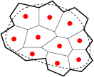
Figure 1: Schematic definition of $\tilde{\Omega}$ (bounded by thick lines) for a given domain $\Omega$ (bounded by dashed curve). Cells are represented by 2D polygons and their centers inside $\Omega$ are marked by the thick dots. Thin lines are the “internal” cell-cell interfaces which do not belong to the border of $\tilde{\Omega}.$ In reality the cells are three-dimensional and the cell-cell interfaces may not be flat.

II.2 Microscopic description of the momentum balances

We denote by ${\stackrel{{\scriptstyle\leftrightarrow}}{{\mathcal{G}}}}$ the microscopic momentum flux tensor. It is defined such that ${\stackrel{{\scriptstyle\leftrightarrow}}{{\mathcal{G}}}}\cdot d\vec{A}({\vec{r}})$ gives the flow rate of momentum across the oriented infinitesimal surface element, $d\vec{A}({\vec{r}}),$ at the position ${\vec{r}}$. We ignore completely the convective parts the linear or angular momenta which are carried by the inertia or moment of inertia, respectively. (We assume the existence of such microscopic description with microscopic but finite spatio-temporal resolutions.) Our basic starting point is the conservation laws of momentum and angular momentum,

$${\nabla\cdot{\stackrel{{\scriptstyle\leftrightarrow}}{{\mathcal{G}}}}{}^{t}=0,\qquad 0={\mbox{$\mbox{\boldmath${e}$}$}}:{\stackrel{{\scriptstyle\leftrightarrow}}{{\mathcal{G}}}}{}^{t},}$$ (1)

where ^t means to take the transposition. The second equation is nothing but the symmetry, ${\stackrel{{\scriptstyle\leftrightarrow}}{{\mathcal{G}}}}={\stackrel{{\scriptstyle\leftrightarrow}}{{\mathcal{G}}}}{}^{t},$ but we wrote above in the form similar to the final Cosserat form summarized in the final section. In either form, it means that the description by ${\stackrel{{\scriptstyle\leftrightarrow}}{{\mathcal{G}}}}$ is enough detailed that the balance of angular momentum can be expressed by the linear momentum flux alone Landau et al. (1986), that is, the torque on each surface element $d\vec{A}(\vec{r})$ is ignorable. In the setup thus defined, the quasi-static conservation of the momentum and angular momentum over the $i$-th cell reads:

$${\int_{\vec{r}\in\partial\Omega_{i}}{\stackrel{{\scriptstyle\leftrightarrow}}{{\mathcal{G}}}}\cdot d{\vec{A}}(\vec{r})=0}$$ (2)

$${\int_{\vec{r}\in\partial\Omega_{i}}\vec{r}\wedge{\stackrel{{\scriptstyle\leftrightarrow}}{{\mathcal{G}}}}\cdot d{\vec{A}}(\vec{r})=0,}$$ (3)

where integral is done over the whole boundary $\partial\Omega_{i}$ of the $i$-th cell occupying the volume $\Omega_{i},$ and $d{\vec{A}}(\vec{r})$ is the outward area element at the position $\vec{r}(\in\partial\Omega_{i}).$ We used the Gauss’ theorem of integration to derive (2) and (3) from (1).

II.3 Coarse-graining of momentum flux — “Cell”-level description of momentum balances

We rewrite the above conservation laws (2) and (3) into a reduced form to the packing of the cells. In other words we move from the space of $\vec{r}$ to the space of the indices of the cells, $\{i\}$.

Definition of inter-cellular force $F_{i,j}$ and inter-cellular torque $\vec{M}_{i,j}$ across the cell-boundary:

When the $i$-th and $j$-th cells share an interface, $\partial\Omega_{i}\cap\partial\Omega_{j}(\neq\emptyset)$, then the force and torque that the $i$-th cell applies to the $j$-th cell through this interface, which we denote by $\vec{F}_{i,j}$ and $\vec{M}_{i,j},$ respectively, are given by

$${\vec{F}_{i,j}\equiv\int_{\vec{r}\in\partial\Omega_{i}\cap\partial\Omega_{j}}{\stackrel{{\scriptstyle\leftrightarrow}}{{\mathcal{G}}}}\cdot d\vec{A}_{i\rightarrow j}(\vec{r})}$$ (4)

$${\vec{M}_{i,j}\equiv\int_{\vec{r}\in\partial\Omega_{i}\cap\partial\Omega_{j}}{[\vec{r}-(\vec{r}_{i}+\vec{a}_{i,j})]}\wedge{\stackrel{{\scriptstyle\leftrightarrow}}{{\mathcal{G}}}}\cdot d\vec{A}_{i\rightarrow j}(\vec{r}),}$$ (5)

$${\vec{a}_{i,j}=\frac{\int_{\partial\Omega_{i}\cap\partial\Omega_{j}}(\vec{r}-\vec{r}_{i})d{A}_{i\to j}(\vec{r})}{\int_{\partial\Omega_{i}\cap\partial\Omega_{j}}d{A}_{i\to j}(\vec{r})},}$$ (6)

where the surface integral is done over the interface, $\partial\Omega_{i}\cap\partial\Omega_{j},$ with $d\vec{A}_{i\rightarrow j}(\vec{r})$ being the area element at $\vec{r},$ oriented from the $i$-th cell toward the $j$-th cell.

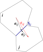
Figure 2: Definition of $\vec{a}_{i,j}$ and ${\vec{\epsilon}}_{i,j}$. The common interface $\partial\Omega_{i}\cap\partial\Omega_{j}$ is denoted by $\vec{S}_{ij}$. The center of $S_{ij}$ is written as ${\vec{r}}_{i}+\vec{a}_{i,j}$ and also as ${\vec{r}}_{j}+\vec{a}_{j,i},$ where ${\vec{r}}_{i}$ and ${\vec{r}}_{j}$ are the center positions of the cell $i$ and cell $j$, respectively.

The vector $\vec{a}_{i,j}$ is the relative position from $\vec{r}_{i}$ to the areal center of the interface, $\partial\Omega_{i}\cap\partial\Omega_{j},$ see Fig. 2. In this figure the center-to-center vector ${\vec{\epsilon}}_{i,j}$ is also introduced as

$${{\vec{\epsilon}}_{i,j}={\vec{r}}_{j}-{\vec{r}}_{i},}$$ (7)

which satisfies the geometrical relation, $\vec{a}_{i,j}-\vec{a}_{j,i}={\vec{\epsilon}}_{i,j},$ and will eventually take place of $\vec{a}_{i,j}$ and $\vec{a}_{j,i}$ in the final results. We can see that the torque $\vec{M}_{i,j}$ in (5) is measured with respect to $\vec{r}_{i}+\vec{a}_{i,j}$, i.e., the center of the interface, ${\partial\Omega_{i}\cap\partial\Omega_{j}}.$ While the apparent $\vec{r}_{i}$ in (5) and that in (6) cancel with each other, we retain them since the physical meaning of the torque $\vec{M}_{i,j}$ is clearer in this form. The integrals over each interface in (4) and (5) realize the first step of the coarse-graining of momentum by masking all the detailed informations in ${\stackrel{{\scriptstyle\leftrightarrow}}{{\mathcal{G}}}}$ except for its zeroth ($\vec{F}$) and first ($\vec{M}$) moments while keeping track of the conserved nature of the linear and angular momentum.

Reciprocity relations for $\vec{F}_{i,j}$ and $\vec{M}_{i,j}$:

The definitions (4) and (5) together with the trivial geometrical identity, $d\vec{A}_{i\rightarrow j}(\vec{r})+d\vec{A}_{j\rightarrow i}(\vec{r})=\vec{0},$ lead to the following reciprocity relations about the interface between the neighboring cell-pair, $i$ and $j$:

$$\vec{F}_{i,j}+\vec{F}_{j,i}=\vec{0},\qquad\vec{M}_{i,j}+\vec{M}_{j,i}=\vec{0}.$$ (8)

These express the conserved nature of momentum flux, or Newton’s third law, across the mesoscopic cell-cell interface.

Kirchhoff-type laws for $\vec{F}_{i,j}$ and $\vec{M}_{i,j}$ :

The conserved nature of momentum flux can be also expressed for each coarse-graining cell. The definitions (4) and (5) with the simple identity, $\partial\Omega_{i}=\cup_{j}(\partial\Omega_{i}\cap\partial\Omega_{j}),$ allows to rewrite the balance laws, (2) and (3), into the following Kirchhoff-type laws:

$$\sum_{j}^{(i)}\vec{F}_{i,j}=\vec{0},$$ (9)

$$\sum_{j}^{(i)}\left(\vec{M}_{i,j}+\vec{a}_{i,j}\wedge\vec{F}_{i,j}\right)=\vec{0},$$ (10)

where the sum $\sum_{j}^{(i)}$ runs over all the cells indexed by $j$ for which the $i$-th cell is an immediate neighbor. Notice that the flows $\vec{F}_{i,j}$ or $\vec{M}_{i,j}$ in (8) or (9) and (10) do not imply exclusively the two-body interactions between the cell pairs.

Identities for an arbitrary domain $\Omega$ :

Using each coarse-graining cell as a building block, the Kirchhoff-type law for a single cell can be extended to any closure domain, $\tilde{\Omega}$, that is :

$$\int_{\vec{r}\in\partial\tilde{\Omega}}{\stackrel{{\scriptstyle\leftrightarrow}}{{\mathcal{G}}}}\cdot d{\vec{A}}(\vec{r})=\sum_{\vec{r}_{i}\in\Omega}\left\{\sum_{j}^{(i)}\vec{F}_{i,j}\right\},$$ (11)

$$\int_{\vec{r}\in\partial\tilde{\Omega}}\vec{r}\wedge{\stackrel{{\scriptstyle\leftrightarrow}}{{\mathcal{G}}}}\cdot d{\vec{A}}(\vec{r})=\sum_{\vec{r}_{i}\in\Omega}\left\{\sum_{j}^{(i)}\left(\vec{M}_{i,j}+\vec{a}_{i,j}\wedge\vec{F}_{i,j}\right)\right\},$$ (12)

where the integrals over the cell-cell interface inside of $\tilde{\Omega}$ on the left hand side cancel among them. On the right hand side such cancellation is implied by the reciprocity properties given by (8).

III Empirical “neighbor distribution function”

The next and crucial step is to rewrite (9) and (10) for a cell $\Omega_{i}$ in the forms which are more adapted to the continuous field representation. The sums in (9) and (10) contain delicate cancellations which are closely associated to the reciprocity, (8). In order to get rid of such cancellations, the new idea, to our knowledge, is to use a local “neighbor distribution function”, $\hat{\rho}_{2FM}$.

Definition of neighbor distribution function, $\hat{\rho}_{2FM}$:

This is an empirical and simultaneous distribution function of the center distance ${\vec{\epsilon}}$, the cell-to-cell force $\vec{F}$ and cell-to-cell torque $\vec{M}$ associated to a cell at the position ${\vec{r}}$ and its immediate neighbor.

$$\hat{\rho}_{2FM}\left(\vec{\epsilon},\vec{F},\vec{M},\vec{r}\right)\equiv\sum_{i}\sum_{j}^{(i)}\delta\left({\vec{\epsilon}}-{\vec{\epsilon}}_{i,j}\right)\delta\left(\vec{F}-\vec{F}_{i,j}\right)\delta\left(\vec{M}-\vec{M}_{i,j}\right)\delta\left(\vec{r}-\vec{r}_{i}\right).$$ (14)

(The word “empirical” is used in the sense of the particular sample of statistical ensemble, and throughout this paper, we will use the “hat” symbol like $\hat{A}$ to denote those empirical quantities which are before the statistical averaging.) For the simplicity of notations, we will also use the “peripheral” or partially integrated neighbor distribution functions, such as $\hat{\rho}_{2F}(\vec{\epsilon},\vec{F},\vec{r})\equiv\sum_{i}\sum_{j}^{(i)}\delta(\vec{F}-\vec{F}_{i,j})$$\delta\left(\vec{r}_{i}-\vec{r}\right)$$\delta\left(\vec{r}_{j}-\vec{r}_{i}-\vec{\epsilon}\right),$ and $\hat{\rho}_{2M}(\vec{\epsilon},\vec{M},\vec{r})\equiv\sum_{i}\sum_{j}^{(i)}$$\delta(\vec{M}-\vec{M}_{i,j})$$\delta\left(\vec{r}_{i}-\vec{r}\right)$
$\delta\left(\vec{r}_{j}-\vec{r}_{i}-\vec{\epsilon}\right).$ Also we will use the purely geometrical neighbor distribution, $\hat{\rho}_{2}\left(\vec{\epsilon},\vec{r}\right)\equiv\sum_{i}\sum_{j}^{(i)}\delta\left(\vec{r}_{i}-\vec{r}\right)\delta\left(\vec{r}_{j}-\vec{r}_{i}-\vec{\epsilon}\right).$ The further integration of $\hat{\rho}_{2}({\vec{\epsilon}},{\vec{r}})$ over ${\vec{\epsilon}}$ yields $\int\hat{\rho}_{2}\left(\vec{\epsilon},\vec{r}\right)d^{3}{\vec{\epsilon}}=(\sum_{j}^{(i)}1)\sum_{i}\delta\left(\vec{r}_{i}-\vec{r}\right),$ where multiplicative factor, $\sum_{j}^{(i)}1,$ is the number of neighbors of the $i$-th cell, and the remainder defines the empirical single-cell density function, $\hat{\rho}_{1}$ :

$$\hat{\rho}_{1}\left(\vec{r}\right)\equiv\sum_{i}\delta\left(\vec{r}_{i}-\vec{r}\right).$$ (15)

The neighbor density distribution, $\hat{\rho}_{2FM},$ contains the detailed informations about ${\vec{\epsilon}}_{i,j}=\vec{r}_{j}-\vec{r}_{i}$, $\vec{F}_{i,j}$ and $\vec{M}_{i,j}.$ This function should be well distinguished from any weighting function that is introduced for the purpose of smoothing. The right hand sides of (11) can be rewritten as moment integrals of $\hat{\rho}_{2FM}$. Leaving the derivation to Appendix A, the result reads

$$\int_{\vec{r}\in\partial\tilde{\Omega}}{\stackrel{{\scriptstyle\leftrightarrow}}{{\mathcal{G}}}}\cdot d{\vec{A}}(\vec{r})=\int_{\vec{r}\in\Omega}{\left[{{\int\!\!\!\int\!}\vec{F}\,\hat{\rho}_{2F}(\vec{\epsilon},\vec{F},\vec{r})\,d^{3}\vec{F}\,d^{3}\vec{\epsilon}}\right]}\,d^{3}\vec{r},$$ (16)

$$\int_{\vec{r}\in\partial\tilde{\Omega}}\vec{r}\wedge{\stackrel{{\scriptstyle\leftrightarrow}}{{\mathcal{G}}}}\cdot d{\vec{A}}(\vec{r})$$ (17)

$$=\int_{\vec{r}\in\Omega}\!\!{\left[{{\int\!\!\!\int\!\!\!\int\!}(\vec{M}\,+\frac{1}{2}\vec{\epsilon}\wedge\vec{F})\hat{\rho}_{2FM}(\vec{\epsilon},\vec{F},\vec{M},\vec{r})\,d^{3}\vec{\epsilon}\,d^{3}\vec{M}\,d^{3}\vec{F}}\right]}d^{3}\vec{r}.$$ (18)

Redundancy of $\hat{\rho}_{2FM}(\vec{\epsilon},\vec{F},\vec{M},\vec{r})$:

By looking at the pair of neighboring cells at $\vec{r}$ and at $\vec{r}+{\vec{\epsilon}}$ in two ways, the reciprocity relations (8) are expressed as a redundancy property of the neighbor distribution function :

$${\hat{\rho}_{2FM}\left(\vec{\epsilon},\vec{F},\vec{M},\vec{r}\right)=\hat{\rho}_{2FM}\left(-\vec{\epsilon},-\vec{F},-\vec{M},\vec{r}+\vec{\epsilon}\right).}$$ (20)

The derivation is given in Appendix B, but the contents may be intuitively understandable. The associated peripheral distributions inherit the similar relations :

$$\hat{\rho}_{2F}\left(\vec{\epsilon},\vec{F},\vec{r}\right)=\hat{\rho}_{2F}\left(-\vec{\epsilon},-\vec{F},\vec{r}+\vec{\epsilon}\right),$$ (21)

$$\hat{\rho}_{2M}\left(\vec{\epsilon},\vec{M},\vec{r}\right)=\hat{\rho}_{2M}\left(-\vec{\epsilon},-\vec{M},\vec{r}+\vec{\epsilon}\right).$$ (22)

The redundancy relation implies the following identities, whose derivations are given in Appendix C:

$${\int\!\!\!\int\!}\vec{F}\hat{\rho}_{2F}\left(\vec{\epsilon},\vec{F},\vec{r}\right)\,d^{3}\vec{F}\,d^{3}\vec{\epsilon}$$ (23)

$$={\frac{1}{2}}{\int\!\!\!\int\!}\vec{F}\,{\left[{\hat{\rho}_{2F}\left(\vec{\epsilon},\vec{F},\vec{r}\right)-\hat{\rho}_{2F}\left(\vec{\epsilon},\vec{F},\vec{r}-\vec{\epsilon}\right)}\right]}\,d^{3}\vec{F}\,d^{3}\vec{\epsilon}$$ (24)

$${\int\!\!\!\int\!}\vec{\epsilon}\otimes\vec{\epsilon}\otimes\vec{F}\hat{\rho}_{2F}\left(\vec{\epsilon},\vec{F},\vec{r}\right)\,d^{3}\vec{F}\,d^{3}\vec{\epsilon}$$ (26)

$$+{\int\!\!\!\int\!}\vec{\epsilon}\otimes\vec{\epsilon}\otimes\vec{F}\hat{\rho}_{2F}\left(\vec{\epsilon},\vec{F},\vec{r}-\vec{\epsilon}\right)\,d^{3}\vec{F}\,d^{3}\vec{\epsilon}=0$$ (27)

These identities will be used below (§ IV) to get rid of the delicate cancellations in the Kirchhoff-Type laws, (9) and (10).

IV Macroscopic fluxes of momentum and angular momentum

IV.1 Statistically averaged neighbor distributions

As long as the size of the coarse-graining cells is properly chosen (see §§ II.1), the statistical properties of the neighbor distribution function $\hat{\rho}_{2FM}$ should be mostly homogeneous over the spatial domain $\Omega$ whose diameter is well above the former size but, at the same time, well below the characteristic spatial scale at which the macroscopic state varies. When a function including $\hat{\rho}_{2FM}$ as a factor is integrated over the whole ${\vec{\epsilon}}$-, $\vec{F}$- and $\vec{M}$- domains but limited over the ${\vec{r}}$-domain $\Omega$, we can replace $\hat{\rho}_{2FM}$ by its statistical average as a good approximation thanks to the law of large number. We will denote by ${\rho}_{2FM}$ without “$\,\,\hat{\mbox{}}\,\,$” the statistical average of $\hat{\rho}_{2FM}.$ We will use this averaged distribution function with the understanding that all the macroscopic properties can be calculated through the integral over the above mentioned semi-macroscopic domain $\Omega$ (or its closure $\tilde{\Omega}$), see for example (16) and (17). The statistically averaged version of the peripheral distribution functions, $\rho_{2F}({\vec{\epsilon}},\vec{F},\vec{r}),$ ${\rho}_{2M}({\vec{\epsilon}},\vec{M},\vec{r}),$ $\rho_{2}({\vec{\epsilon}},\vec{r})$ and $\rho_{1}(\vec{r}),$ are also introduced. Under the same premise, the empirical number of cell neighbors, $\hat{Z}$, is replaced by its statistical average, $Z(\vec{r}),$ which is defined through

$${Z(\vec{r})\rho_{1}(\vec{r})\equiv\int{\rho_{2}\left(\vec{\epsilon},\vec{r}\right)}d^{3}\vec{\epsilon}.}$$ (28)

The statistically averaged neighbor distribution function, ${\rho}_{2FM},$ and its peripheral distributions should be slowly varying functions in space, ${\vec{r}}$. They, therefore, allow the gradient expansion in ${\vec{\epsilon}},$ that is, the spatial derivative operation with respect to ${\vec{r}}$, which we denote by $\nabla$, satisfies the property, $\|{\vec{\epsilon}}\cdot\nabla\|\ll 1,$ where $\|{\vec{\epsilon}}\|$ is the typical center-to-center distance of neighboring cell pairs. We will use this expansion below.

IV.2 Expression for the macroscopic fluxes

In the integral conservation relations, (16) and (17), we apply the redundancy relations (21) and (22), in the way shown in (23) or its homologous form with $\vec{F}$ and $\vec{M}$ being exchanged. Then we replace the empirical distributions by the statistical averaged ones to apply the gradient expansion mentioned above. The higher order terms in the expansion is much smaller than the first order, which we can verify using the identity (26). Leaving the details of derivation in Appendices D and E, the results read as follows.

For the macroscopic momentum flux ${\stackrel{{\scriptstyle\leftrightarrow}}{{G}}},$ it satisfies the local momentum conservation,

$$\nabla\cdot{\stackrel{{\scriptstyle\leftrightarrow}}{{G}}}=\vec{0}.$$ (29)

under the definition:

$${{\stackrel{{\scriptstyle\leftrightarrow}}{{G}}}({\vec{r}})\equiv\frac{Z({\vec{r}})\rho_{1}({\vec{r}})}{2}\langle{\vec{\epsilon}}\otimes\vec{F}\rangle_{2}({\vec{r}}),}$$ (30)

where $\langle\,\mathcal{\psi}\rangle_{2}({\vec{r}})$ stands for the average of $\mathcal{\psi}$ with the statistically averaged neighbor distribution function ${\rho}_{2FM}$,

$$\langle\mathcal{\psi}\rangle_{2}({\vec{r}}) \equiv \frac{{\int\!\!\!\int\!\!\!\int\!}\mathcal{\psi}\,\,{\rho}_{2FM}\left(\vec{\epsilon},\vec{F},\vec{M},\vec{r}\right)\,d^{3}\vec{M}\,d^{3}\vec{F}\,d^{3}\vec{\epsilon}}{{\int\!\!\!\int\!\!\!\int\!}{\rho}_{2FM}\left(\vec{\epsilon},\vec{F},\vec{r}\right)\,d^{3}\vec{M}\,d^{3}\vec{F}\,d^{3}\vec{\epsilon}}$$ (31)

$$= \frac{{\int\!\!\!\int\!\!\!\int\!}\mathcal{\psi}\,\,{\rho}_{2FM}\left(\vec{\epsilon},\vec{F},\vec{M},\vec{r}\right)\,d^{3}\vec{M}\,d^{3}\vec{F}\,d^{3}\vec{\epsilon}}{Z(\vec{r})\rho_{1}(\vec{r})}.$$ (32)

For the macroscopic angular momentum flux ${\stackrel{{\scriptstyle\leftrightarrow}}{{{C}}}},$ it satisfies

$$\nabla\cdot{\stackrel{{\scriptstyle\leftrightarrow}}{{{C}}}}=-{\mbox{$\mbox{\boldmath${e}$}$}}:{\stackrel{{\scriptstyle\leftrightarrow}}{{G}}},$$ (33)

under the definition:

$${{\stackrel{{\scriptstyle\leftrightarrow}}{{{C}}}}({\vec{r}})\equiv{\frac{Z({\vec{r}})\rho_{1}({\vec{r}})}{2}\langle{\vec{\epsilon}}\otimes\vec{M}\rangle_{2}({\vec{r}})}.}$$ (34)

While the Eqs. (30) and (34) used the factorization of $Z({\vec{r}})$ and $\rho_{1}({\vec{r}})$ to conform with the original IK formula, what are to calculate is the moments of $\rho_{2FM}({\vec{\epsilon}},\vec{F},\vec{M},{\vec{r}})$, such as ${\int\!\!\!\int\!}\vec{\epsilon}\otimes\vec{F}\,\rho_{2F}\left(\vec{\epsilon},\vec{F},\vec{r}\right)\,d^{3}\vec{F}\,d^{3}\vec{\epsilon}$ in Eq.(51). Under a quasi-uniformly packed compartments, $\{\Omega_{i}\}$, the factors $Z({\vec{r}})$ and $\rho_{1}({\vec{r}})$ are mostly uniform and constant. The relevant macro-variables are rather the flows of mass, momentum and angular momentum and some order parameters such as the mean polarity of the cellular units.

V Conclusion and discussion

We recognized that, in the media undergoing the quasi-steady processes, (i) the Cosserat-type equations provide with the general principle of macroscopic characterization of the linear and angular momenta, (29) and (33), and that (ii) the Irving-Kirkwood-type or virial-type formulas provide with the general principle of transformation of these momenta from mesoscopic to macroscopic level, (30) and (34), where $\vec{F}$ and $\vec{M}$ are, respectively, the flow rate of linear and angular momenta that pass through the hypothetical interface between a pair of coarse-graining cells with ${\vec{\epsilon}}$ being their center-to-center distance. The average $\langle\cdot\rangle_{2}(\vec{r})$ defined by (31) essentially samples over many pairs of coarse-graining cells around the given position $\vec{r}$ with $Z({\vec{r}})\rho_{1}({\vec{r}})/2$ being the spatial density of such pairs. For those complex and non-equilibrium systems whose micro-variables and dynamics are unknown or too complicated, it is a matter of choice whether we take a completely phenomenological approach to correlate directly the macro flux variables to the macro state variables (e.g. Kruse et al. (2004, 2005)), or, otherwise, we take an indirect approach that takes advantage of the statistical mechanics, which is our choice.

Our results are distinguished from the original Irving-Kirkwood (IK) formulas: We relate the macroscopic fluxes to those flows of momentum and angular momentum which are attributed to each mesoscopic cells, or volume elements, over which we carry out our first step of coarse-graining. Unlike the conventional scheme the variables such as distance vectors, forces or torques among the microscopic model elements (i.e., the molecules or grains) do not appear there. Our IK-type formulas consist of, instead of the inter-particle force or torque, the linear and angular momentum flows across the interface separating the neighboring coarse-graining cells and, instead of the inter-particle distance, there appear the distance between the centers of these cells. Although our theory is also a “bottom-up” construction, we coarse-grain the mesoscopic momentum flux instead of any microscopic dynamical model. The coarse graining without micro-variables or dynamics is possible because we deal with just as many components for the two conserved vector fields to derive the two vectorial conservation laws.

Once the correct IK-type formulas for the fluxes are given, they naturally satisfy the Cosserat-type equations whatever is the microscopic ingredients. This logic is consistent with the “microscopic” Cosserat equations in Eringen and Kafadar (1976) (the Eqs. (1.4.12) and (1.4.13) in Part I), where the authors obtained as an equivalent form of the balance equations of momentum and angular momentum without coarse-graining but with a continuum field theory of polar fluid containing the microscopic angular momentum density (“spin”).

Our work thus reveals the universality of Cosserat type equations and Irving-Kirkwood type formulas through an abstract procedure of the coarse-graining. Although being much in narrower sense than the Newton’s laws or the laws of thermodynamics as general principles, we assert that the Cosserat type equations and Irving-Kirkwood type formulas are still the principles that apply to a wide class of phenomena than were ever discussed. In these principle, the size of the coarse-graining cell could be different from that of the constituent individual elements of the system when, for example, those elements form local clusters.

An important outcome of our finding is its applicability to the systems of densely packed active elements such as amoeba cells. In fact it was such system that first motivated us to develop the present framework. As mentioned in §I, the interaction and dynamics of such system is usually very complicated. Even under such circumstances our theory can still tell that (i) the Cosserat-type equations in terms of the fluxes, ${\stackrel{{\scriptstyle\leftrightarrow}}{{G}}}$ and ${\stackrel{{\scriptstyle\leftrightarrow}}{{C}}}$, are the canonical representation of the flux balance at the macroscopic level and that (ii) it is the flows $\vec{F}$ and $\vec{M}$ associated to the coarse-graining cell interfaces that should be found in order to calculate ${\stackrel{{\scriptstyle\leftrightarrow}}{{G}}}$ and ${\stackrel{{\scriptstyle\leftrightarrow}}{{C}}}.$ Our framework thus provides a new toolbox to those domains of research which have not been exploited by the kinetic theories of gases and granular matters or the theory of continuum with inclusions.

(a)

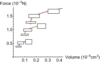
(b)

Figure 3: (a) The experimental stall forces generated by an aggregate of Dictyostelium Discoideum when its directed collective movement in a tube is impeded either by a pressure gradient (blue dots, “Non centrifugal”) or by a centrifugal force (red, “Centrifugal”). The data are extracted from Inoue et al. (Inouye and Takeuchi (1980) Fig. 5 and Inouye (1984) Fig. 5). (b) Model prediction of the stall force using the present framework for the macroscopic momentum and angular momentum fluxes. The results are reproduced from Fruleux (2014) Fig. 9.14. The model is two-dimensional and the rectangular symbols represent the shape and dimensions of the aggregates. Those aggregates with the same length along the tube axis are grouped by the continuous curves.

In order to apply to specific setup, we need to supplement with proper boundary conditions adapted to the characteristic of the system. Unlike the conventional hydrodynamics of viscous fluids, the no-slip boundary condition is not a priori assured and we should carefully choose the appropriate ones case by case.

Although the case studies are not our purpose in the present paper, we briefly introduce below a comparison between the theory using the present framework Fruleux (2014) and the experiments done about the force generation by the aggregate of Dictyostelium Discoideum Gilbert and Epel (2009). The experiments have measured the stall force of the aggregate when its collective movement is impeded by an adjustable external force. The stall force was found to depend approximatively linearly on the volume of the aggregates Inouye and Takeuchi (1980); Inouye (1984), see Fig. 3(a). This result was intriguing because, if the locomotive cells were simply packed with an aligned polarity, only those cells at the surface of the aggregate could contribute to the locomotive force, implying the proportionality of the stall force to the contact area with the substrate surface. In the theory Fruleux (2014) the effect of the local deviations of the polarity of cells in the presence of the substrate are taken into account. The resultant linear and angular momentum flows among the cells are modeled for $\vec{F}_{i,j}$ and $\vec{M}_{i,j}$ through the (pair) neighbor distribution function, $\rho_{2FM},$ with a due consideration of the boundary conditions. In order to evaluate $\rho_{2FM}$ the theory Fruleux (2014) not only uses the known behavioral facts about the ‘crawling’ of individual cells in a dense environment but also introduces the three-neighbor distribution function. Since the microscopic dynamics for the “cells” is not available, the three-neighbor distribution function is not related through BBGKY-like hierarchy to $\rho_{2FM}.$ Instead, an extensive use have been made of the redundancy properties of the former function. The neighbor distribution functions in our new approach, $\rho_{2FM}$, plays the central role bridging between the mesoscopic flow rates, $\vec{F}_{i,j}$ and $\vec{M}_{i,j}$, and the macroscopic rheological variables. The analysis of the model predicted the stall force that increases with the volume of the aggregates, see Fig. 3(b). In this model those cells with distorted polarity constitute the boundary layers whose thickness depends on the stall force due to the non-linearity of the system. As a result the stall force should also depends on the aspect ratio of the aggregate Fruleux (2014). The theory is free of adjustable parameters, and the quantitative discrepancy about a factor $\sim 5$ could be due to the basic parameters taken from different literatures.

While the main advantage of the present framework is its applicability to the materials consisting of complex mesoscopic elements, our formalism may also shed new light on the existing theories on the gas kinetics and polar fluid dynamics (see, for example, Weinhart et al. (2012) and the references cited therein): Many efficient methods of coarse-graining which have been developed so far, such as through the Chapman-Enskog theory, the moment integrals Eringen and Kafadar (1976); Dahler and Theodosopulu (2007); Irving and Kirkwood (1950), or integral over space-time with weighting functions Babic (1997) or test function Eringen and Kafadar (1976), have sometimes put more priority on some physical or practical aspects other than the conservation of linear- and angular-momenta. For example, if we use the volume or spatio-temporal integral of the microscopic forces over a coarse-graining (space-time) volume with some weighting function, the conserved nature of the microscopic momentum may not be automatically inherited by the resulting coarse-grained system. That is, the macroscopic fluxes might obey the equations which are not exactly of the Cosserat-type. In particular, the source of divergence of angular momentum flux ($-{\mbox{$\mbox{\boldmath${e}$}$}}:{\stackrel{{\scriptstyle\leftrightarrow}}{{G}}}$ for the Cosserat-type) would be different from the antisymmetric part of the momentum flux (${\stackrel{{\scriptstyle\leftrightarrow}}{{G}}}$) which appears in the conservation of the linear momentum ($\nabla\cdot{\stackrel{{\scriptstyle\leftrightarrow}}{{G}}}=0$). For example, in Dahler and Theodosopulu (2007), the structure of the Cosserat equations is lost because the moment integrals used there do not necessarily assure the flux conservation. Logically, such theory can also be correct about the momentum conservation if the modifications from the IK-type fluxes are exactly compensated by the modifications from the Cosserat-type equations. Our purpose, however, is to provide with a framework that observes explicitly the momentum balance at the mesoscopic scale so that we can focus on the modeling of the mesoscopic flows. To our knowledge there is only a few paper that used the coarse-graining along this line for non-polar fluids Todd et al. (1995). There the authors used the surface integral instead of the volume integral of the momentum flux although they focused rather on the numerical improvement than the conservation issue.

Appendix A Derivation of (16) and (17)

First we show

$$\sum_{\vec{r}_{i}\in\Omega}\left\{\sum_{j}^{(i)}\vec{F}_{i,j}\right\}=\int_{\vec{r}\in\Omega}{\int\!\!\!\int\!}\vec{F}\,\hat{\rho}_{2F}(\vec{\epsilon},\vec{F},\vec{r})\,d^{3}\vec{F}\,d^{3}\vec{\epsilon}\,d^{3}\vec{r}$$ (35)

and

$$\sum_{\vec{r}_{i}\in\Omega}\left\{\sum_{j}^{(i)}\vec{M}_{i,j}\right\}=\int_{\vec{r}\in\Omega}{\int\!\!\!\int\!}\vec{M}\,\hat{\rho}_{2M}(\vec{\epsilon},\vec{M},\vec{r})\,d^{3}\vec{M}\,d^{3}\vec{\epsilon}\,d^{3}\vec{r}$$ (36)

for arbitrary $\Omega$. Eq. (35) holds because

$$\sum_{\vec{r}_{i}\in\Omega}\left\{\sum_{j}^{(i)}\vec{F}_{i,j}\right\} = \int_{\vec{r}\in\Omega}\int\sum_{i}\sum_{j}\vec{F}_{i,j}\delta\left(\vec{r}_{j}-\vec{r}\right)\delta\left(\vec{r}_{j}-\vec{r}_{i}-\vec{\epsilon}\right)\,d^{3}\vec{\epsilon}\,d^{3}\vec{r}$$ (37)

$$= \int_{\vec{r}\in\Omega}{\int\!\!\!\int\!}\sum_{i}\sum_{j}\vec{F}\delta\left(\vec{F}-\vec{F}_{i,j}\right)\delta\left(\vec{r}_{j}-\vec{r}\right)\delta\left(\vec{r}_{j}-\vec{r}_{i}-\vec{\epsilon}\right)\,d^{3}\vec{F}\,d^{3}\vec{\epsilon}\,d^{3}\vec{r}$$

$$= \int_{\vec{r}\in\Omega}{\int\!\!\!\int\!}\vec{F}\,\hat{\rho}_{2F}(\vec{\epsilon},\vec{F},\vec{r})\,d^{3}\vec{F}\,d^{3}\vec{\epsilon}\,d^{3}\vec{r}$$ (38)

The equality for the torque (36) can be shown similarly. Next, combining the above results with (11) we have the identities,

$$\int_{\vec{r}\in\partial\tilde{\Omega}}\vec{r}\wedge{\stackrel{{\scriptstyle\leftrightarrow}}{{\mathcal{G}}}}\cdot d{\vec{A}}(\vec{r})=-\int_{\vec{r}\in\Omega}{\int\!\!\!\int\!}\vec{M}\,\hat{\rho}_{2M}(\vec{\epsilon},\vec{M},\vec{r})\,d^{3}\vec{M}\,d^{3}\vec{\epsilon}\,d^{3}\vec{r}-\sum_{\vec{r}_{i}\in\Omega}\left\{\sum_{j}^{(i)}\vec{a}_{i,j}\wedge\vec{F}_{i,j}\right\}$$ (39)

On the r.h.s., $\sum_{\vec{r}_{i}\in\Omega}\sum_{j}^{(i)}\left(\vec{a}_{i,j}\wedge\vec{F}_{i,j}\right)$ can also be represented as a moment integral: we first notice that this sum is equal to $\frac{1}{2}\sum_{\vec{r}_{i}\in\Omega}\sum_{j}^{(i)}\left(\vec{a}_{i,j}-\vec{a}_{{j,i}}\right)\wedge\vec{F}_{i,j}$. Then, by the geometrical identity $\vec{a}_{i,j}-\vec{a}_{i,j}={\vec{\epsilon}}_{i,j}$, we have $\sum_{\vec{r}_{i}\in\Omega}\sum_{j}^{(i)}\left(\vec{a}_{i,j}\wedge\vec{F}_{i,j}\right)=\frac{1}{2}\sum_{\vec{r}_{i}\in\Omega}\sum_{j}{\vec{\epsilon}}_{i,j}\wedge\vec{F}_{i,j},$ which is written as $\frac{1}{2}\int_{\vec{r}\in\Omega}{\left({{\int\!\!\!\int\!}\vec{\epsilon}\wedge\vec{F}\,\,\rho_{2F}\left(\vec{\epsilon},\vec{M},\vec{r}\right)\,d^{3}\vec{\epsilon}\,d^{3}\vec{M}}\right)}d^{3}\vec{r}.$ Therefore, (39) reads (17). (End of derivation)

Appendix B Derivation of (20)

In the definition of $\hat{\rho}_{2FM}$ (see (14))

$$\hat{\rho}_{2FM}\left(\vec{\epsilon},\vec{F},\vec{M},\vec{r}\right)\equiv\sum_{i}\sum_{j}^{(i)}\delta\left(\vec{r}_{j}-\vec{r}_{i}-\vec{\epsilon}\right)\delta\left(\vec{F}-\vec{F}_{i,j}\right)\delta\left(\vec{M}-\vec{M}_{i,j}\right)\delta\left(\vec{r}-\vec{r}_{i}\right)$$

we change the argument as follows;

$$\hat{\rho}_{2FM}\left(-\vec{\epsilon},-\vec{F},-\vec{M},\vec{r}+\vec{\epsilon}\right) = \sum_{i}\sum_{j}^{(i)}\delta\left(\vec{r}_{j}-\vec{r}_{i}-\vec{\epsilon}\right)\delta\left(\vec{F}+\vec{F}_{i,j}\right)\delta\left(\vec{M}+\vec{M}_{i,j}\right)\delta\left(\vec{r}+\vec{\epsilon}-\vec{r}_{i}\right)$$ (40)

$$= \sum_{i}\sum_{j}^{(i)}\delta\left(\vec{r}_{j}-\vec{r}_{i}-\vec{\epsilon}\right)\delta\left(\vec{F}+\vec{F}_{i,j}\right)\delta\left(\vec{M}+\vec{M}_{i,j}\right)\delta\left(\vec{r}-\vec{r}_{j}\right).$$ (41)

Using the fact that the counting of all the immediate neighbors through the sum, $\sum_{i}\sum_{j}^{(i)},$ is equivalent to that through $\sum_{j}\sum_{i}^{(j)}$, the last line becomes

$$\hat{\rho}_{2FM}\left(-\vec{\epsilon},-\vec{F},-\vec{M},\vec{r}+\vec{\epsilon}\right)=\sum_{j}\sum_{i}^{(j)}\delta\left(\vec{r}_{j}-\vec{r}_{i}-\vec{\epsilon}\right)\delta\left(\vec{F}+\vec{F}_{i,j}\right)\delta\left(\vec{M}+\vec{M}_{i,j}\right)\delta\left(\vec{r}-\vec{r}_{j}\right)$$

Finally, the reciprocity relations, $\vec{F}_{i,j}=-\vec{F}_{j,i}$ and $\vec{M}_{i,j}=-\vec{M}_{j,i}$ gives

$$\hat{\rho}_{2FM}\left(-\vec{\epsilon},-\vec{F},-\vec{M},\vec{r}+\vec{\epsilon}\right) = \sum_{j}\sum_{i}^{(j)}\delta\left(\vec{r}_{j}-\vec{r}_{i}-\vec{\epsilon}\right)\delta\left(\vec{F}-\vec{F}_{j,i}\right)\delta\left(\vec{M}-\vec{M}_{j,i}\right)\delta\left(\vec{r}-\vec{r}_{j}\right)$$ (42)

$$= \hat{\rho}_{2FM}\left(\vec{\epsilon},\vec{F},\vec{M},\vec{r}\right).$$ (43)

We thus arrived at the basic redundancy relationship (20) claimed above. The associated relations for the peripheral distributions can be obtained by integrating over either $\vec{M}$ or $\vec{F}$. (End of derivation.)

Appendix C Derivation of (23) and (26)

For (23),

$${\int\!\!\!\int\!}\vec{F}\hat{\rho}_{2F}\left(\vec{\epsilon},\vec{F},\vec{r}\right)\,d^{3}\vec{F}\,d^{3}\vec{\epsilon} ={\frac{1}{2}}{\left[{{\int\!\!\!\int\!}\vec{F}\hat{\rho}_{2F}\left(\vec{\epsilon},\vec{F},\vec{r}\right)\,d^{3}\vec{F}\,d^{3}\vec{\epsilon}+{\int\!\!\!\int\!}\vec{F}\hat{\rho}_{2F}\left(-\vec{\epsilon},-\vec{F},\vec{r}+\vec{\epsilon}\right)\,d^{3}\vec{F}\,d^{3}\vec{\epsilon}}\right]}$$ (46)

$$={\frac{1}{2}}{\left[{{\int\!\!\!\int\!}\vec{F}\hat{\rho}_{2F}\left(\vec{\epsilon},\vec{F},\vec{r}\right)\,d^{3}\vec{F}\,d^{3}\vec{\epsilon}+{\int\!\!\!\int\!}(-\vec{F})\hat{\rho}_{2F}\left(\vec{\epsilon},\vec{F},\vec{r}+(-\vec{\epsilon})\right)\,d^{3}\vec{F}\,d^{3}\vec{\epsilon}}\right]}$$

$$={\frac{1}{2}}{\int\!\!\!\int\!}\vec{F}\,{\left[{\hat{\rho}_{2F}\left(\vec{\epsilon},\vec{F},\vec{r}\right)-\hat{\rho}_{2F}\left(\vec{\epsilon},\vec{F},\vec{r}-\vec{\epsilon}\right)}\right]}\,d^{3}\vec{F}\,d^{3}\vec{\epsilon}.$$

For (26)

$${\int\!\!\!\int\!}\vec{\epsilon}\otimes\vec{\epsilon}\otimes\vec{F}\hat{\rho}_{2F}\left(\vec{\epsilon},\vec{F},\vec{r}\right)\,d^{3}\vec{F}\,d^{3}\vec{\epsilon} ={\int\!\!\!\int\!}\vec{\epsilon}\otimes\vec{\epsilon}\otimes\vec{F}\hat{\rho}_{2F}\left(-\vec{\epsilon},-\vec{F},\vec{r}+\vec{\epsilon}\right)\,d^{3}\vec{F}\,d^{3}\vec{\epsilon}$$ (48)

$$=-{\int\!\!\!\int\!}\vec{\epsilon}\otimes\vec{\epsilon}\otimes\vec{F}\hat{\rho}_{2F}\left(\vec{\epsilon},\vec{F},\vec{r}-\vec{\epsilon}\right)\,d^{3}\vec{F}\,d^{3}\vec{\epsilon}.$$

By adding the l.h.s. and the 2nd line on the r.h.s., we have (26). (End of derivation)

Appendix D Derivation of (29) and (30)

We look at (16) and rewrite its right hand side. Because $\mathcal{\psi}$ will not contain $\vec{M}$ in this issue, we will use $\rho_{2F}$ to simplify the notation. According to (23) or, more precisely, to its statistically averaged version,

$${\int\!\!\!\int\!}\vec{F}{\rho}_{2F}\left(\vec{\epsilon},\vec{F},\vec{r}\right)\,d^{3}\vec{F}\,d^{3}\vec{\epsilon}={\frac{1}{2}}{\int\!\!\!\int\!}\vec{F}\,{\left[{{\rho}_{2F}\left(\vec{\epsilon},\vec{F},\vec{r}\right)-{\rho}_{2F}\left(\vec{\epsilon},\vec{F},\vec{r}-\vec{\epsilon}\right)}\right]}\,d^{3}\vec{F}\,d^{3}\vec{\epsilon}.$$ (49)

The integral on the r.h.s. can be expanded using its slowly varying nature about ${\vec{r}}$:

(r.h.s. of (49)) $$= \frac{1}{2}\nabla\cdot\left\{{\int\!\!\!\int\!}\vec{\epsilon}\otimes\vec{F}\,\rho_{2F}\left(\vec{\epsilon},\vec{F},\vec{r}\right)\,d^{3}\vec{F}\,d^{3}\vec{\epsilon}\right\}$$ (51)

$$+\frac{1}{2}\nabla\nabla:\left\{{\int\!\!\!\int\!}{\vec{\epsilon}}\otimes\vec{\epsilon}\otimes\vec{F}\,\rho_{2F}\left(\vec{\epsilon},\vec{F},\vec{r}\right)\,d^{3}\vec{F}\,d^{3}\vec{\epsilon}\right\}+\mathcal{O}\left(\|{\vec{\epsilon}}\cdot\nabla\,\|^{3}\right).$$

Now the second term on the r.h.s., which is at most $\mathcal{O}\left(\|{\vec{\epsilon}}\cdot\nabla\,\|^{2}\right)$, is in fact only $\mathcal{O}\left(\|{\vec{\epsilon}}\cdot\nabla\,\|^{3}\right)$ because the ${\vec{\epsilon}}\cdot\nabla$ expansion of (26) shows that

$$2{\int\!\!\!\int\!}\vec{\epsilon}\otimes\vec{\epsilon}\otimes\vec{F}\hat{\rho}_{2F}\left(\vec{\epsilon},\vec{F},\vec{r}\right)\,d^{3}\vec{F}\,d^{3}\vec{\epsilon}\,-\,\nabla\cdot{\int\!\!\!\int\!}{\vec{\epsilon}}\otimes\vec{\epsilon}\otimes\vec{\epsilon}\otimes\vec{F}\hat{\rho}_{2F}\left(\vec{\epsilon},\vec{F},\vec{r}\right)\,d^{3}\vec{F}\,d^{3}\vec{\epsilon}\,\simeq\,0,$$ (52)

therefore,

$$\nabla\nabla:{\left[{{\int\!\!\!\int\!}{\vec{\epsilon}}\otimes\vec{\epsilon}\otimes\vec{F}\,\rho_{2F}\left(\vec{\epsilon},\vec{F},\vec{r}\right)\,d^{3}\vec{F}\,d^{3}\vec{\epsilon}}\right]} \simeq \nabla\nabla:{\left[{{\frac{1}{2}}\nabla\cdot\left\{{\int\!\!\!\int\!}{\vec{\epsilon}}\otimes{\vec{\epsilon}}\otimes\vec{\epsilon}\otimes\vec{F}\,\rho_{2F}\left(\vec{\epsilon},\vec{F},\vec{r}\right)\,d^{3}\vec{F}\,d^{3}\vec{\epsilon}\right\}}\right]}$$ (53)

$$= \mathcal{O}\left(\|{\vec{\epsilon}}\cdot\nabla\,\|^{3}\right).$$ (54)

Therefore, the first term on the r.h.s. of (51) is a good approximation with an error of only $\mathcal{O}\left(\|{\vec{\epsilon}}\cdot\nabla\,\|^{3}\right).$ Now rewriting (51) using the notation of $\langle{\vec{\epsilon}}\otimes\vec{F}\rangle_{2}$ and the definition (30), the equation (49) becomes

$${\int\!\!\!\int\!}\vec{F}{\rho}_{2F}\left(\vec{\epsilon},\vec{F},\vec{r}\right)\,d^{3}\vec{F}\,d^{3}\vec{\epsilon}=\nabla\cdot{\stackrel{{\scriptstyle\leftrightarrow}}{{G}}}+\mathcal{O}\left(\|{\vec{\epsilon}}\cdot\nabla\,\|^{3}\right).$$

The (16) takes the form: $\int_{\vec{r}\in\partial\tilde{\Omega}}{\stackrel{{\scriptstyle\leftrightarrow}}{{\mathcal{G}}}}\cdot d{\vec{A}}(\vec{r})=\int_{\vec{r}\in\Omega}\nabla\cdot{\stackrel{{\scriptstyle\leftrightarrow}}{{G}}}\,d^{3}\vec{r}.$ for arbitrary $\Omega$ up to the errors of $\mathcal{O}\left(\|{\vec{\epsilon}}\cdot\nabla\,\|^{3}\right)$. This justifies to identify ${\stackrel{{\scriptstyle\leftrightarrow}}{{G}}}$ as the macroscopic momentum flux. In terms of the suffix, it is rather the transpose, ${\stackrel{{\scriptstyle\leftrightarrow}}{{G}}}^{t},$ that corresponds to ${\stackrel{{\scriptstyle\leftrightarrow}}{{\mathcal{G}}}}$ due to our choice of representation of the latter. Finally (3) leads to (29). (End of derivation)

Appendix E Derivation of (33) and (34)

By a completely parallel argument as the derivation of the previous theorem, a part of the integral on the r.h.s. of (17) can be rewritten as:

$$\int_{\vec{r}\in\Omega}{\int\!\!\!\int\!}\vec{M}\,\hat{\rho}_{2M}(\vec{\epsilon},\vec{M},\vec{r})\,d^{3}\vec{M}\,d^{3}\vec{\epsilon}\,d^{3}\vec{r}=\nabla\cdot{\stackrel{{\scriptstyle\leftrightarrow}}{{{C}}}}+\mathcal{O}\left(\|{\vec{\epsilon}}\cdot\nabla\,\|^{3}\right),$$ (55)

where we have used the definition (31) and (34). Besides, the remaining part of the integral in (17), i.e.,
$-\int_{\vec{r}\in\Omega}{\left[{{\int\!\!\!\int\!\!\!\int\!}\frac{1}{2}\vec{\epsilon}\wedge\vec{F}\,\,\hat{\rho}_{2FM}\left(\vec{\epsilon},\vec{F},\vec{M},\vec{r}\right)\,d^{3}\vec{\epsilon}\,d^{3}\vec{M}\,d^{3}\vec{F}}\right]}d^{3}\vec{r},$ can be expressed in terms of ${\stackrel{{\scriptstyle\leftrightarrow}}{{G}}}$ defined in (30):

$$\int_{\vec{r}\in\Omega}{\left({{\int\!\!\!\int\!}\frac{1}{2}\vec{\epsilon}\wedge\vec{F}\,\,\rho_{2F}\left(\vec{\epsilon},\vec{M},\vec{r}\right)\,d^{3}\vec{\epsilon}\,d^{3}\vec{M}}\right)}d^{3}\vec{r} = \int_{\vec{r}\in\Omega}{\left[{\frac{1}{2}\langle\vec{\epsilon}\wedge\vec{F}\rangle_{2}{Z}\rho_{1}\,}\right]}d^{3}\vec{r}$$ (56)

$$= \int_{\vec{r}\in\Omega}{\mbox{$\mbox{\boldmath${e}$}$}}:{\left[{\frac{1}{2}\langle\vec{\epsilon}\otimes\vec{F}\rangle_{2}{Z}\rho_{1}\,}\right]}$$ (57)

$$= {\int_{\vec{r}\in\Omega}{\mbox{$\mbox{\boldmath${e}$}$}}:{\stackrel{{\scriptstyle\leftrightarrow}}{{G}}}\,d^{3}\vec{r}}.$$ (58)

Now, if we ignore the errors of $\mathcal{O}\left(\|{\vec{\epsilon}}\cdot\nabla\,\|^{3}\right)$, (17) then reads

$$\int_{\vec{r}\in\partial\tilde{\Omega}}{\vec{r}}\wedge{\stackrel{{\scriptstyle\leftrightarrow}}{{\mathcal{G}}}}\cdot d{\vec{A}}(\vec{r})=\int_{\vec{r}\in\Omega}(\nabla\cdot{\stackrel{{\scriptstyle\leftrightarrow}}{{{C}}}}+{\mbox{$\mbox{\boldmath${e}$}$}}:{\stackrel{{\scriptstyle\leftrightarrow}}{{G}}})\,d^{3}\vec{r}$$

for arbitrary $\Omega.$ This equation together with (3) leads to (33). (End of derivation)