Homotopy based algorithms for $\ell_{0}$-regularized least-squares

Abstract

Sparse signal restoration is usually formulated as the minimization of a quadratic cost function $\|{\mathb{y}}-{\mathb{A}}{\mathb{x}}\|_{2}^{2}$, where $\mathb{A}$ is a dictionary and $\mathb{x}$ is an unknown sparse vector. It is well-known that imposing an $\ell_{0}$ constraint leads to an NP-hard minimization problem. The convex relaxation approach has received considerable attention, where the $\ell_{0}$-norm is replaced by the $\ell_{1}$-norm. Among the many efficient $\ell_{1}$ solvers, the homotopy algorithm minimizes $\|{\mathb{y}}-{\mathb{A}}{\mathb{x}}\|_{2}^{2}+\lambda\|{\mathb{x}}\|_{1}$ with respect to $\mathb{x}$ for a continuum of $\lambda$’s. It is inspired by the piecewise regularity of the $\ell_{1}$-regularization path, also referred to as the homotopy path. In this paper, we address the minimization problem $\|{\mathb{y}}-{\mathb{A}}{\mathb{x}}\|_{2}^{2}+\lambda\|{\mathb{x}}\|_{0}$ for a continuum of $\lambda$’s and propose two heuristic search algorithms for $\ell_{0}$-homotopy. Continuation Single Best Replacement is a forward-backward greedy strategy extending the Single Best Replacement algorithm, previously proposed for $\ell_{0}$-minimization at a given $\lambda$. The adaptive search of the $\lambda$-values is inspired by $\ell_{1}$-homotopy. $\ell_{0}$ Regularization Path Descent is a more complex algorithm exploiting the structural properties of the $\ell_{0}$-regularization path, which is piecewise constant with respect to $\lambda$. Both algorithms are empirically evaluated for difficult inverse problems involving ill-conditioned dictionaries. Finally, we show that they can be easily coupled with usual methods of model order selection.

I Introduction

Sparse approximation from noisy data is traditionally addressed as the constrained least-square problems

$$\min_{\mathb{x}}\|{\mathb{y}}-{\mathb{A}}{\mathb{x}}\|_{2}^{2}~{}~{}\textrm{subject to}~{}~{}\|{\mathb{x}}\|_{0}\leq k$$ (1)

or

$$\min_{\mathb{x}}\|{\mathb{x}}\|_{0}~{}~{}\textrm{subject to}~{}~{}\|{\mathb{y}}-{\mathb{A}}{\mathb{x}}\|_{2}^{2}\leq\varepsilon$$ (2)

where $\|{\mathb{x}}\|_{0}$ is the $\ell_{0}$-“norm” counting the number of nonzero entries in $\mathb{x}$, and the quadratic fidelity-to-data term $\|{\mathb{y}}-{\mathb{A}}{\mathb{x}}\|_{2}^{2}$ measures the quality of approximation. Formulation (1) is well adapted when one has a knowledge of the maximum number $k$ of atoms to be selected in the dictionary $\mathb{A}$. On the contrary, the choice of (2) is more appropriate when $k$ is unknown but one has a knowledge of the variance of the observation noise. The value of $\varepsilon$ may then be chosen relative to the noise variance. Since both (1) and (2) are subset selection problems, they are discrete optimization problems. They are known to be NP-hard except for specific cases [1].

When no knowledge is available on either $k$ or $\varepsilon$, the unconstrained formulation

$$\min_{\mathb{x}}\{{\mathcal{J}}({\mathb{x}};\lambda)=\|{\mathb{y}}-{\mathb{A}}{\mathb{x}}\|_{2}^{2}+\lambda\|{\mathb{x}}\|_{0}\}$$ (3)

is worth being considered, where $\lambda$ expresses the trade-off between the quality of approximation and the sparsity level [2]. In a Bayesian viewpoint, (3) can be seen as a (limit) maximum a posteriori formulation where $\|{\mathb{y}}-{\mathb{A}}{\mathb{x}}\|_{2}^{2}$ and the penalty $\|{\mathb{x}}\|_{0}$ are respectively related to a Gaussian noise distribution and a prior distribution for sparse signals (a limit Bernoulli-Gaussian distribution with infinite Gaussian variance) [3].

I-A Classification of methods

I-A1 $\ell_{0}$-constrained least-squares

The discrete algorithms dedicated to problems (1)-(2) can be categorized into two classes. First, the forward greedy algorithms explore subsets of increasing cardinalities starting from the empty set. At each iteration, a new atom is appended to the current subset, therefore gradually improving the quality of approximation [4]. Greedy algorithms include, by increasing order of complexity: Matching Pursuit (MP) [5], Orthogonal Matching Pursuit (OMP) [6], and Orthogonal Least Squares (OLS) [7], also referred to as forward selection in statistical regression [8] and known as Order Recursive Matching Pursuit (ORMP) [9] and Optimized Orthogonal Matching Pursuit (OOMP) [10]. The second category are thresholding algorithms, where each iteration delivers a subset of same cardinality $k$. Popular thresholding algorithms include Iterative Hard Thresholding [11], Subspace Pursuit [12] and CoSaMP [13].

Among these two categories, greedy algorithms are well-adapted to the resolution of (1) and (2) for variable sparsity levels. Indeed, they yield a series of subsets for consecutive $k$ (i.e., for decreasing approximation errors $\varepsilon$) since at each iteration, the current subset is increased by one element.

I-A2 $\ell_{0}$-penalized least-squares

In [3], we evidenced that the minimization of ${\mathcal{J}}({\mathb{x}};\lambda)$ using a descent algorithm leads to bidirectional extensions of forward (orthogonal) greedy algorithms. To be more specific, consider a candidate subset $S$ corresponding to the support of $\mathb{x}$. Including a new element into $S$ yields a decrease of the square error, defined as the minimum of $\|{\mathb{y}}-{\mathb{A}}{\mathb{x}}\|_{2}^{2}$ for $\mathb{x}$ supported by $S$. On the other hand, the penalty term $\lambda\|{\mathb{x}}\|_{0}$ is increased by $\lambda$. Overall, the cost function ${\mathcal{J}}({\mathb{x}};\lambda)$ decreases as soon as the square error variation exceeds $\lambda$. Similarly, a decrease of ${\mathcal{J}}({\mathb{x}};\lambda)$ occurs when an element is removed from $S$ provided that the squared error increment is lower than $\lambda$. Because both inclusion and removal operations can induce a decrease of $\mathcal{J}$, the formulation (3) allows one to design descent schemes allowing a “forward-backward” search strategy, where each iteration either selects a new atom (forward selection) or de-selects an atom that was previously selected (backward elimination). The Bayesian OMP [14] and Single Best Replacement (SBR) [3] algorithms have been proposed in this spirit. They are extensions of OMP and OLS, respectively. Their advantage over forward greedy algorithms is that an early wrong atom selection may be later cancelled. Forward-backward algorithms include the so-called stepwise regression algorithms which are OLS extensions [15, 16, 8], and OMP based algorithms of lower complexity [17, 14].

I-A3 Connection with the continuous relaxation of the $\ell_{0}$ norm

The algorithms described so far are discrete search strategies dedicated to $\ell_{0}$-regularized least-squares. A classical alternative consists in relaxing the $\ell_{0}$-norm by a continuous function that is nondifferentiable at 0, and optimizing the resulting cost function. See, e.g., [18, 19] and [20, 21, 22, 23, 24, 25, 26, 27] for convex ($\ell_{1}$) and nonconvex relaxation, respectively. The convex problem $\min_{\mathb{x}}\|{\mathb{y}}-{\mathb{A}}{\mathb{x}}\|_{2}^{2}$ s.t. $\|{\mathb{x}}\|_{1}\leq t$ is referred to as both Basis Pursuit Denoising (BPDN) and the LASSO. It is noticeable that BPDN leads to stepwise algorithms [18, 28] including the popular $\ell_{1}$-homotopy [29, 30, 28], a forward-backward greedy search whose complexity is close to that of OMP. $\ell_{1}$-homotopy is closely connected to the Least Angle Regression (LARS), a simpler forward strategy allowing only atom selections. It is referred to as “LARS with the LASSO modification” in [30]. Importantly, $\ell_{1}$-homotopy solves the BPDN for a continuum of values of $t$.

I-B Main idea

Our approach is dedicated to $\ell_{0}$-penalized least-squares. It is based on the following geometrical interpretation.

First, for any subset $S$, we can define a linear function $\lambda\mapsto{\mathcal{E}}(S)+\lambda|S|$, where ${\mathcal{E}}(S)=\|{\mathb{y}}-{\mathb{A}}{\mathb{x}}\|_{2}^{2}$ is the corresponding least-square error and $|S|$ stands for the cardinality of $S$. For each subset $S$, this function yields a line in the 2D domain $(\lambda,{\mathcal{J}})$, as shown on Fig. 1.

Figure 1: Representation of lines $\lambda\mapsto{\mathcal{E}}(S)+\lambda|S|$ for various subsets $S$. The $\ell_{0}$-curve, in plain line, is the minimal curve $\lambda\mapsto\min_{S}\{{\mathcal{E}}(S)+\lambda|S|\}$. It is continuous, concave, and piecewise affine with a finite number of pieces. The $\ell_{0}$-penalized regularization path is composed of the supports (here, $S_{0}^{\star}$, $S_{1}^{\star}$, $S_{2}^{\star}$) that are optimal for some $\lambda$-values. For instance, $S_{1}^{\star}$ is optimal for $\lambda\in[\lambda_{2}^{\star},\lambda_{1}^{\star}]$. These supports $S^{\star}$ induce global minimizers of ${\mathcal{J}}({\mathb{x}};\lambda)$, defined as the least-square solutions ${\mathb{x}}_{S^{\star}}$. For instance, ${\mathb{x}}_{S_{1}^{\star}}$ is a global minimizer of ${\mathcal{J}}({\mathb{x}};\lambda)$ with respect to $\mathb{x}$ whenever $\lambda\in[\lambda_{2}^{\star},\lambda_{1}^{\star}]$.

Second, the set of solutions to (3) is piecewise constant with respect to $\lambda$ (see Appendix A for a proof). Geometrically, this result can be easily understood by noticing that the minimum of ${\mathcal{J}}({\mathb{x}};\lambda)$ with respect to $\mathb{x}$ is obtained for all $\lambda$-values by considering the concave envelope of the set of lines $\lambda\mapsto{\mathcal{E}}(S)+\lambda|S|$ for all subsets $S$. The resulting piecewise affine curve is referred to as the $\ell_{0}$-curve (see Fig. 1). Its edges are related to the supports of the sparse solutions for all $\lambda$, and its vertices yield the breakpoints $\lambda_{i}^{\star}$ around which the set of optimal solutions $\mathop{\mathrm{arg\,min}}_{\mathb{x}}{\mathcal{J}}({\mathb{x}};\lambda)$ is changing.

We take advantage of this interpretation to propose two suboptimal greedy algorithms that address (3) for a continuum of $\lambda$-values. Continuation Single Best Replacement (CSBR) repeatedly minimizes ${\mathcal{J}}({\mathb{x}};\lambda)$ with respect to $\mathb{x}$ for decreasing $\lambda$’s. $\ell_{0}$ Regularization Path Descent ($\ell_{0}$-PD) is a more complex algorithm maintaining a list of subsets so as to improve (decrease) the current approximation of the $\ell_{0}$ curve.

I-C Related works

I-C1 Bi-objective optimization

The formulations (1), (2) and (3) can be interpreted as the same bi-objective problem because they all intend to minimize both the approximation error $\|{\mathb{y}}-{\mathb{A}}{\mathb{x}}\|_{2}^{2}$ and the sparsity measure $\|{\mathb{x}}\|_{0}$. Although $\mathb{x}$ is continuous, the bi-objective optimization problem should rather be considered as a discrete one where both objectives reread ${\mathcal{E}}(S)$ and $|S|$. Indeed, the continuous solutions deduce from the discrete solutions, $\mathb{x}$ reading as a least-square minimizer among all vectors supported by $S$.

Fig. 2 is a classical bi-objective representation where each axis is related to a single objective [31], namely $|S|$ and ${\mathcal{E}}(S)$. In bi-objective optimization, a point $S$ is called Pareto optimal when no other point $S^{\prime}$ can decrease both objectives [32]. In the present context, $|S|$ takes integer values, thus the Pareto solutions are the minimizers of ${\mathcal{E}}(S)$ subject to $|S|\leq k$ for consecutive values of $k$. Equivalently, they minimize $|S|$ subject to ${\mathcal{E}}(S)\leq\varepsilon$ for some $\varepsilon$. They are usually classified as supported or non-supported. The former lay on the convex envelope of the Pareto frontier (the bullet points in Fig. 2) whereas the latter lay in the nonconvex areas (the square point). It is well known that a supported solution can be reached when minimizing the weighted sum of both objectives, i.e., when minimizing ${\mathcal{E}}(S)+\lambda|S|$ with respect to $S$ for some weight $\lambda$. On the contrary, the non-supported solutions cannot [32]. Choosing between the weighting sum method and a more complex method is a nontrivial question. The answer depends on the problem at-hand and specifically, on the size of the nonconvex areas in the Pareto frontier.

Figure 2: Sparse approximation seen as a bi-objective optimization problem. The Pareto frontier gathers the non-dominated points: no other point can strictly decrease both $|S|$ and ${\mathcal{E}}(S)$. Bullets and squares are all Pareto solutions. A supported solution is a minimizer of ${\mathcal{E}}(S)+\lambda|S|$ with respect to $S$ for some $\lambda$. $S^{\star a}$ and $S^{\star c}$ are supported, contrary to $S^{\star b}$.

I-C2 $\ell_{1}$ and $\ell_{0}$-homotopy seen as a weighted sum method

It is important to notice that for convex objectives, the Pareto solutions are all supported. Consider the BPDN; because $\|{\mathb{y}}-{\mathb{A}}{\mathb{x}}\|_{2}^{2}$ and $\|{\mathb{x}}\|_{1}$ are convex functions of $\mathb{x}$, the set of minimizers of $\|{\mathb{y}}-{\mathb{A}}{\mathb{x}}\|_{2}^{2}+\lambda\|{\mathb{x}}\|_{1}$ for all $\lambda$ coincides with the set of minimizers of $\|{\mathb{y}}-{\mathb{A}}{\mathb{x}}\|_{2}^{2}$ s.t. $\|{\mathb{x}}\|_{1}\leq t$ for all $t$ [33]. Both sets are referred to as the (unique) “$\ell_{1}$-regularization path”. The situation is different with $\ell_{0}$-regularization. Now, the weighted sum formulation (3) may not yield the same solutions as the constrained formulations (1) and (2) because the $\ell_{0}$-norm is nonconvex [2]. This will lead us to define two $\ell_{0}$-regularization paths, namely the “$\ell_{0}$-penalized path” and the “$\ell_{0}$-constrained path” (Section II).

On the algorithmic side, the $\ell_{0}$ problems are acknowledged to be difficult. Many authors actually discourage the direct optimization of $\mathcal{J}$ because there are a very large number of local minimizers [20, 23]. In [3], however, we showed that forward-backward extensions of OLS are able to escape from some local minimizers of ${\mathcal{J}}({\mathb{x}};\lambda)$ for a given $\lambda$. This motivates us to propose efficient OLS-based strategies for minimizing $\mathcal{J}$ for variable $\lambda$-values.

I-C3 Positioning with respect to other stepwise algorithms

In statistical regression, the word “stepwise” originally refers to Efroymson’s algorithm [15], proposed in 1960 as an empirical extension of forward selection (i.e., OLS). Other stepwise algorithms were proposed in the 1980’s [8, Chapter 3] among which Berk’s and Broersen’s algorithms [16, 34]. All these algorithms perform a single replacement per iteration, i.e., a forward selection or a backward elimination. They were originally applied to over-determined problems in which the number of columns of $\mathb{A}$ is lower than the number of rows. Recent stepwise algorithms were designed as either OMP [17, 14] or OLS extensions [35, 36]. They all aim to find subsets of cardinality $k$ yielding a low approximation error ${\mathcal{E}}(S)$ for all $k$. Although our algorithms share the same objective, they are inspired by (i) the $\ell_{1}$-homotopy algorithm; and (ii) the structural properties of the $\ell_{0}$-regularization paths. To the best of our knowledge, the idea of reconstructing an $\ell_{0}$-regularization path using $\ell_{0}$-homotopy procedures is novel.

CSBR and $\ell_{0}$-PD both read as descent algorithms in different senses: CSBR, first sketched in [37], repeatedly minimizes ${\mathcal{J}}({\mathb{x}};\lambda)$ for decreasing $\lambda$’s. On the contrary, $\ell_{0}$-PD minimizes ${\mathcal{J}}({\mathb{x}};\lambda)$ for any $\lambda$-value simultaneously by maintaining a list of candidate subsets. The idea of maintaining a list of support candidates was recently developed within the framework of forward selection [38, 39]. Our approach is different, because a family of optimization problems are being addressed together. In contrast, the supports in the list are all candidate solutions to solve the same problem in [38, 39].

I-C4 Positioning with respect to continuation algorithms

The principle of continuation is to handle a difficult problem by solving a sequence of simpler problems with warm start initialization, and gradually tuning some continuous hyperparameter [40]. In sparse approximation, the word continuation is used in two opposite contexts.

First, the BDPN problem involving the $\ell_{1}$-norm. BPDN is solved for decreasing hyperparameter values using the solution for each value as a warm starting point for the next value [4]. $\ell_{1}$-homotopy [30, 41, 28] exploits that the $\ell_{1}$ regularization path is piecewise affine and tracks the breakpoints between consecutive affine pieces. CSBR is designed in a similar spirit and can be interpreted as an “$\ell_{0}$-homotopy” procedure (although the $\ell_{0}$ minimization steps are solved in a sub-optimal way) working for decreasing $\lambda$-values.

Second, the continuous approximation of the (discrete) $\ell_{0}$ pseudo-norm [42] using a Graduated Non Convexity (GNC) approach [43]: a series of continuous concave metrics is considered leading to the resolution of continuous optimization problems with warm start initialization. Although the full reconstruction of the $\ell_{0}$-regularization path has been rarely addressed, it is noticeable that a GNC-like approach, called SparseNet, aims to gradually update some estimation of the regularization path induced by increasingly non-convex sparsity measures [44]. This strategy relies on the choice of a grid of $\lambda$-values. Because the influence of the grid is critical [33], it is useful to adapt the grid while the nonconvex measure is modified [44]. On the contrary, our approach does not rely on a grid definition. The $\lambda$-values are rather adaptively computed similar to the $\ell_{1}$-homotopy principle [30, 28].

The paper is organized as follows. In Section II, we define the $\ell_{0}$-regularization paths and establish their main properties. The CSBR and $\ell_{0}$-PD algorithms are respectively proposed in Sections III and IV. In Section V, both algorithms are analyzed and compared with the state-of-art algorithms based on nonconvex penalties for difficult inverse problems. Additionally, we investigate the automatic choice of the cardinality $k$ using classical order selection rules.

II $\ell_{0}$-regularization paths

II-A Definitions, terminology and working assumptions

Let $m\times n$ denote the size of the dictionary $\mathb{A}$ (usually, $m\leq n$ in sparse approximation). The observation signal $\mathb{y}$ and the weight vector $\mathb{x}$ are of size $m\times 1$ and $n\times 1$, respectively. We assume that any $\min(m,n)$ columns of $\mathb{A}$ are linearly independent so that for any subset $S\subset\{1,\ldots,n\}$, the submatrix of $\mathb{A}$ gathering the columns indexed by $S$ is full rank, and the least-square error ${\mathcal{E}}(S)$ can be numerically computed. This assumption is however not necessary for the theoretical results provided hereafter.

We denote by $|S|$ the cardinality of a subset $S$. We use the alternative notations “$S+\{i\}$” and “$S-\{i\}$” for the forward selection $S\cup\{i\}$ and backward elimination $S\setminus\{i\}$. We can then introduce the generic notation $S\pm\{i\}$ for single replacements: $S\pm\{i\}$ stands for $S+\{i\}$ if $i\notin S$, and $S-\{i\}$ if $i\in S$. We will frequently resort to the geometrical interpretation of Fig. 1. With a slight abuse of terminology, the line $\lambda\mapsto{\mathcal{E}}(S)+\lambda|S|$ will be simply referred to as “the line $S$”.

Hereafter, we start by defining the $\ell_{0}$-regularized paths as the set of supports of the solutions to problems (1), (2) and (3) for varying hyperparameters. As seen in Section I, the solutions may differ whether the $\ell_{0}$-regularization takes the form of a bound constraint or a penalty. This will lead us to distinguish the “$\ell_{0}$-constrained path” and the “$\ell_{0}$-penalized path”. We will keep the generic terminology “$\ell_{0}$-regularization paths” for statements that apply to both. The solutions delivered by our greedy algorithms will be referred to as the “approximate $\ell_{0}$-penalized path” since they are suboptimal algorithms.

II-B Definition and properties of the $\ell_{0}$-regularized paths

The continuous problems (1), (2) and (3) can be converted as the discrete problems:

$$\min_{S}\,{{\mathcal{E}}(S)}\;\;\;\textrm{subject to}\;\;\;|S|\leq k,$$ (4)

$$\min_{S}\,{|S|}\;\;\;\;\;\;\textrm{subject to}\;\;\;{\mathcal{E}}(S)\leq\varepsilon,$$ (5)

$$\min_{S}\,\bigl{\{}\hat{{\mathcal{J}}}(S;\lambda)\triangleq{\mathcal{E}}(S)+\lambda|S|\bigr{\}},$$ (6)

where $S$ stands for the support of $\mathb{x}$. The optimal solutions $\mathb{x}$ to problems (1), (2) and (3) can indeed be simply deduced from those of (4), (5) and (6), respectively, $\mathb{x}$ reading as the least-square minimizers among all vectors supported by $S$. In the following, the formulation (5) will be omitted because it leads to the same $\ell_{0}$-regularization path as formulation (4) [2].

Let us first define the set of solutions to (4) and (6) and the $\ell_{0}$-curve, related to the minimum value in (6) for all $\lambda>0$.

Definition 1

For $k\leq\min(m,n)$, let ${\mathcal{S}}^{\star}_{\mathrm{C}}(k)$ be the set of minimizers of the constrained problem (4).

For $\lambda>0$, let ${\mathcal{S}}^{\star}_{\mathrm{P}}(\lambda)$ be the set of minimizers of the penalized problem (6). Additionally, we define the $\ell_{0}$-curve as the function $\lambda\mapsto\min_{S}\{\hat{{\mathcal{J}}}(S;\lambda)\}$. It is the concave envelope of a finite number of linear functions. Thus, it is concave and piecewise affine. Let $\lambda^{\star}_{I+1}\triangleq 0<\lambda^{\star}_{I}<\ldots<\lambda^{\star}_{1}<\lambda^{\star}_{0}\triangleq+\infty$ delimit the affine intervals ($I+1$ contiguous intervals; see Fig. 1 in the case where $I=2$).

Each set ${\mathcal{S}}^{\star}_{\mathrm{C}}(k)$ or ${\mathcal{S}}^{\star}_{\mathrm{P}}(\lambda)$ can be thought of as a single support (e.g., ${\mathcal{S}}^{\star}_{\mathrm{C}}(k)$ is reduced to the support $S^{\star a}$ in the example of Fig. 2). They are defined as sets of supports because the minimizers of (4) and (6) might not be always unique. Let us now provide a key property of the set ${\mathcal{S}}^{\star}_{\mathrm{P}}(\lambda)$.

Theorem 1

${\mathcal{S}}^{\star}_{\mathrm{P}}(\lambda)$ is a piecewise constant function of $\lambda$, being constant on each interval $\lambda\in(\lambda_{i+1}^{\star},\lambda_{i}^{\star})$.

Proof:

See Appendix A. ∎

This property allows us to define the $\ell_{0}$-regularization paths in a simple way.

Definition 2

The $\ell_{0}$-constrained path is the set (of sets) ${\mathcal{S}}^{\star}_{\mathrm{C}}=\{{\mathcal{S}}^{\star}_{\mathrm{C}}(k),\,k=0,\ldots,\min(m,n)\}$.

The $\ell_{0}$-penalized path is defined as ${\mathcal{S}}^{\star}_{\mathrm{P}}=\{{\mathcal{S}}^{\star}_{\mathrm{P}}(\lambda),\,\lambda>0\}$. According to Theorem 1, ${\mathcal{S}}^{\star}_{\mathrm{P}}$ is composed of $(I+1)$ distinct sets ${\mathcal{S}}^{\star}_{\mathrm{P}}(\lambda)$, one for each interval $\lambda\in(\lambda_{i+1}^{\star},\lambda_{i}^{\star})$.

${\mathcal{S}}^{\star}_{\mathrm{C}}$ gathers the solutions to (4) for all $k$. As illustrated on Fig. 2, the elements of ${\mathcal{S}}^{\star}_{\mathrm{C}}$ are the Pareto solutions whereas the elements of ${\mathcal{S}}^{\star}_{\mathrm{P}}$ correspond to the convex envelope of the Pareto frontier. Therefore, both $\ell_{0}$-regularization paths may not coincide [31, 2]. As stated in Theorem 2, ${\mathcal{S}}^{\star}_{\mathrm{P}}\subset{\mathcal{S}}^{\star}_{\mathrm{C}}$, but the reverse inclusion is not guaranteed.

Theorem 2

${\mathcal{S}}^{\star}_{\mathrm{P}}\subset{\mathcal{S}}^{\star}_{\mathrm{C}}$. Moreover, for any $\lambda\notin\{\lambda^{\star}_{I},\ldots,\lambda^{\star}_{0}\}$, there exists $k$ such that ${\mathcal{S}}^{\star}_{\mathrm{P}}(\lambda)={\mathcal{S}}^{\star}_{\mathrm{C}}(k)$.

Proof:

See Appendix A. ∎

II-C Approximate $\ell_{0}$-penalized regularization path

Let us introduce notations for the approximate $\ell_{0}$-penalized path delivered by our heuristic search algorithms. Throughout the paper, the $\star$ notation is reserved for optimal solutions (e.g., ${\mathcal{S}}_{\mathrm{P}}^{\star}$). It is removed when dealing with numerical solutions. The outputs of our algorithms will be composed of a list ${\boldsymbol{\lambda}}=\{\lambda_{1},\ldots,\lambda_{J+1}\}$ of decreasing $\lambda$-values, and a list ${\mathcal{S}}=\{S_{0},\ldots,S_{J}\}$ of candidate supports, with $S_{0}=\emptyset$. $S_{j}$ is a suboptimal solution to (6) for $\lambda\in(\lambda_{j+1},\lambda_{j})$. In the first interval $\lambda>\lambda_{1}$, the solution is $S_{0}=\emptyset$. The reader shall keep in mind that each output $S_{j}$ induces a suboptimal solution ${\mathb{x}}_{j}$ to (3) for $\lambda\in(\lambda_{j+1},\lambda_{j})$. This vector is the least-square solution supported by $S_{j}$. It can be computed using the pseudo-inverse of the subdictionary indexed by the set of atoms in $S_{j}$.

Geometrically, each support $S_{j}$ yields a line segment. Appending these segments yields an approximate $\ell_{0}$-curve covering the domain $(\lambda_{J+1},+\infty)$, as illustrated on Fig. 3.

Figure 3: Notations relative to our heuristic search algorithms. Their outputs are: (i) a sequence of values $\lambda_{j}$ sorted in the decreasing order; (ii) as many supports $S_{j}$, $S_{j}$ being the solution associated to all $\lambda\in(\lambda_{j+1},\lambda_{j})$. By extension, $S_{0}=\emptyset$ for $\lambda>\lambda_{1}$.

III Greedy continuation algorithm (CSBR)

Our starting point is the Single Best Replacement algorithm [3] dedicated to the minimization of ${\mathcal{J}}({\mathb{x}};\lambda)$ with respect to $\mathb{x}$, or equivalently to $\hat{{\mathcal{J}}}(S;\lambda)={\mathcal{E}}(S)+\lambda|S|$ with respect to $S$. We first describe SBR for a given $\lambda$. Then, the CSBR extension is presented for decreasing and adaptive $\lambda$’s.

III-A Single Best Replacement

SBR is a deterministic descent algorithm dedicated to the minimization of $\hat{{\mathcal{J}}}(S;\lambda)$ with the initial solution $S=\emptyset$. An SBR iteration consists of three steps:

1. Compute $\hat{{\mathcal{J}}}({S\pm\{i\}};\lambda)$ for all possible single replacements $S\pm\{i\}$ ($n$ insertion and removal trials);

2. Select the best replacement $S_{\mathrm{best}}=S\pm\{\ell\}$, with

   $$\ell \in\mathop{\mathrm{arg\,min}}_{i\in\{1,\ldots,n\}}\,\hat{{\mathcal{J}}}({S\pm\{i\}};\lambda);$$ (7)

3. Update $S\leftarrow S_{\mathrm{best}}$.

SBR terminates when $\hat{{\mathcal{J}}}(S_{\mathrm{best}};\lambda)\geq\hat{{\mathcal{J}}}(S;\lambda)$, i.e., when no single replacement can decrease the cost function. This occurs after a finite number of iterations because SBR is a descent algorithm and there are a finite number of possible subsets $S\subset\{1,\ldots,n\}$. In the limit case $\lambda=0$, we have $\hat{{\mathcal{J}}}(S;0)={\mathcal{E}}(S)$. Only insertions can be performed since any removal increases the squared error ${\mathcal{E}}(S)$. SBR coincides with the well-known OLS algorithm [7]. Generally, the $n$ replacement trials necessitate to compute ${\mathcal{E}}(S+\{i\})$ for all insertion trials and ${\mathcal{E}}(S-\{i\})$ for all removals. In [3], we proposed a fast and stable recursive implementation based on the Cholesky factorization of the Gram matrix ${\mathb{A}}_{S}^{T}{\mathb{A}}_{S}$ when $S$ is modified by one element (where ${\mathb{A}}_{S}$ stands for the submatrix of $\mathb{A}$ gathering the active columns). SBR is summarized in Tab. I. The optional output parameters $\ell_{\mathrm{add}}$ and $\delta{\mathcal{E}}_{\mathrm{add}}$ are unnecessary in the standard version. Their knowledge will be useful to implement the extended CSBR algorithm.

TABLE I: SBR algorithm for minimization of $\hat{{\mathcal{J}}}(S;\lambda)$ for fixed $\lambda$ [3]. By default, $S_{\mathrm{init}}=\emptyset$. The outputs $\delta{\mathcal{E}}_{\mathrm{add}}$ and $\ell_{\mathrm{add}}$ are optional. The single replacement tests appear in the for loop.

inputs  : $\mathb{A}$, $\mathb{y}$, $\lambda$, $S_{\mathrm{init}}$

outputs: $S$, $\delta{\mathcal{E}}_{\mathrm{add}}$, $\ell_{\mathrm{add}}$

$S_{\mathrm{best}}\leftarrow S_{\mathrm{init}}$;

repeat

$S\leftarrow S_{\mathrm{best}}$;

for $i=1$ to $n$ do

Compute $\hat{{\mathcal{J}}}({S\pm\{i\}};\lambda)$;

end

$S_{\mathrm{best}}\leftarrow S\pm\{\ell\}$ with $\ell$ computed from (7);

until $\hat{{\mathcal{J}}}(S_{\mathrm{best}};\lambda)\geq\hat{{\mathcal{J}}}({S};\lambda)$;

Compute $\ell_{\mathrm{add}}$ according to (11);

Set $\delta{\mathcal{E}}_{\mathrm{add}}={\mathcal{E}}(S)-{\mathcal{E}}(S+\{\ell_{\mathrm{add}}\})$;

Let us illustrate the behavior of SBR on a simple example using the geometrical interpretation of Fig. 4, where a single replacement is represented by a vertical displacement (from top to bottom) between the two lines $S$ and $S\pm\{\ell\}$. $S_{\mathrm{init}}=\emptyset$ yields an horizontal line since $\hat{{\mathcal{J}}}(\emptyset;\lambda)=\|{\mathb{y}}\|_{2}^{2}$ does not depend on $\lambda$. At the first SBR iteration, a new dictionary atom $\ell=a$ is selected. The line related to the updated support $S\leftarrow\{a\}$ is of slope $|S|=1$. Similarly, some new dictionary atoms $b$ and $c$ are being selected in the next iterations, yielding the supports $S\leftarrow\{a,b\}$ and $S\leftarrow\{a,b,c\}$. On Fig. 4, the dotted lines related to the latter supports have slopes equal to 2 and 3. At iteration 4, the single best replacement is the removal $\ell=a$. The resulting support $S\leftarrow\{b,c\}$ is of cardinality 2, and the related line is parallel to the line $\{a,b\}$ found at iteration 2. During the fifth iteration, none of the $n$ single replacements decreases $\hat{{\mathcal{J}}}(\{b,c\};\lambda)$. SBR stops with output $S=\{b,c\}$.

Figure 4: Step-by-step illustration of the call $S=\textrm{SBR}(\emptyset;\lambda)$. Each single replacement is represented by a vertical displacement (from top to bottom) from lines $S$ to $S\pm\{\ell\}$. The symbols ‘+’ and ‘-’ respectively refer to the selection and de-selection of atoms $a$, $b$ and $c$. Four SBR iterations are done from the initial support $S_{\mathrm{init}}=\emptyset$: the selection of $a$, $b$ and $c$, and the de-selection of $a$. The final output $S\leftarrow\{b,c\}$ is of cardinality 2.

III-B Principle of the continuation search

Our continuation strategy is inspired by $\ell_{1}$-homotopy which recursively computes the minimizers of $\|{\mathb{y}}-{\mathb{A}}{\mathb{x}}\|_{2}^{2}+\lambda\|{\mathb{x}}\|_{1}$ when $\lambda$ is continuously decreasing [29, 30, 28]. An iteration of $\ell_{1}$-homotopy consists in two steps:

• Find the next value $\lambda_{\mathrm{new}}<\lambda_{\mathrm{cur}}$ for which the $\ell_{1}$ optimality conditions are violated with the current active set $S$ ($\lambda_{\mathrm{cur}}$ denotes the current value);

• Compute the single replacement $S\leftarrow S\pm\{i\}$ allowing to fulfill the $\ell_{1}$ optimality conditions at $\lambda=\lambda_{\mathrm{new}}$.

CSBR follows the same principle. The first step is now related to some local $\ell_{0}$-optimality conditions, and the second step consists in calling SBR at $\lambda_{\mathrm{new}}$ with the current active set as initial solution; see Fig. 5 for a sketch. A main difference with $\ell_{1}$-homotopy is that the $\ell_{0}$ solutions are suboptimal, i.e., they are local minimizers of ${\mathcal{J}}({\mathb{x}};\lambda)$ with respect to $\mathb{x}$.

III-B1 Local optimality conditions

Let us first reformulate the stopping conditions of SBR at a given $\lambda$. SBR terminates when a local minimum of $\hat{{\mathcal{J}}}({S};\lambda)$ has been found:

$$\forall i\in\{1,\ldots,n\},\;\hat{{\mathcal{J}}}({S\pm\{i\}};\lambda)\geq\hat{{\mathcal{J}}}({S};\lambda).$$ (8)

This condition is illustrated on Fig. 6(a): all lines related to single replacements $S\pm\{i\}$ lay above the black point representing the value of $\hat{{\mathcal{J}}}(S;\lambda)$ for the current $\lambda$. By separating the conditions related to insertions $S+\{i\}$ and removals $S-\{i\}$, (8) rereads as the interval condition:

$$\lambda\in[\delta{\mathcal{E}}_{\mathrm{add}}(S),\delta{\mathcal{E}}_{\mathrm{rmv}}(S)],$$ (9)

where

$$\delta{\mathcal{E}}_{\mathrm{add}}(S) \triangleq\max_{i\notin S}\bigl{\{}{\mathcal{E}}(S)-{\mathcal{E}}(S+\{i\})\bigr{\}}$$ (10a)

$$\delta{\mathcal{E}}_{\mathrm{rmv}}(S) \triangleq\min_{i\in S}\bigl{\{}{\mathcal{E}}(S-\{i\})-{\mathcal{E}}(S)\bigr{\}}$$ (10b)

refer to the maximum variation of the squared error when an atom is added in the support $S$ (respectively, removed from $S$).

Figure 5: Step-by-step illustration of CSBR with the early stopping condition $\lambda_{j}\leq\lambda_{\mathrm{stop}}$. The initial support is $S_{0}=\emptyset$. SBR is called for three decreasing values (plain vertical arrows), with output $S_{j}$ at $\lambda_{j}$. The search for the next value $\lambda_{j+1}$ is represented by an oblique displacement along the line $S_{j}$.

(a)

(b)

Figure 6: Termination of SBR and next call to SBR.  (a) When SBR terminates, no single replacement $S\pm\{i\}$ can decrease $\hat{{\mathcal{J}}}(S;\lambda)$. The dotted lines $S+\{i\}$ (of slope $|S|+1$) lay above the black point $(\lambda,\hat{{\mathcal{J}}}(S;\lambda))$. Similarly, all lines $S-\{i\}$, of slope $|S|-1$, lay above this point.  (b) Here, $S$ is the SBR output at $\lambda_{\mathrm{cur}}$. The next call to SBR is done at $\lambda_{\mathrm{new}}=\delta{\mathcal{E}}_{\mathrm{add}}(S)$ with the initial subset $S+\{\ell_{\mathrm{add}}\}$. The line $S+\{\ell_{\mathrm{add}}\}$ lays below all other lines $S+\{i\}$ (dotted lines). Here, the $\lambda$-axis has been stretched by an arbitrary factor for improved readability. The horizontal length $\lambda_{\mathrm{new}}$ does not match the vertical length $\delta{\mathcal{E}}_{\mathrm{add}}(S)$, as it should without any stretching. The same stretching process will be done in Fig. 7.

III-B2 Violation of the local optimality conditions

Consider the current output $S=\mathrm{SBR}(S_{\mathrm{init}};\lambda_{\mathrm{cur}})$. The local optimality condition (9) is then met for $\lambda=\lambda_{\mathrm{cur}}$, but also for any $\lambda\in[\delta{\mathcal{E}}_{\mathrm{add}}(S),\lambda_{\mathrm{cur}}]$. The new value for which (9) is violated is $\lambda_{\mathrm{new}}=\delta{\mathcal{E}}_{\mathrm{add}}(S)-c$ where $c>0$ is arbitrarily small. The violation occurs for $i=\ell_{\mathrm{add}}$, with

$$\ell_{\mathrm{add}}\in\mathop{\mathrm{arg\,max}}_{i\notin S}\{{\mathcal{E}}(S)-{\mathcal{E}}(S+\{i\})\}.$$ (11)

In practice, $\lambda_{\mathrm{new}}$ can be set to the limit value

$$\lambda_{\mathrm{new}}=\delta{\mathcal{E}}_{\mathrm{add}}(S)$$ (12)

provided that $S$ is replaced with $S+\{\ell_{\mathrm{add}}\}$.

TABLE II: CSBR algorithm: SBR is called repeatedly for decreasing $\lambda_{j}$’s. At iteration $j$, both the next value $\lambda_{j+1}$ and the next initial subset $S_{j}+\{\ell_{\mathrm{add}}\}$ are provided as SBR outputs.

inputs  : $\mathb{A}$, $\mathb{y}$

outputs: $\mathcal{S}$: list of supports $S_{j}$; $\boldsymbol{\lambda}$: list of $\lambda_{j}$

$S_{0}\leftarrow\emptyset$;

$S_{\mathrm{init}}\leftarrow\{\ell_{\mathrm{add}}\}$ with $\ell_{\mathrm{add}}$ computed from (13);

Compute $\lambda_{1}$ according to (13);

$j\leftarrow 1$;

while $\lambda_{j}>0$ do

Call $[S_{j},\,\delta{\mathcal{E}}_{\mathrm{add}},\,\ell_{\mathrm{add}}]=\textrm{SBR}(S_{\mathrm{init}};\lambda_{j})$;

$S_{\mathrm{init}}\leftarrow S_{j}+\{\ell_{\mathrm{add}}\}$;

$\lambda_{j+1}\leftarrow\delta{\mathcal{E}}_{\mathrm{add}}$;

$j\leftarrow j+1$;

end

As illustrated on Fig. 6(b), the line $S+\{\ell_{\mathrm{add}}\}$ lays below all other parallel lines $S+\{i\}$. It intersects line $S$ at $\lambda_{\mathrm{new}}$. The vertical arrow represents the new call to SBR with inputs $S+\{\ell_{\mathrm{add}}\}$ and $\lambda_{\mathrm{new}}$. Because $S$ and $S+\{\ell_{\mathrm{add}}\}$ both lead to the same value of $\hat{{\mathcal{J}}}(\,.\,;\lambda_{\mathrm{new}})$, the de-selection of $\ell_{\mathrm{add}}$ is forbidden in the first iteration of SBR.

III-C CSBR algorithm

CSBR is summarized in Tab. II. The repeated calls to SBR deliver subsets $S_{j}$ for decreasing $\lambda_{j}$. As shown on Fig. 5, the solution $S_{j}$ covers the interval $(\lambda_{j+1},\lambda_{j}]$. At the very first iteration, we have $S_{0}=\emptyset$, and (11)-(12) reread:

$$\ell_{\mathrm{add}} \in\mathop{\mathrm{arg\,max}}_{i\in\{1,\ldots,n\}}\,\frac{|\langle{\mathb{y}},{\mathb{a}}_{i}\rangle|}{\|{\mathb{a}}_{i}\|_{2}}~{}~{}\mathrm{and}~{}~{}\lambda_{1}=\frac{\langle{\mathb{y}},{\mathb{a}}_{\ell_{\mathrm{add}}}\rangle^{2}}{\|{\mathb{a}}_{\ell_{\mathrm{add}}}\|_{2}^{2}}.$$ (13)

According to Tab. II, CSBR stops when $\lambda_{j}=0$, i.e., the whole domain $\lambda\in{\mathbbm{R}}_{+}$ has been scanned. However, this choice may not be appropriate when dealing with noisy data and overcomplete dictionaries. In such cases, ad hoc early stopping rules can be considered [45, 28]. A natural rule takes the form $\lambda_{j}\leq\lambda_{\mathrm{stop}}$ with $\lambda_{\mathrm{stop}}>0$. Alternative rules involve a maximum cardinality ($|S_{j}|\geq k_{\mathrm{stop}}$) and/or a minimum squared error (${\mathcal{E}}(S_{j})\leq\varepsilon_{\mathrm{stop}}$).

Fig. 5 shows a step-by-step illustration with the early stop $\lambda_{j}\leq\lambda_{\mathrm{stop}}$. The initial support $S_{\mathrm{init}}=\{\ell_{\mathrm{add}}\}$ and $\lambda_{1}$ are precomputed in (13). In the first call $S_{1}=\mathrm{SBR}(S_{\mathrm{init}};\lambda_{1})$, a number of single replacements updates $S\leftarrow S\pm\{\ell\}$ are carried out leading to $S_{1}=S$. This process is represented by the plain vertical arrow at $\lambda_{1}$ linking both lines $S_{0}$ and $S_{1}$ (the line $S_{\mathrm{init}}$ is not shown for readability reasons). Once $S_{1}$ is obtained, the next value $\lambda_{2}$ is computed. This process is represented by an oblique, dashed arrow joining $\lambda_{1}$ and $\lambda_{2}$. These two processes are being repeated alternatively at the second and third iterations of CSBR. Finally, CSBR terminates after $\lambda_{4}$ has been computed because $\lambda_{4}\leq\lambda_{\mathrm{stop}}$.

IV $\ell_{0}$-regularization path descent ($\ell_{0}$-PD)

On the theoretical side, the $\ell_{0}$-penalized regularization path is piecewise constant (Theorem 1). It yields the $\ell_{0}$ curve which is piecewise affine, continuous and concave (Fig. 1). The curve related to the CSBR outputs does not fulfill this property since: (i) there might be jumps in this curve; and (ii) the slope of the line $S_{j}$ is not necessarily increasing with $j$ (see Fig. 5). This motivates us to propose another algorithm whose outputs are consistent with the structural properties of the $\ell_{0}$-curve.

We propose to gradually update a list $\mathcal{S}$ of candidate subsets $S_{j}$ while imposing that the related curve is a concave polygon, obtained as the concave envelope of the set of lines $S_{j}$ (see Fig. 7(a)). The subsets in $\mathcal{S}$ are updated so as to decrease at most the concave polygonal curve. In particular, we impose that the least value is $\lambda_{J+1}=0$, so that the concave envelope is computed over the whole domain $\lambda\in{\mathbbm{R}}_{+}$.

(a)	(b) $S_{\mathrm{new}}=S_{j}+\{\ell_{\mathrm{add}}\}$	(c)
(a)	(b) $S_{\mathrm{new}}=S_{j}-\{\ell_{\mathrm{rmv}}\}$	(c)

Figure 7: $\ell_{0}$-PD algorithm: descent of the concave polygon when a new support $S_{\mathrm{new}}=S_{j}+\{\ell_{\mathrm{add}}\}$ (top) or $S_{\mathrm{new}}=S_{j}-\{\ell_{\mathrm{rmv}}\}$ (bottom) is included.  (a) Initial configuration. (b) The intersection with line $S_{\mathrm{new}}$ is computed. This yields an interval $[\lambda_{\mathrm{inf}},\lambda_{\mathrm{sup}}]$ for which $S_{\mathrm{new}}$ lays below the concave polygon. (c) When this interval is non-empty, the supports $S_{j}$ whose related edges lay above the line $S_{\mathrm{new}}$ are removed while $S_{\mathrm{new}}$ is included in $\mathcal{S}$. The list of values $\lambda_{j}$ (corresponding to the vertices of the new concave polygon) is being updated. Their number may either increase or decrease.

IV-A Descent of the concave polygon

The principle of $\ell_{0}$-PD is to perform a series of descent steps, where a new candidate subset $S_{\mathrm{new}}$ is considered and included in the list $\mathcal{S}$ only if the resulting concave polygon can be decreased. This descent test is illustrated on Fig. 7 for two examples (top and bottom subfigures). For each example, the initial polygon is represented in (a). It is updated when its intersection with the line $S_{\mathrm{new}}$ is non-empty (b). The new concave polygon (c) is obtained as the concave envelope of the former polygon and the line $S_{\mathrm{new}}$. All subsets in $\mathcal{S}$ whose edges lay above the line $S_{\mathrm{new}}$ are removed from $\mathcal{S}$.

This procedure is formally presented in Tab. III. Let us now specify how the new candidate subsets $S_{\mathrm{new}}$ are built.

TABLE III: Concave polygon descent procedure. When a new subset is included, both lists $\mathcal{S}$ and $\boldsymbol{\lambda}$ are updated. The function $\mathtt{intersect}$ computes the intersection between a line and a concave polygon. This yields an interval $[\lambda_{\mathrm{inf}},\lambda_{\mathrm{sup}}]$. By convention, $\lambda_{\mathrm{inf}}>\lambda_{\mathrm{sup}}$ when the intersection is empty.

Procedure: $\mathtt{CCV\_Descent}({\mathcal{S}}$, $S_{\mathrm{new}}$, ${\boldsymbol{\lambda}}$)
Call $[\lambda_{\mathrm{inf}},\lambda_{\mathrm{sup}}]=\mathtt{intersect}({\mathcal{S}}$, $S_{\mathrm{new}})$;
if $\lambda_{\mathrm{inf}}<\lambda_{\mathrm{sup}}$ then
Include $S_{\mathrm{new}}$ as an unexplored support in $\mathcal{S}$;
Remove any subset $S_{j}$ from $\mathcal{S}$ such that $[\lambda_{j+1},\lambda_{j}]\subset[\lambda_{\mathrm{inf}},\lambda_{\mathrm{sup}}]$;
Sort the subsets in $\mathcal{S}$ by increasing cardinality;
Sort ${\boldsymbol{\lambda}}$ in the decreasing order;
end

IV-B Selection of the new candidate support

We first need to assign a Boolean label $S_{j}.\mathtt{expl}$ to each subset $S_{j}$. It equals 1 if $S_{j}$ has already been “explored” and 0 otherwise. The following exploration process is being carried out given a subset $S=S_{j}$: all the possible single replacements $S\pm\{i\}$ are tested. The best insertion $\ell_{\mathrm{add}}$ and removal $\ell_{\mathrm{rmv}}$ are both kept in memory, with $\ell_{\mathrm{add}}$ defined in (11) and similarly,

$$\ell_{\mathrm{rmv}} \in\mathop{\mathrm{arg\,min}}_{i\in S}\{{\mathcal{E}}(S-\{i\})-{\mathcal{E}}(S)\}.$$ (14)

At any $\ell_{0}$-PD iteration, the unexplored subset $S_{j}$ of lowest cardinality (i.e., of lowest index $j$) is selected. $\ell_{0}$-PD attempts to include $S_{\mathrm{add}}=S_{j}+\{\ell_{\mathrm{add}}\}$ and $S_{\mathrm{rmv}}=S_{j}-\{\ell_{\mathrm{rmv}}\}$ into $\mathcal{S}$, so that the concave polygon can be decreased at most. The $\mathtt{CCV\_Descent}$ procedure (Tab. III) is first called with $S_{\mathrm{new}}\leftarrow S_{\mathrm{add}}$ leading to possible updates of $\mathcal{S}$ and $\boldsymbol{\lambda}$. It is called again with $S_{\mathrm{new}}\leftarrow S_{\mathrm{rmv}}$. Fig. 7 illustrates each of these calls: the slope of $S_{\mathrm{new}}$ is $|S_{j}|+1$ and $|S_{j}|-1$, respectively. When a support $S_{j}$ has been explored, the new supports that have been included in $\mathcal{S}$ (if any) are tagged as unexplored.

IV-C $\ell_{0}$-PD algorithm

$\ell_{0}$-PD is stated in Tab. IV. Initially, $\mathcal{S}$ is formed of the empty support $S_{0}=\emptyset$. The resulting concave polygon is reduced to a single horizontal edge. The corresponding endpoints are $\lambda_{1}=0$ and (by extension) $\lambda_{0}\triangleq+\infty$. In the first iteration, $S_{0}$ is explored: the best insertion $S_{\mathrm{add}}=\{\ell_{\mathrm{add}}\}$ is computed in (13), and included in $\mathcal{S}$ during the call to $\mathtt{CCV\_Descent}$. The updated set $\mathcal{S}$ is now composed of $S_{0}=\emptyset$ (explored) and $S_{1}=S_{\mathrm{add}}$ (unexplored). The new concave polygon has two edges delimited by $\lambda_{2}=0$, $\lambda_{1}$ and $\lambda_{0}=+\infty$, with $\lambda_{1}$ given in (13). Generally, either 0, 1, or 2 new unexplored supports $S_{\mathrm{add}}$ and $S_{\mathrm{rmv}}$ may be included in $\mathcal{S}$ at a given iteration while a variable number of supports may be removed from $\mathcal{S}$.

TABLE IV: $\ell_{0}$-PD algorithm. The algorithm maintains a list ${\mathcal{S}}$ of supports $S_{j}$ whose cardinality is increasing with $j$. The unexplored support having the lowest cardinality is explored at each iteration. The lists $\mathcal{S}$ and ${\boldsymbol{\lambda}}$ are updated during the calls to $\mathtt{CCV\_Descent}$; $\boldsymbol{\lambda}$ is sorted in the decreasing order, with $\lambda_{J+1}=0$. During the first iteration, $j=0$ leads to $S_{\mathrm{rmv}}\leftarrow\emptyset$.

inputs  : $\mathb{A}$, $\mathb{y}$

outputs: $\mathcal{S}$, $\boldsymbol{\lambda}$

${\boldsymbol{\lambda}}\leftarrow\{\lambda_{1}\}$ with $\lambda_{1}\leftarrow 0$;

$S_{0}\leftarrow\emptyset$, $S_{0}.\mathtt{expl}\leftarrow 0$;

${\mathcal{S}}\leftarrow\{S_{0}\}$;

while $\{\exists j:\,S_{j}.\mathtt{expl}=0\}$ do

Set $j$ as the lowest index such that $S_{j}.\mathtt{expl}=0$;

$S_{j}.\mathtt{expl}\leftarrow 1$;

Compute $S_{\mathrm{add}}\leftarrow S_{j}+\{\ell_{\mathrm{add}}\}$ from (11);

if $j=0$ then

$S_{\mathrm{rmv}}\leftarrow\emptyset$;

else

Compute $S_{\mathrm{rmv}}\leftarrow S_{j}-\{\ell_{\mathrm{rmv}}\}$ from (14);

end

Call $\mathtt{CCV\_Descent}({\mathcal{S}}$, $S_{\mathrm{add}}$, ${\boldsymbol{\lambda}})$;

Call $\mathtt{CCV\_Descent}({\mathcal{S}}$, $S_{\mathrm{rmv}}$, ${\boldsymbol{\lambda}})$;

end

$\ell_{0}$-PD terminates when all supports in $\mathcal{S}$ have been explored. When this occurs, the concave polygon cannot decrease anymore with any single replacement $S_{j}\pm\{i\}$, with $S_{j}\in{\mathcal{S}}$. Practically, the early stopping rule $\lambda_{j}\leq\lambda_{\mathrm{stop}}$ can be adopted, where $j$ denotes the unexplored subset having the least cardinality. This rule ensures that all candidate subsets $S_{j}$ corresponding to the interval $(\lambda_{\mathrm{stop}},+\infty)$ have been explored. Similar to CSBR, alternative stopping conditions of the form $|S_{j}|\geq k_{\mathrm{stop}}$ or ${\mathcal{E}}(S_{j})\leq\varepsilon_{\mathrm{stop}}$ can be adopted.

IV-D Fast implementation

The $\mathtt{CCV\_Descent}$ procedure calls the function $\mathtt{intersect}$ to compute the intersection between a concave polygon ${\mathcal{S}}$ and a line $S_{\mathrm{new}}$. Lemma 1 states that this intersection is empty in two simple situations. Hence, the call to $\mathtt{intersect}$ is not needed in these situations. This implementation detail is omitted in Tab. III for brevity reasons.

Lemma 1

Let ${\mathcal{S}}=\{S_{j},\,j=0,\ldots,J\}$ be a list of supports associated to a continuous, concave polygon $\lambda\mapsto\min_{j}\hat{{\mathcal{J}}}(S_{j};\lambda)$ with $J+1$ edges, delimited by ${\boldsymbol{\lambda}}=\{\lambda_{0},\ldots,\lambda_{J+1}\}$. The following properties hold for all $j$:

• If $\delta{\mathcal{E}}_{\mathrm{add}}(S_{j})<\lambda_{j+1}$, then the line $S_{\mathrm{add}}=S_{j}+\{\ell_{\mathrm{add}}\}$ lays above the current concave polygon.

• If $\delta{\mathcal{E}}_{\mathrm{rmv}}(S_{j})>\lambda_{j}$, then the line $S_{\mathrm{rmv}}=S_{j}-\{\ell_{\mathrm{rmv}}\}$ lays above the current concave polygon.

Proof:

We give a sketch of proof using geometrical arguments. Firstly, $\delta{\mathcal{E}}_{\mathrm{add}}(S_{j})$ is the $\lambda$-value of the intersection point between lines $S_{j}$ and $S_{\mathrm{new}}=S_{j}+\{\ell_{\mathrm{add}}\}$; see Fig. 7(b). Secondly, we notice that $|S_{j}|\leq|S_{\mathrm{add}}|\leq|S_{j+1}|$ because the concave polygon is concave and $|S_{\mathrm{add}}|=|S_{j}|+1$. It follows from these two facts that if $\delta{\mathcal{E}}_{\mathrm{add}}(S_{j})<\lambda_{j+1}$, the line $S_{\mathrm{add}}$ lays above $S_{j+1}$ for $\lambda\leq\lambda_{j+1}$, and above $S_{j}$ for $\lambda\geq\lambda_{j+1}$.

This proves the first result. A similar sketch applies to the second result. ∎

IV-E Main differences between CSBR and $\ell_{0}$-PD

First, we stress that contrary to CSBR, the index $j$ in $\lambda_{j}$ does not identify with the iteration number anymore for $\ell_{0}$-PD. Actually, the current iteration of $\ell_{0}$-PD is related to an edge of the concave polygon, i.e., a whole interval $(\lambda_{j+1},\lambda_{j})$, whereas the current iteration of CSBR is dedicated to a single value $\lambda_{j}$ which is decreasing when the iteration number $j$ increases.

Second, the computation of the next value $\lambda_{j+1}\leq\lambda_{j}$ in CSBR is only based on the violation of the lower bound of (9), corresponding to atom selections. In $\ell_{0}$-PD, the upper bound is considered as well. This is the reason why the $\lambda$-values are not scanned in a decreasing order anymore. This may improve the very sparse solutions found in the early iterations within an increased computation time, as we will see hereafter.

(a)	(b)
(c)	(d)

Figure 8: Generic deconvolution (a,b) and jump detection (c,d) problems. The data vectors $\mathb{y}$ and the $k$ nonzero amplitudes of ${\mathb{x}}^{\star}$ are represented in plain lines and with small circles, respectively. (a) Sparse deconvolution problem with $k=10$ spikes, $\mathrm{SNR}=25$ dB, $\sigma=24$ (Gaussian impulse response), and $m=900$, $n=756$ (size of dictionary $\mathb{A}$). (b) Sparse deconvolution problem with $k=30$, $\mathrm{SNR}=10$ dB, $\sigma=3$, $m=300$, $n=252$.  (c) Jump detection problem with $k=30$, $\mathrm{SNR}=25$ dB, $m=n=300$.  (d) Jump detection problem with $k=10$, $\mathrm{SNR}=10$ dB, $m=n=300$.

V Numerical results

The algorithms are evaluated on two kinds of problems involving ill-conditioned dictionaries. The behavior of CSBR and $\ell_{0}$-PD is first analyzed for simple examples. Then, we provide a detailed comparison with other nonconvex algorithms for many scenarii.

(a) $|S_{5}|=7$, $\lambda_{5}=7.8e^{-2}$	(b) $|S_{9}|=11$, $\lambda_{9}=4.1e^{-2}$	(c) $|S_{36}|=41$, $\lambda_{36}=3.4e^{-4}$

Figure 9: Jump detection example: processing of the data of Fig. 8(c) using CSBR. Three sparse solutions ${\mathb{x}}_{j}$ are shown, each being related to some CSBR output $S_{j}$, with $\|{\mathb{x}}_{j}\|_{0}=|S_{j}|$. The original vector $\mathb{y}$ is represented in dashed lines and the approximation ${\mathb{A}}{\mathb{x}}_{j}$ is in solid line.

V-A Two generic problems

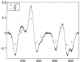
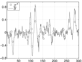
The sparse deconvolution problem takes the form ${\mathb{y}}={\mathb{h}}\ast{\mathb{x}}^{\star}+{\mathb{n}}$ where the impulse response $\mathb{h}$ is a Gaussian filter of standard deviation $\sigma$, and the noise $\mathb{n}$ is assumed i.i.d. and Gaussian. The problem rereads ${\mathb{y}}={\mathb{A}}{\mathb{x}}^{\star}+{\mathb{n}}$ where $\mathb{A}$ is a convolution matrix. In the default setting, $\mathb{y}$ and $\mathb{x}$ are sampled at the same frequency. $\mathb{h}$ is approximated by a finite impulse response of length $6\sigma$ by thresholding the smallest values. $\mathb{A}$ is a Toeplitz matrix of dimensions chosen so that any Gaussian feature ${\mathb{h}}\ast{\mathb{x}}^{\star}$ if fully contained within the observation window $\{1,\ldots,m\}$. This implies that $\mathb{A}$ is slightly undercomplete: $m>n$ with $m\approx n$. Two simulated data vectors $\mathb{y}$ are represented in Fig. 8(a,b) where ${\mathb{x}}^{\star}$ are $k$-sparse vectors with $k=10$ and 30, and the signal-to-noise ratio (SNR) is equal to 25 and 10 dB, respectively. It is defined by $\textrm{SNR}=10\,\log({\|{\mathb{A}}{\mathb{x}}^{\star}\|_{2}^{2}/(m\sigma_{n}^{2})})$ where $\sigma_{n}^{2}$ is the variance of the noise process $\mathb{n}$.

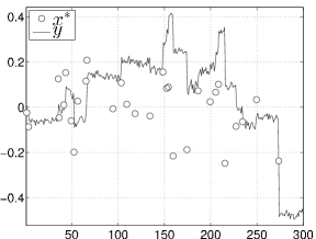
The jump detection problem is illustrated on Fig. 8(c,d). Here, $\mathb{A}$ is the squared dictionary ($m=n$) defined by $A_{i,j}=1$ if $i\geq j$, and 0 otherwise. The atom ${\mathb{a}}_{j}$ codes for a jump at location $j$, and $x_{j}^{\star}$ matches the height of the jump. When ${\mathb{x}}^{\star}$ is $k$-sparse, ${\mathb{A}}{\mathb{x}}^{\star}$ yields a piecewise constant signal with $k$ pieces, ${\mathb{x}}^{\star}$ being the first-order derivative of the signal ${\mathb{A}}{\mathb{x}}^{\star}$.

Both generic problems involve either square or slightly undercomplete dictionaries. The case of overcomplete dictionaries will be discussed as well, e.g., by considering the deconvolution problem with undersampled observations $\mathb{y}$. The generic problems are already difficult because neighboring columns of $\mathb{A}$ are highly correlated, and a number of fast algorithms that are efficient for well-conditioned dictionaries may fail to recover the support of ${\mathb{x}}^{\star}$. The degree of difficulty of the deconvolution problem is controlled by the width $\sigma$ of the Gaussian impulse response and the sparsity $k$: for large values of $k$ and/or $\sigma$, the Gaussian features resulting from the convolution ${\mathb{h}}\ast{\mathb{x}}^{\star}$ strongly overlap. For the jump detection problem, all the step signals related to the atoms ${\mathb{a}}_{j}$ have overlapping supports.

V-B Empirical behavior of CSBR and $\ell_{0}$-PD

V-B1 Example

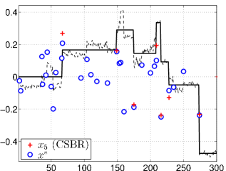
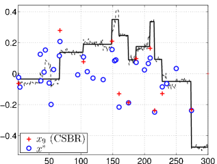
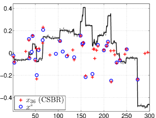
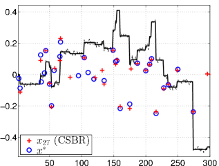
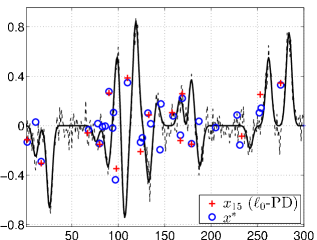
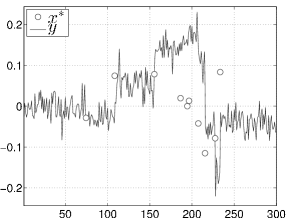
Consider the problem shown on Fig. 8(c). Because CSBR and $\ell_{0}$-PD provide very similar results, we only show the CSBR results. CSBR delivers sparse solutions ${\mathb{x}}_{j}$ for decreasing $\lambda_{j}$, ${\mathb{x}}_{j}$ being the least-square solution supported by the $j$-th output of CSBR ($S_{j}$). Three sparse solutions ${\mathb{x}}_{j}$ are represented on Fig. 9. For the first solution (lowest value of $|S_{j}|$, largest $\lambda_{j}$), only the seven main jumps are being detected (Fig. 9(a)). The cardinality of $S_{j}$ increases with $j$, and some other jumps are obtained together with possible false detections (Figs. 9(b,c)).

V-B2 Model order selection

It may often be useful to select a single solution ${\mathb{x}}_{j}$. The proposed algorithms are compatible with most classical methods of model order selection [46, 47] because they are greedy algorithms. Assuming that the variance of the observation noise is unknown, we distinguish two categories of cost functions for estimation of the order $\|{\mathb{x}}_{j}\|_{0}=|S_{j}|$. The first take the form $\min_{j}\{m\log{\mathcal{E}}(S_{j})+\alpha|S_{j}|\}$ where $\alpha$ equals 2, $\log m$, and $2\log\log m$ for the Akaike, Minimum Description Length (MDL) and Hannan and Quinn criteria, respectively [46]. The second are cross-validation criteria [48, 49]. The sparse approximation framework allows one to derive simplified expressions of the latter up to the storage of intermediate solutions of greedy algorithms for consecutive cardinalities [8, 47, 50].

(a)

(b)

Figure 10: Model order selection using MDLc: display of the selected sparse solution ${\mathb{x}}_{j}$ and the related data approximation signal. The data of Fig. 8(c,b) ($k=30$ true spikes) are processed using CSBR and $\ell_{0}$-PD, respectively. (a) corresponds to the simulation shown on Fig. 9. The MDLc solution is the CSBR output support $S_{27}$ of cardinality 27. (b) is related to the $\ell_{0}$-PD output $S_{15}$, with $|S_{15}|=16$.

(a)

(b)

Figure 11: Typical approximate $\ell_{0}$-curves found for the deconvolution problem of Fig. 8(a): zoom in for small and large $\lambda$’s. The $\ell_{0}$-PD curve is concave and continuous on $\lambda\in{\mathbbm{R}}_{+}$. The CSBR curve is continuous only for large $\lambda$-values (black circles). For low $\lambda$’s, there can be discontinuities at breakpoint locations (white circles). Here, both curves almost coincide for large $\lambda$’s. The $\ell_{0}$-PD curve lays below the CSBR curve for low $\lambda$’s.

For the sparse deconvolution and jump detection problems, we found that the Akaike and cross validation criteria severely over-estimate the expected number of spikes. On the contrary, the MDL criterion yields quite accurate results. We found that the modified MDLc version dedicated to short data records (i.e., when the number of observations is moderately larger than the model order) [51] yields the best results for all the scenarii we have tested. It reads:

$$\min_{j}\Bigl{\{}\log{\mathcal{E}}(S_{j})+\frac{\log(m)(|S_{j}|+1)}{m-|S_{j}|-2}\Bigr{\}}.$$ (15)

Fig. 10(a) illustrates that the number of spikes found using MDLc is very accurate for high SNRs (27 spikes are found, the unknown order being 30). It is underestimated for low SNRs: 16 spikes are found (instead of 30) for the simulation of Fig. 10(b) where $\textrm{SNR}=10$ dB. This behavior is relevant because for noisy data, the spikes of smallest amplitudes are drowned in the noise. One cannot expect to detect them.

V-B3 Further empirical observations

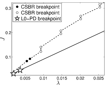
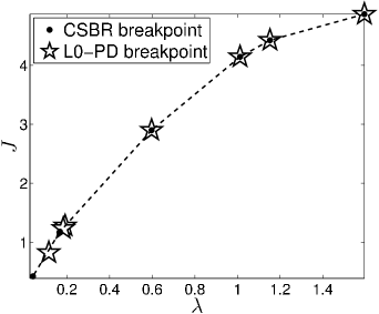
Fig. 11 is a typical display of the approximate $\ell_{0}$-curves yielded by CSBR and $\ell_{0}$-PD. The $\ell_{0}$-PD curve is structurally continuous and concave whereas for the CSBR curve, there are two kinds of breakpoints depicted with black and white circles. The former are “continuous” breakpoints. This occurs when no single replacement is done during the call to SBR ($\textrm{SBR}(S_{\mathrm{init}};\lambda_{j})$ returns $S_{j}=S_{\mathrm{init}}$; see Tab. II). Otherwise, a discontinuity breakpoint (white circle) appears. In Fig. 11, the CSBR and $\ell_{0}$-PD curves almost coincide for large $\lambda$’s, where only continuous breakpoints can be observed. For low $\lambda$’s, the $\ell_{0}$-PD curve lays below the CSBR curve, and discontinuity breakpoints appear in the latter curve.

(a) CSBR	(b) CSBR
(c) $\ell_{0}$-PD	(d) $\ell_{0}$-PD

Figure 12: Series of single replacements performed by CSBR and $\ell_{0}$-PD. (a) CSBR: cardinality of the current support found after each single replacement. (b) Breakpoints $\lambda_{j}$ found by CSBR, represented in log-scale. SBR is executed for each $\lambda_{j}$, and the number of single replacements for fixed $\lambda_{j}$ matches the length of the horizontal steps in the figure. (c) $\ell_{0}$-PD: cardinality of the supports appended to the regularization path during the iterations. At each iteration, 0, 1 or 2 supports are included. Vertical steps appear whenever two supports are simultaneously included. (d) $\ell_{0}$-PD: representation in log-scale of the current interval $(\lambda_{j+1},\lambda_{j})$ (grey color). When the grey bars reach the bottom of the image, the lower bound equals $\lambda_{j+1}=0$.

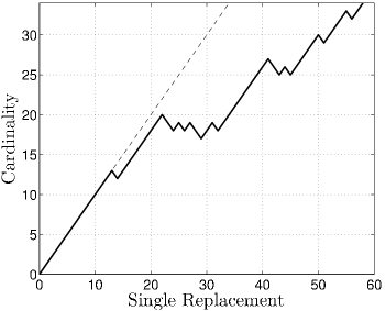
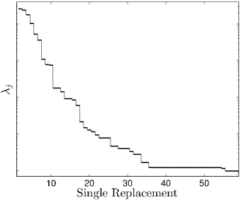
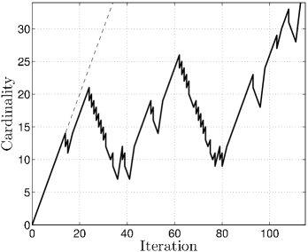
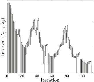
Fig. 12 provides some insight on the CSBR and $\ell_{0}$-PD iterations for a sparse deconvolution problem with $\|{\mathb{x}}^{\star}\|_{0}=17$ and $\textrm{SNR}=20$ dB. In the CSBR subfigures, the horizontal axis represents the number of single replacements: 60 replacements are being performed from the initial empty support during the successive calls to SBR. For $\ell_{0}$-PD, the horizontal axis shows the iteration number. At most two new supports are being included in the list of candidate subsets at each iteration. The number of effective single replacements is therefore increased by 0, 1 or 2. During the first 25 iterations, $\ell_{0}$-PD mainly operates atom selections similar to CSBR. The explored subsets are thus of increasing cardinality and $\lambda$ is decreasing (Figs. 12(c,d)). From iterations 25 to 40, the very sparse solutions previously found ($k\leq 20$) are improved as a series of atom de-selections is performed. They are being improved again around iteration 80. On the contrary, the sparsest solutions are never improved with CSBR, which works for decreasing $\lambda$’s (Figs. 12(a,b)). For $\ell_{0}$-PD, the early stopping parameter $\lambda_{\mathrm{stop}}$ may have a strong influence on the improvement of the sparsest solutions and the overall computation time. This point will be further discussed below.

V-C Extensive comparisons

The proposed algorithms are compared with popular nonconvex algorithms for both problems introduced in subsection V-A with various parameter settings: problem dimension ($m,n$), ratio $m/n$, signal-to-noise ratio, cardinality of ${\mathb{x}}^{\star}$, and width $\sigma$ of the Gaussian impulse response for the deconvolution problem. The settings are listed on Table V for 10 scenarii. Because the proposed algorithms are orthogonal greedy algorithms, they are better suited to problems in which the level of sparsity is moderate to high. We therefore restrict ourselves to the case where $k=\|{\mathb{x}}^{\star}\|_{0}\leq 30$.

TABLE V: Settings related to each scenario: $k$ is the sparsity. $f$ controls the dictionary size: $m=f\;m_{\mathrm{DEF}},\,n=f\;n_{\mathrm{DEF}}$ with $n_{\mathrm{DEF}}\approx m_{\mathrm{DEF}}=300$. By default, $f=1$. The undersampling parameter $\Delta$ equals 1 by default ($m_{\mathrm{DEF}}\geq n_{\mathrm{DEF}}$). It is increased to generate problems with overcomplete dictionaries ($m\approx n/\Delta$). The Gaussian impulse response width is set to $\sigma=f\;\sigma_{\mathrm{DEF}}$ with $\sigma_{\mathrm{DEF}}=3$ or 8.

Scenario	Type	SNR	$k$	$f$	$\Delta$	$m$	$n$	$\sigma$
A	Deconv.	25	30	1	1	300	282	3
B	Deconv.	10	10	1	1	300	252	8
C	Deconv.	25	10	3	1	900	756	24
D	Deconv.	25	30	6	1	1800	1692	18
E	Jumps	25	10	1	1	300	300	$\emptyset$
F	Jumps	25	30	1	1	300	300	$\emptyset$
G	Jumps	10	10	1	1	300	300	$\emptyset$
H	Deconv.	$+\infty$	10	3	2	450	756	24
I	Deconv.	$+\infty$	30	3	2	450	756	24
J	Deconv.	$+\infty$	10	1	4	75	252	8

V-C1 Competing algorithms

We focus on the comparison with algorithms based on nonconvex penalties. It is indeed increasingly acknowledged that the BPDN estimates are less accurate than sparse approximation estimates based on nonconvex penalties. We do not consider forward greedy algorithms either; we already showed that SBR is (unsurprisingly) more efficient than the simpler OMP and OLS algorithms [3]. Among the popular nonconvex algorithms, we consider:

1. Iterative Reweighted Least Squares (IRLS) for $\ell_{q}$ minimization, $q<1$ [52];

2. Iterative Reweighted $\ell_{1}$ (IR$\ell_{1}$) coupled with the penalty $\log(|x_{i}|+\varepsilon)$ [53, 20, 23];

3. $\ell_{0}$ penalized least squares for cyclic descent (L0LS-CD) [54];

4. Smoothed $\ell_{0}$ (SL0) [43, 55].

We resort to a penalized least-square implementation for all algorithms, the only algorithm directly working with the $\ell_{0}$ penalty being L0LS-CD. We do not consider simpler thresholding algorithms (Iterative Hard Thresholding, CoSaMP, Subspace Pursuit) proposed in the context of compressive sensing since we found that SBR behaves much better than these algorithms for ill-conditioned dictionaries [3]. We found that L0LS-CD is more efficient than thresholding algorithms. Moreover, the cyclic descent approach is becoming very popular in the recent sparse approximation literature [44, 56] although its speed of convergence is sensitive to the quality of the initial solution. Here, we use the BPDN initial solution $\mathop{\mathrm{arg\,min}}_{\mathb{x}}\,\{\|{\mathb{y}}-{\mathb{A}}{\mathb{x}}\|_{2}^{2}+\mu\|{\mathb{x}}\|_{1}\}$ where $\mu$ is set to half of the maximum tested $\lambda$-value (more details will be given hereafter). This simple ad hoc setting allows us to get a rough initial solution that is nonzero and very sparse within a fast computation time.

The three other considered algorithms work with sparsity measures depending on an arbitrary parameter. Regarding IRLS, we set $q=0.5$ or 0.1 as suggested in [52]. We chose to run IRLS twice, with $q=0.5$ and then $q=0.1$ (with the previous output at $q=0.5$ as initial solution) so that IRLS is less sensitive to local solutions at $q=0.1$. SL0 is a GNC-like algorithm working for increasingly non-convex penalties (i.e., Gaussian functions of decreasing widths). For simplicity reasons, we set the lowest width relative to the knowledge of the smallest nonzero amplitude of the ground truth solution ${\mathb{x}}^{\star}$. The basic SL0 implementation is dedicated to noise-free problems [43]. There exist several adaptations in the noisy setting [55, 57] including the precursory work [58]. We chose the efficient implementation of [57] in which the original pseudo-inverse calculations are replaced by a quasi-Newton strategy using limited memory BFGS updates. Finally, the IR$\ell_{1}$ implementation depends on both the choice of parameter $\varepsilon$ (which controls the degree of nonconvexity) and the $\ell_{1}$ solver. We have tested two $\ell_{1}$ solvers: the in-crowd algorithm [59] together with an empirical setting of $\varepsilon>0$, and $\ell_{1}$ homotopy in the limit case $\varepsilon\rightarrow 0$, following [53]. We found that $\ell_{1}$ homotopy is faster than in-crowd, mainly because the Matlab implementation of in-crowd (provided by the authors) makes calls to the quadprog built-in function, which is computationally expensive for large dimension problems.

V-C2 Numerical protocol

Because the competing algorithms work for a single $\lambda$ value, we need to define a grid, denoted by $\{\lambda_{i}^{\mathrm{G}},\,i=1,\ldots,N_{\lambda}\}$, for comparison purposes. Such grid is defined in logscale for each of the 10 scenarii $(k,{\mathb{A}},\mathrm{SNR})$ defined in Table V. The number of grid points is $N_{\lambda}=11$. For a given scenario, $T=30$ trials are being performed in which $k$-sparse vectors ${\mathb{x}}^{\star}(t)$ and noise vector ${\mathb{n}}(t)$ are randomly drawn. This leads us to simulate $T$ observation vectors ${\mathb{y}}(t)={\mathb{A}}{\mathb{x}}^{\star}(t)+{\mathb{n}}(t)$ with $t\in\{1,\ldots,T\}$. Specifically, the location of the nonzero amplitudes in ${\mathb{x}}^{\star}(t)$ are uniformly distributed and the amplitude values are drawn according to an i.i.d. Gaussian distribution. For each trial $t$, all competing algorithms need to be run $N_{\lambda}$ times with ${\mathb{y}}(t)$ and $\lambda_{i}^{\mathrm{G}}$ as inputs whereas CSBR and $\ell_{0}$-PD are run only once since they deliver estimates for a continuum of values of $\lambda$. Their solution for each $\lambda_{i}^{\mathrm{G}}$ directly deduces from their set of output supports and the knowledge of both breakpoints surrounding $\lambda_{i}^{\mathrm{G}}$.

$\min_{\mathb{x}}{\mathcal{J}}({\mathb{x}};\lambda)$	CPU Time (seconds)	$\min_{\mathb{x}}{\mathcal{J}}({\mathb{x}};\lambda)$	CPU Time (seconds)
(A)	(A)	(B)	(B)
(C)	(C)	(D)	(D)

Figure 13: Comparison of algorithms for the noisy deconvolution problem, i.e., for the first scenarii reported on Table V. For each scenario, the algorithms are being evaluated in terms of ${\mathcal{J}}$-value and of CPU time for $N_{\lambda}=11$ values $\lambda_{i}^{\mathrm{G}}$. Evaluations are averaged over 30 trials. The overall and mean (normalization by $N_{\lambda}=11$) CPU times related to CSBR (respectively, $\ell_{0}$-PD) are shown as two parallel horizontal lines.

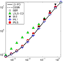
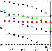
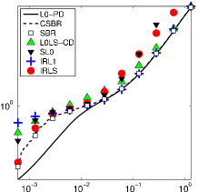
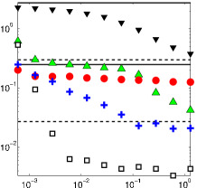
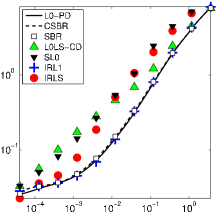
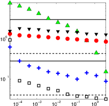
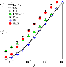
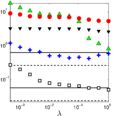
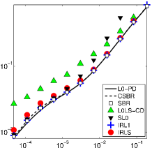
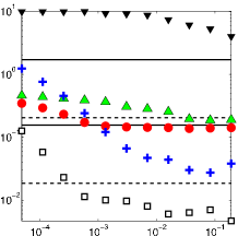
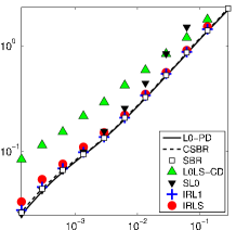
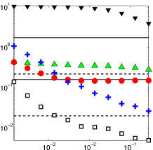
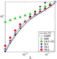
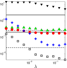
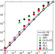
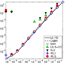
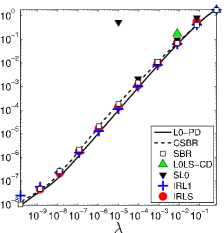
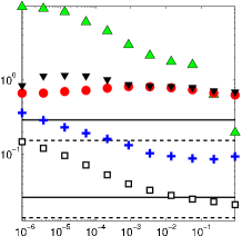
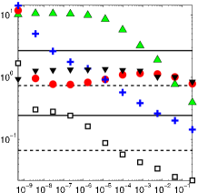
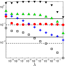
The algorithms are first evaluated in the optimization viewpoint: the related criteria are their capacity to reach a low value of ${\mathcal{J}}({\mathb{x}};\lambda)$ and the corresponding CPU time. In this viewpoint, the proposed methods might be somehow favored since they are more directly designed with the criterion ${\mathcal{J}}({\mathb{x}};\lambda)$ in mind. On the other hand, ${\mathcal{J}}({\mathb{x}};\lambda)$ appears to be a natural indicator because solving either $\ell_{0}$-minimization problem (1), (2) or (3) is the ultimate goal of any sparse approximation method. As detailed below, some post-processing will be applied to the outputs of algorithms that do not rely on the $\ell_{0}$-norm so that they are not strongly disadvantaged. Practically, we store the value of ${\mathcal{J}}({\mathb{x}};\lambda_{i}^{\mathrm{G}})$ found for each trial and each $\lambda_{i}^{\mathrm{G}}$. Averaging this value over the trials $t$ yields a table $\textrm{TabJ}(a,\lambda_{i}^{\mathrm{G}})$ where $a$ denotes a candidate algorithm. Similarly, the CPU time is averaged over the trials $t$, leading to another table $\textrm{TabCPU}(a,\lambda_{i}^{\mathrm{G}})$. Each table is represented separately as a 2D plot with a specific color for each algorithm: see, e.g., Fig. 13. CSBR and $\ell_{0}$-PD are represented with continuous curves because ${\mathcal{J}}({\mathb{x}};\lambda)$ is computed for a continuum of $\lambda$’s, and the CPU time is computed only once.

The algorithms are also evaluated in terms of support recovery accuracy. For this purpose, let us first define the “support error” as the minimum over $i$ of the distance

$$|S^{\star}(t)\backslash S(t,a,\lambda_{i}^{\mathrm{G}})|+|S(t,a,\lambda_{i}^{\mathrm{G}})\backslash S^{\star}(t)|$$ (16)

between the support $S^{\star}(t)$ of the unknown sparse vector ${\mathb{x}}^{\star}(t)$ and the support $S(t,a,\lambda_{i}^{\mathrm{G}})$ of the sparse reconstruction at $\lambda_{i}^{\mathrm{G}}$ with algorithm $a$. (16) takes into account both numbers of false negatives $|S^{\star}(t)\backslash S(t,a,\lambda_{i}^{\mathrm{G}})|$ and of false positives $|S(t,a,\lambda_{i}^{\mathrm{G}})\backslash S^{\star}(t)|$. Denoting by $S(t,a,\lambda_{\mathrm{opt}}^{\mathrm{G}})\leftarrow S(t,a,\lambda_{i}^{\mathrm{G}})$ the solution support that is the closest to $S^{\star}(t)$ according to (16), we further consider the number of true positives in $S(t,a,\lambda_{\mathrm{opt}}^{\mathrm{G}})$, defined as $|S^{\star}(t)\cap S(t,a,\lambda_{\mathrm{opt}}^{\mathrm{G}})|$. We will thus report:

• the support error;

• the corresponding number of true positives;

• the corresponding model order $|S(t,a,\lambda_{\mathrm{opt}}^{\mathrm{G}})|$.

Averaging these measures over $T$ trials yields the support error score SE($a$), the true positive score TP($a$) and the model order, denoted by Order($a$). The numbers of false positives (FP) and of true/false negatives can be directly deduced, e.g., FP($a$) $=$ Order($a$) $-$ TP($a$).

The underlying idea in this analysis is that when SE is small (respectively, TP is high), the algorithms are likely to perform well provided that $\lambda$ is appropriately chosen. However, in practical applications, only one estimate is selected using a suitable model selection criterion. We therefore provide additional evaluations of the MDLc estimate accuracy. For CSBR and $\ell_{0}$-PD, all output supports are considered to compute the MDLc estimate as described in subsection V-B. For other algorithms, it is equal to one of the sparse reconstructions obtained at $\lambda_{i}^{\mathrm{G}}$ for $i\in\{1,\ldots,N_{\lambda}\}$. The same three measures as above are computed for the MDLc estimate and averaged over $T$ trials. They are denoted by MDLc-SE($a$), MDLc-TP($a$) and MDLc-Order($a$).

V-C3 Technical adaptations for comparison purposes

Because IRLS and SL0 do not deliver sparse vectors in the strict sense, it is necessary to sparsify their outputs before computing their SE($a$) score. This is done by running one iteration of cyclic descent (L0LS-CD): most small nonzero amplitudes are then thresholded to 0. Regarding the values of ${\mathcal{J}}({\mathb{x}};\lambda)$, a post-processing is performed for algorithms that do not rely on the $\ell_{0}$-norm. This post-processing can be interpreted as a local descent of ${\mathcal{J}}({\mathb{x}};\lambda)$. It consists in: (i) running one iteration of cyclic descent (L0LS-CD); (ii) computing the squared error related to the output support. L0LS-CD is indeed a local descent algorithm dedicated to ${\mathcal{J}}({\mathb{x}};\lambda)$ but the convergence towards a least-square minimizer is not reached in one iteration.

$\min_{\mathb{x}}{\mathcal{J}}({\mathb{x}};\lambda)$	CPU Time (seconds)	$\min_{\mathb{x}}{\mathcal{J}}({\mathb{x}};\lambda)$	CPU Time (seconds)
(E)	(E)	(F)	(F)
(G)	(G)

Figure 14: Comparison of algorithms for the jump detection problem for the scenarii E, F and G of Table V.

V-C4 Analysis in the optimization viewpoint

CSBR and $\ell_{0}$-PD are always among the most accurate to minimize the cost function, as illustrated on Figs. 13, 14 and 15. We can clearly distinguish two groups of algorithms on these figures: IRLS, L0LS-CD and SL0 one the one hand, and the OLS-based algorithms (SBR, CSBR, $\ell_{0}$-PD) and IR$\ell_{1}$ on the other hand, which are the most accurate. We cannot clearly discriminate the accuracy of SBR and CSBR: one may behave slightly better than the other depending on the scenarii. On the contrary, SBR and CSBR are often outperformed by $\ell_{0}$-PD. The obvious advantage of CSBR and $\ell_{0}$-PD over SBR and IR$\ell_{1}$ is that they are $\ell_{0}$-homotopy algorithms, i.e., a set of solutions are delivered for many sparsity levels, and the corresponding $\lambda$-values are adaptively found. On the contrary, the SBR output is related to a single $\lambda$ whose tuning may be tricky. Another advantage over IR$\ell_{1}$ is that the structure of forward-backward algorithms is simpler, as no call to any $\ell_{1}$ solver is required. Moreover, the number of parameters to tune is lower: there is a single (early) stopping parameter $\lambda_{\mathrm{stop}}$.

The price to pay for a better performance is an increase of the computation burden. On Figs. 13, 14 and 15, two lines are drawn for CSBR (respectively, for $\ell_{0}$-PD). They are horizontal because the algorithm is run only once per trial, so there is a single computation time measurement. The first line corresponds to the overall computation time, i.e., from the start to the termination of CSBR / $\ell_{0}$-PD. This time is often more expensive than for other algorithms. However, the latter times refer to a single execution for some $\lambda_{i}^{\mathrm{G}}$ value. If one wants to recover sparse solutions for many $\lambda_{i}^{\mathrm{G}}$’s, they must be cumulated. This is the reason why we have drawn a second line for CSBR and $\ell_{0}$-PD corresponding to a normalization (by $N_{\lambda}=11$) of the overall computation time. In this viewpoint, the CPU time of CSBR and $\ell_{0}$-PD are very reasonable.

TABLE VI: Jump detection problem in the noisy setting. The algorithms are evaluated in terms of support error (SE) and number of true positives (TP). The number of jumps that are found is reported (Order) together with the “true order” corresponding to the ground truth $k$. The scores related to the MDLc estimate are indicated similarly.

Scenario E	$\ell_{0}$-PD	CSBR	SBR	$\ell_{0}$LS-CD	S$\ell_{0}$	IR$\ell_{1}$	IRLS
SE	1.6	1.6	1.6	5.3	4.0	1.5	1.8
TP	8.6	8.7	8.6	5.2	7.8	8.7	8.7
Order (true: 10)	8.8	9.0	8.9	5.7	9.6	8.9	9.1
MDLc-SE	4.7	4.3	4.1	22.7	5.6	4.1	3.5
MDLc-TP	8.7	8.8	8.8	6.9	8.6	8.8	8.8
MDLc-Order	12.2	11.9	11.6	26.6	12.7	11.7	11.0
Scenario F	$\ell_{0}$-PD	CSBR	SBR	$\ell_{0}$LS-CD	S$\ell_{0}$	IR$\ell_{1}$	IRLS
SE	11.1	11.9	11.8	22.5	11.6	10.9	11.6
TP	21.2	20.6	20.7	9.2	20.3	20.8	20.7
Order (true: 30)	23.6	23.2	23.2	10.9	22.2	22.5	23.1
MDLc-SE	13.7	13.4	13.4	39.2	14.0	13.1	13.3
MDLc-TP	21.8	21.8	21.4	12.9	21.6	22.1	21.5
MDLc-Order	27.3	27.0	26.3	35.0	27.2	27.2	26.4
Scenario G	$\ell_{0}$-PD	CSBR	SBR	$\ell_{0}$LS-CD	S$\ell_{0}$	IR$\ell_{1}$	IRLS
SE	7.3	7.5	7.5	8.9	10.3	7.2	7.5
TP	4.0	3.6	3.6	3.1	2.9	3.9	4.0
Order (true: 10)	5.23	4.73	4.73	5.17	6.07	4.97	5.57
MDLc-SE	11.4	10.7	10.9	11.7	15.1	11.2	10.7
MDLc-TP	4.2	4.2	4.2	3.0	3.9	4.2	4.4
MDLc-Order	9.8	9.1	9.3	7.6	12.8	9.6	9.5

The computation time depends on many factors among which the implementation of algorithms (including the memory storage) and the chosen stopping rules. We have followed an homogeneous implementation of algorithms to make the CPU time comparisons meaningful. We have defined two sets of stopping rules depending on the problem dimension. The default parameters apply to medium size problems ($m=300$). They are relaxed for problems of larger dimension ($m>500$) to avoid huge computational costs. The stopping rule of CSBR and $\ell_{0}$-PD is always $\lambda\leq\lambda_{\mathrm{stop}}=\alpha\lambda_{1}^{\mathrm{G}}$ with $\alpha=1$ for CSBR and 0.5 (medium size) or 0.8 (large size) for $\ell_{0}$-PD. For L0LS-CD, the maximum number of cyclic descents (update of every amplitude $x_{i}$) is set to 60 or 10 depending on the dimension. For SL0, we have followed the default setting of [43] for the rate of deformation of the nonconvex penalty. The number of BFGS iterations done in the local minimization steps for each penalty is set to $L=$ 40 or 5. It is set to $5L$ for the last penalty which is the most nonconvex. Regarding IRLS and IRL$\ell_{1}$, we keep the same settings whatever the dimension since the computation times remain reasonable for large dimensions. Finally, SBR does not require any arbitrary stopping rule. The problems of large dimensions correspond to scenarii C and D. We observe on Fig. 13 that the comparison (trade-off performance vs computation time) is now clearly in favor of CSBR and $\ell_{0}$-PD. IR$\ell_{1}$ remains very competitive although the average numerical cost becomes larger.

(H)	(I)	(J)

Figure 15: Comparison of algorithms for the noise-free deconvolution problem, i.e., for the scenarii H, I and J of Table V. Some markers do not appear for low $\lambda$’s (L0LS-CD, SL0) in the left figures because they do not lay in the zoom-in window (their performance is poor).

V-C5 Analysis in the support recovery viewpoint

The support recovery performance is only shown for the scenarii E to J (Tabs. VI and VII). For noisy deconvolution problems, these results are omitted because the support error is often quite large and the true positive scores are low whatever the algorithm, especially for scenarii B to D. Specifically, the least support error always exceeds 20, 10, 10 and 32 for the scenarii A to D ($k=30$, 10, 10 and 30, respectively). For such difficult problems, one can hardly discriminate algorithms based on simple binary tests such as the true positive rate. More sophisticated localization tests are non binary and would take into account the distance between the location of the true spikes and their wrong estimates [60]. It is noticeable, though, that the MDLc estimator delivers subsets of realistic cardinality for scenarii A to D (e.g., the subsets found with CSBR are of cardinalities 33, 9, 15 and 38, the true cardinalities being 30, 10, 10 and 30). The model orders are also quite accurate for the noisy jump detection problem (Tab. VI) whereas the true support is often partially detected by several of the considered algorithms. Here, CSBR and $\ell_{0}$-PD are among the best algorithms in terms of support error.

The results of Tab. VII and Fig. 15 correspond to the deconvolution problem in noise-free case. The data $\mathb{y}$ are undersampled so that the dictionary $\mathb{A}$ is overcomplete. The undersampling rate $\Delta\approx m/n$ is set to 2 in scenarii H and I and 4 in scenario J. Again, CSBR and $\ell_{0}$-PD are among the best (SE, TP, MDLc-order) especially for the most difficult problem J.

TABLE VII: Sparse deconvolution problem in the noise-free setting: exact support recovery.

Scenario H	$\ell_{0}$-PD	CSBR	SBR	$\ell_{0}$LS-CD	S$\ell_{0}$	IR$\ell_{1}$	IRLS
SE	2.5	3.6	4.8	11.4	13.0	0.8	6.1
TP	8.3	8.2	6.8	0.4	0.1	9.5	9.4
Order (true: 10)	9.1	10.0	8.3	2.2	3.2	9.8	14.9
MDLc-SE	3.6	3.8	5.8	168.5	343.8	1.1	9.0
MDLc-TP	8.6	8.6	7.9	3.3	6.6	9.5	9.6
MDLc-Order	10.8	11.0	11.6	153.5	347.0	10.1	18.2
Scenario I	$\ell_{0}$-PD	CSBR	SBR	$\ell_{0}$LS-CD	S$\ell_{0}$	IR$\ell_{1}$	IRLS
SE	0.9	1.3	2.1	36.7	48.5	3.8	9.4
TP	29.4	29.3	29.1	0.7	0.8	28.0	27.7
Order (true: 30)	29.7	29.8	30.2	8.2	20.1	29.8	34.8
MDLc-SE	3.8	3.5	3.7	686.0	444.9	9.5	114.3
MDLc-TP	29.5	29.4	29.2	28.6	17.5	28.5	26.4
MDLc-Order	32.8	32.3	32.1	437.0	449.8	36.5	137.2
Scenario J	$\ell_{0}$-PD	CSBR	SBR	$\ell_{0}$LS-CD	S$\ell_{0}$	IR$\ell_{1}$	IRLS
SE	0.3	3.5	5.3	10.3	10.4	2.4	4.3
TP	9.8	7.3	5.8	0.6	2.6	8.8	9.2
Order (true: 10)	9.8	8.1	6.9	1.4	5.6	10.0	12.7
MDLc-SE	2.6	7.7	12.4	176.2	78.6	7.2	69.0
MDLc-TP	9.7	8.9	8.0	8.6	3.0	8.9	4.1
MDLc-Order	12.0	15.5	18.5	73.0	74.6	14.9	67.2

V-C6 Overcomplete dictionaries with noise

We now provide arguments indicating that the proposed algorithms are competitive as well for noisy problems with overcomplete dictionaries. The detailed experiments commented below are not reported for space reasons.

We have first considered the noisy deconvolution problem with $\Delta=2$ or 4 leading to overcomplete dictionaries, the other parameters being set as in scenarii A to D. Although the data approximation is qualitatively good for CSBR and $\ell_{0}$-PD, the SE and TP scores are very weak. It is hard to discriminate the performance of algorithms because these measures are very weak for all considered algorithms. Moreover, the values of ${\mathcal{J}}(\lambda)$ found for most algorithms are often similar.

We have also considered an adaptive spline approximation problem generalizing the jump detection problem to the approximation of a signal using piecewise polynomials of degree $P=1$ or 2 [3]. The jump detection problem can indeed be thought of as the approximation with a piecewise constant signal ($P=0$). The generalized version [3] is inspired from the regression spline modeling in [61]. Now, the dictionary atoms are related to the detection of the locations of jumps, changes of slopes and changes of curvatures in the signal $\mathb{y}$ (subdictionaries ${\mathb{A}}^{0}$, ${\mathb{A}}^{1}$ and ${\mathb{A}}^{2}$). The dictionary then takes the form ${\mathb{A}}\leftarrow[{\mathb{A}}^{0},{\mathb{A}}^{1}]$ or ${\mathb{A}}\leftarrow[{\mathb{A}}^{0},{\mathb{A}}^{1},{\mathb{A}}^{2}]$ where each sub-dictionary ${\mathb{A}}^{p}$ ($p\leq P$) is formed of shifted versions of the one-sided power function $i\mapsto[\max(i,0)]^{p}$. The size of the full dictionary ${\mathb{A}}$ is approximately $m\times(P+1)m$. Hence, it becomes overcomplete as soon as $P\geq 1$. We have shown [3] that SBR is competitive when $P=1$ or 2. We have carried out new tests confirming that CSBR and $\ell_{0}$-PD are more efficient than their competitors in terms of values of ${\mathcal{J}}(\lambda)$. However, the rate of true positives is low for $P\geq 1$ since the location of the change of slopes and of curvatures can hardly be exactly recovered from noisy data.

VI Software

The Matlab implementation of the proposed CSBR and $\ell_{0}$-PD algorithms is available at
www.cran.univ-lorraine.fr/perso/charles.soussen/software.html including programs showing how to call these functions.

VII Conclusion

The choice of a relevant sparse approximation algorithm relies on a trade-off between the desired performance and the computation time one is ready to spend. The proposed algorithms are relatively expensive but very well suited to inverse problems inducing highly correlated dictionaries. A reason is that they have the capacity to escape from local minimizers of ${\mathcal{J}}({\mathb{x}};\lambda)=\|{\mathb{y}}-{\mathb{A}}{\mathb{x}}\|_{2}^{2}+\lambda\|{\mathb{x}}\|_{0}$ [3]. This behavior is in contrast with other classical sparse algorithms.

We have shown the usefulness and efficiency of the two SBR extensions when the level of sparsity is moderate to high, i.e., $k/\min(m,n)$ is lower than 0.1. They remain competitive when $k/\min(m,n)$ ranges between 0.1 and 0.2, and their performance gradually degrade for weaker levels of sparsity, which is an expected behavior for such greedy type algorithms. For a single $\lambda$, CSBR is as efficient as SBR, and $\ell_{0}$-PD improves the SBR and CSBR performance within a larger computation cost. The main benefit over SBR is that sparse solutions are provided for a continuum of $\lambda$-values, enabling the utilization of any classical order selection method. We found that the MDL criterion yields very accurate estimates of the cardinality $\|{\mathb{x}}\|_{0}$.

Our perspectives include the proposal of forward-backward search algorithms that will be faster than SBR and potentially more efficient. In the standard version of SBR, CSBR and $\ell_{0}$-PD, a single replacement refers to the insertion or removal of a dictionary element. The cost of an iteration is essentially related to the $n$ linear system resolutions done to test single replacements for all dictionary atoms. The proposed algorithms obviously remain valid when working with a larger neighborhood, e.g., when testing the replacement of two atoms simultaneously, but their complexity becomes huge. To avoid such numerical explosion, one may rather choose not to carry out all the replacement tests, but only some tests that are likely to be effective. Extensions of OMP and OLS were recently proposed in this spirit [36] and deserve consideration for proposing efficient forward-backward algorithms.

Appendix A Properties of the $\ell_{0}$ regularization paths

In this appendix, we prove that the $\ell_{0}$-penalized path ${\mathcal{S}}^{\star}_{\mathrm{P}}$ (see Definition 2) is piecewise constant (Theorem 1) and is a subset of the $\ell_{0}$-constrained regularization path ${\mathcal{S}}^{\star}_{\mathrm{C}}$ (Theorem 2). We will denote the $\ell_{0}$-curve by $\lambda\mapsto{\mathcal{J}}^{\star}(\lambda)=\min_{S}\{\hat{{\mathcal{J}}}(S;\lambda)\}$. Let us recall that this function is concave and affine on each interval $(\lambda_{i+1}^{\star},\lambda_{i}^{\star})$, with $i\in\{0,\ldots,I\}$ (Definition 1). Moreover, $\lambda_{I+1}^{\star}=0$ and $\lambda_{0}^{\star}=+\infty$.

A-A Proof of Theorem 1

We prove Theorem 1 together with the following lemma, which is informative about the content of ${\mathcal{S}}^{\star}_{\mathrm{P}}(\lambda)$ for the breakpoints $\lambda=\lambda_{i}^{\star}$.

Lemma 2

Let $i\in\{1,\ldots,I-1\}$. Then, for all $\lambda\in(\lambda_{i+1}^{\star},\lambda_{i}^{\star})$, ${\mathcal{S}}^{\star}_{\mathrm{P}}(\lambda)\subset{\mathcal{S}}^{\star}_{\mathrm{P}}(\lambda^{\star}_{i+1})\cap{\mathcal{S}}^{\star}_{\mathrm{P}}(\lambda^{\star}_{i})$.

For the first and last intervals, we have:

• For all $\lambda\in(0,\lambda_{I}^{\star})$, ${\mathcal{S}}^{\star}_{\mathrm{P}}(\lambda)\subset{\mathcal{S}}^{\star}_{\mathrm{P}}(\lambda^{\star}_{I})$.

• For all $\lambda\in(\lambda_{1}^{\star},+\infty)$, ${\mathcal{S}}^{\star}_{\mathrm{P}}(\lambda)=\{\emptyset\}\subset{\mathcal{S}}^{\star}_{\mathrm{P}}(\lambda_{1}^{\star})$.

Proof:

By definition, the $\ell_{0}$-curve is the concave envelope of the (finite) set of lines $S$ for all possible subsets $S$. Because it is affine on the $i$-th interval $(\lambda^{\star}_{i+1},\lambda^{\star}_{i})$, ${\mathcal{J}}^{\star}(\lambda)$ coincides with $\hat{{\mathcal{J}}}({S_{i}};\lambda)={\mathcal{E}}(S_{i})+\lambda|S_{i}|$, where $S_{i}$ is some optimal subset for all $\lambda\in(\lambda^{\star}_{i+1},\lambda^{\star}_{i})$.

Let $\lambda\in(\lambda^{\star}_{i+1},\lambda^{\star}_{i})$ and $S\in{\mathcal{S}}^{\star}_{\mathrm{P}}(\lambda)$. Then, $\hat{{\mathcal{J}}}(S;\lambda)=\hat{{\mathcal{J}}}({S_{i}};\lambda)$. It follows that both lines $S$ and $S_{i}$ necessarily coincide; otherwise, they would intersect at $\lambda$, and line $S$ would lay below $S_{i}$ on either interval $(\lambda^{\star}_{i+1},\lambda)$ or $(\lambda,\lambda^{\star}_{i})$, which contradicts the definition of $S_{i}$. We conclude that $S\in{\mathcal{S}}^{\star}_{\mathrm{P}}(\lambda^{\prime})$ for all $\lambda^{\prime}\in(\lambda^{\star}_{i+1},\lambda^{\star}_{i})$.

We have shown that the content of ${\mathcal{S}}^{\star}_{\mathrm{P}}(\lambda)$ does not depend on $\lambda$ when $\lambda\in(\lambda^{\star}_{i+1},\lambda^{\star}_{i})$. ∎

Proof:

The first result ${\mathcal{S}}^{\star}_{\mathrm{P}}(\lambda)\subset{\mathcal{S}}^{\star}_{\mathrm{P}}(\lambda^{\star}_{i+1})\cap{\mathcal{S}}^{\star}_{\mathrm{P}}(\lambda^{\star}_{i})$ is obtained by slightly adapting the proof of Theorem 1: replace $(\lambda^{\star}_{i+1},\lambda^{\star}_{i})$ by the closed interval $[\lambda^{\star}_{i+1},\lambda^{\star}_{i}]$, and set $\lambda^{\prime}$ to both endpoints of this interval.

The second and third results are obtained similarly, by considering the intervals $(0,\lambda^{\star}_{I}]$ and $[\lambda^{\star}_{1},+\infty)$, and setting $\lambda^{\prime}\leftarrow\lambda^{\star}_{I}$ and $\lambda^{\prime}\leftarrow\lambda^{\star}_{1}$, respectively. It is obvious that ${\mathcal{S}}^{\star}_{\mathrm{P}}(\lambda)$ reduces to the empty support for $\lambda>\lambda_{1}^{\star}$ since the $\ell_{0}$-curve is constant for $\lambda>\lambda_{1}^{\star}$. ∎

A-B Proof of Theorem 2

The first result is straightforward: for any $\lambda$ and for $S\in{\mathcal{S}}^{\star}_{\mathrm{P}}(\lambda)$, we have $S\in{\mathcal{S}}^{\star}_{\mathrm{C}}(|S|)$. Otherwise, there would exist $S^{\prime}$ with $|S^{\prime}|\leq|S|$ and ${\mathcal{E}}(S^{\prime})<{\mathcal{E}}(S)$. Then, $\hat{{\mathcal{J}}}({S^{\prime}};\lambda)<\hat{{\mathcal{J}}}({S};\lambda)$ would contradict $S\in{\mathcal{S}}^{\star}_{\mathrm{P}}(\lambda)$.

To prove the second result, let us first show that for any $i$, $\exists k_{i}:\,\forall\lambda\in(\lambda^{\star}_{i+1},\lambda^{\star}_{i}),\,{\mathcal{S}}^{\star}_{\mathrm{P}}(\lambda)\subset{\mathcal{S}}^{\star}_{\mathrm{C}}(k_{i})$.

Let $S\in{\mathcal{S}}^{\star}_{\mathrm{P}}(\lambda)$ for some $\lambda\in(\lambda^{\star}_{i+1},\lambda^{\star}_{i})$. Theorem 1 implies that $S\in{\mathcal{S}}^{\star}_{\mathrm{P}}(\lambda)$ for any $\lambda\in(\lambda^{\star}_{i+1},\lambda^{\star}_{i})$. Therefore, ${\mathcal{J}}^{\star}(\lambda)=\hat{{\mathcal{J}}}(S;\lambda)$ for $\lambda\in(\lambda^{\star}_{i+1},\lambda^{\star}_{i})$, and the slope of line $S$, i.e., $|S|$, is constant whatever $S\in{\mathcal{S}}^{\star}_{\mathrm{P}}(\lambda)$ and $\lambda\in(\lambda^{\star}_{i+1},\lambda^{\star}_{i})$. Let us denote this constant by $k_{i}=|S|$. According to the first paragraph of the proof, $S\in{\mathcal{S}}^{\star}_{\mathrm{P}}(\lambda)$ implies that $S\in{\mathcal{S}}^{\star}_{\mathrm{C}}(k_{i})$.

Let us prove the reverse inclusion ${\mathcal{S}}^{\star}_{\mathrm{C}}(k_{i})\subset{\mathcal{S}}^{\star}_{\mathrm{P}}(\lambda)$. Let $\lambda\in(\lambda^{\star}_{i+1},\lambda^{\star}_{i})$ and $S\in{\mathcal{S}}^{\star}_{\mathrm{C}}(k_{i})$. First, we have $|S|\leq k_{i}$. Second, for any $S^{\prime}\in{\mathcal{S}}^{\star}_{\mathrm{P}}(\lambda)$, we have $|S^{\prime}|=k_{i}$ by definition of $k_{i}$. We also have that ${\mathcal{E}}(S^{\prime})={\mathcal{E}}(S)$ because ${\mathcal{S}}^{\star}_{\mathrm{P}}(\lambda)\subset{\mathcal{S}}^{\star}_{\mathrm{C}}(k_{i})$. Finally, $\hat{{\mathcal{J}}}(S^{\prime};\lambda)\geq\hat{{\mathcal{J}}}({S};\lambda)$. $S^{\prime}\in{\mathcal{S}}^{\star}_{\mathrm{P}}(\lambda)$ implies that $S\in{\mathcal{S}}^{\star}_{\mathrm{P}}(\lambda)$. This concludes the proof of the second result.

References

- [1] B. K. Natarajan, “Sparse approximate solutions to linear systems”, SIAM J. Comput., vol. 24, no. 2, pp. 227–234, Apr. 1995.
- [2] M. Nikolova, “Description of the minimizers of least squares regularized with norm. Uniqueness of the global minimizer”, SIAM J. Imaging Sci., vol. 6, no. 2, pp. 904–937, May 2013.
- [3] C. Soussen, J. Idier, D. Brie, and J. Duan, “From Bernoulli-Gaussian deconvolution to sparse signal restoration”, IEEE Trans. Signal Process., vol. 59, no. 10, pp. 4572–4584, Oct. 2011.
- [4] J. A. Tropp and S. J. Wright, “Computational methods for sparse solution of linear inverse problems”, Proc. IEEE, invited paper (Special Issue “Applications of sparse representation and compressive sensing”), vol. 98, no. 5, pp. 948–958, June 2010.
- [5] S. Mallat and Z. Zhang, “Matching pursuits with time-frequency dictionaries”, IEEE Trans. Signal Process., vol. 41, no. 12, pp. 3397–3415, Dec. 1993.
- [6] Y. C. Pati, R. Rezaiifar, and P. S. Krishnaprasad, “Orthogonal matching pursuit: Recursive function approximation with applications to wavelet decomposition”, in Proc. 27th Asilomar Conf. on Signals, Systems and Computers, Nov. 1993, vol. 1, pp. 40–44.
- [7] S. Chen, S. A. Billings, and W. Luo, “Orthogonal least squares methods and their application to non-linear system identification”, Int. J. Control, vol. 50, no. 5, pp. 1873–1896, Nov. 1989.
- [8] A. J. Miller, Subset selection in regression, Chapman and Hall, London, UK, 2nd edition, Apr. 2002.
- [9] S. F. Cotter, J. Adler, B. D. Rao, and K. Kreutz-Delgado, “Forward sequential algorithms for best basis selection”, IEE Proc. Vision, Image and Signal Processing, vol. 146, no. 5, pp. 235–244, Oct. 1999.
- [10] L. Rebollo-Neira and D. Lowe, “Optimized orthogonal matching pursuit approach”, IEEE Signal Process. Lett., vol. 9, no. 4, pp. 137–140, Apr. 2002.
- [11] T. Blumensath and M. E. Davies, “Iterative thresholding for sparse approximations”, J. Fourier Anal. Appl., vol. 14, no. 5, pp. 629–654, Dec. 2008.
- [12] W. Dai and O. Milenkovic, “Subspace pursuit for compressive sensing signal reconstruction”, IEEE Trans. Inf. Theory, vol. 55, no. 5, pp. 2230–2249, May 2009.
- [13] D. Needell and J. A. Tropp, “CoSaMP: Iterative signal recovery from incomplete and inaccurate samples”, Appl. Comp. Harmonic Anal., vol. 26, no. 3, pp. 301–321, May 2009.
- [14] C. Herzet and A. Drémeau, “Bayesian pursuit algorithms”, Research Report, INRIA Rennes Bretagne Atlantique - Télécom ParisTech, Rennes, France, Jan. 2014.
- [15] M. A. Efroymson, “Multiple regression analysis”, in Mathematical Methods for Digital Computers, A. Ralston and H. S. Wilf, Eds., vol. 1, pp. 191–203. Wiley, New York, 1960.
- [16] K. N. Berk, “Forward and backward stepping in variable selection”, J. Statist. Comput. Simul., vol. 10, no. 3-4, pp. 177–185, Apr. 1980.
- [17] T. Zhang, “Adaptive forward-backward greedy algorithm for learning sparse representations”, IEEE Trans. Inf. Theory, vol. 57, no. 7, pp. 4689–4708, July 2011.
- [18] M. A. T. Figueiredo, R. D. Nowak, and S. J. Wright, “Gradient projection for sparse reconstruction: Application to compressed sensing and other inverse problems”, IEEE J. Sel. Top. Signal Process., vol. 1, no. 4, pp. 586–597, Dec. 2007.
- [19] M. Zibulevsky and M. Elad, “ optimization in signal and image processing”, IEEE Sig. Proc. Mag., vol. 27, no. 3, pp. 76–88, May 2010.
- [20] E. J. Candès, M. B. Wakin, and S. P. Boyd, “Enhancing sparsity by reweighted minimization”, J. Fourier Anal. Appl., vol. 14, no. 5-6, pp. 877–905, Dec. 2008.
- [21] G. Gasso, A. Rakotomamonjy, and S. Canu, “Recovering sparse signals with a certain family of nonconvex penalties and DC programming”, IEEE Trans. Signal Process., vol. 57, no. 12, pp. 4686–4698, Dec. 2009.
- [22] N. Mourad and J. P. Reilly, “Minimizing nonconvex functions for sparse vector reconstruction”, IEEE Trans. Signal Process., vol. 58, no. 7, pp. 3485–3496, July 2010.
- [23] D. P. Wipf and S. Nagarajan, “Iterative reweighted and methods for finding sparse solutions”, IEEE J. Sel. Top. Signal Process. (Special issue on Compressive Sensing), vol. 4, no. 2, pp. 317–329, Apr. 2010.
- [24] A. Gholami and S. M. Hosseini, “A general framework for sparsity-based denoising and inversion”, IEEE Trans. Signal Process., vol. 59, no. 11, pp. 5202–5211, Nov. 2011.
- [25] I. Ramírez and G. Sapiro, “Universal regularizers for robust sparse coding and modeling”, IEEE Trans. Image Process., vol. 21, no. 9, pp. 3850–3864, Sept. 2012.
- [26] H. A. Le Thi, B. T. Nguyen Thi, and H. M. Le, “Sparse signal recovery by difference of convex functions algorithms”, in Intelligent Information and Database Systems, A. Selamat, N. T. Nguyen, and H. Haron, Eds., Berlin, 2013, vol. 7803 of Lecture Notes in Computer Science, pp. 387–397, Springer Verlag.
- [27] I. Selesnick and I. Bayram, “Sparse signal estimation by maximally sparse convex optimization”, IEEE Trans. Signal Process., vol. 62, no. 5, pp. 1078–1092, Mar. 2014.
- [28] D. L. Donoho and Y. Tsaig, “Fast solution of -norm minimization problems when the solution may be sparse”, IEEE Trans. Inf. Theory, vol. 54, no. 11, pp. 4789–4812, Nov. 2008.
- [29] M. R. Osborne, B. Presnell, and B. A. Turlach, “A new approach to variable selection in least squares problems”, IMA Journal of Numerical Analysis, vol. 20, no. 3, pp. 389–403, 2000.
- [30] B. Efron, T. Hastie, I. Johnstone, and R. Tibshirani, “Least angle regression”, Ann. Statist., vol. 32, no. 2, pp. 407–499, Apr. 2004.
- [31] I. Das and J. E. Dennis, “A closer look at drawbacks of minimizing weighted sums of objectives for Pareto set generation in multicriteria optimization problems”, Structural optimization, vol. 14, no. 1, pp. 63–69, Aug. 2007.
- [32] R. T. Marler and J. S. Arora, “Survey of multi-objective optimization methods for engineering”, Structural and Multidisciplinary Optimization, vol. 26, no. 6, pp. 369–395, Apr. 2004.
- [33] E. van den Berg and M. P. Friedlander, “Probing the Pareto frontier for basis pursuit solutions”, SIAM J. Sci. Comput., vol. 31, no. 2, pp. 890–912, Nov. 2008.
- [34] P. M. T. Broersen, “Subset regression with stepwise directed search”, J. R. Statist. Soc. C, vol. 35, no. 2, pp. 168–177, 1986.
- [35] D. Haugland, “A bidirectional greedy heuristic for the subspace selection problem”, in Engineering stochastic local search algorithms. Designing, implementing and analyzing effective heuristics, T. Stützle, M. Birattari, and H. H. Hoos, Eds., Berlin, Germany, Sept. 2007, vol. 4638 of Lect. Notes Comput. Sci., pp. 162–176, Springer Verlag.
- [36] S. Chatterjee, D. Sundman, M. Vehkaperä, and M. Skoglund, “Projection-based and look-ahead strategies for atom selection”, IEEE Trans. Signal Process., vol. 60, no. 2, pp. 634–647, Feb. 2012.
- [37] J. Duan, C. Soussen, D. Brie, and J. Idier, “A continuation approach to estimate a solution path of mixed L2-L0 minimization problems”, in Signal Processing with Adaptive Sparse Structured Representations (SPARS workshop), Saint-Malo, France, Apr. 2009, pp. 1–6.
- [38] S. Kwon, J. Wang, and B. Shim, “Multipath matching pursuit”, IEEE Trans. Inf. Theory, vol. 60, no. 5, pp. 2986–3001, May 2014.
- [39] S. Maymon and Y. Eldar, “The Viterbi algorithm for subset selection”, IEEE Signal Process. Lett., vol. 22, no. 5, pp. 524–528, May 2015.
- [40] E. Wasserstrom, “Numerical solutions by the continuation method”, SIAM Rev., vol. 15, no. 1, pp. 89–119, Jan. 1973.
- [41] D. M. Malioutov, M. Çetin, and A. S. Willsky, “Homotopy continuation for sparse signal representation”, in Proc. IEEE ICASSP, Philadephia, PA, Mar. 2005, vol. V, pp. 733–736.
- [42] J. Trzasko and A. Manduca, “Highly undersampled magnetic resonance image reconstruction via homotopic -minimization”, IEEE Trans. Medical Imaging, vol. 8, no. 1, pp. 106–121, Jan. 2009.
- [43] G. H. Mohimani, M. Babaie-Zadeh, and C. Jutten, “A fast approach for overcomplete sparse decomposition based on smoothed norm”, IEEE Trans. Signal Process., vol. 57, no. 1, pp. 289–301, Jan. 2009.
- [44] R. Mazumder, J. H. Friedman, and T. Hastie, “SparseNet: Coordinate descent with nonconvex penalties”, J. Acoust. Soc. Amer., vol. 106, no. 495, pp. 1125–1138, Sept. 2011.
- [45] D. L. Donoho, V. Stodden, and Y. Tsaig, “About SparseLab”, Tech. Rep., Stanford University, Mar. 2007.
- [46] P. Stoica and Y. Selén, “Model-order selection: a review of information criterion rules”, IEEE Sig. Proc. Mag., vol. 21, no. 4, pp. 36–47, July 2004.
- [47] Y. Wang, “Model selection”, in Handbook of Computational Statistics, J. E. Gentle, W. Härdle, and Y. Mori, Eds., Berlin, Aug. 2004, vol. 1, pp. 437–466, Springer-Verlag.
- [48] G. Wahba, “Practical approximate solutions to linear operator equations when the data are noisy”, SIAM J. Num. Anal., vol. 14, no. 4, pp. 651–667, 1977.
- [49] G. H. Golub, M. Heath, and G. Wahba, “Generalized cross-validation as a method for choosing a good ridge parameter”, Technometrics, vol. 21, no. 2, pp. 215–223, May 1979.
- [50] C. D. Austin, R. L. Moses, J. N. Ash, and E. Ertin, “On the relation between sparse reconstruction and parameter estimation with model order selection”, IEEE J. Sel. Top. Signal Process., vol. 4, no. 3, pp. 298–309, June 2010.
- [51] F. de Ridder, R. Pintelon, J. Schoukens, and D. P. Gillikin, “Modified AIC and MDL model selection criteria for short data records”, IEEE Trans. Instrum. and Meas., vol. 54, no. 1, pp. 144–150, Feb. 2005.
- [52] M.-J. Lai, Y. Xu, and W. Yin, “Improved iteratively reweighted least squares for unconstrained smoothed minimization”, SIAM J. Num. Anal., vol. 51, no. 2, pp. 927–957, Mar. 2013.
- [53] H. Zou, “The adaptive Lasso and its oracle properties”, J. Acoust. Soc. Amer., vol. 101, no. 476, pp. 1418–1429, Dec. 2006.
- [54] A. J. Seneviratne and V. Solo, “Sparse coloured system identification with guaranteed stability”, in IEEE Conference on Decision and Control, Honolulu, HI, Dec. 2012, pp. 2826–2831.
- [55] A. Eftekhari, M. Babaie-Zadeh, C. Jutten, and H. A. Moghaddam, “Robust-sl0 for stable sparse representation in noisy settings”, in Proc. IEEE ICASSP, Taipei, Taiwan, Apr. 2009, pp. 3433–3436.
- [56] G. Marjanovic and V. Solo, “ sparsity penalized linear regression with cyclic descent”, IEEE Trans. Signal Process., vol. 62, no. 6, pp. 1464–1475, Mar. 2014.
- [57] X. Ye, W.-P. Zhu, A. Zhang, and J. Yan, “Sparse channel estimation of mimo-ofdm systems with unconstrained smoothed -norm-regularized least squares compressed sensing”, EURASIP J. Wireless Comm. and Networking, vol. 2013, no. 282, pp. 1–13, Dec. 2013.
- [58] N. Saito, “Superresolution of noisy band-limited data by data adaptive regularization and its application to seismic trace inversion”, in Proc. IEEE ICASSP, Albuquerque, NM, Apr. 1990, pp. 1237–1240.
- [59] P. R. Gill, A. Wang, and A. Molnar, “The in-crowd algorithm for fast basis pursuit denoising”, IEEE Trans. Signal Process., vol. 59, no. 10, pp. 4595–4605, Oct. 2011.
- [60] M. C. van Rossum, “A novel spike distance”, Neural Computation, vol. 13, no. 4, pp. 751–763, Apr. 2001.
- [61] J. H. Friedman, “Multivariate adaptive regression splines”, Ann. Statist., vol. 19, no. 1, pp. 1–67, Mar. 1991.