Reverse Time Migration for Reconstructing Extended Obstacles in Planar Acoustic Waveguides

Abstract

We propose a new reverse time migration method for reconstructing extended obstacles in the planar waveguide using acoustic waves at a fixed frequency. We prove the resolution of the reconstruction method in terms of the aperture and the thickness of the waveguide. The resolution analysis implies that the imaginary part of the cross-correlation imaging function is always positive and thus may have better stability properties. Numerical experiments are included to illustrate the powerful imaging quality and to confirm our resolution results.

1 Introduction

We propose a reverse time migration (RTM) method to find the support of an unknown obstacle embedded in a planar acoustic waveguide from the measurement of the wave field on part of the boundary of the waveguide which is far away from the obstacle (see Figure 1). Let ${\mathbb{R}}^{2}_{h}=\{(x_{1},x_{2})\in{\mathbb{R}}^{2}:x_{2}\in(0,h)\}$ be the waveguide of thickness $h>0$. Denote by $\Gamma_{0}=\{(x_{1},x_{2})\in{\mathbb{R}}^{2}:x_{2}=0\}$ and $\Gamma_{h}=\{(x_{1},x_{2})\in{\mathbb{R}}^{2}:x_{2}=h\}$ the boundaries of ${\mathbb{R}}^{2}_{h}$. Let the obstacle occupy a bounded Lipschitz domain $D$ included in $B_{R}=(-R,R)\times(0,h)$, $R>0$, with $\nu$ the unit outer normal to its boundary $\Gamma_{D}$. We assume the incident wave is a point source excited at $x_{s}\in\Gamma_{h}$. The measured wave field satisfies the following equations:

$$\Delta u+k^{2}u=-\delta_{x_{s}}(x)\qquad\mbox{in }{\mathbb{R}}^{2}_{h}\backslash\bar{D},$$ (1)

$$\frac{\partial u}{\partial\nu}+\mathbf{i}k\eta(x)u=0\ \ \ \ \mbox{ on }\Gamma_{D},$$ (2)

$$u=0\ \ \mbox{on }\Gamma_{0},\ \ \ \ \frac{\partial u}{\partial x_{2}}=0\ \ \mbox{on }\Gamma_{h}.$$ (3)

Here $k>0$ is the wave number and $\eta(x)>0$ is a bounded function on $\Gamma_{D}$. The equation (1) is understood as the limit when $x_{s}\in{\mathbb{R}}^{2}_{h}\backslash\bar{D}$ tends to $\Gamma_{h}$. The impedance boundary condition in (2) is assumed only for the convenience of the analysis of this paper. The RTM method studied in this paper does not require any a priori information of the physical properties of the obstacle such as penetrable and non-penetrable, and for the non-penetrable obstacles, the type of boundary conditions on the boundary of the obstacle (see section 6 below).

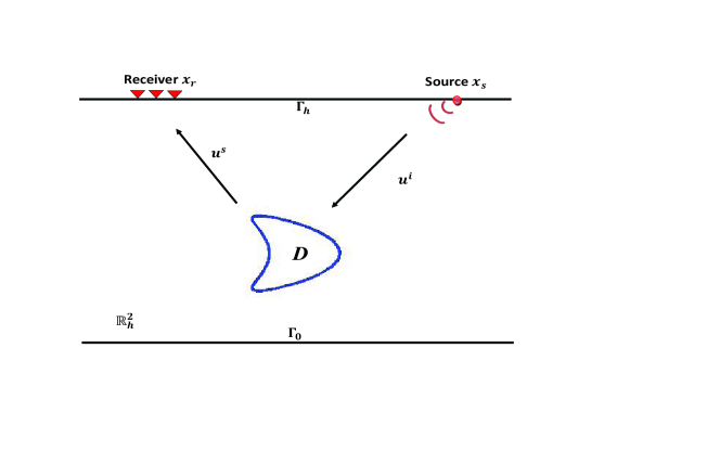
Fig. 1: The geometric setting of the inverse problem in planar waveguides.

Now we introduce the radiation condition for the planar waveguide problem [27]. Since $D\subset B_{R}$, we have by separation of variables the following mode expansion:

$$u(x_{1},x_{2})=\sum_{n=1}^{\infty}u_{n}(x_{1})\sin(\mu_{n}x_{2}),\ \ \ \ \forall\ |x_{1}|>R,$$ (4)

where $\mu_{n}=\frac{2n-1}{2h}\pi$, $n=1,2,\cdots$, are called cut-off frequencies. In this paper we will always assume

$$k\not=\frac{2n-1}{2h}\pi,\ \ n=1,2,\cdots.$$ (5)

The mode expansion coefficients $u_{n}(x_{1})$, $n=1,2,\cdots$, satisfy the 1D Helmholtz equation:

$$u_{n}^{\prime\prime}+\xi_{n}^{2}u_{n}=0,\ \ \ \ \forall\ |x_{1}|>R,\ \ n=1,2,...,$$ (6)

where $\xi_{n}=\sqrt{k^{2}-\mu_{n}^{2}}$ if $k>\mu_{n}$ and $\xi_{n}=\mathbf{i}\sqrt{\mu_{n}^{2}-k^{2}}$ if $k<\mu_{n}$. The radiation condition for the planar waveguide problem is then to impose the mode expansion coefficient $u_{n}(x_{1})$ to satisfy

$$\lim_{|x_{1}|\to\infty}\bigg{(}\frac{\partial u_{n}}{\partial|x_{1}|}-\mathbf{i}\xi_{n}u_{n}\bigg{)}=0,\ \ n=1,2,\cdots,$$ (7)

which guarantees the uniqueness of the solution of the 1D Helmholtz equation (6). The existence and uniqueness of the wave scattering problem (1)-(3) with the radiation condition (7) is an intensively studied subject in the literature, see e.g. [2, 20, 21, 22, 27]. The difficulty is the possible existence of the so-called embedded trapped modes which destroys the uniqueness of the solution [19]. In this paper we will show that the impedance boundary condition on the scatterer guarantees the uniqueness of the scattering solution. We also prove the existence of the solution by the limiting absorption principle.

It is well known that imaging a scatterer in a waveguide is much more challenging than in the free space. Indeed, because of the presence of two parallel infinite boundaries of the waveguide, only a finite number of modes can propagate at long distance, while the other modes decay exponentially [27]. We refer to [1] for MUSIC type algorithm to locate small inclusions, [28] for the generalized dual space method, [3, 6, 24] for the linear sampling method, [25] for a selective imaging method based on Kirchhoff migration, and the inversion method in [23] for reconstructing obstacles in waveguides.

The RTM method, which consists of back-propagating the complex conjugated data into the background medium and computing the cross-correlation between the incident wave field and the backpropagation field to output the final imaging profile, is nowadays widely used in exploration geophysics [4, 13, 5]. In [10, 11], the RTM method for reconstructing extended targets using acoustic and electromagnetic waves at a fixed frequency in the free space is proposed and studied. The resolution analysis in [10, 11] is achieved without using the small inclusion or geometrical optics assumption previously made in the literature.

The purpose of this paper is to extend the RTM method in [10, 11] to find extended targets in the planar acoustic waveguide. Our new RTM algorithm is motivated by a generalized Helmholtz-Kirchhoff identity for the waveguide scattering problems. We show our new imaging function enjoys the nice feature that it is always positive and thus may have better stability properties. The key ingredient in the analysis is a decay estimate of the difference of the Green function for the waveguide problem and the half space Green function. We also refer to [17] for the study of the resolution of time-reversal experiments.

The rest of this paper is organized as follows. In section 2 we introduce some necessary results concerning the direct scattering problem. In section 3 we prove the generalized Helmholtz-Kirchhoff identity and introduce our RTM algorithm. In section 4 we study the resolution of the finite aperture Helmholtz-Kirchhoff function which plays a key role in the resolution analysis of RTM algorithm in section 5. In section 6 we consider the extension of the resolution results for reconstructing penetrable obstacles or non-penetrable obstacles with sound soft or sound hard boundary conditions. In section 7 we report extensive numerical experiments to show the competitive performance of the RTM algorithm. In section 8 we include some concluding remarks. The appendix is devoted to the proof of the existence of the solution of the direct scattering problem by the limiting absorption principle.

2 Direct scattering problem

We start by introducing the Green function $N(x,y)$, where $y\in{\mathbb{R}}^{2}_{h}$, which is the radiation solution satisfying the equations:

$$\Delta N(x,y)+k^{2}N(x,y)=-\delta_{y}(x)\qquad\mbox{ in }{\mathbb{R}}^{2}_{h},$$

$$N(x,y)=0\ \ \mbox{on }\Gamma_{0},\ \ \ \ \frac{\partial N(x,y)}{\partial x_{2}}=0\ \ \mbox{on }\Gamma_{h}.$$

Let $\hat{N}_{y}(\xi,x_{2})=\int^{\infty}_{-\infty}N(x,y)e^{-\mathbf{i}(x_{1}-y_{1})\xi}dx_{1}$ be the Fourier transform in the first variable. It is easy to find by the assumption that $N(x,y)$ is a radiation solution that

$$\hat{N}_{y}(\xi,x_{2})=\frac{\textbf{i}}{2\mu}\bigg{(}e^{\textbf{i}\mu|x_{2}-y_{2}|}-e^{\textbf{i}\mu(x_{2}+y_{2})}-\frac{2\sin(\mu x_{2})}{\cos(\mu h)}\sin(\mu y_{2})e^{\textbf{i}\mu h}\bigg{)},$$ (8)

where $\mu=\sqrt{k^{2}-\xi^{2}}$ and we choose the branch cut of $\sqrt{z}$ such that $\mathrm{Re}\,(\sqrt{z})\geq 0$ throughout the paper. By using the limiting absorption principle one can obtain the following formula for the Green function by taking the inverse Fourier transform on the Sommerfeld Integral Path (SIP) (see Figure 2):

$${}N(x,y)=\frac{1}{2\pi}\int_{\rm SIP}\hat{N}_{y}(\xi,x_{2})e^{\textbf{i}\xi(x_{1}-y_{1})}d\xi.$$ (9)

We refer to [12, Chapter 2] for more discussion on the SIPs. We will also use the following well-known normal mode expression for the Green function $N(x,y)$, see e.g. [27]:

$${}N(x,y)=\sum_{n=1}^{\infty}\frac{{\mathbf{i}}}{h\xi_{n}}\sin(\mu_{n}x_{2})\sin(\mu_{n}y_{2})e^{\mathbf{i}\xi_{n}|x_{1}-y_{1}|}.$$ (10)

It is obvious that the series in the normal mode expression is absolutely convergent if $x_{1}\not=y_{1}$. If $x_{1}=y_{1}$ but $x_{2}\not=y_{2}$, the series in (10) is also convergent by using the method of Dirichlet’s test [26, §8.B.13-15].

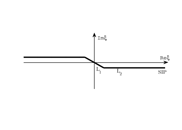
Fig. 2: The Sommerfeld Integral Path (SIP).

Lemma 1.

If $|x_{1}-y_{1}|\geq\alpha h$ for some constant $\alpha>0$, then $N(x,y)$ and ${\rm NewA}_{x}N(x,y)$ are uniformly bounded.

Proof.

We only prove $N(x,y)$ is uniformly bounded. The proof for ${\rm NewA}_{x}N(x,y)$ is similar. Let $M$ be the integer such that $\mu_{M}<k<\mu_{M+1}$. Since $\frac{e^{-\alpha kh\sqrt{t^{2}-1}}}{\sqrt{t^{2}-1}}$ is a decreasing function in $(1,\infty)$, we know that

$$\sum_{n=M+1}^{\infty}\frac{1}{h|\xi_{n}|}e^{-|\xi_{n}||x_{1}-y_{1}|}\leq\frac{1}{h|\xi_{M+1}|}+\frac{1}{\pi}\int^{\infty}_{1}\frac{e^{-\alpha kh\sqrt{t^{2}-1}}}{\sqrt{t^{2}-1}}dt\leq\frac{1}{h|\xi_{M+1}|}+\frac{1}{\alpha kh\pi}.$$

On the other hand, note that $|\sum_{n=1}^{M}\frac{\mathbf{i}}{h\xi_{n}}\sin(\mu_{n}x_{2})\sin(\mu_{n}y_{2})e^{\mathbf{i}\xi_{n}|x_{1}-y_{1}|}|<\sum_{n=1}^{M}\frac{1}{h\xi_{n}}$, we obtain

$$\sum_{n=1}^{M}\frac{1}{h\xi_{n}}\leq\frac{1}{h|\xi_{M}|}+\sum^{M-1}_{n=1}\frac{1}{h\xi_{n}}\leq\frac{1}{h|\xi_{M}|}+\frac{1}{\pi}\int_{0}^{1}\frac{1}{\sqrt{1-t^{2}}}dt=\frac{1}{h|\xi_{M}|}+\frac{1}{2},$$

where we have used the fact that $\frac{1}{\sqrt{1-t^{2}}}$ is an increasing function in $(0,1)$. This completes the proof.   ∎

Now we consider the existence and uniqueness of the radiation solution of the following waveguide problem:

$$\Delta\psi+k^{2}\psi=0\qquad\mbox{in }{\mathbb{R}}^{2}_{h}\backslash\bar{D},$$ (11)

$$\frac{\partial\psi}{\partial\nu}+\mathbf{i}k\eta(x)\psi=g\ \ \ \ \mbox{ on }\Gamma_{D},$$ (12)

$$\psi=0\ \ \mbox{on }\Gamma_{0},\ \ \ \ \frac{\partial\psi}{\partial x_{2}}=0\ \ \mbox{on }\Gamma_{h},$$ (13)

where $g\in H^{-1/2}(\Gamma_{D})$. We first show the uniqueness of the solution.

Lemma 2.

Let $\eta>0$ be bounded on $\Gamma_{D}$. The scattering problem (11)-(13) has at most one radiation solution.

Proof.

We include a proof here for the sake of completeness. Let $g=0$ in (12). We multiply (11) by $\bar{\psi}$ and integrate over $B_{R}\backslash\bar{D}$ to obtain by integration by parts that

$$-\mathrm{Im}\,\int_{\Gamma_{D}}\bar{\psi}\frac{\partial\psi}{\partial\nu}ds+\mathrm{Im}\,\int_{\partial B_{R}}\bar{\psi}\frac{\partial\psi}{\partial\nu}ds=0,$$ (14)

where $\nu$ is the unit outer normal to $\partial B_{R}$ on $\partial B_{R}$ and to $\Gamma_{D}$ on $\Gamma_{D}$. By the boundary condition satisfied by $\psi$, $\int_{(\Gamma_{0}\cup\Gamma_{h})\cap\partial B_{R}}\bar{\psi}\frac{\partial\psi}{\partial\nu}ds=0$. On the other hand, for $|x_{1}|>R$, similar to (4) we have the mode expansion $\psi(x)=\sum^{\infty}_{n=1}\psi_{n}(x_{1})\sin(\mu_{n}x_{2})$ with $\psi_{n}(x_{1})$ satisfying (6)-(7). Thus there exist constants $\psi_{n}^{\pm}$ such that $\psi_{n}(x_{1})=\psi_{n}^{\pm}e^{\mathbf{i}\xi_{n}|x_{1}|}$ for $\pm\,x_{1}>R$. By the Parseval identity, we have then

$$\int_{\Gamma_{R}^{+}\bigcup\Gamma_{R}^{-}}\bar{\psi}\frac{\partial\psi}{\partial\nu}ds=\frac{h}{2}\sum_{n=1}^{M}\mathbf{i}\xi_{n}(|\psi_{n}^{+}|^{2}+|\psi_{n}^{-}|^{2})-\frac{h}{2}\sum_{n=M+1}^{+\infty}|\xi_{n}|(|\psi_{n}^{+}|^{2}+|\psi_{n}^{-}|^{2})e^{-2|\xi_{n}|R},$$

where $\Gamma_{R}^{\pm}=\{(x_{1},x_{2})\in{\mathbb{R}}^{2}:x_{1}=\pm R,x_{2}\in(0,h)\}.$ Thus by taking the imaginary part of the above identity and inserting it into (14) we have

$$-\mathrm{Im}\,{\int_{\Gamma_{D}}\bar{\psi}\frac{\partial\psi}{\partial\nu}ds}+\frac{h}{2}\sum_{n=1}^{M}\xi_{n}(|\psi_{n}^{+}|^{2}+|\psi_{n}^{-}|^{2})=0.$$ (15)

By using the impedance condition and the assumption $\eta>0$ on $\Gamma_{D}$ we have $\psi=0$ on $\Gamma_{D}$ and $\psi_{n}^{\pm}=0,n=1,2,...,M$. This implies that $\frac{\partial\psi}{\partial\nu}=0$ on $\Gamma_{D}$. By the unique continuation principle we conclude $\psi=0$ in ${\mathbb{R}}^{2}_{h}\backslash\bar{D}$. This completes the proof.   ∎

In this paper, we call $\psi_{n}^{\pm},n=1,2,\cdots,M$, which are the coefficients of the propagating modes, the far-field pattern of the radiation solution $\psi$ of the planar waveguide problem (11)-(13).

We remark that under some assumption on the geometry of the obstacle, the uniqueness of the solution to the acoustic waveguide scattering problem for the sound soft obstacle was first proved in [20] based on the Rellich type identity. The proof was refined in [22] and was also used in Arens [2] for 3D scattering problems. For general geometry of the obstacle, the embedded trapped mode may appear which makes the uniqueness fail [19].

The following theorem which is useful in our resolution analysis for the RTM algorithm will be proved in the Appendix by using the method of limiting absorption principle.

Theorem 3.

Let $g\in H^{-1/2}(\Gamma_{D})$ and $\eta(x)>0$ be bounded on $\Gamma_{D}$. Then the problem (11)-(13) admits a unique radiation solution $\psi\in H^{1}_{\rm loc}({\mathbb{R}}^{2}_{h}\backslash\bar{D})$ . Moreover, for any bounded open set $\mathcal{O}\subset{\mathbb{R}}^{2}\backslash\bar{D}$, there exists a constant $C$ such that $\|\psi\|_{H^{1}(\mathcal{O})}\leq C\|g\|_{H^{-1/2}(\Gamma_{D})}$.

3 The reverse time migration algorithm

In this section we develop the reverse time migration type algorithm for inverse scattering problems in the planar acoustic waveguide. Let $G(x,y)$ be the half-space Green function, where $y\in{\mathbb{R}}^{2}_{+}=\{(x_{1},x_{2})\in{\mathbb{R}}^{2}:x_{2}>0\}$, which satisfies the Sommerfeld radiation condition and the following equations:

$$\Delta G(x,y)+k^{2}G(x,y) = -\delta_{y}(x)\qquad\mbox{ in }{\mathbb{R}}_{+}^{2},$$

$$G(x,y) = 0\qquad\qquad\ \ \ \mbox{on }\Gamma_{0}.$$

It is well known by the image method that

$$G(x,y)=\frac{\textbf{i}}{4}H_{0}^{(1)}(k|x-y|)-\frac{\textbf{i}}{4}H_{0}^{(1)}(k|x-y^{\prime}|),$$ (16)

where $H^{(1)}_{0}(z)$ is the first Hankel function of zeroth order and $y^{\prime}=(y_{1},-y_{2})$ is the image point of $y=(y_{1},y_{2})$ with respect to $y_{2}=0$.

We start by proving the generalized Helmholtz-Kirchhoff identity which plays a key role in this paper.

Lemma 4.

Let $S(x,y)=N(x,y)-G(x,y)$. Then we have

$$\int_{\Gamma_{h}}\frac{\partial G(x,\zeta)}{\partial\zeta_{2}}\overline{N(\zeta,y)}ds(\zeta)=2\mathbf{i}\,\mathrm{Im}\,N(x,y)-S(x,y),\ \ \ \ \forall x,y\in{\mathbb{R}}^{2}_{h}.$$ (17)

Proof.

Let $x,y\in B_{R}=(-R,R)\times(0,h)$ for some $R>0$. Since $\mathrm{Im}\,G(x,\cdot)$ satisfies the Helmholtz equation, by the integral representation formula we obtain

$$\mathrm{Im}\,G(x,y)=\int_{\partial B_{R}}\left(\frac{\partial\,\mathrm{Im}\,G(x,\zeta)}{\partial\nu(\zeta)}N(\zeta,y)-\frac{\partial N(\zeta,y)}{\partial\nu(\zeta)}\mathrm{Im}\,G(x,\zeta)\right)ds(\zeta).$$

Again by the integral representation formula we have

$$\int_{\partial B_{R}}\left(\frac{\partial G(x,\zeta)}{\partial\nu(\zeta)}N(\zeta,y)-\frac{\partial N(\zeta,y)}{\partial\nu(\zeta)}G(x,\zeta)\right)ds(\zeta)=-N(x,y)+G(x,y)=-S(x,y).$$

Thus, since $\mathrm{Im}\,G(x,y)=\frac{1}{2\mathbf{i}}(G(x,y)-\overline{G(x,y)})$, we have

$$2\mathbf{i}\,\mathrm{Im}\,G(x,y)+S(x,y) = -\int_{\partial B_{R}}\left(\frac{\partial\overline{G(x,\zeta)}}{\partial\nu(\zeta)}N(\zeta,y)-\frac{\partial N(\zeta,y)}{\partial\nu(\zeta)}\overline{G(x,\zeta)}\right)ds(\zeta)$$ (18)

$$= -\int_{\Gamma_{h}\cap\partial B_{R}}\frac{\partial\overline{G(x,\zeta)}}{\partial\nu(\zeta)}N(\zeta,y)ds(\zeta)$$

$$- \int_{\Gamma^{\pm}_{R}}\left(\frac{\partial\overline{G(x,\zeta)}}{\partial\nu(\zeta)}N(\zeta,y)-\frac{\partial N(\zeta,y)}{\partial\nu(\zeta)}\overline{G(x,\zeta)}\right)ds(\zeta),$$

where we have used $\frac{\partial N(\zeta,y)}{\partial\nu(\zeta)}=0$ on $\Gamma_{h}$ and $G(x,\zeta)=N(\zeta,y)=0$ on $\Gamma_{0}$. By (16) we know that $|G(x,\zeta)|=O(|x-\zeta|^{-1/2})$ and $|\frac{\partial G(x,\zeta)}{\partial\zeta_{1}}|=O(|x-\zeta|^{-1/2})$ as $|x-\zeta|\to\infty$. Therefore, by using Lemma 1 we conclude that the integral on $\Gamma^{\pm}_{R}$ in (18) vanishes as $R\to\infty$. This shows by letting $R\to\infty$ that

$$2\mathbf{i}\,\mathrm{Im}\,G(x,y)+S(x,y)=-\int_{\Gamma_{h}}\frac{\partial\overline{G(x,\zeta)}}{\partial\nu(\zeta)}N(\zeta,y)ds(\zeta).$$

This completes the proof by taking the complex conjugate and noticing $2\mathbf{i}\,\mathrm{Im}\,G(x,y)+S(x,y)=2\mathbf{i}\,\mathrm{Im}\,N(x,y)+\overline{S(x,y)}$ .  ∎

Now assume that there are $N_{s}$ sources and $N_{r}$ receivers uniformly distributed on $\Gamma_{h}^{d}$, where $\Gamma_{h}^{d}=\{(x_{1},x_{2})\in\Gamma_{h}:x_{1}\in(-d,d)\}$, $d>0$ is the aperture. We denote by $\Omega\subset B_{d}=(-d,d)\times(0,h)$ the sampling domain in which the obstacle is sought. Let $u^{i}(x,x_{s})=N(x,x_{s})$ be the incident wave and $u^{s}(x_{r},x_{s})=u(x_{r},x_{s})-u^{i}(x_{r},x_{s})$ be the scattered field measured at $x_{r}$, where $u(x,x_{s})$ is the solution of the problem (1)-(3) and (7). Our RTM algorithm consists of two steps. The first step is the back-propagation in which we back-propagate the complex conjugated data $\overline{u^{s}(x_{r},x_{s})}$ into the domain using the half space Green function $G(x,y)$. The second step is the cross-correlation in which we compute the imaginary part of the cross-correlation of $\frac{\partial G(x,y)}{\partial y_{2}}$ and the back-propagated field.

Algorithm 3.1.

(Reverse time migration)
Given the data $u^{s}(x_{r},x_{s})$ which is the measurement of the scattered field at $x_{r}=(x_{1}(x_{r}),x_{2}(x_{r}))$ when the source is emitted at $x_{s}=(x_{1}(x_{s}),x_{2}(x_{s}))$, $s=1,\dots,N_{s}$, $r=1,\dots,N_{r}$.
$1^{\circ}$ Back-propagation: For $s=1,\dots,N_{s}$, compute the back-propagation field

$$v_{b}(z,x_{s})=\frac{|\Gamma_{h}^{d}|}{N_{r}}\sum^{N_{r}}_{r=1}\frac{\partial G(z,x_{r})}{\partial x_{2}(x_{r})}\overline{u^{s}(x_{r},x_{s})},\ \ \ \ \forall z\in\Omega.$$ (19)

$2^{\circ}$ Cross-correlation: For $z\in\Omega$, compute

$$I_{d}(z)=\mathrm{Im}\,\left\{\frac{|\Gamma_{h}^{d}|}{N_{s}}\sum^{N_{s}}_{s=1}\frac{\partial G(z,x_{s})}{\partial x_{2}(x_{s})}v_{b}(z,x_{s})\right\}.$$ (20)

The back-propagation field $v_{b}$ can be viewed as the solution which satisfies the Sommerfeld radiation condition and the following equations:

$$\Delta v_{b}(x,x_{s})+k^{2}v_{b}(x,x_{s})=\frac{|\Gamma_{h}^{d}|}{N_{r}}\sum^{N_{r}}_{r=1}\overline{u^{s}(x_{r},x_{s})}\frac{\partial}{\partial x_{2}}\delta_{x_{r}}(x)\ \ \ \ \mbox{in }{\mathbb{R}}^{2}_{+},$$

$$v_{b}(x,x_{s})=0\ \ \ \ \mbox{on }\Gamma_{0}.$$

Taking the imaginary part of the cross-correlation of the incident field and the back-propagated field in (20) is motivated by the resolution analysis in the next section. It is easy to see that

$$I_{d}(z)=\mathrm{Im}\,\left\{\frac{|\Gamma_{h}^{d}||\Gamma_{h}^{d}|}{N_{s}N_{r}}\sum^{N_{s}}_{s=1}\sum^{N_{r}}_{r=1}\frac{\partial G(z,x_{r})}{\partial x_{2}(x_{r})}\frac{\partial G(z,x_{s})}{\partial x_{2}(x_{s})}\overline{u^{s}(x_{r},x_{s})}\right\},\ \ \ \ \forall z\in\Omega.$$ (21)

This formula is used in all our numerical experiments in section 7. By letting $N_{s},N_{r}\to\infty$, we know that (21) can be viewed as an approximation of the following continuous integral:

$$\hat{I}_{d}(z)=\mathrm{Im}\,\int_{\Gamma_{h}^{d}}\int_{\Gamma_{h}^{d}}\frac{\partial G(z,x_{r})}{\partial x_{2}(x_{r})}\frac{\partial G(z,x_{s})}{\partial x_{2}(x_{s})}\overline{u^{s}(x_{r},x_{s})}ds(x_{s})ds(x_{r}),\ \ \ \ \forall z\in\Omega.$$ (22)

We will study the resolution of the function $\hat{I}_{d}(z)$ in the section 5. To this end we will first consider the resolution of the finite aperture Helmholtz-Kirchhoff function in the next section.

To conclude this section we remark that our definition of the back-propagation field $v_{b}$ in (19) is motivated by the generalized Helmholtz-Kirchhoff identity in Lemma 4. A straightforward extension of the RTM algorithm in [10, 11] would be to use $N(z,x_{r})$ instead of $\frac{\partial G(z,x_{r})}{\partial x_{2}(x_{r})}$ in (19) and $N(z,x_{s})$ instead of $\frac{\partial G(z,x_{s})}{\partial x_{2}(x_{s})}$ in (20). This would lead to the classical Kirchhoff migration imaging function [5, 25]

$$\tilde{I}_{d}(z)=\frac{|\Gamma_{h}^{d}||\Gamma_{h}^{d}|}{N_{s}N_{r}}\sum^{N_{s}}_{s=1}\sum^{N_{r}}_{r=1}N(z,x_{r})N(z,x_{s})\overline{u^{s}(x_{r},x_{s})},\ \ \ \ \forall z\in\Omega.$$ (23)

We will compare the performance of our imaging function $\hat{I}_{d}(z)$ and $\tilde{I}_{d}(z)$ in section 7. We note that $\tilde{I}_{d}(z)$ is divergent as $N_{s},N_{r}\to\infty$ and $d\to\infty$.

4 Resolution of the finite aperture Helmholtz-Kirchhoff function

By the Helmholtz-Kirchhoff identity (17) we know that for any $x,y\in{\mathbb{R}}_{h}$,

$$\int_{\Gamma_{h}^{d}}\frac{\partial G(x,\zeta)}{\partial\zeta_{2}}\overline{N(\zeta,y)}ds(\zeta)=2\mathbf{i}\,\mathrm{Im}\,N(x,y)-S(x,y)-S_{d}(x,y),$$ (24)

where

$$S_{d}(x,y):=\int_{\Gamma_{h}\backslash\bar{\Gamma}_{h}^{d}}\frac{\partial G(x,\zeta)}{\partial\zeta_{2}}\overline{N(\zeta,y)}ds(\zeta),\ \ \forall x,y\in{\mathbb{R}}_{h}.$$ (25)

The integral on the left-hand side of (24), $H_{d}(x,y)=\int_{\Gamma_{h}^{d}}\frac{\partial G(x,\zeta)}{\partial\zeta_{2}}\overline{N(\zeta,y)}ds(\zeta)$, will be called the finite aperture Helmholtz-Kirchhoff function in the following. In this section we will estimate $S(x,y)$ and $S_{d}(x,y)$ in (24) which provides the resolution of $H_{d}(x,y)$.

We assume the obstacle $D\subset\Omega$ and there exist positive constants $c_{0},c_{1},c_{2}$, where $c_{0},c_{1}\in(0,1)$, such that

$$|y_{1}|\leq c_{0}d,\ \ \ \ |y_{2}|\leq c_{1}h,\ \ \ \ k|y_{1}-z_{1}|\leq c_{2}\sqrt{kh},\ \ \ \ \forall y,z\in\Omega.$$ (26)

The first condition means that the search domain should not be close to the boundary of the aperture. The second condition is rather mild in practical applications as we are interested in finding obstacles far away from the surface of the waveguide where the data is collected. The third condition indicates that the horizontal width of the search domain should not be very large comparing with the thickness of the waveguide. This is reasonable since we are interested in the case when the size of the scatterer is smaller than or comparable with the probe wavelength and the thickness $h$ is large compared with the probe wavelength, i.e., $kh\gg 1$.

We start with the following formula for $S(x,y)$.

Lemma 5.

Let $S(x,y)=N(x,y)-G(x,y)$. Then we have

$$S(x,y)=\frac{1}{2\pi}\int_{\rm SIP}\hat{S}_{y}(\xi,x_{2})e^{\mathbf{i}\xi|x_{1}-y_{1}|}d\xi,\ \ \hat{S}_{y}(\xi,x_{2})=-\frac{2\mathbf{i}}{\mu}\frac{\sin(\mu x_{2})}{e^{2\mathbf{i}\mu h}+1}\sin(\mu y_{2})e^{2\mathbf{i}\mu h}.$$

Proof.

Let

$$\hat{G}_{y}(\xi,x_{2})=\int^{\infty}_{-\infty}G(x,y)e^{-\mathbf{i}(x_{1}-y_{1})\xi}dx_{1},\ \ \hat{S}_{y}(\xi,x_{2})=\int^{\infty}_{-\infty}S(x,y)e^{-\mathbf{i}(x_{1}-y_{1})\xi}dx_{1},$$

be the Fourier transform of $G(x,y)$ and $S(x,y)$ in the first variable, respectively. It is easy to find that

$$\hat{G}_{y}(\xi,x_{2})=\frac{\textbf{i}}{2\mu}\bigg{(}e^{\textbf{i}\mu|x_{2}-y_{2}|}-e^{\textbf{i}\mu(x_{2}+y_{2})}\bigg{)}.$$

Thus by (8) we know that

$$\hat{S}_{y}(\xi,x_{2})=-\frac{\mathbf{i}}{\mu}\frac{\sin(\mu x_{2})}{\cos(\mu h)}\sin(\mu y_{2})e^{\mathbf{i}\mu h}.$$

This completes the proof by taking the inverse Fourier transform along SIP.   ∎

Theorem 6.

Let $kh>\pi/2$ and (26) be satisfied. We have

$$|S(x,y)|\leq\frac{C}{|\cos(kh)|}\frac{1}{\sqrt{kh}},\ \ |{\rm NewA}_{x}S(x,y)|\leq\frac{Ck}{|\cos(kh)|}\frac{1}{\sqrt{kh}},\ \ \ \ \forall x,y\in\Omega,$$ (27)

where $C$ is a constant independent of $k,h$ but may depend on $c_{1},c_{2}$.

We remark that since $\mu_{1}=\pi/(2h)$, the condition $kh>\pi/2$ means that there exists at least one propagating mode in the received scattering field on $\Gamma_{h}$, which is the minimum requirement that any imaging method could work. We also remark that the decay estimate (27) can not hold uniformly for $x,y\in{\mathbb{R}}^{2}_{h}$ since $N(x,y)$ keeps oscillatory and bounded as $|x_{1}-y_{1}|\to\infty$ but $G(x,y)$ decays to $0$ as $|x_{1}-y_{1}|\to\infty$.

Proof.

Denote by $\gamma=1/\sqrt{2kh}$ and by the assumption $kh\geq\pi/2$, $\gamma\leq 1/\sqrt{\pi}$. Write $\xi=\xi_{1}+\mathbf{i}\xi_{2}$, $\xi_{1},\xi_{2}\in{\mathbb{R}}$. Let ${\rm SIP}^{+}$ be the part of the SIP in the fourth quadrant. By taking the coordinate transform $\xi\rightarrow-\xi$ in the second quadrant we know from Lemma 5 that

$$S(x,y)=\frac{1}{2\pi}\int_{{\rm SIP}^{+}}\hat{S}_{y}(\xi,x_{2})(e^{\mathbf{i}\xi(x_{1}-y_{1})}+e^{-\mathbf{i}\xi(x_{1}-y_{1})})d\xi:=S_{1}(x,y)+S_{2}(x,y),$$

where $S_{j}(x,y)=\frac{1}{2\pi}\int_{L_{j}}\hat{S}_{y}(\xi,x_{2})(e^{\mathbf{i}\xi(x_{1}-y_{1})}+e^{-\mathbf{i}\xi(x_{1}-y_{1})})d\xi$, $j=1,2$, and $L_{1},L_{2}$ are the sections of ${\rm SIP}^{+}$ (see Figure 2):

$$L_{1}=\{\xi\in{\mathbb{C}}:\xi_{1}\in(0,k\gamma),\xi_{2}=-\xi_{1}\},\ \ L_{2}=\{\xi\in{\mathbb{C}}:\xi_{1}\in(k\gamma,\infty),\xi_{2}=-k\gamma\}.$$

Let $\mu=\sqrt{k^{2}-\xi^{2}}=\mu_{1}+\mathbf{i}\mu_{2}$, $\mu_{1},\mu_{2}\in{\mathbb{R}}$. It is easy to see that

$$|\mu|^{2}=\sqrt{(k^{2}-\xi_{1}^{2}+\xi_{2}^{2})^{2}+4\xi_{1}^{2}\xi_{2}^{2}},\ \ \ \ \mu_{2}=\frac{\sqrt{2}\,\xi_{1}|\xi_{2}|}{\sqrt{|\mu|^{2}+(k^{2}-\xi_{1}^{2}+\xi_{2}^{2})}}.$$ (28)

It is clear by using (26) that

$$|e^{\mathbf{i}\xi(x_{1}-y_{1})}+e^{-\mathbf{i}\xi(x_{1}-y_{1})}|\leq 2e^{-\xi_{2}|x_{1}-y_{1}|}\leq 2e^{c_{2}/\sqrt{2}},\ \ \ \ \forall\xi\in L_{1}\cup L_{2}.$$

Thus, since $|\sin(\mu x_{2})\sin(\mu y_{2})e^{\mathbf{i}\mu h}|\leq e^{-\mu_{2}(2h-x_{2}-y_{2})}$, we have

$$|S_{j}(x,y)|\leq C\left|\int_{L_{j}}\frac{1}{|\mu|}\frac{1}{|1+e^{2\mathbf{i}\mu h}|}e^{-\mu_{2}(2h-x_{2}-y_{2})}d\xi\right|.$$ (29)

We first estimate $S_{1}(x,y)$ and thus assume $\xi\in L_{1}$. By (28) it is clear that $|\mu|\geq k$. Next

$$\frac{1}{|1+e^{2\mathbf{i}\mu h}|} \leq \left|\frac{1}{1+e^{2\mathbf{i}\mu h}}-\frac{1}{1+e^{2\mathbf{i}kh}}\right|+\frac{1}{|1+e^{2\mathbf{i}kh}|}$$ (30)

$$= \frac{1}{2|\cos(kh)|}\left(1+\frac{|e^{2\mathbf{i}\mu h}-e^{2\mathbf{i}kh}|}{|1+e^{2\mathbf{i}\mu h}|}\right).$$

By using the elementary inequality $1-e^{-t}\geq t-t^{2}/2$ for $t\geq 0$, we have $|1+e^{2\mathbf{i}\mu h}|\geq 1-e^{-2\mu_{2}h}\geq 2\mu_{2}h(1-\mu_{2}h)$. By (28) we have $\mu_{2}=\frac{\sqrt{2}\xi_{1}^{2}}{\sqrt{|\mu|^{2}+k^{2}}}$ which implies $\mu_{2}h\leq\frac{\xi_{1}^{2}h}{k}\leq\frac{1}{2}$ for $\xi\in L_{1}$. Therefore $|1+e^{2\mathbf{i}\mu h}|\geq\frac{\sqrt{2}\xi_{1}^{2}h}{\sqrt{|\mu|^{2}+k^{2}}}$. On the other hand, since $\mu=\sqrt{k^{2}+2\mathbf{i}\xi_{1}^{2}}$ on $L_{1}$, $\mu(0)=k$, by using elementary calculus one obtains

$$|e^{2\mathbf{i}\mu h}-e^{2\mathbf{i}kh}| \leq \sqrt{2}\max_{t\in(0,\xi_{1})}\left|\frac{de^{2\mathbf{i}\mu h}}{d\xi_{1}}\Big{|}_{\xi_{1}=t}\right|\times\xi_{1}$$

$$= \sqrt{2}\,\max_{t\in(0,\xi_{1})}\left(\frac{4hte^{-2\mu_{2}(t)h}}{|\mu(t)|}\right)\,\xi_{1}\leq 4\sqrt{2}\,\frac{\xi^{2}_{1}h}{k}.$$

Thus by (30)

$$\frac{1}{|1+e^{2\mathbf{i}\mu h}|}\leq\frac{C}{|\cos(kh)|}\frac{\sqrt{|\mu|^{2}+k^{2}}}{k}\leq\frac{C}{|\cos(kh)|},$$

where we have used the fact that $|\mu|=(k^{4}+4\xi_{1}^{4})^{1/4}\leq k(1+4\gamma^{4})^{1/4}\leq Ck$ for $\xi\in L_{1}$. Now it follows from (29) that

$$|S_{1}(x,y)|\leq\frac{C}{|\cos(kh)|}\gamma\leq\frac{C}{|\cos(kh)|}\frac{1}{\sqrt{kh}}.$$ (31)

Now we estimate $S_{2}(x,y)$ and thus let $\xi\in L_{2}$. By (28) we have $|\mu|^{2}\leq k^{2}+\xi_{1}^{2}+\xi_{2}^{2}$ and thus

$$\mu_{2}\geq\frac{\xi_{1}|\xi_{2}|}{\sqrt{k^{2}+\xi_{2}^{2}}}=\frac{\xi_{1}\gamma}{\sqrt{1+\gamma^{2}}}\geq\frac{\xi_{1}\gamma}{\sqrt{2}},$$ (32)

which implies $\mu_{2}h\geq kh\gamma^{2}/\sqrt{2}=1/(2\sqrt{2})$ and consequently $|1+e^{2\mathbf{i}\mu h}|\geq 1-e^{-1/\sqrt{2}}$ for $\xi\in L_{2}$. Now by (29) we have

$$|S_{2}(x,y)|\leq C\int_{k\gamma}^{+\infty}\frac{1}{|\mu|}e^{-\mu_{2}(2h-x_{2}-y_{2})}d\xi_{1}.$$ (33)

For $\xi_{1}\in(k\gamma,k/\sqrt{\pi})$, we know from (28) that $|\mu|\geq\sqrt{k^{2}-\xi_{1}^{2}}\geq k\sqrt{1-1/\pi}$. This implies by using (32) that

$$\int_{k\gamma}^{\frac{k}{\sqrt{\pi}}}\frac{1}{|\mu|}e^{-\mu_{2}(2h-x_{2}-y_{2})}d\xi_{1} \leq \frac{C}{k}\int_{k\gamma}^{\frac{k}{\sqrt{\pi}}}e^{-(1-c_{1})\frac{\xi_{1}h}{\sqrt{kh}}}d\xi_{1}$$

$$= -\frac{C}{\sqrt{kh}}\Big{[}e^{-(1-c_{1})\frac{\xi_{1}h}{\sqrt{kh}}}\Big{]}\Big{|}^{\frac{k}{\sqrt{\pi}}}_{k\gamma}\leq C\frac{1}{\sqrt{kh}}.$$

For $\xi_{1}>\frac{k}{\sqrt{\pi}}$, by (28), we have $|\mu|\geq\sqrt{2\xi_{1}|\xi_{2}|}\geq\frac{\sqrt{2}}{\sqrt[4]{\pi}}\,k\gamma^{1/2}$. Thus

$$\int_{\frac{k}{\sqrt{\pi}}}^{+\infty}\frac{1}{|\mu|}e^{-\mu_{2}(2h-x_{2}-y_{2})}d\xi_{1} \leq \frac{C}{k\gamma^{1/2}}\int_{\frac{k}{\sqrt{\pi}}}^{+\infty}e^{-(1-c_{1})\frac{\xi_{1}h}{\sqrt{kh}}}d\xi_{1}$$

$$= -\frac{C}{\sqrt[4]{kh}}\Big{[}e^{-(1-c_{1})\frac{\xi_{1}h}{\sqrt{kh}}}\Big{]}\Big{|}_{\frac{k}{\sqrt{\pi}}}^{+\infty}\leq C\frac{1}{\sqrt{kh}}.$$

This shows the first estimate in (27) upon substituting into (33) and noticing (31). The estimate for ${\rm NewA}_{x}S(x,y)$ can be proved in a similar way by noticing that

$$\frac{\partial S(x,y)}{\partial x_{1}}=\frac{1}{2\pi}\int_{{\rm SIP}^{+}}\frac{\xi}{\mu}\frac{\sin(\mu x_{2})}{\cos(\mu h)}\sin(\mu y_{2})e^{\mathbf{i}\mu h}(e^{\mathbf{i}\xi(x_{1}-y_{1})}-e^{-\mathbf{i}\xi(x_{1}-y_{1})})d\xi,$$

$$\frac{\partial S(x,y)}{\partial x_{2}}=\frac{1}{2\pi}\int_{{\rm SIP}^{+}}(-\mathbf{i})\frac{\cos(\mu x_{2})}{\cos(\mu h)}\sin(\mu y_{2})e^{\mathbf{i}\mu h}(e^{\mathbf{i}\xi(x_{1}-y_{1})}+e^{-\mathbf{i}\xi(x_{1}-y_{1})})d\xi.$$

Here we omit the details. This completes the proof. ∎

Now we consider the effect of the finite aperture by estimating $S_{d}(x,y)$ in (25). We first recall the following estimate for the first Hankel function in [29, P.197].

Lemma 7.

For any $t>0$, we have

$$H^{(1)}_{0}(t)=\left(\frac{2}{\pi t}\right)^{1/2}e^{\mathbf{i}(t-\pi/4)}+R_{0}(t),\ \ H^{(1)}_{1}(t)=\left(\frac{2}{\pi t}\right)^{1/2}e^{\mathbf{i}(t-3\pi/4)}+R_{1}(t),$$

where $|R_{j}(t)|\leq Ct^{-3/2}$, $j=0,1$, for some constant $C>0$ independent of $t$.

For any $x,y\in\Omega$, by the normal mode expression of the Green function $N(x,y)$ in (10) we know that

$$S_{d}(x,y)=\sum^{\infty}_{n=1}\frac{-\mathbf{i}}{h\bar{\xi}_{n}}\sin(\mu_{n}h)\sin(\mu_{n}y_{2})\int_{\Gamma_{h}\backslash\bar{\Gamma}_{h}^{d}}\frac{\partial G(x,\zeta)}{\partial\zeta_{2}}e^{-\mathbf{i}\bar{\xi}_{n}|\zeta_{1}-y_{1}|}d\zeta_{1}.$$ (34)

For $\zeta=(\zeta_{1},h)\in\Gamma_{h}$, $G(x,\zeta)=\frac{\mathbf{i}}{4}H^{(1)}_{0}(k|x-\zeta|)-\frac{\mathbf{i}}{4}H^{(1)}_{0}(k|x-\zeta^{\prime}|)$, where $\zeta^{\prime}=(\zeta_{1},-h)$. Thus, since $H^{(1)^{\prime}}_{0}(\xi)=-H^{(1)}_{1}(\xi)$ for any $\xi\in{\mathbb{C}}$,

$$\frac{\partial G(x,\zeta)}{\partial\zeta_{2}}=f(x_{1},\zeta_{1},h+x_{2})-f(x_{1},\zeta_{1},h-x_{2}),\ \ \forall\zeta\in\Gamma_{h},$$ (35)

where

$$f(x_{1},\zeta_{1},t)=\frac{\mathbf{i}}{4}H^{(1)}_{1}(k\Theta)\frac{kt}{\Theta},\ \ \Theta=\sqrt{(\zeta_{1}-x_{1})^{2}+t^{2}},\ \ t\in[h-x_{2},h+x_{2}].$$

By Lemma 7 we have

$$f(x_{1},\zeta_{1},t)=\frac{\mathbf{i}}{4}e^{-\mathbf{i}\frac{3\pi}{4}}\left(\frac{2}{\pi k\Theta}\right)^{1/2}\frac{kt}{\Theta}e^{\mathbf{i}k\Theta}+\frac{\mathbf{i}}{4}R_{1}(k\Theta)\frac{kt}{\Theta}.$$

Inserting the above equation into (34) we obtain

$$|S_{d}(x,y)| \leq \max_{t\in[h-x_{2},h+x_{2}]}\sum^{\infty}_{n=1}\frac{k^{1/2}t}{h|\xi_{n}|}\left|\int_{\Gamma_{h}\backslash\bar{\Gamma}_{h}^{d}}\Theta^{-3/2}e^{\mathbf{i}f_{n}(x_{1},\zeta_{1},t)}d\zeta_{1}\right|$$ (36)

$$+ \max_{t\in[h-x_{2},h+x_{2}]}\sum^{\infty}_{n=1}\frac{1}{h|\xi_{n}|}\left|\int_{\Gamma_{h}\backslash\bar{\Gamma}_{h}^{d}}R_{1}(k\Theta)\frac{kt}{\Theta}e^{-\mathbf{i}\bar{\xi}_{n}|\zeta_{1}-y_{1}|}d\zeta_{1}\right|,$$

where $f_{n}(x_{1},\zeta_{1},t)=k\Theta-\bar{\xi}_{n}|\zeta_{1}-y_{1}|$. We note that for $1\leq n\leq M$, in which case $\xi_{n}=\sqrt{k^{2}-\mu_{n}^{2}}$ is real, $f_{n}(x_{1},\zeta_{1},t)$ has a critical point at $\zeta_{1}=x_{1}+p_{n}$:

$$\frac{\partial f_{n}}{\partial\zeta_{1}}(x_{1},x_{1}+p_{n},t)=0,\ \ \mbox{where }p_{n}=t\frac{\xi_{n}}{\mu_{n}},\ \ 1\leq n\leq M.$$

Lemma 8.

Let $1\leq n\leq M$ and (26) be satisfied. Then there exists a constant $C>0$ independent of $k,h,d$ such that for any $x,y\in\Omega$ and $t\in[h-x_{2},h+x_{2}]$, we have,

$$\left|\int^{\infty}_{\eta}\Theta^{-3/2}e^{\mathbf{i}f_{n}(x_{1},\zeta_{1},t)}d\zeta_{1}\right|\leq C\left(\frac{kt^{2}}{p_{n}^{2}}\right)^{-1}(\eta-x_{1})^{-3/2},\ \ \forall\eta\geq x_{1}+2p_{n},$$ (37)

and if $x_{1}+p_{n}/2\geq d$,

$$\left|\int^{x_{1}+p_{n}/2}_{d}\Theta^{-3/2}e^{\mathbf{i}f_{n}(x_{1},\zeta_{1},t)}d\zeta_{1}\right|\leq C\left(\frac{kt^{2}}{p_{n}^{2}}\right)^{-1}(d-x_{1})^{-3/2}.$$ (38)

Proof.

It is clear that for any $\zeta_{1}\geq\eta\geq x_{1}+2p_{n}$,

$$\frac{\partial f_{n}}{\partial\zeta_{1}}(x_{1},\zeta_{1},t)=k\frac{\zeta_{1}-x_{1}}{\Theta}-\xi_{n}\geq k\left(\frac{2p_{n}}{\sqrt{4p_{n}^{2}+t^{2}}}-\frac{p_{n}}{\sqrt{p_{n}^{2}+t^{2}}}\right)\geq C\frac{kt^{2}}{p_{n}^{2}}.$$ (39)

Thus $\frac{\Theta(x_{1},\zeta_{1},t)^{-3/2}}{\mathbf{i}\partial_{\zeta_{1}}f_{n}(x_{1},\zeta_{1},t)}\to 0$ as $\zeta_{1}\to\infty$. By integration by parts we have then

$$\int^{\infty}_{\eta}\Theta^{-3/2}e^{\mathbf{i}f_{n}(x_{1},\zeta_{1},t)}d\zeta_{1} = -\frac{\Theta(x_{1},\eta,t)^{-3/2}}{\mathbf{i}\partial_{\zeta_{1}}f_{n}(x_{1},\eta,t)}e^{\mathbf{i}f_{n}(x_{1},\eta,t)}$$ (40)

$$- \int^{\infty}_{\eta}\frac{\partial}{\partial\zeta_{1}}\left(\frac{\Theta(x_{1},\zeta_{1},t)^{-3/2}}{\mathbf{i}\partial_{\zeta_{1}}f_{n}(x_{1},\zeta_{1},t)}\right)e^{\mathbf{i}f_{n}(x_{1},\zeta_{1},t)}d\zeta_{1}.$$

Since $\frac{\partial^{2}f_{n}(x_{1},\zeta_{1},t)}{\partial{\zeta_{1}^{2}}}=\frac{kt^{2}}{\Theta^{3}}$, $\frac{\partial}{\partial\zeta_{1}}\left(\frac{\Theta(x_{1},\zeta_{1},t)^{-3/2}}{\partial_{\zeta_{1}}f_{n}(x_{1},\zeta_{1},t)}\right)\leq 0$. Thus

$$\left|\int^{\infty}_{\eta}\frac{\partial}{\partial\zeta_{1}}\left(\frac{\Theta(x_{1},\zeta_{1},t)^{-3/2}}{\mathbf{i}\partial_{\zeta_{1}}f_{n}(x_{1},\zeta_{1},t)}\right)e^{\mathbf{i}f_{n}(x_{1},\zeta_{1},t)}d\zeta_{1}\right| \leq \int^{\infty}_{\eta}\left|\frac{\partial}{\partial\zeta_{1}}\left(\frac{\Theta(x_{1},\zeta_{1},t)^{-3/2}}{\partial_{\zeta_{1}}f_{n}(x_{1},\zeta_{1},t)}\right)\right|d\zeta_{1}$$

$$= \left|\int^{\infty}_{\eta}\frac{\partial}{\partial\zeta_{1}}\left(\frac{\Theta(x_{1},\zeta_{1},t)^{-3/2}}{\partial_{\zeta_{1}}f_{n}(x_{1},\zeta_{1},t)}\right)d\zeta_{1}\right|$$

$$\leq [\partial_{\zeta_{1}}f_{n}(x_{1},\eta,t)]^{-1}(\eta-x_{1})^{-3/2}.$$

This shows (37) by using (40) and (39). The estimate (38) can be proved similarly since for $d\leq\zeta_{1}\leq x_{1}+p_{n}/2$,

$$\left|\frac{\partial f_{n}}{\partial\zeta_{1}}(x_{1},\zeta_{1},t)\right|=\xi_{n}-k\frac{\zeta_{1}-x_{1}}{\Theta}\geq k\left(\frac{p_{n}}{\sqrt{p_{n}^{2}+t^{2}}}-\frac{p_{n}}{\sqrt{p_{n}^{2}+4t^{2}}}\right)\geq C\frac{kt^{2}}{p_{n}^{2}}.$$

This completes the proof. ∎

We will use the following Van der Corput lemma, see e.g. in [15, Corollary 2.6.8], to estimate the oscillatory integral around the critical point.

Lemma 9.

There is a constant $C>0$ such that for any $-\infty<a<b<\infty$, for every real-valued $C^{2}$ function $u$ that satisfies $u^{\prime\prime}(t)\geq 1$ for $t\in(a,b)$, for any function $\psi$ defined on $(a,b)$ with an integrable derivative, and for any $\lambda>0$,

$$\left|\int^{b}_{a}e^{\mathbf{i}\lambda u(t)}\psi(t)dt\right|\leq C\lambda^{-1/2}\left[|\psi(b)|+\int^{b}_{a}|\psi^{\prime}(t)|dt\right],$$

where the constant $C$ is independent of the constants $a,b,\lambda$ and the functions $u,\psi$.

We remark that if the function $\psi$ in Lemma 9 is monotonic decreasing and non-negative in $(a,b)$, then we have

$$|\psi(b)|+\int^{b}_{a}|\psi^{\prime}(t)|dt=|\psi(b)|+\left|\int^{b}_{a}\psi^{\prime}(t)dt\right|=|\psi(a)|.$$ (41)

Lemma 10.

Let $1\leq n\leq M$ and (26) be satisfied. Then there exists a constant $C>0$ independent of $k,h,d$ such that for any $x,y\in\Omega$ and $t\in[h-x_{2},h+x_{2}]$, we have

$$\left|\int^{x_{1}+2p_{n}}_{\eta}\Theta^{-3/2}e^{\mathbf{i}f_{n}(x_{1},\zeta_{1},t)}d\zeta_{1}\right|\leq Ckt^{-1}\xi_{n}^{-3/2},\ \ \forall\eta\geq x_{1}+p_{n}/2.$$ (42)

Proof.

It is easy to see that for any $x_{1}+p_{n}/2\leq\zeta_{1}\leq x_{1}+2p_{n}$,

$$\frac{\partial^{2}_{\zeta_{1}}f_{n}(x_{1},\zeta_{1},t)}{\partial^{2}_{\zeta_{1}}f_{n}(x_{1},x_{1}+p_{n},t)}=\frac{\Theta(x_{1},x_{1}+p_{n},t)^{3}}{\Theta(x_{1},\zeta_{1},t)^{3}}\geq\left(\frac{p_{n}^{2}+t^{2}}{4p_{n}^{2}+t^{2}}\right)^{3/2}\geq\frac{1}{8}.$$

We can use Lemma 9 and (41) for $\lambda=\partial^{2}_{\zeta_{1}}f_{n}(x_{1},x_{1}+p_{n},t)/8=\mu_{n}^{3}/(8k^{2}t)$ and $u(\zeta_{1})=\frac{8\partial^{2}_{\zeta_{1}}f_{n}(x_{1},\zeta_{1},t)}{\partial^{2}_{\zeta_{1}}f_{n}(x_{1},x_{1}+p_{n},t)}$ to obtain, for any $\eta\geq x_{1}+p_{n}/2$,

$$\left|\int^{x_{1}+2p_{n}}_{\eta}\Theta^{-3/2}e^{\mathbf{i}f_{n}(x_{1},\zeta_{1},t)}d\zeta_{1}\right|\leq C\left(\frac{\mu_{n}^{3}}{8k^{2}t}\right)^{-1/2}p_{n}^{-3/2},$$

This completes the proof by using $p_{n}=t\xi_{n}/\mu_{n}$. ∎

Lemma 11.

Let $n\geq M+1$ and (26) be satisfied. Let the aperture $d\geq c_{3}h$ for some constant $c_{3}>0$ independent of $k,h,d$. Then there exists a constant $C>0$ independent of $k,h,d$ such that for any $x,y\in\Omega$ and $t\in[h-x_{2},h+x_{2}]$, we have

$$\left|\int^{\infty}_{d}\Theta^{-3/2}e^{\mathbf{i}f_{n}(x_{1},\zeta_{1},t)}d\zeta_{1}\right|\leq Ck^{-1}d^{-3/2}\chi_{n},$$

where $\chi_{n}=e^{-(1-c_{0})|\xi_{n}|d}$ for $n\geq M+1$ and $\chi_{n}=1$ for $n\leq M$.

Proof.

Since $\xi_{n}=\mathbf{i}\sqrt{\mu_{n}^{2}-k^{2}}$ for $n\geq M+1$, by (26) we know that $|e^{-\mathbf{i}\bar{\xi}_{n}|\zeta_{1}-y_{1}|}|\leq\chi_{n}$ for any $\zeta_{1}\geq d$. The proof of this lemma is essentially the same as that of Lemma 8 by using (40) and noticing that now we have $|\partial_{\zeta_{1}}f_{n}(x_{1},\zeta_{1},t)|\geq k\frac{|\zeta-x_{1}|}{\Theta}\geq Ck$ since $|\zeta_{1}-x_{1}|\geq(1-c_{0})d\geq(1-c_{0})c_{3}h$ and $|t|\leq(1+c_{1})h$. We omit the details. ∎

Theorem 12.

Let $kh>\frac{\pi}{2}$ and (26) be satisfied. Let $d\geq c_{3}h$ for some constant $c_{3}>0$ independent of $k,h,d$. Then there exists a constant $C>0$ independent of $k,h,d$ such that for any $x,y\in\Omega$,

$$|S_{d}(x,y)|\leq C\left(\frac{1}{\sqrt{kd}}+\frac{h}{d}\right),\ \ |{\rm NewA}_{x}S_{d}(x,y)|\leq Ck\left(\frac{1}{\sqrt{kd}}+\frac{h}{d}\right).$$

Proof.

The starting point is (36). We first estimate the second term. Since $|R_{1}(k\Theta)|\leq C(k\Theta)^{-3/2}$ by Lemma 7, we have

$$\left|\int_{\Gamma_{h}\backslash\bar{\Gamma}_{h}^{d}}R_{1}(k\Theta)\frac{kt}{\Theta}e^{\mathbf{i}\xi_{n}|\zeta_{1}-y_{1}|}d\zeta_{1}\right|\leq C\chi_{n}k^{-1/2}h\max_{|x_{1}|\leq c_{0}d}\int^{\infty}_{d}\Theta^{-5/2}d\zeta_{1}\leq\frac{C\chi_{n}}{\sqrt{kd}},$$

where $\chi_{n}$ is defined in Lemma 11 and we have used $d-x_{1}\geq(1-c_{0})d\geq(1-c_{0})c_{3}h$. This implies

$$\sum^{\infty}_{n=1}\frac{1}{h|\xi_{n}|}\left|\int_{\Gamma_{h}\backslash\bar{\Gamma}_{h}^{d}}R_{1}(k\Theta)\frac{kt}{\Theta}e^{\mathbf{i}\xi_{n}|\zeta_{1}-y_{1}|}d\zeta_{1}\right|\leq\frac{C}{\sqrt{kd}},$$ (43)

where have used the fact that $\sum^{\infty}_{n=1}\frac{\chi_{n}}{h|\xi_{n}|}\leq C$ by the argument in the proof of Lemma 1. For estimating the first term in (36), we first use Lemma 11 to obtain that

$$\sum^{\infty}_{n=M+1}\frac{k^{1/2}t}{h|\xi_{n}|}\left|\int_{\Gamma_{n}\backslash\bar{\Gamma}_{h}^{d}}\Theta^{-3/2}e^{\mathbf{i}f_{n}(x_{1},\zeta_{1},t)}d\zeta_{1}\right|\leq\sum^{\infty}_{n=M+1}\frac{k^{1/2}t}{h|\xi_{n}|}\frac{C\chi_{n}}{kd^{3/2}}\leq\frac{C}{\sqrt{kd}}.$$ (44)

It remains to estimate

$$\sum^{M}_{n=1}\frac{k^{1/2}t}{h|\xi_{n}|}\left|\int_{\Gamma_{n}\backslash\bar{\Gamma}_{h}^{d}}\Theta^{-3/2}e^{\mathbf{i}f_{n}(x_{1},\zeta_{1},t)}d\zeta_{1}\right|$$ (45)

$$\leq \sum^{M}_{n=1}\frac{2}{h|\xi_{n}|}\max_{|x_{1}|\leq c_{0}d}\left|\int_{d}^{\infty}k^{1/2}t\Theta^{-3/2}e^{\mathbf{i}f_{n}(x_{1},\zeta_{1},t)}d\zeta_{1}\right|.$$

Let $n_{0}\geq 1$ be such that $x_{1}+2p_{n_{0}}>d$ and $x_{1}+2p_{n_{0}+1}\leq d$, which is equivalent to

$$k^{-1}\mu_{n_{0}}<\frac{2t}{\sqrt{d_{1}^{2}+4t^{2}}},\ \ k^{-1}\mu_{n_{0}+1}\geq\frac{2t}{\sqrt{d_{1}^{2}+4t^{2}}},\ \ d_{1}:=d-x_{1}.$$ (46)

Clearly $n_{0}\leq M$ since $k^{-1}\mu_{n_{0}}<1$. For $n\geq n_{0}+1$, we have $x_{1}+2p_{n}\leq d$ and thus by (37) with $\eta=d$ we obtain

$$\sum^{M}_{n=n_{0}+1}\frac{k^{1/2}t}{h\xi_{n}}\left|\int_{d}^{\infty}\Theta^{-3/2}e^{\mathbf{i}f_{n}(x_{1},\zeta_{1},t)}d\zeta_{1}\right| \leq C\sum^{M}_{n=n_{0}+1}\frac{k^{1/2}t}{h\xi_{n}}\left(\frac{kt^{2}}{p_{n}^{2}}\right)^{-1}d^{-3/2}$$ (47)

$$\leq C\frac{k^{1/2}t}{d^{3/2}}\sum^{M}_{n=n_{0}+1}\frac{\mu_{n}^{-2}}{h}\leq\frac{C}{\sqrt{kd}},$$

where we have used $\xi_{n}\leq k$ for $n\leq M$ and the fact that by (46), $\sum^{M}_{n=n_{0}+1}h^{-1}\mu_{n}^{-2}\leq h^{-1}\mu_{n_{0}+1}^{-2}+\pi^{-1}\mu_{n_{0}+1}^{-1}\leq Cd/(kh)$.

For $n\leq n_{0}$, by (46), we have $\xi_{n}\geq\frac{kd_{1}}{\sqrt{d_{1}^{2}+4t^{2}}}\geq Ck$. By (37) with $\eta=x_{1}+2p_{n}$ we obtain

$$\sum^{n_{0}}_{n=1}\frac{k^{1/2}t}{h\xi_{n}}\left|\int^{\infty}_{x_{1}+2p_{n}}\Theta^{-3/2}e^{\mathbf{i}f_{n}(x_{1},\zeta_{1},t)}d\zeta_{1}\right| \leq C\sum^{n_{0}}_{n=1}\frac{k^{1/2}t}{h\xi_{n}}\frac{p^{1/2}_{n}}{kt^{2}}$$ (48)

$$\leq C\sum^{n_{0}}_{n=1}\frac{1}{kt^{1/2}}\frac{\mu_{n}^{-1/2}}{h}\leq\frac{C}{\sqrt{kd}},$$

where we have used the fact that $\sum^{n_{0}}_{n=1}h^{-1}\mu^{-1/2}_{n}\leq\frac{2}{\pi}\mu_{n_{0}}^{1/2}\leq C(kh)^{1/2}/d^{1/2}$ by (46).

To proceed, let $n_{1}\geq 1$ be such that $x_{1}+p_{n_{1}}/2>d$ and $x_{1}+p_{n_{1}+1}/2\leq d$, which is equivalent to

$$k^{-1}\mu_{n_{1}}<\frac{t}{\sqrt{4d_{1}^{2}+t^{2}}},\ \ k^{-1}\mu_{n_{1}+1}\geq\frac{t}{\sqrt{4d_{1}^{2}+t^{2}}},\ \ d_{1}:=d-x_{1}.$$ (49)

Clearly $n_{1}\leq n_{0}$. We write

$$\sum^{n_{0}}_{n=1}\frac{k^{1/2}t}{h\xi_{n}}\left|\int^{x_{1}+2p_{n}}_{d}\Theta^{-3/2}e^{\mathbf{i}f_{n}(x_{1},\zeta_{1},t)}d\zeta_{1}\right|$$ (50)

$$\leq \sum^{n_{1}}_{n=1}\frac{k^{1/2}t}{h\xi_{n}}\left|\int^{x_{1}+p_{n}/2}_{d}\Theta^{-3/2}e^{\mathbf{i}f_{n}(x_{1},\zeta_{1},t)}d\zeta_{1}\right|$$

$$+ \sum^{n_{1}}_{n=1}\frac{k^{1/2}t}{h\xi_{n}}\left|\int^{x_{1}+2p_{n}}_{x_{1}+p_{n}/2}\Theta^{-3/2}e^{\mathbf{i}f_{n}(x_{1},\zeta_{1},t)}d\zeta_{1}\right|$$

$$+ \sum^{n_{0}}_{n=n_{1}+1}\frac{k^{1/2}t}{h\xi_{n}}\left|\int^{x_{1}+2p_{n}}_{d}\Theta^{-3/2}e^{\mathbf{i}f_{n}(x_{1},\zeta_{1},t)}d\zeta_{1}\right|:={\rm I}+{\rm II}+{\rm III}.$$

Let $n_{2}=\frac{kh}{\sqrt{kd}}$. If $n_{1}\leq n_{2}$, then since $\xi_{n}\geq Ck$ for $n\leq n_{0}$,

$${\rm I}\leq C\sum^{n_{2}}_{n=1}\frac{k^{1/2}t}{h\xi_{n}}d^{-1/2}\leq C\frac{n_{2}}{\sqrt{kd}}\leq C\frac{h}{d}.$$

Otherwise, if $n_{1}\geq n_{2}+1$, we split the sum and use (38) to have

$${\rm I} \leq C\frac{h}{d}+\sum^{n_{1}}_{n=n_{2}+1}\frac{k^{1/2}t}{h\xi_{n}}\left|\int^{x_{1}+p_{n}/2}_{d}\Theta^{-3/2}e^{\mathbf{i}f_{n}(x_{1},\zeta_{1},t)}d\zeta_{1}\right|$$

$$\leq C\frac{h}{d}+C\sum^{n_{1}}_{n=n_{2}+1}\frac{k^{1/2}t}{h\xi_{n}}\left(\frac{kt^{2}}{p_{n}^{2}}\right)^{-1}d^{-3/2}\leq C\frac{h}{d},$$

where we have used the fact that

$$\sum^{n_{1}}_{n=n_{2}+1}h^{-1}\mu_{n}^{-2}\leq h^{-1}\mu_{n_{2}+1}^{-2}+\pi^{-1}\mu_{n_{2}+1}^{-1}\leq Chn_{2}^{-1}=Ck^{-1/2}d^{1/2}.$$

Therefore, we have ${\rm I}\leq Ch/d$. By using (42) with $\eta=x_{1}+p_{n}/2$ for the term ${\rm II}$ and with $\eta=d\geq x_{1}+p_{n}/2$ for the term ${\rm III}$, we have

$${\rm II}+{\rm III}\leq C\sum^{n_{0}}_{n=1}\frac{k^{1/2}t}{h\xi_{n}}kt^{-1}\xi_{n}^{-3/2}\leq C\sum^{n_{0}}_{n=1}\frac{1}{h\xi_{n}}\leq C\frac{h}{d},$$

where we have used $n_{0}\leq Ckh^{2}/d$ by (46). Therefore, by (50),

$$\sum^{n_{0}}_{n=1}\frac{k^{1/2}t}{h\xi_{n}}\left|\int^{x_{1}+2p_{n}}_{d}\Theta^{-3/2}e^{\mathbf{i}f_{n}(x_{1},\zeta_{1},t)}d\zeta_{1}\right|\leq C\frac{h}{d}+\frac{C}{\sqrt{kd}}.$$

This shows the estimate for $|S_{d}(x,y)|$ by (36), (43), (44)-(45), (47)-(48), and the above estimate.

The estimate for ${\rm NewA}_{x}S_{d}(x,y)$ can be proved similarly by noticing that

$$\frac{\partial^{2}G(x,\zeta)}{\partial x_{2}\partial\zeta_{2}}=\frac{\partial f}{\partial t}(x_{1},\zeta_{1},h+x_{2})+\frac{\partial f}{\partial t}(x_{1},\zeta_{1},h-x_{2}),$$

$$\frac{\partial^{2}G(x,\zeta)}{\partial x_{1}\partial\zeta_{2}}=\frac{\partial f}{\partial x_{1}}(x_{1},\zeta_{1},h+x_{2})-\frac{\partial f}{\partial x_{1}}(x_{1},\zeta_{1},h-x_{2}),$$

where after using the identity $H^{(1)^{\prime}}_{1}(\xi)=H^{(1)}_{0}(\xi)-\frac{1}{\xi}H^{(1)}_{1}(\xi)$ for any $\xi\in{\mathbb{C}}$,

$$\frac{\partial f}{\partial t}(x_{1},\zeta_{1},t)=\frac{\mathbf{i}}{4}H^{(1)}_{0}(k\Theta)\frac{k^{2}t^{2}}{\Theta^{2}}+\frac{\mathbf{i}}{4}H^{(1)}_{1}(k\Theta)\left(\frac{k}{\Theta}-\frac{2kt^{2}}{\Theta^{3}}\right),$$

$$\frac{\partial f}{\partial x_{1}}(x_{1},\zeta_{1},t)=\frac{\mathbf{i}}{4}H^{(1)}_{0}(k\Theta)\frac{k^{2}(x_{1}-\zeta_{1})t}{\Theta^{2}}-\frac{\mathbf{i}}{4}H^{(1)}_{1}(k\Theta)\frac{2k(x_{1}-\zeta_{1})t}{\Theta^{3}}.$$

We omit the details. This completes the proof. ∎

We remark that by Theorem 6 and Theorem 12, the resolution of the finite aperture Helmholtz-Kirchhoff function $H_{d}(x,y)$ is the same as the resolution of $\mathrm{Im}\,N(x,y)$ for $x,y\in\Omega$ when $kh\gg 1$ and $kd/(kh)\gg 1$.

5 The resolution analysis of the RTM algorithm

In this section we study the resolution of the imaging function in (21). We first notice that since $S(\cdot,z)$ satisfies the Helmholtz equation in ${\mathbb{R}}^{2}_{h}$, it follows from Theorem 6 that

$$\|S(\cdot,z)\|_{H^{1/2}(\Gamma_{D})}+\Big{\|}\frac{\partial S(\cdot,z)}{\partial\nu}\Big{\|}_{H^{-1/2}(\Gamma_{D})} \leq C\|S(\cdot,z)\|_{H^{1}(D)}+\|\Delta S(\cdot,z)\|_{L^{2}(D)}$$ (51)

$$\leq \frac{C}{|\cos(kh)|}\frac{1}{\sqrt{kh}},\ \ \ \ \forall z\in\Omega,$$

for some constant $C$ independent of $h$. Similarly, since $S_{d}(\cdot,z)$ also satisfies the Helmholtz equation, by Theorem 12, for any $z\in\Omega$,

$$\|S_{d}(\cdot,z)\|_{H^{1/2}(\Gamma_{D})}+\Big{\|}\frac{\partial S_{d}(\cdot,z)}{\partial\nu}\Big{\|}_{H^{-1/2}(\Gamma_{D})} \leq C\left(\frac{1}{\sqrt{kh}}+\frac{h}{d}\right),$$ (52)

for some constant $C$ independent of $h,d$. Here we have used the assumption $d\geq c_{3}h$.

Theorem 13.

Let $kh>\pi/2$, $d\geq c_{3}h$, and (26) be satisfied. For any $z\in\Omega$, let $\psi(x,z)$ be the radiation solution of the problem

$$\Delta\psi(x,z)+k^{2}\psi(x,z)=0\ \ \ \ \mbox{in }{\mathbb{R}}^{2}_{h}\backslash\bar{D},$$ (53)

$$\psi=0\ \ \mbox{on }\Gamma_{0},\ \ \ \ \frac{\partial\psi}{\partial x_{2}}=0\ \ \mbox{on }\Gamma_{h},$$ (54)

$$\frac{\partial\psi}{\partial\nu}+\mathbf{i}k\eta\psi=-\bigg{(}\frac{\partial\,\mathrm{Im}\,N(x,z)}{\partial\nu}+\mathbf{i}k\eta\,\mathrm{Im}\,N(x,z)\bigg{)}\ \ \ \ \mbox{on }\Gamma_{D}.$$ (55)

Then we have, for any $z\in\Omega$,

$$\hat{I}_{d}(z)=2h\sum_{n=1}^{M}\xi_{n}(|\psi_{n}^{+}|^{2}+|\psi_{n}^{-}|^{2})+4k\int_{\Gamma_{D}}\eta(\zeta)\left|\psi(\xi,z)+\mathrm{Im}\,N(\zeta,z)\right|^{2}ds(\xi)+w_{\hat{I}}(z),$$

where $\psi^{\pm}_{n}$, $n=1,2,\cdots,M$, are the far-field pattern of the radiation solution of $\psi(\cdot,z)$ and $\|w_{\hat{I}}\|_{L^{\infty}(\Omega)}\leq\frac{C}{|\cos(kh)|}\frac{1}{\sqrt{kh}}+C\frac{h}{d}$.

Proof.

By the integral representation formula we know that

$$u^{s}(x_{r},x_{s})=\int_{\Gamma_{D}}\left(u^{s}(\zeta,x_{s})\frac{\partial N(x_{r},\zeta)}{\partial\nu(\zeta)}-\frac{\partial u^{s}(\zeta,x_{s})}{\partial\nu(\zeta)}N(x_{r},\zeta)\right)ds(\zeta).$$

By using Lemma 6 we obtain that, for any $z\in\Omega$,

$$\hat{v}_{b}(z,x_{s}) = \int_{\Gamma_{h}^{d}}\frac{\partial G(z,x_{r})}{\partial x_{2}(x_{r})}\overline{u^{s}(x_{r},x_{s})}ds(x_{r})$$

$$= \int_{\Gamma_{D}}\overline{u^{s}(\zeta,x_{s})}\frac{\partial}{\partial\nu(\zeta)}\big{(}2\mathbf{i}\mathrm{Im}\,{N(\zeta,z)}-S(\zeta,z)-S_{d}(\zeta,z)\big{)}ds(\zeta)$$

$$- \int_{\Gamma_{D}}\frac{\partial\overline{u^{s}(\zeta,x_{s})}}{\partial\nu(\zeta)}\big{(}2\mathbf{i}\mathrm{Im}\,{N(\zeta,z)}-S(\zeta,z)-S_{d}(\zeta,z)\big{)}ds(\zeta),$$

where we have used the reciprocity relation $N(\zeta,z)=N(z,\zeta),G(\zeta,z)=G(z,\zeta)$. By (21) we obtain then

$$\hat{I}_{d}(z) = \mathrm{Im}\,\int_{\Gamma_{D}}v_{s}(\zeta,z)\frac{\partial}{\partial\nu(\zeta)}\big{(}2\mathbf{i}\,\mathrm{Im}\,{N(\zeta,z)}-S(\zeta,z)-S_{d}(\zeta,z)\big{)}ds(\zeta)$$ (56)

$$- \,\mathrm{Im}\,\int_{\Gamma_{D}}\frac{\partial v_{s}(\zeta,z)}{\partial\nu(\zeta)}\big{(}2\mathbf{i}\mathrm{Im}\,{N(\zeta,z)}-S(\zeta,z)-S_{d}(\zeta,z)\big{)}ds(\zeta),$$

where $v_{s}(\zeta,z)=\int_{\Gamma_{h}^{d}}\frac{\partial G(z,x_{s})}{\partial x_{2}(x_{s})}\overline{u^{s}(\zeta,x_{s})}ds(x_{s})$. By taking the complex conjugate, we have

$$\overline{v_{s}(\zeta,z)}=\int_{\Gamma_{h}^{d}}\frac{\partial\overline{G(z,x_{s})}}{\partial x_{2}(x_{s})}u^{s}(\zeta,x_{s})ds(x_{s}).$$

Thus $\overline{v_{s}(\zeta,z)}$ is a weighted superposition of the scattered waves $u^{s}(\zeta,x_{s})$. Therefore, $\overline{v_{s}(\zeta,z)}$ is the radiation solution of the Helmholtz equation

$$\Delta_{\zeta}\overline{v_{s}(\zeta,z)}+k^{2}\overline{v_{s}(\zeta,z)}=0\ \ \ \ \mbox{in }{\mathbb{R}}^{2}_{h}\backslash\bar{D},$$

$$\overline{v_{s}(\zeta,z)}=0\ \ \mbox{on }\Gamma_{0},\ \ \ \ \frac{\partial\overline{v_{s}(\zeta,z)}}{\partial\zeta_{2}}=0\ \ \mbox{on }\Gamma_{h},$$

satisfying the impedance boundary condition

$$\left(\frac{\partial}{\partial\nu(\zeta)}+\mathbf{i}k\eta(\zeta)\right)\overline{v_{s}(\zeta,z)}$$

$$= \int_{\Gamma_{h}^{d}}\frac{\partial\overline{G(z,x_{s})}}{\partial x_{2}(x_{s})}\left(\frac{\partial}{\partial\nu(\zeta)}+\mathbf{i}k\eta(\zeta)\right)u^{s}(\zeta,x_{s})ds(x_{s})$$

$$= \int_{\Gamma_{h}^{d}}\frac{\partial\overline{G(z,x_{s})}}{\partial x_{2}(x_{s})}\left(\frac{\partial}{\partial\nu(\zeta)}+\mathbf{i}k\eta(\zeta)\right)(-N(\zeta,x_{s}))ds(x_{s})$$

$$= \left(\frac{\partial}{\partial\nu(\zeta)}+\mathbf{i}k\eta(\zeta)\right)(2\mathbf{i}\,\mathrm{Im}\,{N(\zeta,z)}+\overline{S(\zeta,z)}+\overline{S_{d}(\zeta,z)})\ \ \ \ \mbox{on }\Gamma_{D},$$

where we have used (24) in the last equality. This implies by using (53)-(55) that $\overline{v_{s}(\zeta,z)}=-2\mathbf{i}\psi(\zeta,z)+w(\zeta,z)$, where $w(\cdot,z)$ satisfies the impedance scattering problem in Theorem 3 with $g(\cdot)=\left(\frac{\partial}{\partial\nu}+\mathbf{i}k\eta(\cdot)\right)(\overline{S(\cdot,z)}+\overline{S_{d}(\cdot,z)})$.

By Theorem 3, (51)-(52), and the boundary condition satisfied by $w$ on $\Gamma_{D}$, we know that $w$ satisfies

$$\|w(\cdot,z)\|_{H^{1/2}(\Gamma_{D})}+\Big{\|}\frac{\partial w(\cdot,z)}{\partial\nu}\Big{\|}_{H^{-1/2}(\Gamma_{D})}\leq\frac{C}{|\cos(kh)|}\frac{1}{\sqrt{kh}}+C\frac{h}{d}.$$

Moreover, since $N(\cdot,z)=G(\cdot,z)+S(\cdot,z)$, we also have

$$\|N(\cdot,z)\|_{H^{1/2}(\Gamma_{D})}+\Big{\|}\frac{\partial N(\cdot,z)}{\partial\nu}\Big{\|}_{H^{-1/2}(\Gamma_{D})}\leq C,\ \ \ \ \forall z\in\Omega.$$

Now substituting $v_{s}(\zeta,z)=2\mathbf{i}\overline{\psi(\zeta,z)}+\overline{w(\zeta,z)}$ into (56) we obtain

$$\hat{I}(z) = -4\,\mathrm{Im}\,\int_{\Gamma_{D}}\left(\overline{\psi(\zeta,z)}\frac{\partial\mathrm{Im}\,N(\zeta,z)}{\partial\nu(\zeta)}-\frac{\partial\overline{\psi(\zeta,z)}}{\partial\nu(\zeta)}\mathrm{Im}\,N(\zeta,z)\right)ds(\zeta)+w_{\hat{I}}(z)$$

$$= 4\,\mathrm{Im}\,\int_{\Gamma_{D}}\left(\psi(\zeta,z)\frac{\partial\mathrm{Im}\,N(\zeta,z)}{\partial\nu(\zeta)}-\frac{\partial\psi(\zeta,z)}{\partial\nu(\zeta)}\mathrm{Im}\,N(\zeta,z)\right)ds(\zeta)+w_{\hat{I}}(z),$$

where

$$|w_{\hat{I}}(z)| \leq 2\|\psi(\cdot,z)\|_{H^{1/2}(\Gamma_{D})}\Big{\|}\frac{\partial(S(\cdot,z)+S_{d}(\cdot,z))}{\partial\nu}\Big{\|}_{H^{-1/2}(\Gamma_{D})}$$

$$+2\|S(\cdot,z)+S_{d}(\cdot,z)\|_{H^{1/2}(\Gamma_{D})}\Big{\|}\frac{\partial\psi(\cdot,z)}{\partial\nu}\Big{\|}_{H^{-1/2}(\Gamma_{D})}$$

$$+\|w(\cdot,z)\|_{H^{1/2}(\Gamma_{D})}\Big{\|}\frac{\partial(2\mathbf{i}\,\mathrm{Im}\,N(\cdot,z)-S(\cdot,z)-S_{d}(\cdot,z))}{\partial\nu}\Big{\|}_{H^{-1/2}(\Gamma_{D})}$$

$$+\|2\mathbf{i}\,\mathrm{Im}\,N(\cdot,z)-S(\cdot,z)-S_{d}(\cdot,z)\|_{H^{1/2}(\Gamma_{D})}\Big{\|}\frac{\partial w(\cdot,z)}{\partial\nu}\Big{\|}_{H^{-1/2}(\Gamma_{D})}$$

$$\leq \frac{C}{|\cos(kh)|}\frac{1}{\sqrt{kh}}+C\frac{h}{d}.$$

By (54) we have

$$\mathrm{Im}\,\int_{\Gamma_{D}}\left(\psi(\zeta,z)\frac{\partial\mathrm{Im}\,N(\zeta,z)}{\partial\nu(\zeta)}-\frac{\partial\psi(\zeta,z)}{\partial\nu(\zeta)}\mathrm{Im}\,N(\zeta,z)\right)ds(\zeta)$$

$$= \mathrm{Im}\,\int_{\Gamma_{D}}\Big{[}\psi(\zeta,z)\left(\frac{\partial\mathrm{Im}\,N(\zeta,z)}{\partial\nu(\zeta)}-\mathbf{i}k\eta(\zeta)\mathrm{Im}\,N(\zeta,z)\right)$$

$$-\left(\frac{\partial\psi(\zeta,z)}{\partial\nu(\zeta)}+\mathbf{i}k\eta(\zeta)\psi(\zeta,z)\right)\mathrm{Im}\,N(\zeta,z)+2\mathbf{i}k\eta(\zeta)\mathrm{Im}\,N(\zeta,z)\psi(\zeta,z)\Big{]}ds(\zeta)$$

$$= \mathrm{Im}\,\int_{\Gamma_{D}}\Big{[}-\psi(\zeta,z)\cdot\left(\frac{\partial\overline{\psi(\zeta,z)}}{\partial\nu(\zeta)}-\mathbf{i}k\eta(\zeta)\overline{\psi(\zeta,z)}\right)$$

$$+\left(\frac{\partial\mathrm{Im}\,N(\zeta,z)}{\partial\nu(\zeta)}+\mathbf{i}k\eta(\zeta)\mathrm{Im}\,N(\zeta,z)\right)\mathrm{Im}\,N(\zeta,z)+2\mathbf{i}k\eta(\zeta)\mathrm{Im}\,N(\zeta,z)\psi(\zeta,z)\Big{]}ds(\zeta)$$

$$= -\mathrm{Im}\,\int_{\Gamma_{D}}\psi(\zeta,z)\frac{\partial\overline{\psi(\zeta,z)}}{\partial\nu(\zeta)}ds(\zeta)+k\int_{\Gamma_{D}}\eta(\zeta)\left|\psi(\zeta,z)+\mathrm{Im}\,N(\zeta,z)\right|^{2}ds(\zeta).$$

By (15) we know that the far-field pattern $\psi^{\pm}_{n}$, $n=1,2,\cdots,M$, satisfy

$$-\,\mathrm{Im}\,{\int_{\Gamma_{D}}\psi\frac{\partial\bar{\psi}}{\partial\nu}ds}=\frac{h}{2}\sum_{n=1}^{M}\xi_{n}(|\psi_{n}^{+}|^{2}+|\psi_{n}^{-}|^{2}).$$

This completes the proof.   ∎

We remark that $\psi(x,z)$ is the scattering solution of the Helmholtz equation in the waveguide with the incoming field $\mathrm{Im}\,N(x,z)$. Since

$$\mathrm{Im}\,N(x,z) = \mathrm{Im}\,G(x,z)+\mathrm{Im}\,S(x,z)$$

$$= \frac{1}{4}J_{0}(k|x-z|)-\frac{1}{4}J_{0}(k|x-z^{\prime}|)+\mathrm{Im}\,S(x,z),$$

where $J_{0}(t)$ is the first kind Bessel function of zeroth order and $z^{\prime}=(z_{1},-z_{2})$ is the imagine point of $z=(z_{1},z_{2})$. It is well-known that $J_{0}(t)$ peaks at $t=0$ and decays like $t^{-1/2}$ away from the origin. By Theorem 6, $S(x,z)$ is small when $kh\gg 1$ which implies $\mathrm{Im}\,N(x,z)$ of the problem (53)-(55) will peak at the boundary of the scatterer $D$ and becomes small when $z$ moves away from $\partial D$. Thus we expect that the imaging function $\hat{I}_{d}(z)$ will have contrast at the boundary of the scatterer $D$ and decay outside the boundary $\partial D$ if $kh\gg 1$ and $kd/(kh)\gg 1$. This is indeed confirmed in our numerical experiments.

6 Extensions

In this section we consider the reconstruction of the sound soft and penetrable obstacles in the planar waveguide by our RTM algorithm. For the sound soft obstacle, the measured data $u^{s}(x_{r},x_{s})=u(x_{r},x_{s})-u^{i}(x_{r},x_{s})$, where $u(x,x_{s})$ is the radiation solution of the following problem

$$\Delta u+k^{2}u=-\delta_{x_{s}}(x)\qquad\mbox{in }{\mathbb{R}}^{2}_{h}\backslash\bar{D},$$ (57)

$$u=0\ \ \ \ \mbox{ on }\Gamma_{D},$$ (58)

$$u=0\ \ \mbox{on }\Gamma_{0},\ \ \ \ \frac{\partial u}{\partial x_{2}}=0\ \ \mbox{on }\Gamma_{h}.$$ (59)

The well-posedness of the problem under some geometric condition of the obstacle $D$ is known [20, 22]. Here we assume that the scattering problem (57)-(59) has a unique solution. By modifying the argument in Theorem 13 we can show the following result whose proof is omitted.

Theorem 14.

Let $kh>\pi/2$, $d\geq c_{3}h$, and (26) be satisfied. For any $z\in\Omega$, let $\psi(x,z)$ be the radiation solution of the problem

$$\Delta\psi(x,z)+k^{2}\psi(x,z)=0\ \ \ \ \mbox{in }{\mathbb{R}}^{2}_{h}\backslash\bar{D},$$

$$\psi=0\ \ \mbox{on }\Gamma_{0},\ \ \ \ \frac{\partial\psi}{\partial x_{2}}=0\ \ \mbox{on }\Gamma_{h},$$

$$\psi(x,z)=-\mathrm{Im}\,N(x,z)\ \ \ \ \mbox{on }\Gamma_{D}.$$

Then we have, for any $z\in\Omega$,

$$\hat{I}_{d}(z)=2h\sum_{n=1}^{M}\xi_{n}(|\psi_{n}^{+}|^{2}+|\psi_{n}^{-}|^{2})+w_{\hat{I}}(z),$$

where $\psi^{\pm}_{n}$, $n=1,2,\cdots,M$, are the far-field pattern of the radiation solution of $\psi(\cdot,z)$ and $\|w_{\hat{I}}\|_{L^{\infty}(\Omega)}\leq\frac{C}{|\cos(kh)|}\frac{1}{\sqrt{kh}}+C\frac{h}{d}$.

For the penetrable obstacle, the measured data $u^{s}(x_{r},x_{s})=u(x_{r},x_{s})-u^{i}(x_{r},x_{s})$, where $u(x,x_{s})$ is the radiation solution of the following problem

$$\Delta u+k^{2}n(x)u=-\delta_{x_{s}}(x)\qquad\mbox{in }{\mathbb{R}}^{2}_{h},$$ (60)

$$u=0\ \ \mbox{on }\Gamma_{0},\ \ \ \ \frac{\partial u}{\partial x_{2}}=0\ \ \mbox{on }\Gamma_{h},$$ (61)

where $n(x)\in L^{\infty}({\mathbb{R}}^{2}_{h})$ is a positive function which is equal to $1$ outside the scatterer $D$. The well-posedness of the problem under some condition on $n(x)$ is known [8]. Here we assume that the scattering problem (60)-(61) has a unique solution. By modifying the argument in Theorem 13, the following theorem can be proved. We refer to [10, Theorem 3.1] for a similar result. Here we omit the details.

Theorem 15.

Let $kh>\pi/2$, $d\geq c_{3}h$, and (26) be satisfied. For any $z\in\Omega$, let $\psi(x,z)$ be the radiation solution of the problem

$$\Delta\psi(x,z)+k^{2}n(x)\psi(x,z)=-k^{2}(n(x)-1)\mathrm{Im}\,N(x,z)\ \ \ \ \mbox{in }{\mathbb{R}}^{2}_{h},$$

$$\psi=0\ \ \mbox{on }\Gamma_{0},\ \ \ \ \frac{\partial\psi}{\partial x_{2}}=0\ \ \mbox{on }\Gamma_{h}.$$

Then we have, for any $z\in\Omega$,

$$\hat{I}_{d}(z)=2h\sum_{n=1}^{M}\xi_{n}(|\psi_{n}^{+}|^{2}+|\psi_{n}^{-}|^{2})+w_{\hat{I}}(z),$$

where $\psi^{\pm}_{n}$, $n=1,2,\cdots,M$, are the far-field pattern of the radiation solution of $\psi(\cdot,z)$ and $\|w_{\hat{I}}\|_{L^{\infty}(\Omega)}\leq\frac{C}{|\cos(kh)|}\frac{1}{\sqrt{kh}}+C\frac{h}{d}$.

We remark that for the penetrable scatterers, $\psi(x,z)$ is again the scattering solution with the incoming field $\mathrm{Im}\,N(x,z)$. Therefore we again expect the imaging function $\hat{I}_{d}(z)$ will have contrast on the boundary of the scatterer and decay outside the scatterer if $kh\gg 1$ and $kd/(kh)\gg 1$.

7 Numerical experiments

In this section we present several numerical examples to demonstrate the effectiveness of our RTM method for planar acoustic waveguide. To synthesize the scattering data we compute the solution $u^{s}(x_{r},x_{s})$ of the scattering problem by representing the ansatz solution as the double layer potential with the Green function $N(x,y)$ as the kernel and discretizing the integral equation by standard Nyström methods [14]. The boundary integral equations on $\Gamma_{D}$ are solved on a uniform mesh over the boundary with ten points per probe wavelength. The sources and receivers are both placed on the surface $\Gamma_{h}^{d}$ with equal-distribution, where $d$ is the aperture. The boundaries of the obstacles used in our numerical experiments are parameterized as follows:

Circle: $$x_{1}=\rho\cos(\theta),\ \ x_{2}=\rho\sin(\theta),\ \ \theta\in(0,2\pi],$$

Kite: $$x_{1}=\cos(\theta)+0.65\cos(2\theta)-0.65,\ \ x_{2}=1.5\sin(\theta),\ \ \theta\in(0,2\pi],$$

Rounded Square: $$x_{1}=0.5(\cos^{3}(\theta)+\cos(\theta)),\ x_{2}=0.5(\sin^{3}(\theta)+\sin(\theta)),\ \theta\in(0,2\pi].$$

Example 1. In this example we consider the imaging of a sound soft circle of radius $\rho=1$. We compare the results by using our RTM function (21) and the Kirchhoff migration imaging function (23) for different values of the aperture $d$. We take the probe wavelength $\lambda=0.5$, where $\lambda=2\pi/k$, the thickness $h=10$, and $N_{s}=N_{r}=401$. We choose the aperture $d=10,20,30,50$ for the tests.

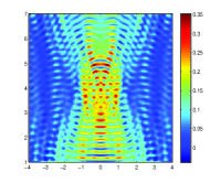
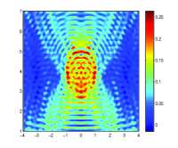
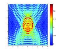
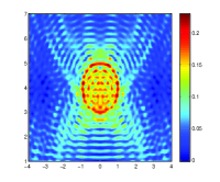
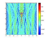
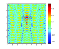
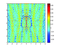
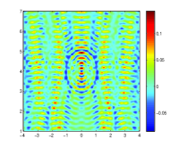
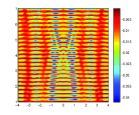
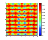
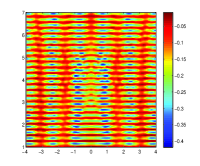
Fig. 3: The imaging results with the aperture $d=10,20,30,50$ from left to right, respectively. The top row shows the imaging results of our RTM algorithm (21). The middle and the bottom rows show the real and imaginary part of the Kirchhoff migration function (23).

The imaging results are shown in Figure 3. We observe that our RTM imaging function peaks at the boundary of the obstacle, while the imaging function $\tilde{I}_{d}(z)$ in (23) does not have this property. We remark that in [25] the Kirchhoff migration type imaging algorithm is successfully used in a setting different from ours: the sources and receivers in [25] span the full lateral direction of the waveguide which is perpendicular to the waveguide boundaries.

Example 2. In this example we first consider the imaging of a circle of radius $\rho=1$, a kite, and a rounded square with the impedance boundary condition with $\eta=1$ or $\eta=1000$ on $\Gamma_{D}$. Let $\Omega=(-4,4)\times(1,7)$ be the search region. The imaging function is computed at the nodal points of a uniform $201\times 201$ mesh with the probed wavelength $\lambda=0.5$. The imaging results on the top and bottom row shown in Figure 4 correspond to the surface impedance $\eta=1$ and $\eta=1000$, respectively. We observe our imaging algorithm is quite robust with respect to the magnitude of the surface impedance $\eta$.

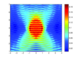
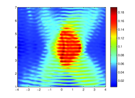
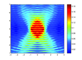
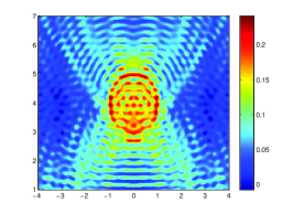
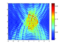
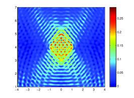
Fig. 4: The imaging results with the probe wavelength $\lambda=0.5$, the thickness $h=10$, the aperture $d=30$, and $N_{s}=N_{r}=401$ for a circle, a kite, and a rounded square, respectively, The top and bottom row show the imaging results of the RTM method for the surface impedance $\eta=1$ and $\eta=1000$, respectively.

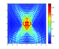
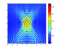
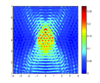
Fig. 5: The imaging results, from left to right, for the penetrable obstacle with $n(x)=0.25$, a non-penetrable obstacle with homogeneous Neumann condition, homogeneous Dirichlet condition, and partially coated impedance boundary condition ($\eta=1000$ on the upper half boundary and $\eta=1$ on the lower half boundary), respectively. The probe wavelength $\lambda=0.5$, the thickness $h=10$, the aperture $d=30$, and $N_{s}=N_{r}=401$.

We then consider to find a penetrable obstacle with the refraction index $n(x)=0.25$, a non-penetrable obstacle with homogeneous Neumann, homogeneous Dirichlet, and partially coated impedance boundary condition ($\eta=1000$ on the upper half boundary and $\eta=1$ on the lower half boundary), respectively. The results are shown in Figure 5 which indicates clearly that our RTM method can reconstruct the boundary of the obstacle without a priori information on penetrable or non-penetrable obstacles, and in the case of non-penetrable obstacles, the type of the boundary conditions on the boundary of the obstacle.

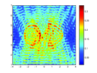
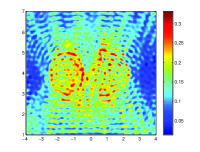
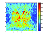
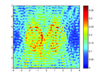
Fig. 6: The imaging results using data added with additive Gaussian noise and $\mu=10\%,20\%,30\%,40\%$ from left to right, respectively. The probe wavelength $\lambda=0.5$, the thickness $h=10$, the aperture $d=30$, and $N_{s}=N_{r}=401$.

Example 3. In this example we consider the stability of the imaging function with respect to the complex additive Gaussian random noise. We introduce the additive Gaussian noise as follows (see e.g. [10]):

$$u_{noise}=u_{s}+\nu_{\rm noise},$$

where $u_{s}$ is the synthesized data and $\nu_{\rm noise}$ is the complex Gaussian noise with mean zero and standard deviation $\mu$ times the maximum of the data $|u_{s}|$, i.e. $\nu_{\rm noise}=\frac{\mu\max|u_{s}|}{\sqrt{2}}(\varepsilon_{1}+\mathbf{i}\varepsilon_{2})$, and $\varepsilon_{j}~{}\thicksim\mathcal{N}(0,1)$ for the real $(j=1)$ and imaginary part $(j=2)$.

For the fixed probe wavelength $\lambda=0.5$, we choose one kite and one circle in our test. The search domain is $\Omega=(-4,4)\times(1,7)$ with a sampling $201\times 201$ mesh. Figure 6 shows the imaging results with the noise level $\mu=10\%,20\%,30\%,40\%$ in the single frequency scattered data, respectively. The left table in Table 1 shows the noise level in this case, where $\sigma=\mu\max_{x_{r},x_{s}}|u^{s}(x_{s},x_{r})|$, $\|u_{s}\|_{\ell^{2}}^{2}=\frac{1}{N_{s}N_{r}}\sum^{N_{s},N_{r}}_{s,r=1}|u^{s}(x_{s}.x_{r})|^{2}$, $\|\nu_{\rm noise}\|_{\ell^{2}}^{2}=\frac{1}{N_{s}N_{r}}\sum^{N_{s},N_{r}}_{s,r=1}|\nu_{\rm noise}(x_{s}.x_{r})|^{2}$.

The imaging quality can be improved by using multi-frequency data as illustrated in Figure 7, in which we show the imaging results added with the noise level $\mu=10\%,20\%,30\%,40\%$ Gaussian noise by summing the imaging functions for the probed wavelengths $\lambda=1/1.8,1/1.9,1/2.0,1/2.1,1/2.2$. The right table in Table 1 shows the noise level in the case of multi-frequency data, where $\sigma$, $\|u_{s}\|_{\ell^{2}}$, and $\|\nu_{\rm noise}\|_{\ell^{2}}$ are the arithmetic mean of the corresponding values for different frequencies, respectively. The imaging result is visually much more better than the single frequency imaging result, and the noise is greatly suppressed after the summation over individual frequency imaging results.

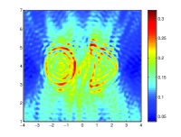
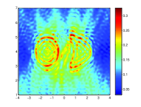
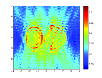
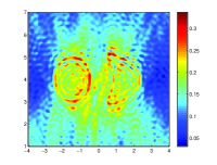
Fig. 7: The imaging results using multi-frequency data added with additive Gaussian noise and $\mu=10\%,20\%,30\%,40\%$ from left to right, respectively. The probe wavelengths $\lambda=1/1.8,1/1.9,1/2.0,1/2.1,1/2.2$, the thickness $h=10$, the aperture $d=30$, and $N_{s}=N_{r}=401$.

Table 1: The signal level and noise level in the case of single frequency data (left) and multi-frequency data (right).

$\mu$	$\sigma$	$\|u_{s}\|_{\ell^{2}}$	$\|\nu_{\rm noise}\|_{\ell^{2}}$
0.1	0.0360	0.1033	0.0293
0.2	0.0720	0.1033	0.0589
0.3	0.1079	0.1033	0.0876
0.4	0.1439	0.1033	0.1178

$\mu$	$\sigma$	$\|u_{s}\|_{\ell^{2}}$	$\|\nu_{\rm noise}\|_{\ell^{2}}$
0.1	0.0355	0.1033	0.0290
0.2	0.0710	0.1033	0.0580
0.3	0.1064	0.1033	0.0869
0.4	0.1419	0.1033	0.1159

8 Concluding remarks

In this paper we have developed a novel reverse time migration algorithm based on the generalized Helmholtz-Kirchhoff identity for the obstacle shape reconstruction in planar acoustic waveguide. The algorithm consists of using the half space Green function instead of the waveguide Green function in both the back-propagation and cross-correlation processes. The algorithm is quite robust with respect to the random noise. Our numerical experiments indicate that the RTM algorithm based on multiple frequency superposition can effectively suppress the random noise. Extending the results in this paper to the electromagnetic and elastic waveguide imaging problem is of considerable practical interests and will be pursued in our future works.

9 Appendix: Proof of Theorem 3

We will prove the existence of the radiation solution of the problem (11)-(13) by the method of limiting absorption principle. The argument is standard and generalizes that for Helmholtz scattering problem in the free space, see e.g. [18]. Here we only outline the main steps.

For any $z=1+\mathbf{i}\varepsilon$, $\varepsilon>0$, $f\in L^{2}({\mathbb{R}}^{2}_{h})$ with compact support in $B_{R}=(-R,R)\times(0,h)$, where $R>0$, we consider the problem

$$\Delta u_{z}+zk^{2}u_{z}=-f\qquad\mbox{in }{\mathbb{R}}^{2}_{h},$$ (62)

$$u_{z}=0\ \ \mbox{on }\Gamma_{0},\ \ \ \ \frac{\partial u_{z}}{\partial x_{2}}=0\ \ \mbox{on }\Gamma_{h}.$$ (63)

By Lax-Milgram lemma we know that (62)-(63) has a unique solution $u_{z}\in H^{1}({\mathbb{R}}^{2}_{h})$. For any domain $\mathcal{D}\subset{\mathbb{R}}^{2}_{h}$, we define the weighted space $L^{2,s}(\mathcal{D}),s\in{\mathbb{R}}$, by

$$L^{2,s}(\mathcal{D})=\{v\in L^{2}_{\rm loc}(\mathcal{D}):(1+|x_{1}|^{2})^{s/2}v\in L^{2}(\mathcal{D})\}$$

with the norm $\|v\|_{L^{2,s}(\mathcal{D})}=(\int_{\mathcal{D}}(1+|x_{1}|^{2})^{s}|v|^{2}dx)^{1/2}$. The weighted Sobolev space $H^{1,s}(\mathcal{D}),s\in{\mathbb{R}}$, is defined as the set of functions in $L^{2,s}(\mathcal{D})$ whose first derivative is also in $L^{2,s}(\mathcal{D})$. The norm $\|v\|_{H^{1,s}(\mathcal{D})}=(\|v\|^{2}_{L^{2,s}(\mathcal{D})}+\|\nabla v\|^{2}_{L^{2,s}(\mathcal{D})})^{1/2}$.

Lemma 16.

Let $f\in L^{2}({\mathbb{R}}^{2}_{h})$ with compact support in $B_{R}$. For any $z=1+\mathbf{i}\varepsilon$, $0<\varepsilon<1$, we have, for any $s>1/2$, $\|u_{z}\|_{H^{1,-s}({\mathbb{R}}^{2}_{h})}\leq C\|f\|_{L^{2}({\mathbb{R}}^{2}_{h})}$ for some constant independent of $\varepsilon,u_{z}$, and $f$.

Proof.

We first note that by testing (62) by $(1+|x_{1}|^{2})^{-s}\bar{u}_{z}$, $s>1/2$, one can obtain $\|u_{z}\|_{H^{1,-s}({\mathbb{R}}^{2}_{h})}\leq C\|u_{z}\|_{L^{2,s}({\mathbb{R}}^{2}_{h})}+C\|f\|_{L^{2}({\mathbb{R}}^{2}_{h})}$ by standard argument. It remains to show $\|u_{z}\|_{L^{2,s}({\mathbb{R}}^{2}_{h})}\leq C\|f\|_{L^{2}({\mathbb{R}}^{2}_{h})}$. It is obvious that we only need to prove the estimate for $f\in C^{\infty}_{0}({\mathbb{R}}^{2}_{h})$. We start with the following integral representation formula

$$u_{z}(x)=\int_{{\mathbb{R}}^{2}_{h}}N^{z}(x,y)f(y)dy,\ \ \ \ x\in{\mathbb{R}}^{2}_{h}.$$ (64)

Here $N^{z}(x,y)$ is the Green function of the problem (62)-(63) with the complex wave number $kz^{1/2}$, where $\mathrm{Im}\,(z^{1/2})>0$ for $\varepsilon>0$. Similar to (10), it is easy to check that

$$N^{z}(x,y)=\sum_{n=1}^{\infty}\frac{\textbf{i}}{h\xi^{z}_{n}}\sin(\mu_{n}x_{2})\sin(\mu_{n}y_{2})e^{\textbf{i}\xi^{z}_{n}|x_{1}-y_{1}|},$$ (65)

where $\xi^{z}_{n}=\sqrt{zk^{2}-\mu_{n}^{2}}$ whose imaginary part $\mathrm{Im}\,{\xi^{z}_{n}}\geq 0$. It follows from (64)-(65) that $u_{z}$ has the mode expansion

$$u_{z}(x)=\sum_{n=1}^{\infty}u_{n}^{z}(x_{1})\sin(\mu_{n}x_{2}),$$ (66)

where, since $f$ is supported in $B_{R}$,

$$u_{n}^{z}(x_{1})=\frac{h}{2}\int_{-R}^{R}\frac{\textbf{i}}{h\xi^{z}_{n}}e^{\textbf{i}\xi^{z}_{n}|x_{1}-y_{1}|}f_{n}(y_{1})dy_{1},\ \ \ \ f_{n}(x_{1})=\frac{2}{h}\int_{0}^{h}f(x)\sin(\mu_{n}x_{2})dx_{2}.$$

Since $\mathrm{Im}\,\xi^{z}_{n}\geq 0$ and $|\xi_{n}^{z}|^{2}=\sqrt{(\mu_{n}^{2}-k^{2})^{2}+(k^{2}\varepsilon)^{2}}\geq|\mu_{n}^{2}-k^{2}|$, we have

$$|u_{n}^{z}(x_{1})|\leq\frac{h}{2}\frac{\sqrt{2R}}{h|\mu_{n}^{2}-k^{2}|^{1/2}}\,\|f_{n}\|_{L^{2}({\mathbb{R}})}.$$

Therefore

$$\|u\|_{L^{2,-s}({\mathbb{R}}^{2}_{h})}^{2} = \frac{h}{2}\sum^{\infty}_{n=1}\int^{\infty}_{-\infty}(1+|x_{1}|^{2})^{-s}|u^{z}_{n}(x_{1})|^{2}dx_{1}$$

$$\leq \left(\frac{h}{2}\right)^{2}\|f\|^{2}_{L^{2}({\mathbb{R}}^{2}_{h})}\sum^{\infty}_{n=1}\int_{-\infty}^{+\infty}\frac{2R}{h^{2}|\mu^{2}_{n}-k^{2}|}(1+|x_{1}|^{2})^{-s}dx_{1}$$

$$\leq C\|f\|_{L^{2}({\mathbb{R}}^{2}_{h})}^{2}.$$

where we have used $\|f\|^{2}_{L^{2}({\mathbb{R}}^{2}_{h})}=\frac{h}{2}\sum^{\infty}_{n=1}\|f_{n}\|^{2}_{L^{2}({\mathbb{R}})}$. This completes the proof. ∎

Now we are ready to prove Theorem 3.

Proof of Theorem 3. For any $0<\varepsilon<1$, we consider the problem

$$\Delta u_{\varepsilon}+(1+\mathbf{i}\varepsilon)k^{2}u_{\varepsilon}=0\qquad\mbox{in }{\mathbb{R}}^{2}_{h}\backslash\bar{D},$$ (67)

$$u_{\varepsilon}=0\ \ \mbox{on }\Gamma_{0},\ \ \ \ \frac{\partial u_{\varepsilon}}{\partial x_{2}}=0\ \ \mbox{on }\Gamma_{h},{}$$ (68)

$$\frac{\partial u_{\varepsilon}}{\partial\nu}+\mathbf{i}k\eta u_{\varepsilon}=g\ \ \ \mbox{ on }\ \ \Gamma_{D}.{}$$ (69)

We know that the above problem has a unique solution $u_{\varepsilon}\in H^{1}({\mathbb{R}}^{2}_{h}\backslash\bar{D})$ by the Lax-Milgram Lemma.

Let $\chi\in C_{0}^{\infty}({\mathbb{R}}^{2}_{h})$ be the cut-off function such that $0\leq\chi\leq 1$, $\chi=0$ in $B_{R}$, and $\chi=1$ outside of $B_{R+1}$. Let $v_{\varepsilon}=\chi u_{\varepsilon}$, then $v_{\varepsilon}$ satisfies the equation (62) with $z=1+\mathbf{i}\varepsilon$ and $f=u_{\varepsilon}\Delta\chi+2\nabla u_{\varepsilon}\cdotp\nabla\chi$. Obviously, $f$ is supported in $B_{R+1}$. By Lemma 16, we have $\|v_{\varepsilon}\|_{H^{1,-s}({\mathbb{R}}^{2}_{h}\backslash\bar{D})}\leq C\|u_{\varepsilon}\|_{H^{1}(B_{R+1}\backslash\bar{D})}$. Since $\chi=1$ outside $B_{R+1}$, we have then

$$\|u_{\varepsilon}\|_{H^{1,-s}({\mathbb{R}}^{2}_{h}\backslash\bar{D})}\leq C\|u_{\varepsilon}\|_{H^{1}(B_{R+1}\backslash\bar{D})}.$$ (70)

Next let $\chi_{1}\in C_{0}^{\infty}({\mathbb{R}}^{2}_{h})$ be the cut-off function with that $0\leq\chi_{1}\leq 1$, $\chi_{1}=1$ in $B_{R+1}$, and $\chi_{1}=0$ outside of $B_{R+2}$. For $g\in H^{-1/2}(\Gamma_{D})$, let $u_{g}\in H^{1}({\mathbb{R}}^{2}_{h}\backslash\bar{D})$ be the lifting function such that $\frac{\partial u_{g}}{\partial\nu}+\mathbf{i}k\eta u_{g}=g\mbox{ on }\Gamma_{D}$ and $\|u_{g}\|_{H^{1}({\mathbb{R}}^{2}_{h}\backslash\bar{D})}\leq C\|g\|_{H^{-1/2}(\Gamma_{D})}$ hold. By testing (LABEL:wg2) with $\chi_{1}^{2}(\overline{u_{\varepsilon}-u_{g}})$, we have by the standard argument

$$\|u_{\varepsilon}\|_{H^{1}(B_{R+1}\backslash\bar{D})}\leq C(\|u_{\varepsilon}\|_{L^{2}(B_{R+2}\backslash\bar{D})}+\|g\|_{H^{-1/2}(\Gamma_{D})}).$$ (71)

Now we claim

$$\|u_{\varepsilon}\|_{L^{2}(B_{R+2}\backslash\bar{D})}\leq C\|g\|_{H^{-1/2}(\Gamma_{D})},$$ (72)

for any $g\in H^{-1/2}(\Gamma_{D})$ and $\varepsilon>0$. If it were false, there would exist sequences $\{g_{m}\}\subset H^{-1/2}(\Gamma_{D})$ and $\{\varepsilon_{m}\}\subset(0,1)$, and $\{u_{\varepsilon_{m}}\}$ be the corresponding solution of (LABEL:wg2)-(69) such that

$${}\|u_{\varepsilon_{m}}\|_{L^{2}(B_{R+2}\backslash\bar{D})}=1\ {\rm{and}}\ \|g_{m}\|_{H^{-1/2}(\Gamma_{D})}\leq\frac{1}{m}.$$ (73)

Then $\|u_{\varepsilon_{m}}\|_{H^{1,-s}({\mathbb{R}}^{2}_{h}\backslash\bar{D})}\leq C$, and thus there is a subsequence of $\{\varepsilon_{m}\}$, which is still denoted by $\{\varepsilon_{m}\}$, such that $\varepsilon_{m}\to\varepsilon^{\prime}\in[0,1]$, and a subsequence of $\{u_{\varepsilon_{m}}\}$, which is still denoted by $\{u_{\varepsilon_{m}}\}$, such that it converges weakly to some $u_{\varepsilon^{\prime}}\in H^{1,-s}({\mathbb{R}}^{2}_{h}\backslash\bar{D})$. The function $u_{\varepsilon^{\prime}}$ satisfies (LABEL:wg2)-(69) with $g=0$ and $\varepsilon=\varepsilon^{\prime}$ . By the integral representation formula, we have, for $x\in{\mathbb{R}}^{2}_{h}\backslash\bar{D}$,

$$u_{\varepsilon^{\prime}}(x)=-\int_{\Gamma_{D}}\left(\frac{\partial N^{1+\mathbf{i}\varepsilon^{\prime}}(x,y)}{\partial\nu(y)}u_{\varepsilon^{\prime}}(y)-N^{1+\mathbf{i}\varepsilon^{\prime}}(x,y)\frac{\partial u_{\varepsilon^{\prime}}(y)}{\partial\nu(y)}\right)ds(y).$$ (74)

If $\varepsilon^{\prime}>0$, we deduce from (74) that $u_{\varepsilon^{\prime}}$ decays exponentially and thus $u_{\varepsilon^{\prime}}\in H^{1}({\mathbb{R}}^{2}_{h}\backslash\bar{D})$, then $u_{\varepsilon^{\prime}}=0$ by the uniqueness of the solution in $H^{1}({\mathbb{R}}^{2}_{h}\backslash\bar{D})$ with positive absorption. If $\varepsilon^{\prime}=0$, (74) implies that $u_{\varepsilon^{\prime}}$ satisfies the mode radiation condition (7), and then $u_{\varepsilon^{\prime}}=0$ by the uniqueness Lemma 2. Therefore, in any case, $u_{\varepsilon^{\prime}}=0$, which, however, contradicts to (73).

This shows (72). Consequently, by (70) and (71),

$$\|u_{\varepsilon}\|_{H^{1,-s}({\mathbb{R}}^{2}_{h}\backslash\bar{D})}\leq C\|g\|_{H^{-1/2}(\Gamma_{D})}.$$ (75)

Now, it is easy to see that $u_{\varepsilon}$ has a convergent subsequence which converges weakly to some $u\in H^{1,-s}({\mathbb{R}}^{2}_{h}\backslash\bar{D})$ and satisfies (11)-(13). The desired estimate follows from (75). This completes the proof.   $\Box$

Acknowledgement. We would like to thank the referees for their insightful comments which lead to great improvement of the paper.

References

[1]H. Ammari, E. Iakovleva, and H. Kang, Reconstruction of a small inclusion in a 2D open waveguide, SIAM J. Appl. Math., 65 (2005), pp. 2107-2127.
[2]T. Arens, D. Gintides, and A. Lechleiter, Variational formulations for scattering in a
3-dimensional acoustic waveguide, Math. Meth. Appl. Sci., 31 (2008), pp. 82-847.
[3]T. Arens, D. Gintides, and A. Lechleiter, Direct and inverse medium scattering in a three-dimensional homogeneous planar waveguide,
SIAM J. Appl. Math., 71 (2011), pp. 753-772.
[4]A.J. Berkhout, Seismic Migration: Imaging of Acoustic Energy by Wave Field Extrapolation, Elsevier, New York, 1984.
[5]N. Bleistein, J. Cohen, and J. Stockwell, Mathematics of Multidimensional Seismic Imaging, Migration, and Inversion, Springer, New York, 2001.
[6]L. Bourgeois and E. Luneville, The linear sampling method in a waveguide: a modal formulation, Inverse Problems, 24 (2008), pp. 1-20.
[7]L. Borcea, L. Issa, and C. Tsogka, Source localization in random acoustic waveguide, Multiscale Model. Simul., 8 (2010), pp. 1981-2022.
[8]L.D. Carli, S. Hudson, and X. Li, Minimum potential results for the Schrödingier equation in a slab, Preprint, 2013.
[9]S.N. Chandler-Wilde, I.G. Graham, S. Langdon, and M. Lindner, Condition number estimates for combined
potential boundary integral operators in acoustic scattering, J. Integral Equations Appl., 21 (2009), pp. 229-279.
[10]J. Chen, Z. Chen, and G. Huang, Reverse time migration for extended obstacles: acoustic waves, Inverse Problem, 29 (2013), 085005 (17pp).
[11]J. Chen, Z. Chen, and G. Huang, Reverse time migration for extended obstacles: electromagnetic waves, Inverse Problem, 29 (2013), 085006 (17pp).
[12]W.C. Chew, Waves and Fields in Inhomogeneous Media, Van Nodtrand Reimhold, New York, 1990.
[14]D. Colton and R. Kress, Inverse Acoustic and Electromagnetic Scattering Problems, Springer, Heidelberg, 1998.
[15]L. Grafakos,Classical and Modern Fourier Analysis, Pearson, London, 2004.
[16]K. Ito, B. Jin, and J. Zou, A direct sampling method to an inverse medium scattering problem, Inverse Problem, 28 (2012), 025003 (11pp).
[17]S. Kim, G. Edelmann, W. Kuperman, W. Hodgkiss, and H. Song,
Spatial resolution of time-reversal arrays in shallow water, J. Acoust. Soc. Am., 110 (2001), pp. 820-829.
[18]R. Leis, Initial Boundary Value Problems in Mathematical Physics, B.G. Teubner, Stuttgart, 1986.
[19]C.M. Linton and P. McIver, Embedded trapped modes in water waves and acoustics, Wave Motion, 45 (2007), pp. 16-29.
[20]K. Morgenrother and P. Werner, Resonances and standing waves, Math. Meth. Appl. Sci., 9 (1987), pp. 105-126.
[21]K. Morgenrother and P. Werner, On the principles of limiting absorption and limiting amplitude
for a class of locally perturbed waveguides, Math. Meth. Appl. Sci., 10 (1988), pp. 125-144.
[22]A. Ramm and G. Makrakis, Scattering by obstacles in acoustic waveguides, In Spectral
and Scattering Theory (Ramm A G ed.), Plenum publishers (1998), pp. 89-110.
[23]C. Roziery, D. Lesseliery, T. Angell, and R. Kleinman,
Shape retrieval of an obstacle immersed in shallow water from single-frequency farfields using a complete family
method, Inverse Problems, 13 (1997), pp. 487-508.
[24]J. Sun and C. Zheng, Reconstruction of obstacles embedded in waveguides, Contemporary Mathematics, 586 (2013), pp. 341-350.
[25]C. Tsogka, D.A. Mitsoudis, and S. Papadimitropoulos, Selective imaging of extended relectors in two-dimensional waveguides,
SIAM J. Imaging Sci., 6 (2013), pp. 2714-2739.
[26]W.L. Voxman, Advanced Calculus: An Introduction to Modern Analysis, Marcel Dekker, Inc., New York, 1981.
[27]Y. Xu, The propagation solutions and far-field patterns for acoustic harmonic waves in a finite
depth ocean, Appl. Anal., 35 (1990), pp. 129-151.
[28]Y. Xu, C. Mawata, and W. Lin, Generalized dual space indicator method for underwater
imaging, Inverse Problems, 16 (2000), pp. 176-1776.
[29]G.N. Watson, A Treatise on the Theory of Bessel Functions, Cambridge University Press, Cambridge, 1922.