Existence of nonlinear normal modes for coupled nonlinear oscillators

Abstract

We prove the existence of nonlinear normal modes for general systems of two coupled nonlinear oscillators. Facilitating the comparison principle for ordinary differential equations it is shown that there exist exact solutions representing a vibration in unison of the system. The associated spatially localised time-periodic solutions feature out-of-phase and in-phase motion of the oscillators.

1 Introduction

The concept of normal modes plays a central role for the theory of oscillations of linear system. In a normal mode the dynamics of a finite linear system is equivalent to those of a system with one degree of freedom. Linear normal modes (LNMs) can be used to decouple a linear system of $n$ degrees of freedom of coupled oscillators such that it performs oscillatory motions resulting from the superposition of its eigensolutions with associated eigenfrequencies. The repercussions are: (i) That if a specific eigenmode only is stimulated then the motion is restrained to the corresponding harmonic oscillations and energy transfer into other modes is impossible (invariance). (ii) Any form of free or harmonically forced oscillatory motion can be expressed as the superposition of the $n$ modes of natural frequencies. These modes result in stationary periodic solutions for which all units pass through their extreme values of the coordinates and velocities simultaneously (modal superposition).

However, the assumption of linearity seems too idealised as it is justifiable typically for sufficiently small amplitudes only. Thus in general one deals inevitably with nonlinear restoring forces for which the linear methods such as the superposition principle is not applicable.

To gain insight into the response of a nonlinear system to excitations elaborate methods based on perturbational approaches to derive (approximate) solutions have been developed which rely on weak nonlinearity perturbation . On the other hand, for large amplitude dynamics related to strong nonlinearity the expression of exact solutions of the underlying system of ordinary differential equations in closed analytical form (if existent at all) is in most cases impossible. Regarding exact solutions of finite nonlinear systems the concept of nonlinear normal modes (NNMs) was developed to understand dynamical features of systems featuring strong nonlinearity. Like their linear counterparts NNMs are understood as a vibration in unison of the system, i.e. all units of the system perform synchronous oscillations Rosenberg . Compared to their linear counterpart for NNMs the superposition principle does not apply and the lack of orthogonality relations restricts their usage as bases for the expression of solutions of the underlying nonlinear system in terms of weighted sums of eigenfunctions. A generalised definition of NNMs by geometric means utilising the center manifold technique was given by Shaw and Pierre Shaw . The existence of NNMs of Hamiltonian systems obeying certain symmetries has been addressed in existence1 -existence2 .

The role of NNMs with regard to the qualitative and quantitative investigation of nonlinear features has been illuminated in numerous studies (see e.g. Rand -Belizzi and for a recent review we refer to Avramov and references therein). To underline the significance of NNMs for the interpretation of nonlinear phenomena, the driven resonant motion of nonlinear systems evolves close to NNMs and localisation and energy transfer can be explained in terms of NNMs existence2 . Recently the concept of NNMs has been facilitated as a theoretical tool to accomplish targeted energy transfer Kopidakis -targeted . Studies of NNMs in non-smooth systems have been performed in Jiang ,Vestroni .

The aim of the current paper is to prove the existence of NNMs for a general system of two coupled oscillators represented by spatially localised and time-periodic solutions. We treat two types of on-site potentials; namely hard and soft ones. Unlike for the continuation process of (trivially) localised solutions starting from the anti-continuum limit Marin -Martinez2 our approach is not necessarily confined to the weak coupling regime.

2 The system of two coupled general oscillators

In this work we prove the existence of spatially localised time-periodic solutions, i.e. NNMs, for generic nonlinear interacting oscillators given by the following system

$$\ddot{q}_{1}(t) = -U^{\prime}(q_{1}(t))-\kappa V^{\prime}(q_{12}(t)),$$ (1)

$$\ddot{q}_{2}(t) = -U^{\prime}(q_{2}(t))+\kappa V^{\prime}(q_{12}(t)).$$ (2)

The variable $q_{n}(t)$ is the amplitude of the oscillator at site $n$ evolving in an anharmonic on-site potential $U(q_{n})$. We introduced the notation $q_{12}=q_{1}-q_{2}$. The prime ^′ stands for the derivative with respect to the argument and an overdot $\dot{}$ represents the derivative with respect to time $t\in{\mathbb{R}}$. The two oscillators interact with each other via an attractive force derived from an interaction potential $V(u)$ which is analytic and furthermore, is assumed to have the following features:

$$V(0)=V^{\prime}(0)=0,\,\,\,V^{\prime\prime}(0)\geq 0,\,\,\,V^{\prime\prime}(u\neq 0)>0.$$ (3)

Thus $V(u)$ is convex which is further characterised by $V^{\prime}(u>0)>0$ and $V^{\prime}(u<0)<0$. The interaction potential can be harmonic (diffusive interaction) but also anharmonic such as e.g. interactions of $\beta-$Fermi-Pasta-Ulam-type and Toda-type. The strength of the coupling is determined by the value of $\kappa$.

The on-site potential $U$ is analytic and is assumed to have the following properties:

$$U(0)=U^{\prime}(0)=0\,,\,\,\,U^{\prime\prime}(0)>0.$$ (4)

In what follows we differentiate between soft on-site potentials and hard on-site potentials. For the former (latter) the oscillation frequency of an oscillator moving in the on-site potential $U(q)$ decreases (increases) with increasing oscillation amplitude. A soft potential possesses at least one inflection point. If a soft potential possesses a single inflection point, denoted by $q_{i}$, we suppose without loss of generality (w.l.o.g.) that $q_{i}>0$. Then the following relations are valid

$$U^{\prime}(-\infty<q<0) < 0,\,\,\,U^{\prime}(0<q<q_{i})>0,$$ (5)

$$U^{\prime\prime}(q_{i}) = 0,\,\,\,U^{\prime\prime}(-\infty<q<q_{i})>0.$$ (6)

If $U(q)$ possesses two inflection points denoted by $q_{i,-}<0$ and $q_{i,+}>0$ it holds that

$$U^{\prime}(q_{i,-}<q<0) < 0,\,\,\,U^{\prime}(0<q<q_{i,+})>0$$ (7)

$$U^{\prime\prime}(q_{i,\pm}) = 0,\,\,\,U^{\prime\prime}(q_{i,-}<q<q_{i,+})>0.$$ (8)

We remark that $U(q)$ can have more than two inflection points (an example is a periodic potential $U(q)=-\cos(q)$). However, in the frame of the current study we are only interested in motion between the inflection points adjacent to the minimum of $U(q)$ at $q=0$. Hence, in the forthcoming we make the assumption that for soft on-site potentials the motion at each lattice site $n=1,2$ stays inbetween the inflection points, viz. $q_{i,-}<q_{l}\leq q_{n}(t)\leq q_{r}<q_{i,+}$, where $U(q)$ is convex.

Hard on-site potentials are, in addition to the assumptions in (4), characterised in their entire range of definition by

$$U^{\prime}(q<0)<0,\,\,\,U^{\prime}(q>0)>0,\,\,\,U^{\prime\prime}(q)>0.$$ (9)

For hard on-site potentials we make the assumption that the motion takes place in the range $q_{1,2}(t)\in[Q_{l},Q_{r}]$, with $-\infty<Q_{l}<0$ and $0<Q_{r}<\infty$ for $t>0$.

The system (1),(2) possesses an energy integral

$$E=\sum_{n=1}^{2}\left[\frac{1}{2}\dot{q}_{n}^{2}+U(q_{n})\right]+\kappa V(q_{1}-q_{2}).$$ (10)

There exists a closed maximum equipotential surface $U(q_{1})+U(q_{2})+\kappa V(q_{1}-q_{2})=E$ bounding all motions and one has $\dot{q}_{1}=\dot{q}_{2}=0$ on this surface.

3 NNMs for coupled nonlinear oscillators in soft on-site potentials

In the following we prove the existence of NNMs for the system (1),(2) with soft on-site potentials. In more detail, we show that there exists a one-parameter family of spatially localised and time-periodic solutions where the amplitude acts as the parameter. Localisation means that either $|q_{1}(t)|\geq|q_{2}(t)|$ or $|q_{1}(t)|\leq|q_{2}(t)|$ for all $t$, and equality holds only at moments of time when the amplitudes of two oscillators pass simultaneously through zero. The goal is to prove that such localised periodic solutions exist under general conditions on $U$ and $V$. We emphasise that the existence of localised solutions has to be distinguished from the fact that simply due to exchange symmetry, $q_{1}\leftrightarrow q_{2}$, of the underlying system an in-phase mode with equal amplitudes $q_{1}(t)=q_{2}(t)$ always exists. Furthermore, if, in addition, the potential $U(q)$ possesses the spatial reflexion symmetry $U(q)=U(-q)$, an out-of-phase mode characterised by $q_{1}(t)=-q_{2}(t)$ is supported.

Theorem 1: Let $(q_{n}(t),\dot{q}_{n}(t))$ be the smooth solutions to Eqs. (1),(2) with a soft on-site potential satisfying the assumptions above. Then there exist periodic solutions $(q_{n}(t+T_{b}),\dot{q}_{n}(t+T_{b}))=(q_{n}(t),\dot{q}_{n}(t))$ for $n=1,2$, so that the oscillators perform either in-phase motion, i.e. $\operatorname{sign}(q_{1}(t))=\operatorname{sign}(q_{2}(t))$, or out-of-phase motion, i.e. $\operatorname{sign}(q_{1}(t))=-\operatorname{sign}(q_{2}(t))$, with period $T_{b}=2\pi/\omega_{b}$ and frequency $\omega_{b}$ satisfying

$$\sqrt{\min\{U^{\prime\prime}(q_{l}),U^{\prime\prime}(q_{r})\}}\leq\omega_{b}<\sqrt{U^{\prime\prime}(0)+2\tilde{\kappa}}$$ (11)

where $\tilde{\kappa}=\max\{V^{\prime\prime}(q_{l}),V^{\prime\prime}(q_{r})\}\kappa$.

Moreover, the solutions are localised which is characterised by either

$$|q_{1}(t)|\geq|q_{2}(t)|,\,\,\,t\in{\mathbb{R}}$$ (12)

or

$$|q_{2}(t)|\geq|q_{1}(t)|,\,\,\,t\in{\mathbb{R}}.$$ (13)

Proof: W.l.o.g. the initial conditions satisfy

$$q_{1}(0)=q_{2}(0)=0,\,\,\,|\dot{q}_{2}(0)|<|\dot{q}_{1}(0)|.$$ (14)

First, we consider initial conditions $q_{1}(0)=q_{2}(0)=0$ and in-phase initial velocities $0<\dot{q}_{2}(0)<\dot{q}_{1}(0)$ and show the existence of localised periodic in-phase solutions.

Then due to continuity there must exist some $t_{*}>0$ so that during the interval $[0,t_{*}]$ the following order relation is satisfied

$$q_{2}(t)\leq q_{1}(t).$$ (15)

We define the difference variable between the coordinates at sites $n=1$ and $n=2$ as follows

$$\Delta q_{*}(t)=q_{1}(t)-q_{2}(t).$$ (16)

Thus by definition $\Delta q_{*}(t)\geq 0$ on $[0,t_{*}]$.

The time evolution of the difference variables $\Delta q_{*}(t)$ is determined by the following equation

$$\frac{d^{2}\Delta q_{*}}{dt^{2}}=-\left[U^{\prime}(q_{1})-U^{\prime}(q_{2})\right]-2\kappa\frac{\partial V(q_{1}-q_{2})}{\partial q_{1}},$$ (17)

where we used that ${\partial V(q_{1}-q_{2})}/{\partial q_{2}}=-{\partial V(q_{1}-q_{2})}/{\partial q_{1}}$.

Discarding the negative term $-2{\kappa}{\partial V(q_{1}-q_{2})}/{\partial q_{1}}<0$ and utilising that for $q_{1}(t)\geq q_{2}(t)$

$$U^{\prime\prime}(0)(q_{1}-q_{2})\geq U^{\prime}(q_{1})-U^{\prime}(q_{2})\geq\Omega^{2}_{s}(q_{1}-q_{2})>0.$$ (18)

with $\Omega^{2}_{s}=\min\{U^{\prime\prime}(q_{l}),U^{\prime\prime}(q_{r})\}$ AIP enables us to bound the r.h.s. of Eq. (17) from above as follows:

$$\frac{d^{2}\Delta q_{*}}{dt^{2}}\leq-\Omega^{2}_{s}\Delta q_{*}(t).$$ (19)

Using the properties of the interaction potential (cf. Eqs. (3)) one gets $-\max\{V^{\prime\prime}(q_{l}),V^{\prime\prime}(q_{r})\}u\leq-V^{\prime}(u)$ for $u\geq 0$, so that we bound the r.h.s. of Eq. (17) for $q_{1}(t)\geq q_{2}(t)$ from below as follows:

$$\frac{d^{2}\Delta q_{*}}{dt^{2}}\geq-(\omega^{2}_{0}+2{\tilde{\kappa}})\Delta q_{*}(t),$$ (20)

with $\omega^{2}_{0}=U^{\prime\prime}(0)$.

Therefore, by the comparison principle for differential equations, $\Delta q_{*}(t)$ and $\Delta\dot{q}_{*}(t)$ are bounded from above and below for given initial conditions by the solution of

$$\frac{d^{2}a}{dt^{2}}=-\Omega^{2}_{s}a$$ (21)

and

$$\frac{d^{2}b}{dt^{2}}=-(\omega^{2}_{0}+2{\tilde{\kappa}})b,$$ (22)

respectively, provided $a(t)\geq 0$ and $b(t)\geq 0$.

The solution to Eq. (21) and (22) with initial conditions $(\Delta q_{*}(0)=0,\Delta\dot{q}_{*}(0^{+})\equiv\Delta\dot{q}_{0}\neq 0)$ is given by

$$a(t) = \frac{\Delta\dot{q}_{0}}{\Omega_{s}}\sin(\Omega_{s}t),$$ (23)

$$\dot{a}(t) = \Delta\dot{q}_{0}\cos(\Omega_{s}t)$$ (24)

and

$$b(t) = \frac{\Delta\dot{q}_{0}}{\sqrt{\omega^{2}_{0}+2{\tilde{\kappa}}}}\sin(\sqrt{\omega^{2}_{0}+2{\tilde{\kappa}}}\,t),$$ (25)

$$\dot{b}(t) = \Delta\dot{q}_{0}\cos(\sqrt{\omega^{2}_{0}+2{\tilde{\kappa}}}\,t),$$ (26)

respectively where $a(t)\geq 0$ for $0\leq t\leq\pi/\Omega_{s}$ and $b(t)\geq 0$ for $0\leq t\leq\pi/\sqrt{\omega^{2}_{0}+2{\tilde{\kappa}}}$. By $f(\tau_{k}^{-})$ and $f(\tau_{k}^{+})$ the left-sided and right-sided limits of $f(t)$ for $t\rightarrow\tau_{k}$ are meant, respectively.

Notice that $d^{2}\Delta q_{*}(t)/dt^{2}\leq 0$ on $(0,t_{*})$, that is, the acceleration stays non-positive. Due to the relations $\Delta\dot{q}_{0}>0$ in conjunction with the lower bound $b(t)\leq\Delta q_{*}(t)$ the order relation as given in (15) is at least maintained on the interval $[0,\pi/\sqrt{\omega^{2}_{0}+2{\tilde{\kappa}}}]$. Moreover, $\Delta q_{*}(t)$ is bound to grow monotonically at least during the interval $(0,\pi/(2\sqrt{\omega^{2}_{0}+2{\tilde{\kappa}}})]$ and attains a least maximal value $\Delta\dot{q}_{0}/\sqrt{\omega^{2}_{0}+2{\tilde{\kappa}}}$. Furthermore, $\Delta q_{*}(t)$ cannot return to zero before $t=\pi/\sqrt{\omega^{2}_{0}+2{\tilde{\kappa}}}$.

From the upper bound $\Delta q_{*}(t)\leq a(t)$ one infers that $\Delta q_{*}(t)$ can attain an absolute maximal value $\Delta\dot{q}_{0}/\Omega_{s}$ but not before $t=\pi/(2\Omega_{s})$ and $\Delta q_{*}(t)$ is bound to return to zero not later than $t=\pi/\Omega_{s}$. Similarly, $\Delta\dot{q}_{*}(t)$ is bound to decrease monotonically for $0<t\leq\pi/\Omega_{s}$ and becomes negative at a time in the interval
$(\pi/(2\sqrt{\omega^{2}_{0}+2{\tilde{\kappa}}}),\pi/(2\Omega_{s}))$. Moreover, it holds that
$\Delta\dot{q}_{*}(t)\geq-\Delta\dot{q}_{0}$ for $0\leq t\leq\pi/\sqrt{\omega^{2}_{0}+2{\tilde{\kappa}}}$ and $\Delta\dot{q}_{*}(t)\leq-\Delta\dot{q}_{0}$ for $t\geq\pi/\Omega_{s}$.

Therefore, by the smooth dependence of the solutions $(\Delta q(t),\Delta\dot{q}(t))$ on the initial values $(q_{1,2}(0),\dot{q}_{1,2}(0))$, to any chosen initial condition $q_{1}(0)=0,\dot{q}_{1}(0)\neq 0$ and $q_{2}(0)=0$ there exists a corresponding $\dot{q}_{2}(0)$ (or vice versa) so that one has $\Delta q_{*}(t_{*})=\Delta q_{*}(0)=0$ and $\Delta\dot{q}_{*}(t_{*}^{-})=-\Delta\dot{q}_{0}$ with $t_{*}\in[\pi/\sqrt{\omega^{2}_{0}+2{\tilde{\kappa}}},\pi/\Omega_{s}]$. This implies the symmetry

$$\Delta q_{*}(t_{*}/2+\tau) = \Delta q_{*}(t_{*}/2-\tau),$$ (27)

$$-\Delta\dot{q}_{*}(t_{*}/2+\tau)) = \Delta\dot{q}_{*}(t_{*}/2-\tau))$$ (28)

with $0<\tau<t_{*}/2$ and $t_{*}/2$ corresponds to the turning point of the motion when $\Delta q_{*}$ attain its maximum while $\Delta\dot{q}_{*}$ is zero. In turn, this implies that the motion of the two oscillators possesses the symmetry

$$\ q_{n}(t_{*}/2+\tau) = q_{n}(t_{*}/2-\tau),\,\,\,n=1,2$$ (29)

$$\dot{q}_{n}(t_{*}/2+\tau) = \dot{q}_{n}(t_{*}/2-\tau)),\,\,\,n=1,2,$$ (30)

with $0\leq\tau\leq t_{*}/2$ and $t_{*}/2$ corresponds to the turning point of the motion when $q_{1}$ and $q_{2}$ assume simultaneously their respective maxima while $\dot{q}_{1}$ and $\dot{q}_{2}$ pass simultaneously through zero. Conclusively, on the interval $[0,t_{*}]$ the two oscillators evolve through half a cycle of periodic in-phase motion, i.e. $\operatorname{sign}(q_{1})=\operatorname{sign}(q_{2})$ and $\operatorname{sign}(\dot{q}_{1})=\operatorname{sign}(\dot{q}_{2})$.

At $t=t_{*}$, just as at $t=0$, the oscillators pass simultaneously through zero coordinate, corresponding to the minimum position of the on-site potential at $q_{n}=0$ and the oscillators proceed afterwards with negative amplitude, i.e. $q_{n}(t)<0$ and negative velocity, i.e. $\dot{q}_{n}(t)<0$, $n=1,2$, until the next turning point is reached.

Since $\dot{q}_{1}(t_{*})<\dot{q}_{2}(t_{*})<0$ then due to continuity there must exist some $t_{**}>0$ so that during the interval $[t_{*},t_{**}]$ the following order relation is satisfied

$$q_{1}(t)\leq q_{2}(t).$$ (31)

For $t\geq t_{*}$ we consider the difference variable between the coordinates at sites $n=1$ and $n=2$ as follows

$$\Delta q_{**}(t)=q_{2}(t)-q_{1}(t).$$ (32)

Initialising the dynamics accordingly with $\Delta q_{**}(t_{*})=\Delta q_{*}=0$, $\Delta\dot{q}_{**}(t_{*}^{+})=\Delta\dot{q}_{*}(0^{+})$ and with the arguments given above it follows that $\Delta q_{**}(t)$ and $\Delta\dot{q}_{**}(t)$ exhibit qualitatively the same features as $\Delta q_{*}(t)$ and $\Delta\dot{q}_{*}(t)$ for $0\leq t\leq t_{*}$ and lower and upper bounds on $\Delta q_{**}(t)$ and $\Delta\dot{q}_{**}(t)$ are derived equivalently to the ones above. In fact, one has

$$q_{n}((t_{*}+t_{**})/2+\tau) = q_{n}((t_{*}+t_{**})/2-\tau),$$ (33)

$$\dot{q}_{n}((t_{*}+t_{**})/2+\tau) = \dot{q}_{n}((t_{*}+t_{**})/2-\tau),$$ (34)

with $n=1,2$ and $0\leq\tau\leq(t_{**}-t_{*})/2$ and $(t_{*}+t_{**})/2$ corresponds to the turning point of the motion when $q_{1,2}$ attain their minima while $\dot{q}_{1,2}$ pass through zero.

In particular the time $t_{**}$ at which $\Delta q_{**}(t_{**})=0$ and $\Delta\dot{q}_{**}(t_{**}^{-})=-\Delta\dot{q}_{**}(t_{*}^{+})$ lies in the range $t_{*}+\pi/\sqrt{\omega^{2}_{0}+2\tilde{\kappa}}<t_{**}<t_{*}+\pi/\Omega_{s}$. The zero of $\Delta q_{**}$ marks the end of a (first) cycle of duration $2\pi/\sqrt{\omega^{2}_{0}+2\tilde{\kappa}}<T_{b}=t_{**}<2\pi/\Omega_{s}$ of maintained localised oscillation throughout of which the order relation $|q_{1}(t)|\geq|q_{2}(t)|$ is preserved.

Notice that $t_{*}$ does not necessarily equals $t_{**}-t_{*}$ when the oscillators perform motion in on-site potentials without reflection symmetry, viz. $U(q)\neq U(-q)$. We remark that the frequency $\omega_{b}=2\pi/T_{b}$ depends on the amplitude $\bar{q}=\max\{q_{l},q_{r}\}$ and the latter can be chosen such that the non-resonance condition $m\omega_{b}(\bar{q})\neq\omega_{0}$ for all $m\in\mathbb{Z}$ is satisfied.

In relation to the time-periodicity of the dynamics of localised solutions (NNMs) beyond times $t\geq t_{**}$ we consider intervals

$$I_{k}:=[t_{k},t_{k+1}],\,\,\,\mbox{with integer}\,\,\,k\geq 1,\,\,\,t_{1}=t_{**}$$ (35)

with

$$t_{k+1}=\left\{\begin{array}[]{cl}t_{k}+t_{*}&\mbox{for}\,\,\,k\,\,\,\mbox{odd}\\ t_{k}+t_{**}-t_{*}&\mbox{for}\,\,\,k\,\,\,\mbox{even}\,.\\ \end{array}\right.$$ (36)

Crucially, on each of the intervals $I_{k}$, $q_{n}(t)$ and $\dot{q}_{n}(t)$, $n=1,2$, periodically repeat the behaviour of maintained localised oscillations, described above for the interval $[0,t_{*}]$ for odd $k$ and, $[t_{*},t_{**}]$ for even $k$. Conclusively, spatially localised and time-periodic solutions (NNMs) result satisfying

$$|q_{1}(t)|\geq|q_{2}(t)|,$$ (37)

and $(q_{n}(t+T_{b}),\dot{q}_{n}(t+T_{b}))=(q_{n}(t),\dot{q}_{n}(t))$ for $n=1,2$ with period $T_{b}=2\pi/\omega_{b}$ where the frequency $\omega_{b}$ satisfies the relations

$$\sqrt{\min\{U^{\prime\prime}(q_{l}),U^{\prime\prime}(q_{r})\}}\leq\omega_{b}<\sqrt{U^{\prime\prime}(0)+2\tilde{\kappa}},$$ (38)

and the out-of-phase NNM is of higher frequency than its in-phase counterpart.

The solutions possess the symmetries

$$q_{n}((t_{*}+(2l+1)t_{**})/2+t) = q_{n}((t_{*}+(2l+1)t_{**})/2-t),$$

$$-\dot{q}_{n}((t_{*}+(2l+1)t_{**})/2+t) = \dot{q}_{n}((t_{*}+(2l+1)t_{**})/2-t),$$

and

$$q_{n}((t_{*}+lt_{**})/2+t) = q_{n}((t_{*}+lt_{**})/2-t),$$

$$-\dot{q}_{n}((t_{*}+lt_{**})/2+t) = \dot{q}_{n}((t_{*}+lt_{**})/2-t),.$$

with $n=1,2$, $l\in{\mathbb{Z}}$ and initialising the dynamics with

$$q_{1,2}(0)=q_{1,2}((t_{*}+(2l+1)t_{**})/2),\dot{q}_{1,2}(0)=0,$$

or

$$q_{1,2}(0)=q_{1,2}((t_{*}+lt_{**})/2),\dot{q}_{1,2}(0)=0$$

yields time-reversible solutions, viz. $q_{1,2}(t)=q_{1,2}(-t)$ and $-\dot{q}_{1,2}(t)=\dot{q}_{1,2}(-t)$.

Consequently, the relation (37) is true for $t\in{\mathbb{R}}$. We remark that the case of out-of-phase initial velocities, $\operatorname{sign}(\dot{q}_{1}(0))=-\operatorname{sign}(\dot{q}_{2}(0))$, is treated in the same way as above and the proof is complete.

$\square$

For an illustration we show in Fig. 1 the periodic in-phase oscillations of the coordinates $q_{1}$ and $q_{2}$ for motion in a soft on-site potential given by

$$U(q)=\frac{1}{2}q^{2}-\frac{1}{4}q^{4},$$ (39)

and linear coupling originating from the harmonic interaction potential

$$V(q_{1}-q_{2})=\frac{\kappa}{2}(q_{1}-q_{2})^{2}.$$ (40)

The localisation feature of the NNM is reflected in $|q_{1}(t)|\geq|q_{2}(t)|$.

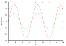
Figure 1: Periodic oscillations of the two coordinates $q_{1}$ and $q_{2}$ with $|q_{1}(t)|\geq|q_{2}(t)|$, corresponding to an in-phase NNM for motion in the soft on-site potential given in (39) and harmonic coupling of strength $\kappa=0.1$. The initial conditions are given by $q_{1}(0)=q_{2}(0)=0$ and $p_{1}(0)=0.5$, $p_{2}(0)=0.23$.

4 NNMs for motions in hard on-site potentials

In this section we consider hard on-site potentials. The next Theorem establishes the existence of NNMs represented by spatially localised and time-periodic solutions in hard on-site potentials.

Theorem 2: Let $(q_{n}(t),\dot{q}_{n}(t))$ be the smooth solutions to Eqs. (1),(2) with a hard on-site potential satisfying the assumptions above. Then there exist periodic solutions $(q_{n}(t+T_{b}),\dot{q}_{n}(t+T_{b}))=(q_{n}(t),\dot{q}_{n}(t))$ for $n=1,2$, so that the oscillators perform either in-phase motion, i.e. $\operatorname{sign}(q_{1}(t))=\operatorname{sign}(q_{2}(t))$, or out-of-phase motion, i.e. $\operatorname{sign}(q_{1}(t))=-\operatorname{sign}(q_{2}(t))$, with period $T_{b}=2\pi/\omega_{b}$ and frequency $\omega_{b}$ satisfying

$$\sqrt{U^{\prime\prime}(0)}<\omega_{b}\leq\sqrt{\max\{U^{\prime\prime}(Q_{l}),U^{\prime\prime}(Q_{r})\}+2\tilde{\kappa}}$$ (41)

where $\tilde{\kappa}=\max\{V^{\prime\prime}(Q_{l}),V^{\prime\prime}(Q_{r})\}\kappa$. Moreover, the solutions are localised fulfilling either

$$|q_{1}(t)|\geq|q_{2}(t)|,\,\,\,t\in{\mathbb{R}}$$ (42)

or

$$|q_{2}(t)|\geq|q_{1}(t)|,\,\,\,t\in{\mathbb{R}}$$ (43)

Proof: W.l.o.g. the initial conditions satisfy

$$q_{1}(0)=q_{2}(0)=0,\,\,\,|\dot{q}_{2}(0)|<|\dot{q}_{1}(0)|.$$ (44)

First, we consider initial conditions $q_{1}(0)=q_{2}(0)=0$ and in-phase initial velocities $0<\dot{q}_{2}(0)<\dot{q}_{1}(0)$ and show the existence of localised periodic in-phase solutions. (The treatment of out-of-phase initial velocities, $\operatorname{sign}(\dot{q}_{1}(0))=-\operatorname{sign}(\dot{q}_{2}(0))$, proceeds in the same manner.) Due to continuity there must exist some $t_{*}>0$ so that during the interval $[0,t_{*}]$ the two oscillators perform motion with $\operatorname{sign}(q_{1}(t))=\operatorname{sign}(q_{2}(t))$ and $\operatorname{sign}(\dot{q}_{1}(t))=\operatorname{sign}(\dot{q}_{2}(t))$. Furthermore, the following order relation is satisfied

$$q_{2}(t)\leq q_{1}(t).$$ (45)

We proceed as in the previous case for soft on-site potentials by introducing the difference variable between coordinates. The time evolution of the difference variable is determined by an equation identical to (17) and using

$$\Omega_{h}^{2}(q_{1}-q_{2})\geq U^{\prime}(q_{1})-U^{\prime}(q_{2})\geq U^{\prime\prime}(0)(q_{1}-q_{2})>0$$ (46)

AIP and $-\max\{V^{\prime\prime}(Q_{l}),V^{\prime\prime}(Q_{r})\}u\leq-V^{\prime}(u)$ for $u\geq 0$, we derive for $q_{1}(t)\geq q_{2}(t)$ for the r.h.s. an upper bound and lower bound for the r.h.s. for hard on-site potentials as

$$\frac{d^{2}\Delta q_{*}}{dt^{2}}\leq-\omega^{2}_{0}\Delta q_{*}(t),$$ (47)

and

$$\frac{d^{2}\Delta q_{*}}{dt^{2}}\geq-(\Omega^{2}_{h}+2\tilde{\kappa})\Delta q_{*}(t),$$ (48)

respectively and $\Omega^{2}_{h}=\max\{U^{\prime\prime}(Q_{l}),U^{\prime\prime}(Q_{r})\}$.

Thus, the solutions are bounded from above and below as $B(t)\leq\Delta q_{*}(t)\leq A(t)$ where the upper bound is given by

$$A(t)=\frac{\Delta\dot{q}_{0}(0)}{\sqrt{\Omega_{h}^{2}+2\tilde{\kappa}}}\sin(\sqrt{\Omega_{h}^{2}+2\tilde{\kappa}}t),$$ (49)

and $0<t<\pi/\sqrt{\Omega_{h}^{2}+2\tilde{\kappa}}$.

$$B(t)=\frac{\Delta\dot{q}_{0}(0)}{\omega_{0}}\sin(\omega_{0}\,t),$$ (50)

and $0<t<\pi/\omega_{0}$.

The remainder of the proof regarding the time periodicity of the localised solutions proceeds in an analogous way as above for Theorem 1.

Conclusively, spatially localised and time-periodic solutions (NNMs) for out-of-phase motion in hard on-site potentials result which satisfy

$$|q_{1}(t)|\geq|q_{2}(t)|,\,\,\,t\geq 0,$$ (51)

and $(q_{n}(t+T_{b}),\dot{q}_{n}(t+T_{b}))=(q_{n}(t),\dot{q}_{n}(t))$ for $n=1,2$ and with period $T_{b}=2\pi/\omega_{b}$. The frequencies lie in the interval

$$\sqrt{U^{\prime\prime}(0)}<\omega_{b}\leq\sqrt{\max\{U^{\prime\prime}(Q_{l}),U^{\prime\prime}(Q_{r})\}+2\tilde{\kappa}}$$ (52)

and the out-of-phase NNM is of higher frequency than its in-phase counterpart. The amplitude $\bar{Q}=\max\{Q_{l},Q_{r}\}$, can be chosen such that the non-resonance condition $m\omega_{b}(\bar{Q})\neq\omega_{0}$ for all $m\in\mathbb{Z}$ is satisfied completing the proof.

$\square$

5 Summary

We have proven the existence of exact time-periodic spatially localised solutions, i.e. localised NNMs, for two coupled general nonlinear oscillators utilising the comparison principle for ODEs. In more detail, in systems with an anharmonic on-site potential $U$ the existence of in-phase and out-of-phase localised periodic solutions has been proven. Furthermore, suppose the interaction potential $V(q)$ possesses the property $V^{\prime\prime}(0)>0$ so that for small arguments the harmonic limit of $V(q)$ is valid. Then, when the amplitude of the NNMs tends to zero the linear NMs of two linearly coupled harmonic oscillators are recovered, viz. a mode of in-phase oscillations ($q_{1}(t)=q_{2}(t)$) and and a mode of out-of-phase oscillations ($q_{1}(t)=-q_{2}(t)$) of the two oscillators with frequency $\omega_{0}$ and $\sqrt{\omega_{0}^{2}+2\kappa}$ respectively.

The localised NNMs as discussed above and, in general, equal-amplitude NNMs and LNMs, have in common that they are characterised by a vibration in unison of the system (their involved units pass through their extreme values of the coordinates and velocities simultaneously). In this context, the localised solutions to the system of two coupled oscillators resemble also the localisation behaviour exhibited by breather solutions in extended lattice systems where only a few oscillators oscillate with considerable amplitude while the others oscillate with much smaller amplitudes.

Our developed method is expected to stimulate further research regarding the existence of time-periodic space-localised patterns and their formation in extended networks of generic coupled nonlinear oscillators. In particular, the method developed in this paper can be utilised to prove the existence of NNMs in finite size lattices with global coupling.

References

• (1) M.H. Holmes, Introduction to Perturbation Methods (Texts in Applied Mathematics, Vol.โ€‰20, Springer-Verlag, New York, 1995).
• (2) R. Rosenberg, J. Appl. Mech. 30, 7 (1942); Advances of Applied Mechanics (Vol.โ€‰9, Academic Press, New York, 1966).
• (3) S. Shaw and C. Pierre, J. Sound and Vibration 150, 170 (1991); ibid 164, 85 (1993).
• (4) A.K. Mishra and M.S. Singh, Int. J. Nonl. Mech. 9, 463 (1974).
• (5) J. Montaldi, M. Roberts, and I. Stewart, Nonlinearity 3, 695 (1990); J.-P. Ortega, Proc. Roy. Soc. Edinburgh A 133, 665 (2003); G. James and P. Noble, J. Nonlinear Sci. 18, 433 (2008).
• (6) A. Vakakis, L. Manevitch, Y. Mikhlin, V. Pilipchuk, and A. Zevin, Normal Modes and Localization in Nonlinear Systems (Wiley, New York, 1996).
• (7) R. Rand, International Journal of Non-Linear Mechanics 6, 545 (1971).
• (8) J.C. Eilbeck, P.S. Lomdahl, and A.C. Scott, Physica D 16, 318 (1985).
• (9) A. Vakakis, J. Sound and Vibration 158, 341 (1992).
• (10) D. Hennig, Phys. Rev. E 56, 31010 (1997).
• (11) V. Pilipchuk, Int. J. of Non-Linear Mechanics 36, 999 (2001).
• (12) K.V. Avramov, Nonlinear Dynamics 53, 117 (2008).
• (13) G.M. Chechin, V.P. Sakhnenko, H.T. Stokes, A.D. Smith, and D.M. Hatch, Int. J. of Non-Linear Mechanics 35, 497 (2000).
• (14) S. Belizzi and R. Bouc, J. of Sound and Vibration 287, 545 (2005).
• (15) K.V. Avramov and Y.V. Mikhlin, Appl. Mech. Rev. 65, 020801 (2013).
• (16) G. Kopidakis, S. Aubry, and G. P. Tsironis, Phys. Rev. Lett. 87, 165501 (2001).
• (17) A. Aubry, G. Kopidakis, A. M. Morgante, and G. P. Tsironis, Physica B 296, 222 (2001).
• (18) A.F. Vakakis, O.V. Gendelman, L.A. Bergman, D.M. McFarland, G. Kerschen, and Y.S. Lee, Nonlinear Targeted Energy Transfer in Mechanical and Structural Systems (Springer-Verlag, 2009).
• (19) D. Jiang, C. Pierre, and S.W. Shaw, J. of Sound and Vibration 272, 869 (2004).
• (20) F. Vestroni, A. Luongo, and A. Paolone, Nonlinear Dyn. 54, 379 (2008).
• (21) J.L. Marin and S. Aubry, Nonlinearity 9, 1501 (1994).
• (22) S. Aubry, Physica D 103, 201 (1997).
• (23) R. S. MacKay and J.A. Sepulchre, Physica D 119, 148 (1998).
• (24) J.L. Marin, F. Falo, P.J. Martinez, and L.M. Flora, Phys. Rev. E 63, 066603 (2001).
• (25) P.J. Martinez, M. Meister, L.M. Floria, and F. Falo, Chaos 13, 610 (2003).
• (26) D. Hennig, AIP Advances 3, 102127 (2013).