EUROPEAN ORGANIZATION FOR NUCLEAR RESEARCH

CERN-PH-EP-2014-145

July 18,2014

Detailed study of the $\mbox{$K^{\pm}$}\rightarrow\mbox{$\pi^{0}$}\mbox{$\pi^{0}$}e^{\pm}\nu$ $(\mbox{$\mathrm{K}_{\mathrm{e}4}^{00}$})$ decay properties

A sample of 65210 $\mbox{$K^{\pm}$}\rightarrow\mbox{$\pi^{0}$}\mbox{$\pi^{0}$}e^{\pm}\nu$ ($\mathrm{K}_{\mathrm{e}4}^{00}$) decay candidates with 1% background contamination has been collected in 2003–2004 by the NA48/2 collaboration at the CERN SPS. A study of the differential rate provides the first measurement of the hadronic form factor variation in the plane $(M_{\pi\pi}^{2},M_{e\nu}^{2})$ and brings evidence for a cusp-like structure in the distribution of the squared $\pi^{0}$$\pi^{0}$ invariant mass around $4m_{\pi^{+}}^{2}$. Exploiting a model independent description of this form factor, the branching ratio, inclusive of radiative decays, is obtained using the $\mbox{$K^{\pm}$}\rightarrow\mbox{$\pi^{0}$}\mbox{$\pi^{0}$}\mbox{$\pi^{\pm}$}$ decay mode as normalization. It is measured to be BR$(\mbox{$\mathrm{K}_{\mathrm{e}4}^{00}$})=(2.552\pm 0.010\mbox{$\mathrm{{}_{stat}}$}\pm 0.010\mbox{$\mathrm{{}_{syst}}$}\pm 0.032\mbox{$\mathrm{{}_{ext}}$})\times 10^{-5}$, which improves the current world average precision by an order of magnitude while the 1.4% relative precision is dominated by the external uncertainty from the normalization mode. A comparison with the properties of the corresponding mode involving a $\pi^{+}$$\pi^{-}$ pair ($\mathrm{K}_{\mathrm{e}4}^{+-}$) is also presented.

Accepted for publication in JHEP

1 Introduction

Kaon decays involve weak, electromagnetic and strong interactions in an intricate mixture but also result in experimentally simple low multiplicity final states. Because of the small kaon mass value, these decays have been identified as a perfect laboratory to study hadronic low energy processes away from the multiple-pion resonance region. Semileptonic four-body $K^{\pm}$ decays ($\mbox{$K^{\pm}$}\rightarrow\pi\pi l^{\pm}\nu$ denoted $\mathrm{K}_{\ell 4}$) are of particular interest because of the small number of hadrons in the final state and the well-understood Standard Model electroweak amplitude responsible for the leptonic part. In the non-perturbative QCD regime at such low energies (below 1 $\mathrm{GeV}$), the development over more than 30 years of chiral perturbation theory (ChPT) [1] and more recently of lattice QCD [2] has reached in some domains a precision level competitive with the most accurate experimental results.

The global analysis of $\pi\pi$ and $\pi K$ scattering and $\mathrm{K}_{\ell 4}$ decay data allows for the determination of the Low Energy Constants (LEC) of ChPT at Leading and Next to Leading Orders [3, 4] and subsequent predictions of form factors and decay rates. The possibility to study high statistics samples collected concurrently by NA48/2 in several modes brings improved precision inputs and therefore allows stringent tests of ChPT predictions.

A total of 37 $\mbox{$K^{\pm}$}\rightarrow\mbox{$\pi^{0}$}\mbox{$\pi^{0}$}e^{\pm}\nu$ ($\mathrm{K}_{\mathrm{e}4}^{00}$) decays were observed several decades ago by two experiments in heavy liquid bubble chamber exposures to $K^{+}$ beams [5, 6], and a counter experiment using a $K^{-}$ beam [7]. At that time, in the framework of current algebra and under the assumption of a unique and constant form factor $F$ [8], the $\mathrm{K}_{\mathrm{e}4}^{00}$ decay rate and form factor values were related by $\Gamma=(0.75\pm 0.05)~{}|V_{us}\cdot F|^{2}10^{3}{\rm~{}s}^{-1}$. In 2004, the E470 experiment at KEK [9] reported an observation of 214 candidates in a study of stopped kaon decays in an active target. Due to a very low geometrical acceptance and large systematics, the partial rate measurement did not reflect the gain in statistics and was not included in the most recent world averages of the Particle Data Group [10], BR = $(2.2\pm 0.4)\times 10^{-5}$, unchanged since the 1990’s, corresponding to the model dependent form factor value $|V_{us}\cdot F|=1.54\pm 0.15$.

The detailed analysis of more than one million events in the “charged pion” $\mathrm{K}_{\mathrm{e}4}$ decay mode ($\mbox{$K^{\pm}$}\rightarrow\mbox{$\pi^{+}$}\mbox{$\pi^{-}$}e^{\pm}\nu$ denoted $\mathrm{K}_{\mathrm{e}4}^{+-}$) [11, 12] is now complemented by the analysis of a large sample in the “neutral pion” $\mathrm{K}_{\mathrm{e}4}^{00}$ decay mode. This sample (65210 $\mathrm{K}_{\mathrm{e}4}^{00}$ decays with 1% background), though not as large as the $\mathrm{K}_{\mathrm{e}4}^{+-}$ sample, is larger than the total world sample by several orders of magnitude. A control of the systematic uncertainties competitive with the statistical precision allows both form factor and rate, using the $\mbox{$K^{\pm}$}\rightarrow\mbox{$\pi^{0}$}\mbox{$\pi^{0}$}\mbox{$\pi^{\pm}$}$ ($\mathrm{K}_{3\pi}^{00}$) decay mode as normalization, to be measured with improved precision. These model independent measurements and a discussion of their possible interpretation are reported here.

2 The NA48/2 experiment beam and detector

The NA48/2 experiment was specifically designed for charge asymmetry measurements in $K^{\pm}$ decays to three pions [13] taking advantage of simultaneous $K^{+}$ and $K^{-}$ beams produced by $400~{}\mbox{$\mathrm{GeV}/{{\it c}}$}$ primary CERN SPS protons impinging on a 40 cm long beryllium target. Oppositely charged particles ($p,\pi,K$), with a central momentum of $60~{}\mbox{$\mathrm{GeV}/{{\it c}}$}$ and a momentum band of $\pm 3.8\%$ (rms), are selected by two systems of dipole magnets with zero total deflection (each of them forming an ‘achromat’), focusing quadrupoles, muon sweepers, and collimators.

At the entrance of the decay volume enclosed in a 114 m long vacuum tank, the beams contain $\sim 2.3\times 10^{6}~{}\mbox{$K^{+}$}$ and $\sim 1.3\times 10^{6}~{}\mbox{$K^{-}$}$ per pulse of about 4.5 s duration. Both beams follow the same path in the decay volume: their axes coincide within 1 mm, while the transverse size of the beams is about 1 cm. The fraction of beam kaons decaying in the vacuum tank at nominal momentum is about $22\%$.

The decay volume is followed by a magnetic spectrometer housed in a tank filled with helium at nearly atmospheric pressure, separated from the vacuum tank by a thin ($\sim 0.4\%X_{0}$) $\rm{Kevlar}\textsuperscript{\textregistered}$ composite window. An aluminum beam pipe of 8 cm outer radius and 1.1 mm thickness, traversing the centre of the spectrometer (and all the following detector elements), allows the undecayed beam particles and the muon halo from decays of beam pions to continue their path in vacuum. The spectrometer consists of four octagonal drift chambers (DCH), each composed of four staggered double planes of sense wires, located upstream (DCH1–2) and downstream (DCH3–4) of a large aperture dipole magnet. The magnet provides a transverse momentum kick $\Delta p=120~{}\mbox{$\mathrm{MeV}/{\it c}$}$ to charged particles in the horizontal plane. The spatial resolution of each DCH is $\sigma_{x}=\sigma_{y}=90~{}\mu$m and the momentum resolution achieved in the spectrometer is $\sigma_{p}/p=(1.02\oplus 0.044\cdot p)\%$ ($p$ in $\mathrm{GeV}/{{\it c}}$).

The spectrometer is followed by a hodoscope (HOD) consisting of two planes of plastic scintillator segmented into vertical and horizontal strip-shaped counters (128 in total). The HOD surface is logically subdivided into $2\times 4$ exclusive square regions. The time coincidence of signals in the two HOD planes in corresponding regions define quadrants whose fast signals are used to trigger the detector readout on charged track topologies. The achieved time resolution is $\sim 150$ ps.

A liquid krypton electromagnetic calorimeter (LKr), located behind the HOD, is used to reconstruct $\pi^{0}\rightarrow\gamma\gamma$ decays and for particle identification in the present analysis. It is an almost homogeneous ionization chamber with an active volume of 7 m³ of liquid krypton, segmented transversally into 13248 projective cells, approximately 2$\times$2 cm² each, $27X_{0}$ deep and without longitudinal segmentation. The energies of electrons and photons are measured with a resolution $\sigma_{E}/E=(3.2/\sqrt{E}\oplus 9.0/E\oplus 0.42)\%$ ($E$ in $\mathrm{GeV}$) and the transverse position of isolated showers is measured with a spatial resolution $\sigma_{x}=\sigma_{y}=(0.42/\sqrt{E}\oplus 0.06)$ cm.

A hadron calorimeter and a muon veto counter are located further downstream. Neither of them is used in the present analysis. A more detailed description of the NA48 detector and its performances can be found in Ref. [14].

The experiment collected a total of $1.8\times 10^{10}$ triggers in two years of data-taking using a dedicated two-level trigger logic to select and flag events. In this analysis, only a specific trigger branch is considered: at the first level, the trigger requires a signal in at least one HOD quadrant (Q1) in coincidence with the presence of energy depositions in LKr consistent with at least two photons (NUT). At the second level (MBX), an on-line processor receiving the DCH information reconstructs the momentum of charged particles and calculates the missing mass under the assumption that the particles are $\pi^{\pm}$ originating from the decay of a $60~{}\mbox{$\mathrm{GeV}/{{\it c}}$}~{}\mbox{$K^{\pm}$}$ traveling along the nominal beam axis. The requirement that the missing mass $M_{miss}$ is larger than the $\pi^{0}$ mass rejects most $\mbox{$K^{\pm}$}\rightarrow\mbox{$\pi^{\pm}$}\mbox{$\pi^{0}$}$ decays (the lower trigger cutoff was $194~{}\mbox{$\mathrm{MeV}/{{\it c}^{2}}$}$ in 2003 and $181~{}\mbox{$\mathrm{MeV}/{{\it c}^{2}}$}$ in 2004).

In $\mathrm{K}_{3\pi}^{00}$ decays $M_{miss}$ corresponds to the $\pi^{0}$$\pi^{0}$ system, with the minimum value of $2m_{\pi^{0}}$ and satisfies the trigger requirement, while in $\mathrm{K}_{\mathrm{e}4}^{00}$ decays $M_{miss}$ can extend to much lower values (even to negative $M_{miss}^{2}$ values) because of the low electron mass. For this reason, $\sim 55\%$ of $\mathrm{K}_{\mathrm{e}4}^{00}$ decays are excluded at trigger level. In particular, the low momentum electron spectrum below 6 $\mathrm{GeV}/{{\it c}}$ is totally excluded by this trigger condition.

3 Measurement principle

The $\mathrm{K}_{\mathrm{e}4}^{00}$ rate is measured relative to the abundant $\mathrm{K}_{3\pi}^{00}$ normalization channel. As the topologies of the two modes are similar in terms of number of detected charged ($e^{\pm}$ or $\pi^{\pm}$) and neutral (two $\pi^{0}$-mesons, each decaying to $\gamma\gamma$) particles, the two samples are collected concurrently using the same trigger logic and a common selection is employed as far as possible. This leads to partial cancellation of the systematic effects induced by imperfect kaon beam description, local detector inefficiencies, and trigger inefficiency, and avoids relying on the absolute kaon flux measurement. The ratio of the partial rates – or branching ratios (BR) – is obtained as:

$$\Gamma(\mbox{$\mathrm{K}_{\mathrm{e}4}^{00}$})/\Gamma(\mbox{$\mathrm{K}_{3\pi}^{00}$})={\rm BR}(\mbox{$\mathrm{K}_{\mathrm{e}4}^{00}$})/{\rm BR}(\mbox{$\mathrm{K}_{3\pi}^{00}$})=\frac{N_{s}-N_{b}(s)}{N_{n}-N_{b}(n)}\cdot\frac{A_{n}~{}\varepsilon_{n}}{A_{s}~{}\varepsilon_{s}}$$ (1)

where $N_{s},N_{n}$ are the numbers of signal and normalization candidates; $N_{b}(s),N_{b}(n)$ are the numbers of background events in the signal and normalization samples; $A_{s}$ and $\varepsilon_{s}$ are the geometrical acceptance and trigger efficiency for the signal sample; $A_{n}$ and $\varepsilon_{n}$ are those of the normalization sample. The normalization branching ratio value BR$($$\mathrm{K}_{3\pi}^{00}$$)=(1.761\pm 0.022)\%$ is the world average as computed in Ref. [10].

As the geometrical acceptances are not uniform over the kinematic space, their overall values depend on the knowledge of the dynamics which characterizes each decay. This motivates a detailed study of the $\mathrm{K}_{\mathrm{e}4}^{00}$ form factor in the kinematic space, never performed so far due to the very small size of the available samples. Such a measurement will allow a model independent determination of the branching ratio.

Due to different data taking conditions, acceptances (Section 7) and trigger efficiencies (Section 8) are not uniform over the whole data sample. For this reason, ten independent subsamples recorded with stable conditions are analyzed separately and statistically combined to obtain the BR value.

4 Event selection and reconstruction

The event selection and reconstruction follow as much as possible the same path for both $\mathrm{K}_{3\pi}^{00}$ and $\mathrm{K}_{\mathrm{e}4}^{00}$ samples and the separation between signal and normalization occurs only at a later stage.

Common selection. Events are considered if at least four clusters are reconstructed in the LKr, each of them consistent with the electromagnetic shower produced by a photon of energy above $3~{}\mbox{$\mathrm{GeV}$}$. The distance between any two photons in the LKr is required to be larger than 10 cm to minimize the effect of shower overlap. Fiducial cuts on the distance of each photon from the LKr borders and central hole are applied to ensure full containment of the electromagnetic showers. In addition, because of the presence of $\sim 100$ LKr cells affected by readout problems (inactive cells), the minimum distance between the photon and the nearest LKr inactive cell is required to be at least 2 cm.

Each possible pair of photons is assumed to originate from a $\mbox{$\pi^{0}$}\rightarrow\gamma\gamma$ decay and the distance $D_{ij}$ between the $\pi^{0}$ decay vertex and the LKr front face ($Z_{LKr}$) is computed:

$D_{ij}=\sqrt{E_{i}E_{j}}~{}R_{ij}/m_{0}$,

where $E_{i},E_{j}$ are the energies of the $i$-th and $j$-th photon, respectively, $R_{ij}$ is the distance between their impact points on the LKr, and $m_{0}$ is the $\pi^{0}$ mass. Among all possible $\pi^{0}$ pairs, only those with $D_{ij}$ and $D_{kl}$ values differing by less than 500 cm are retained further (the rms of this distribution is $\sim 150$ cm), and the distance of the $K^{\pm}$ decay vertex from the LKr is taken as the arithmetic average of the two $D_{ij}$ and $D_{kl}$ values. The longitudinal position along the beam axis of the neutral vertex is defined as $Z_{n}=Z_{LKr}-(D_{ij}+D_{kl})/2$. A further constraint is applied on the time difference between the earliest or latest cluster time and the four photon average time at $\pm 2.5$ ns, taking advantage of the good time resolution of the calorimeter for photon clusters ($\sigma_{t}=2.5~{}{\rm ns}/\sqrt{E}$ (E in $\mathrm{GeV}$) [14]).

A photon emitted at small angle to the beam axis may cross the aluminum vacuum tube in the spectrometer or the DCH1 central flange before reaching the LKr. In such a case the photon energy may be mis-measured. Therefore, the distance of each candidate photon to the nominal beam axis at the DCH1 plane is required to be larger than 11 cm (largest radial extension of the flange), assuming an origin on axis at $Z_{n}+400$ cm (this takes into account the resolution of the $Z_{n}$ measurement of $\sim$ 80 cm).

Events with at least one charged particle track having a momentum above $5~{}\mbox{$\mathrm{GeV}/{{\it c}}$}$ and satisfying good quality reconstruction criteria are further considered. The track coordinates should be within the fiducial acceptance of DCH1 (distance from the beam axis $R>12$ cm) and HOD ($R>15$ cm) and outside the inefficient HOD areas. To ensure a uniform Q1 trigger efficiency at the first level trigger, two half slabs of the hodoscope affected by an intermittent hardware failure (one in part of the 2003 data, a different one in part of the 2004 data) have been temporarily removed from the geometrical acceptance of the event selection. This track should also satisfy the requirement $M_{miss}>206~{}\mbox{$\mathrm{MeV}/{{\it c}^{2}}$}$, more restrictive than the on-line second level trigger cut and ensuring a high MBX trigger efficiency. The track impact at the LKr front face should be within the fiducial acceptance and away from the closest inactive cell by more than 2 cm. For each track candidate, the charged vertex longitudinal position $Z_{c}$ is defined at the closest distance of approach to the kaon beam axis, which in turn has to be smaller than 5 cm. In addition, the distance between each photon candidate and the impact point of the track on the LKr front face must exceed 15 cm. The track and four photon time difference must be consistent with the same decay within $\pm 15$ ns if using the DCH time or within $\pm 2.5$ ns if using the more precise HOD time (about $0.4\%$ of these tracks cannot be associated to a reliable HOD time).

At the following step of the selection, the consistency of the surviving events with the decay hypothesis of a kaon into one charged track and two $\pi^{0}$-mesons is checked. The track candidate is kept if the $Z_{c}$ and $Z_{n}$ values are compatible within $\pm~{}800$ cm. The rms $(\sigma_{D},\sigma_{nc})$ of the distributions $(D_{ij}-D_{kl})$ and $(Z_{n}-Z_{c})$ have been studied as a function of the neutral vertex position for selected candidates. They vary slowly with the $Z_{n}$ position and are parameterized by degree-2 polynomial functions. If several tracks and $\pi^{0}$ pairs satisfy the vertex criteria, the choice is made on the basis of the best geometrical vertex matching, keeping the combination with the smallest value of the estimator $((D_{ij}-D_{kl})/\sigma_{D})^{2}+((Z_{n}-Z_{c})/\sigma_{nc})^{2}$. Up to this stage, both signal and normalization events follow the same selection and only one track-$\pi^{0}$ pair combination per event is kept (96$\%$ of the candidates have a single combination).

The reconstructed neutral vertex position is further required to be located within a 106 m long fiducial volume contained in the vacuum tank and starting 4 m downstream of the final beam collimator (to exclude $\pi^{0}$-mesons produced from beam particles interacting in the collimator material).

Event reconstruction. Each candidate is reconstructed in the plane $(M_{3\pi},p_{t})$ where $M_{3\pi}$ is the invariant mass of the three pion system (in the $\pi^{0}$$\pi^{0}$$\pi^{\pm}$ hypothesis, giving a $\pi^{+}$ mass to the charged track) and $p_{t}$ is its transverse momentum relative to the mean nominal beam axis.

The parent kaon momentum is reconstructed under two assumptions: either as the total momentum sum of the charged track and the two $\pi^{0}$-mesons or imposing energy-momentum conservation in a four-body decay $\mathrm{K}_{\mathrm{e}4}$ hypothesis (an electron mass is given to the charged track) and fixing the kaon mass and the beam direction to their nominal values. In the latter case, a quadratic equation in the kaon momentum $p_{K}$ is obtained and the solution closest to the nominal value is kept.

Particle identification. Criteria are based on the geometric association of an in-time LKr energy deposition cluster to a track extrapolated to the calorimeter front face (denoted “associated cluster” below). The ratio of energy deposition in the LKr calorimeter to momentum measured by the spectrometer ($E/p$) is used for pion/electron separation. A track is identified as an electron (e^±) if its momentum is greater than $5~{}\mbox{$\mathrm{GeV}/{{\it c}}$}$ and it has an associated cluster with $E/p$ between 0.9 and 1.1. A track is identified as a pion ($\pi^{\pm}$) if its momentum is above $5~{}\mbox{$\mathrm{GeV}/{{\it c}}$}$ (there is no requirement of an associated cluster).

Further suppression of pions mis-identified as electrons within the above conditions is obtained by using a discriminating variable (DV) which is a linear combination of three quantities related to shower properties ($E/p$, radial shower width, and energy-weighted track-cluster distance at the LKr front face), and is almost momentum independent. This variable was developed as described in Ref. [11] and was trained on dedicated track samples to be close to 1 for electron tracks and close to 0 for pion tracks misidentified as electron tracks. In the signal selection, its value is required to be larger than 0.9 for the electron track candidate. When taking into account the electron momentum spectrum, the resulting efficiency is above 96% (Fig. 1).

Figure 1: (a) Efficiency of the discriminating variable as a function of momentum for electron tracks and three DV cut values. The arrow shows the effective minimum electron momentum in the signal selection. (b) Additional rejection factor as a function of momentum for pion tracks faking electrons for the same DV cut values as measured within this analysis (for illustration only).

Normalization sample. In the plane $(M_{3\pi},p_{t})$, the $\mathrm{K}_{3\pi}^{00}$ sample is selected by the requirement to be inside an ellipse centered on the nominal kaon mass and a $p_{t}$ value of $5~{}\mbox{$\mathrm{MeV}/{\it c}$}$, with semi-axes $10~{}\mbox{$\mathrm{MeV}/{{\it c}^{2}}$}$ and $20~{}\mbox{$\mathrm{MeV}/{\it c}$}$, respectively, thus requiring fully reconstructed $\mathrm{K}_{3\pi}^{00}$ three-body decay (Fig. 2a).

The parent kaon momentum $|\sum\vec{p}_{i}|$ is required to be reconstructed between 54 and 66 $\mathrm{GeV}/{{\it c}}$ and the vertex is required to be composed of a pair of $\pi^{0}$ candidates and a pion candidate. A total of $93.54\times 10^{6}$ candidates satisfies the above criteria.

Signal sample. In the plane $(M_{3\pi},p_{t})$, the $\mathrm{K}_{\mathrm{e}4}^{00}$ sample is obtained requiring candidates to be outside an ellipse centered on the nominal kaon mass and a $p_{t}$ value of $5~{}\mbox{$\mathrm{MeV}/{\it c}$}$, with semi-axes $15~{}\mbox{$\mathrm{MeV}/{{\it c}^{2}}$}$ and $30~{}\mbox{$\mathrm{MeV}/{\it c}$}$, respectively, allowing any $p_{t}$ value for the undetected neutrino and rejecting $\mbox{$K^{\pm}$}\rightarrow\mbox{$\pi^{0}$}\mbox{$\pi^{0}$}\mbox{$\pi^{\pm}$}$ fully reconstructed three-body decays (Fig. 2b).

The reconstructed parent kaon momentum under the $\mathrm{K}_{\mathrm{e}4}$ hypothesis is required to be in the fiducial range between 54 and 66 $\mathrm{GeV}/{{\it c}}$ and the vertex is required to be composed of a pair of $\pi^{0}$ candidates and an electron candidate.

The neutrino momentum vector is then defined as the missing momentum in the equation $\vec{p}_{\nu}=\vec{p}_{K}-\vec{p}_{e}-\vec{p}_{\pi^{0}_{1}}-\vec{p}_{\pi^{0}_{2}}$ and is used to compute the invariant mass of the electron-neutrino system, which is required to be smaller than the maximum kinematic value of 0.25 $\mathrm{GeV}/{{\it c}^{2}}$. A total sample of 65210 candidates is selected.

Figure 2: Reconstructed ($M_{3\pi},p_{t}$) plane for the normalization (a) and signal (b) candidates (note the different color scales). The left plot is a zoom inside the smaller ellipse which defines the normalization sample. Crosses correspond to the ellipse centers ($M_{3\pi}=M_{K},~{}p_{t}=5~{}\mbox{$\mathrm{MeV}/{\it c}$})$.

5 Background estimate

The $\mathrm{K}_{3\pi}^{00}$ decay is the most significant background source contributing to the $\mathrm{K}_{\mathrm{e}4}^{00}$ signal. It contributes either via the decay in flight of the charged pion ($\mbox{$\pi^{\pm}$}\to e^{\pm}\nu$, genuine electron) or mis-identification of the pion as an electron (fake electron). In the genuine electron case, only pion decays occurring close to the parent kaon decay vertex or leading to a forward electron and thus consistent with the neutral vertex and ($M_{3\pi},p_{t}$) requirements may satisfy the signal selection. Another accidental source of background to both signal and normalization samples occurs when an additional track or photon combines with another kaon decay (for example $\mathrm{K}^{\pm}_{2\pi\gamma}$ or $\mathrm{K}^{\pm}_{\mathrm{e}3\gamma}$) and forms a fake $\mathrm{K}_{3\pi}^{00}$ or $\mathrm{K}_{\mathrm{e}4}^{00}$ final state, or replaces a real track or photon in a $\mathrm{K}_{3\pi}^{00}$ or $\mathrm{K}_{\mathrm{e}4}^{00}$ decay.

The remaining fake-electron background after the DV requirement can be studied from a subset of the normalization data sample whose selection does not rely on any LKr requirement. Two subsamples having a track pointing to the LKr fiducial acceptance, associated with an in-time energy cluster and away from the closest inactive cell by more than 2 cm are considered: the control sample C ($N_{C}$ events) with $E/p$ between 0.2 and 0.7, and the background sample BG ($N_{BG}$ events) with full electron-identification requirement ($E/p$ between 0.9 and 1.1 and DV above 0.9). The ratio $N_{BG}/N_{C}$ characterizes the fraction of fake-electrons kept after electron-identification. This fraction has a weak dependence on the track momentum and is typically a few $10^{-3}$. In the signal sample, a similar control sample D ($N_{D}$ events) with the same $E/p$ range is defined before electron-ID requirements are applied. The background from fake-electron tracks in the signal region is obtained as $N_{D}\times N_{BG}/N_{C}$ and amounts to $425\pm 2$ events (0.65% relative to signal candidates). This is illustrated in Fig. 3.

Figure 3: Distribution of the $E/p$ ratio before electron-identification criteria are applied. Three components (in different proportions) are visible: muons with low $E/p$ values, electrons at $E/p$ values close to 1 and pions in between. Regions of interest are: (a) control C and BG regions in the $\mathrm{K}_{3\pi}^{00}$ sample; (b) control D and Signal regions in the $\mathrm{K}_{\mathrm{e}4}^{00}$ sample.

The contribution of genuine electrons from pion decay ($\mbox{$\pi^{\pm}$}\to e^{\pm}\nu$) is strongly suppressed because of its small branching ratio $(1.23\times 10^{-4})$ combined with the pion decay probability before the LKr ($\sim 10\%$). To get a large enough sample, a dedicated $\mathrm{K}_{3\pi}^{00}$ simulation where the charged pion is only decaying to $e\nu$ has been studied. This contribution to the signal candidate sample amounts to $79\pm 1$ events (0.12% relative to signal candidates). For this background, the reconstructed invariant mass of the $e\nu$ system peaks, as expected, at the charged pion mass smeared by detector resolution (Fig. 4).

Accidental background has been studied in both signal and normalization samples by loosening the timing cuts either between the four photons or between the track and the four photons. The number of candidates selected in the side bands of the time distributions has been extrapolated to the selection region. The accidental contribution is estimated to be $231078\pm 481$ events in the normalization sample and $146\pm 12$ events in the signal sample, corresponding to relative contributions of $(2.470\pm 0.005)\times 10^{-3}$ and $(2.240\pm 0.202)\times 10^{-3}$, respectively.

The distributions of the two invariant masses $M_{\pi\pi}$ and $M_{e\nu}$ built from the three background sources with appropriate scaling are displayed in Fig. 4. The relative background contribution to the selected $\mathrm{K}_{\mathrm{e}4}^{00}$ sample is estimated to be $(1.00\pm 0.02)\%$, dominated by the fake electron component from $\mathrm{K}_{3\pi}^{00}$ decays.

Figure 4: Cumulative distribution of $M_{\pi\pi}$ (a) and $M_{e\nu}$ (b) variables for background contributions to the $\mathrm{K}_{\mathrm{e}4}^{00}$ candidates from accidentals, fake electrons and decay electrons. While accidental background is uniformly distributed, fake and decay electrons are concentrated at low $M_{\pi\pi}$ mass values and $M_{e\nu}$ mass values close to $m_{\pi^{+}}$.

6 Theoretical formalism

The differential rate of the $\mathrm{K}_{\ell 4}$ decay ($\ell=\mu$, e) of a $K^{+}$ is described by five kinematic variables (historically called Cabibbo-Maksymowicz variables [15]) as shown in Fig. 5:

- $\mbox{$S_{\pi}$}=M_{\pi\pi}^{2}$, the square of the dipion invariant mass,

- $\mbox{$S_{\ell}$}=M_{\ell\nu}^{2}$, the square of the dilepton invariant mass,

- $\theta_{\pi}$, the angle of the $\pi^{+}$ ($\pi^{0}$) in the dipion rest frame with respect to the direction of flight of the dipion in the kaon rest frame,

- $\theta_{\ell}$, the angle of the $\ell^{+}$ in the dilepton rest frame with respect to the direction of flight of the dilepton in the kaon rest frame,

- $\phi$, the azimuthal angle between the dipion and dilepton planes in the kaon rest frame.

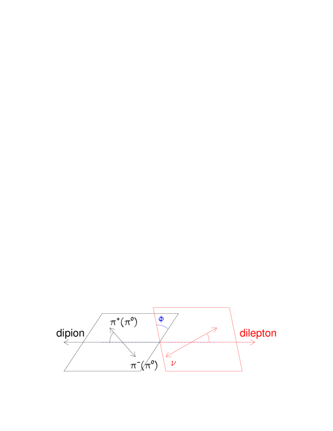
Figure 5: Sketch of the $\mathrm{K}_{\ell 4}$ decay in the kaon rest frame showing the definitions of $\theta$ and $\phi$ angles within and between the dipion and dilepton planes.

The decay amplitude is written as the product of the weak current of the leptonic part and the (V – A) current of the hadronic part:

$$\frac{G_{F}}{\sqrt{2}}V^{*}_{us}~{}\bar{u}_{\nu}\gamma_{\lambda}(1-\gamma_{5})v_{\ell}~{}\langle\mbox{$\pi^{+,0}$}\mbox{$\pi^{-,0}$}|V^{\lambda}-A^{\lambda}|\mbox{$K^{+}$}\rangle,\rm{~{}where}$$

$$\langle\mbox{$\pi^{+,0}$}\mbox{$\pi^{-,0}$}|A^{\lambda}|\mbox{$K^{+}$}\rangle= \displaystyle\frac{-i}{m_{K}}\left(F(\mbox{\boldmath$\mathrm{p}$}_{\mbox{$\pi^{+,0}$}}+\mbox{\boldmath$\mathrm{p}$}_{\mbox{$\pi^{-,0}$}})^{\lambda}+~{}G(\mbox{\boldmath$\mathrm{p}$}_{\mbox{$\pi^{+,0}$}}-\mbox{\boldmath$\mathrm{p}$}_{\mbox{$\pi^{-,0}$}})^{\lambda}+R(\mbox{\boldmath$\mathrm{p}$}_{\displaystyle\ell}+\mbox{\boldmath$\mathrm{p}$}_{\displaystyle\nu})^{\lambda}\right)\rm{~{}~{}~{}and}$$

$$\langle\mbox{$\pi^{+,0}$}\mbox{$\pi^{-,0}$}|V^{\lambda}|\mbox{$K^{+}$}\rangle= \displaystyle\frac{-H}{m_{K}^{3}}\epsilon^{\lambda\mu\rho\sigma}(\mbox{\boldmath$\mathrm{p}$}_{\mbox{$\pi^{+,0}$}}+\mbox{\boldmath$\mathrm{p}$}_{\mbox{$\pi^{-,0}$}}+\mbox{\boldmath$\mathrm{p}$}_{\displaystyle\ell}+\mbox{\boldmath$\mathrm{p}$}_{\displaystyle\nu})_{\mu}\hskip 145.10905pt$$ (2)

$$\hskip 85.35826pt\times~{}(\mbox{\boldmath$\mathrm{p}$}_{\mbox{$\pi^{+,0}$}}+\mbox{\boldmath$\mathrm{p}$}_{\mbox{$\pi^{-,0}$}})_{\rho}(\mbox{\boldmath$\mathrm{p}$}_{\mbox{$\pi^{+,0}$}}-\mbox{\boldmath$\mathrm{p}$}_{\mbox{$\pi^{-,0}$}})_{\sigma}.$$

In the above expressions, $\mathrm{p}$ refers to the four-momentum of the final state particles, $F,G,R$ are three axial-vector and $H$ one vector complex form factors with the convention $\epsilon^{0123}=1$. Note that $F,R$ are multiplied by terms symmetric with respect to the exchange of the two pions, while $G,H$ are multiplied by terms antisymmetric with respect to this same exchange.

The decay probability summed over lepton spins can be expressed as:

$$d^{5}\Gamma=\displaystyle\frac{G_{F}^{2}|V_{us}|^{2}}{2(4\pi)^{6}m_{K}^{5}}~{}\rho(\mbox{$S_{\pi}$},\mbox{$S_{\ell}$})~{}J_{5}(\mbox{$S_{\pi}$},\mbox{$S_{\ell}$},\mbox{$\theta_{\pi}$},\mbox{$\theta_{\ell}$},\phi)~{}d\mbox{$S_{\pi}$}~{}d\mbox{$S_{\ell}$}~{}d\mbox{$\cos\theta_{\pi}$}~{}d\mbox{$\cos\theta_{\ell}$}~{}d\phi,$$ (3)

where $\rho(\mbox{$S_{\pi}$},\mbox{$S_{\ell}$})=X\sigma_{\pi}\left(1-z_{\ell}\right)$ is the phase space factor, with $~{}X=\mbox{$\frac{1}{2}$}\lambda^{1/2}(m_{K}^{2},\mbox{$S_{\pi}$},\mbox{$S_{\ell}$}),\\ ~{}\sigma_{\pi}=(1-4m_{\pi}^{2}/\mbox{$S_{\pi}$})^{1/2},~{}\mbox{$z_{\ell}$}=m_{\ell}^{2}/\mbox{$S_{\ell}$},$ and $\lambda(a,b,c)=a^{2}+b^{2}+c^{2}-2(ab+ac+bc).$

The function $J_{5}$, displaying the angular dependencies on $\theta_{\ell}$ and $\phi$, reads [16, 3]:

$$J_{5}= 2(1-\mbox{$z_{\ell}$})(I_{1}+I_{2}~{}\mbox{$\cos 2\theta_{\ell}$}+I_{3}~{}\mbox{$\sin^{2}\theta_{\ell}$}\cdot\cos 2\phi+I_{4}~{}\mbox{$\sin 2\theta_{\ell}$}\cdot\mbox{$\cos\phi$}+I_{5}~{}\mbox{$\sin\theta_{\ell}$}\cdot\mbox{$\cos\phi$}$$ (4)

$$+I_{6}~{}\mbox{$\cos\theta_{\ell}$}+I_{7}~{}\mbox{$\sin\theta_{\ell}$}\cdot\mbox{$\sin\phi$}+I_{8}~{}\mbox{$\sin 2\theta_{\ell}$}\cdot\mbox{$\sin\phi$}+I_{9}~{}\mbox{$\sin^{2}\theta_{\ell}$}\cdot\sin 2\phi),$$

where

$\begin{array}[]{rl}I_{1}&=\mbox{$\frac{1}{4}$}\left((1+\mbox{$z_{\ell}$})|F_{1}|^{2}+\mbox{$\frac{1}{2}$}(3+\mbox{$z_{\ell}$})(|F_{2}|^{2}+|F_{3}|^{2})~{}\mbox{$\sin^{2}\theta_{\pi}$}+2\mbox{$z_{\ell}$}|F_{4}|^{2}\right),\vspace{2mm}\\ I_{2}&=-\mbox{$\frac{1}{4}$}(1-\mbox{$z_{\ell}$})\left(|F_{1}|^{2}-\mbox{$\frac{1}{2}$}(|F_{2}|^{2}+|F_{3}|^{2})~{}\mbox{$\sin^{2}\theta_{\pi}$}\right),\vspace{2mm}\\ I_{3}&=-\mbox{$\frac{1}{4}$}(1-\mbox{$z_{\ell}$})\left(|F_{2}|^{2}-|F_{3}|^{2}\right)~{}\mbox{$\sin^{2}\theta_{\pi}$},\vspace{2mm}\\ I_{4}&=\mbox{$\frac{1}{2}$}(1-\mbox{$z_{\ell}$})Re(F_{1}^{*}F_{2})~{}\mbox{$\sin\theta_{\pi}$},\vspace{2mm}\\ I_{5}&=-\left(Re(F_{1}^{*}F_{3})+\mbox{$z_{\ell}$}~{}Re(F_{4}^{*}F_{2})\right)~{}\mbox{$\sin\theta_{\pi}$},\vspace{2mm}\\ I_{6}&=-\left(Re(F_{2}^{*}F_{3})~{}\mbox{$\sin^{2}\theta_{\pi}$}-\mbox{$z_{\ell}$}~{}Re(F_{1}^{*}F_{4})\right),\vspace{2mm}\\ I_{7}&=-\left(Im(F_{1}^{*}F_{2})+\mbox{$z_{\ell}$}~{}Im(F_{4}^{*}F_{3})\right)~{}\mbox{$\sin\theta_{\pi}$},\vspace{2mm}\\ I_{8}&=\mbox{$\frac{1}{2}$}(1-\mbox{$z_{\ell}$})~{}Im(F_{1}^{*}F_{3})~{}\mbox{$\sin\theta_{\pi}$},\vspace{2mm}\\ I_{9}&=-\mbox{$\frac{1}{2}$}(1-\mbox{$z_{\ell}$})~{}Im(F_{2}^{*}F_{3})~{}\mbox{$\sin^{2}\theta_{\pi}$}.\end{array}$

The $I_{1}$ to $I_{9}$ expressions carry the dependence on ($\mbox{$S_{\pi}$},~{}\mbox{$S_{\ell}$},~{}\mbox{$\theta_{\pi}$}$) using the form factors ($F_{i},i=1,4$), combinations of the complex hadronic form factors $F,~{}G,~{}R,~{}H$ defined in Eq. (6).

In $\mathrm{K}_{\mathrm{e}4}$ decays, the electron mass can be neglected $(\mbox{$z_{\ell}$}=0)$ and the terms $(1\pm\mbox{$z_{\ell}$})$ become unity. One should also note that the form factor $F_{4}$ is always multiplied by $z_{\ell}$ and thus does not contribute to the full expression.

In the case of the neutral pion mode, there is no unambiguous definition of the $\theta_{\pi}$ angle as the two $\pi^{0}$ cannot be distinguished. The form factors $F_{2}=\sigma_{\pi}(\mbox{$S_{\pi}$}\mbox{$S_{e}$})^{1/2}G$ and $F_{3}=\sigma_{\pi}X\left(\mbox{$S_{\pi}$}\mbox{$S_{e}$}\right)^{1/2}H/m_{K}^{2}$ are related to the $G,H$ form factors of the decay amplitude, antisymmetric in the exchange of the two pions and therefore of null values.

With this simplification, there is a single complex hadronic form factor $F_{1}=XF+\mbox{$\frac{1}{2}$}\sigma_{\pi}(m_{K}^{2}-\mbox{$S_{\pi}$}-\mbox{$S_{e}$})~{}\mbox{$\cos\theta_{\pi}$}~{}G$ in the expression of $J_{5}$ which then reads $F_{1}=XF$, symmetric in the exchange of the two pions. At leading order, only the S-wave component of the partial wave expansion contributes ($F\equiv m_{K}^{2}F_{s}$ where $F_{s}$ is dimensionless).

The integration over the variables $\cos\theta_{\pi}$ and $\phi$ is trivial and Eqs. (3, 4) become:

$$d^{3}\Gamma =\displaystyle\frac{G_{F}^{2}|V_{us}|^{2}}{4(4\pi)^{5}m_{K}^{5}}~{}\rho(\mbox{$S_{\pi}$},\mbox{$S_{e}$})~{}J_{3}(\mbox{$S_{\pi}$},\mbox{$S_{e}$},\mbox{$\cos\theta_{e}$})~{}d\mbox{$S_{\pi}$}~{}d\mbox{$S_{e}$}~{}d\mbox{$\cos\theta_{e}$},$$

$$J_{3} =\mbox{$\frac{1}{2}$}|XF|^{2}(1-\mbox{$\cos 2\theta_{e}$})=m_{K}^{4}|XF_{s}|^{2}\mbox{$\sin^{2}\theta_{e}$}.\phantom{~{}d\mbox{$S_{\pi}$}~{}d\mbox{$S_{e}$}~{}d\mbox{$\cos\theta_{e}$}}$$ (5)

The differential rate depends on a single form factor $F_{s}$ whose variation with ($S_{\pi}$, $S_{e}$) is unknown and will be studied.

7 Acceptance calculation

A detailed GEANT3-based [17] Monte Carlo (MC) simulation is used to compute the acceptance for signal and normalization channels. It includes full detector geometry and material description, stray magnetic fields, DCH local inefficiencies and misalignment, LKr local inefficiencies, accurate simulation of the kaon beam line (reproducing the observed flux ratio $\mbox{$K^{+}$}/\mbox{$K^{-}$}\sim 1.8$) and time variations of the above throughout the running period. This simulation is used to perform two time-weighted MC productions, $10^{8}$ generated decays each, large enough to obtain the acceptances with a relative precision of few $10^{-4}$.

The signal channel $\mathrm{K}_{\mathrm{e}4}^{00}$ is generated according to Eq. (6) including a constant $F_{s}$ form factor. It can be reweighted according to another description of the form factor as obtained for example in Ref. [11] or in this analysis. The chosen form factor value is then propagated to the acceptance calculation by means of the same reweighting procedure. Going from a constant form factor value to the energy dependent value measured in Ref. [11], the relative signal acceptance change is $-1\%$.

The normalization channel $\mathrm{K}_{3\pi}^{00}$ is well understood in terms of simulation, being of primary physics interest to NA48/2 [18]. The most precise description of the decay amplitude has been implemented. This description corresponds to an empirical parameterization of the data [19] which includes the cusp-like shape of the $\pi^{0}$$\pi^{0}$ invariant mass squared at the $4m_{\pi^{+}}^{2}$ threshold and $\pi\pi$ bound states (Fig. 6).

Figure 6: (a) Cusp-like modification to the $\pi^{0}$$\pi^{0}$ invariant mass squared as introduced in the simulation, normalized to the classical series expansion in $M_{\pi^{0}\pi^{0}}^{2}$. (b) Distributions of the $\pi^{0}$$\pi^{0}$ invariant mass squared for reconstructed data and simulated events. The arrow points to the $4m_{\pi^{+}}^{2}$ value.

Depending on the data taking conditions, the relative acceptance variation can be as large as 5% for both signal and normalization channels due to the faulty HOD slabs but the ratio $A_{n}/A_{s}$ stays within $\pm 0.4\%$ of its average value.

The same selection and reconstruction as described in Section 4 are applied to the simulated events except for the trigger and timing requirements. Particle identification cuts related to the LKr response are replaced by momentum-dependent efficiencies, obtained from data in pure samples of electron tracks (Fig. 1a).

Real photon emission using PHOTOS 2.15 [20] is included in both $\mathrm{K}_{\mathrm{e}4}^{00}$ and $\mathrm{K}_{3\pi}^{00}$ simulations. It distorts the original $M_{e\nu}$ distribution and consequently modifies the overall acceptance. A dedicated study with and without photon emission was performed on a subset of the simulation sample. The $\mathrm{K}_{3\pi}^{00}$ acceptance is unaffected while a relative acceptance change of $-2\%$ is observed for $\mathrm{K}_{\mathrm{e}4}^{00}$ when real photon emission is implemented. Details of the photon emission modeling will be discussed together with other systematic uncertainties.

The acceptance values, averaged on both kaon charges and over the data-taking periods, are $A_{s}=(1.926\pm 0.001)\%$ and $A_{n}=(4.052\pm 0.002)\%$. The $A_{s}$ variations from 0 to about 4% ($A_{n}$ from 0 to about 9%) across the Dalitz plot are shown in Fig. 7.

Figure 7: Acceptance of (a) $\mathrm{K}_{\mathrm{e}4}^{00}$ candidates in the plane ($\mbox{$M_{\pi\pi}$},\mbox{$M_{e\nu}$}$) and of (b) $\mathrm{K}_{3\pi}^{00}$ candidates in the plane ($u,|v|$). The dimensionless variables ($u,|v|$) are defined as $u=(M_{\pi^{0}\pi^{0}}^{2}-s_{0})/m_{\pi^{+}}^{2}$ and $|v|=|M_{\pi^{+}\pi^{0}_{1}}^{2}-M_{\pi^{+}\pi^{0}_{2}}^{2}|/m_{\pi^{+}}^{2}$ with $s_{0}=(m_{K^{+}}^{2}+2m_{\pi^{0}}^{2}+m_{\pi^{+}}^{2})/3$. The notation $\pi^{0}_{1},\pi^{0}_{2}$ is only used to distinguish one $\pi^{0}$ from the other but has no particular meaning beyond this.

8 Trigger efficiency

Both signal and normalization modes are recorded concurrently with the same trigger logic. Downscaled minimum bias control triggers are used to measure the efficiency of the main trigger channels. Hardware changes to the trigger conditions were introduced during data taking following improvements in detector and readout electronics performance. As a consequence, trigger effects have been studied separately for data samples taken during ten periods of stable trigger conditions. Details of the trigger efficiency for normalization events are given in Refs. [13, 21]. As described in Section 2, $\mathrm{K}_{3\pi}^{00}$ and $\mathrm{K}_{\mathrm{e}4}^{00}$ events were recorded by a first level trigger using signals from HOD (Q1) and LKr (NUT), followed by a second level trigger using DCH information (MBX). Using event samples recorded with downscaled control triggers, and selecting $\mathrm{K}_{3\pi}^{00}$ and $\mathrm{K}_{\mathrm{e}4}^{00}$ decays as described in Section 4, it is possible to measure separately two efficiencies:

- the efficiency of the NUT trigger using a sample recorded by the Q1$\cdot$MBX trigger;

- the efficiency of the Q1$\cdot$MBX trigger using a sample recorded by the NUT trigger.

These two efficiencies rely on different detector information and are statistically independent. They are multiplied to obtain the overall trigger efficiency of each subsample for both signal and normalization channels.

NUT trigger efficiency. In the $\mathrm{K}_{3\pi}^{00}$ selection, the inefficiency is measured to be 0.5% (most of 2003), 3% (end of 2003 and beginning of 2004) and then $3\times 10^{-4}$ until the end of 2004. Because of the extra LKr energy deposit from the electron, this inefficiency is even smaller in the $\mathrm{K}_{\mathrm{e}4}^{00}$ selection than in the $\mathrm{K}_{3\pi}^{00}$ selection. In each data taking period, the control trigger sample is large enough to determine the efficiency with an excellent precision ${\cal O}(10^{-4})$ for the normalization sample and a precision better than $5\times 10^{-3}$ in the signal sample.

Q1$\cdot$MBX trigger efficiency. The inefficiency suffers from somewhat large variations with data taking conditions, ranging from 3% to 7% due to local DCH inefficiencies. Control samples are large enough in the $\mathrm{K}_{3\pi}^{00}$ selection to determine the efficiency within a few $10^{-4}$ precision. In the signal selection, there are too few control triggers in 2003 to ensure a precise enough efficiency measurement. As the uniformity of the Q1 trigger part is ensured by HOD geometrical fiducial cuts in the selection, the lack of statistics is overcome by taking advantage of the realistic simulation code of the MBX algorithm that proves to reproduce accurately the efficiency variations in the $\mathrm{K}_{3\pi}^{00}$ selection, as measured from the data. The MBX efficiency for the signal mode is therefore obtained from the MBX simulation. The Q1$\cdot$MBX efficiency values are in very good agreement with the measured values but obtained with improved precision.

The statistical average of the Q1$\cdot$NUT$\cdot$MBX trigger efficiency over the ten independent samples is $(96.06\pm 0.03)\%$ for the $\mathrm{K}_{\mathrm{e}4}^{00}$ selection and $97.42\%$ with a negligible error for the $\mathrm{K}_{3\pi}^{00}$ selection.

9 Form factor measurement

9.1 Measurement method

The form factor study requires a sample free of large radiative effects which can pollute the original kaon decay amplitude. An extra cut is applied in the signal selection (Section 4), rejecting events where an additional photonic energy deposit is identified with at least $3~{}\mbox{$\mathrm{GeV}$}$ energy, in-time with the signal candidate track and photons, and away by more than 15 cm from the track impact at LKr and 10 cm from each of the four photons forming the two $\pi^{0}$ candidates. This reduces the number of selected signal candidates from 65210 to 65073 and the estimated number of background events from 650 to 641.

The event density in the $(\mbox{$S_{\pi}$},\mbox{$S_{e}$})$ plane, also called the Dalitz plot, is proportional to $F_{s}^{2}$ as shown in Eq. (6). The number of events in the $(\mbox{$S_{\pi}$},\mbox{$S_{e}$})$ plane and the projected distributions along the two variables are displayed in Fig. 8. The Dalitz plot density is compared, after background subtraction, to the density obtained from the simulation where kinematics, acceptance, resolution, trigger efficiency, and radiative effects are taken into account.

To analyze the data as a single sample while reproducing the variation of data taking conditions in the simulation as closely as possible, the simulated sample should reflect:
- the time dependence of the number of kaon decays in each data sample;
- the relative variation of the trigger efficiency across the Dalitz plot;
- the measured Q1$\cdot$NUT$\cdot$MBX trigger efficiency in each subsample.

To that purpose, the integrated number of kaon decays in each subsample is obtained from the number of observed normalization candidates corrected for the selection acceptance, the trigger efficiency and the known branching ratios [10]. The numbers of $\mathrm{K}_{\mathrm{e}4}^{00}$ signal events generated for each subsample is the same up to an arbitrary scale factor reflecting the fraction of the total number of kaon decays generated. A fine tuning of the generated subsample sizes results in applying similar weights to all subsamples, in the range 0.9 to 1.

No particular pattern is observed in the Dalitz plot for the inefficient NUT triggers. The Q1 trigger efficiency is known to be very high $(>99.75\%$ as measured in other studies [13]) and uniform once the local inefficient areas have been excluded by the event selection. The dependence of the MBX trigger efficiency on $S_{\pi}$ can be studied from $\mathrm{K}_{3\pi}^{00}$ data control triggers and simulated samples. Because of different local DCH inefficiencies, different subsamples may have non-identical variations. However the variations observed in the data are well reproduced in the simulation within a $\pm 1\%$ relative accuracy. This justifies the usage of the simulation code as being realistic also for the $\mathrm{K}_{\mathrm{e}4}^{00}$ signal.

Once local variations have been considered, a fine tuning of the overall trigger efficiency of each simulated subsample is achieved by applying weights with values between 0.98 and 1.

9.2 Fitting procedure and results

Given the size of the data sample, a grid is defined with ten equal population bins ($\sim 5900$ candidates per box) in the interval $\mbox{$S_{\pi}$}>4m_{\pi^{+}}^{2}$ and two equal population bins ($\sim 2900$ candidates per box) in the interval $\mbox{$S_{\pi}$}<4m_{\pi^{+}}^{2}$. Along the $S_{e}$ variable, ten bins of unequal width, common to all $S_{\pi}$ bins, are defined. Eight boxes outside the kinematic boundary are not populated and excluded from the fit (Fig. 8a).

Figure 8: (a) Distribution of $\mathrm{K}_{\mathrm{e}4}^{00}$ candidates in the plane ($\mbox{$S_{\pi}$},\mbox{$S_{e}$}$). The dotted lines represent the binning used in the fit procedure. Distribution of $\mathrm{K}_{\mathrm{e}4}^{00}$ candidates in the $S_{\pi}$ (b) and $S_{e}$ (c) variables after background subtraction (dots). Background, multiplied by a factor of ten to be visible, is displayed as a histogram.

Dimensionless variables may also be used to describe the Dalitz plot, dividing $S_{\pi}$ and $S_{e}$ by $4m_{\pi}^{2}$ with the arbitrary choice of using either $m_{\pi^{+}}$ or $m_{\pi^{0}}$. A natural choice would be to use $m_{\pi^{0}}$. For a direct comparison with the $\mathrm{K}_{\mathrm{e}4}^{+-}$ mode, it is however more appropriate to choose $m_{\pi^{+}}$. The following variables are defined: $q^{2}=(\mbox{$S_{\pi}$}/4m_{\pi^{+}}^{2}-1){\rm~{}and~{}}y^{2}=\mbox{$S_{e}$}/4m_{\pi^{+}}^{2}.$ The allowed kinematic range of $q^{2}$ for the $\mathrm{K}_{\mathrm{e}4}^{00}$ decay spans both positive and negative values. In a first approach, without any prior knowledge of the energy dependence, an empirical parameterization (often called “model independent”) is used to describe the ratio of the data and simulated Dalitz plots. The ratio of the two distributions is equal to unity when the total number of simulated events, weighted for the best values of fit parameters, is normalized to the total number of data events after background subtraction. This ratio corresponds to $(F_{s}/f_{s})^{2}$ where $f_{s}$ is a constant which can be determined using the branching ratio measurement (see Section 11). The fit procedure minimizes a $\chi^{2}$ expression in the two-dimensional space:

$$\chi^{2}=\sum_{i=1}^{12}\sum_{j=1}^{10}((n_{ij}/m_{ij}-{\cal F}(q^{2}_{i},y^{2}_{j},\hat{p}))/\sigma_{ij})^{2},$$

where $n_{ij}$ is the number of background subtracted data events in the box $ij$, $m_{ij}$ is the number of simulated events observed in the same box for a constant form factor, $\hat{p}$ is the set of fit parameters and $\sigma_{ij}$ is the statistical uncertainty on the ratio, taking both data and simulation statistics into account. The sum runs over the 112 boxes in the $(q^{2},y^{2})$ space (12 bins along $q^{2}$ and 10 along $y^{2}$, excluding the 8 non-populated boxes). The fit function ${\cal F}(q^{2},y^{2},{\hat{p}})$ is defined as:

$${\cal F}(q^{2},y^{2},{\hat{p}})=\begin{cases}N(1+a~{}q^{2}+b~{}q^{4}+c~{}y^{2})^{2}&{\rm~{}for~{}}q^{2}\geq 0\\ N(1+d~{}C(q^{2})+c~{}y^{2})^{2}&{\rm~{}for~{}}q^{2}<0\end{cases}~{},$$ (6)

where the fit parameters ${\hat{p}}$ are $(a,b,c,d$). The cusp-like function $C(q^{2})$ is defined as $C(q^{2})=\sqrt{|q^{2}/(1+q^{2})|}$ and $N$ is a normalization parameter. At each step of the fit, the function ${\cal F}$ is evaluated in each box at the corresponding reconstructed barycenter position $(q^{2}_{i},y^{2}_{i})$ using the ’true’ $(q^{2},y^{2})$ values. The results from the 2-dimensional fit are given in Table 1. The correlation matrix is symmetric and its non-diagonal terms are quoted in Table 2.

If the $S_{e}$ dependence is neglected ($c=0$), the fit quality becomes worse ($\chi^{2}/ndf=129.8/108$, with a 7% probability). The results of such a fit are different from those obtained when considering a dependence on $S_{e}$ and the degraded $\chi^{2}$ value supports the inclusion of an additional fit parameter. Other fits considering only data above $q^{2}=0$ have also been performed with consistent results. Omitting the $S_{e}$ dependence below $q^{2}=0$ brings a small increase of the $\chi^{2}$ value ($\chi^{2}/ndf$ becomes 107.9/107 with a reduced $46\%$ probability compared to Table 1). Allowing the $S_{e}$ dependence to be different above and below $q^{2}=0$ leads to very close values with larger errors and no $\chi^{2}$ improvement. Therefore the formulation of Eq. (6) with an identical $y^{2}$ dependence below and above $q^{2}=0$ is considered in the final result.

Table 1: Result of the fit to the Dalitz plot. The coefficients are defined in Eq. (6). The errors are statistical only.

fit parameters	values
$a$	$0.149\pm 0.033$
$b$	$-0.070\pm 0.039$
$c$	$0.113\pm 0.022$
$d$	$-0.256\pm 0.049$
$N$	$0.0342\pm 0.0004$
$\chi^{2}/ndf$	$101.4/107=0.95$
probability	$63\%$

Table 2: Non-diagonal correlation coefficients between the two-dimensional fit parameters.

	$a$	$b$	$c$	$d$
$N$	$-0.751$	$0.581$	$-0.644$	$-0.417$
$a$		$-0.946$	$0.180$	$0.467$
$b$			$-0.062$	$-0.400$
$c$				$-0.028$

For a simpler display, the projection of the Dalitz plot on the $q^{2}$ variable is shown in Fig. 9 for data and simulation (generated with a constant form factor). As the $q^{2}$ distribution is very steep at negative values, the comparison is also shown as the ratio of the two distributions in equal population bins: the statistical errors are identical for the last 10 equal population bins and larger by a factor of $\sqrt{2}$ for the first two bins (half population).

Figure 9: (a) Data and simulation (including a constant form factor) $q^{2}$ distributions $(q^{2}=\mbox{$S_{\pi}$}/4m_{\pi^{+}}^{2}-1)$. (b) Ratio of the two $q^{2}$ distributions in equal population bins. Each symbol is plotted at the barycenter position of the data events in the bin to account correctly for the variable size binning. The line corresponds to the empirical description using the best fit-parameter values: a degree-2 polynomial above $q^{2}=0$ and a cusp-like function below.

The results in the $(q^{2},y^{2})$ formulation can be directly compared to those obtained in the $\mathrm{K}_{\mathrm{e}4}^{+-}$ analysis [11] where the corresponding form factor is described as $F_{s}=f_{s}(1+f^{\prime}_{s}/f_{s}~{}q^{2}+f^{\prime\prime}_{s}/f_{s}~{}q^{4}+f^{\prime}_{e}/f_{s}~{}y^{2})$. They are displayed in Fig. 10 in the three 2-parameter planes.

Figure 10: Form factor description in 2-parameter planes obtained in $\mathrm{K}_{\mathrm{e}4}^{00}$ and $\mathrm{K}_{\mathrm{e}4}^{+-}$ analyses in the $(q^{2},y^{2})$ series expansion formulation. The top plot corresponds to the $(f^{\prime}_{s}/f_{s},f^{\prime\prime}_{s}/f_{s})$ plane (the $(a,b)$ plane), the bottom plots to the $(f^{\prime}_{s}/f_{s},f^{\prime}_{e}/f_{s})$ and $(f^{\prime\prime}_{s}/f_{s},f^{\prime}_{e}/f_{s})$ planes (the $(a,c)$ and $(b,c)$ planes, respectively). Errors plotted are statistical only and all contours are $68\%$ CL. The smaller area corresponds to the $\mathrm{K}_{\mathrm{e}4}^{+-}$ result obtained from a large statistical sample [11]. The correlations between fitted parameter errors are very similar and results are consistent within statistical errors.

9.3 Systematic uncertainties

Many possible sources of systematics uncertainties have been explored and details are given for the main contributions.

Background control. Background has been studied both in shape and rate across the Dalitz plot. The most sensitive item is the fake-electron background from $\mathrm{K}_{3\pi}^{00}$.

The shape of the background can be modified by extending further out the ellipse cut in the $(M_{3\pi},p_{t})$ plane (Section 4): due to the location of the fake-electron background close to the ellipse cut boundary, its fraction varies rapidly from 0.65% to 0.50%, 0.39% and 0.31% when increasing the ellipse main axes by 10%, 20% and 30% of their nominal values while the signal loss (estimated from simulation) is 1.2%, 2.7% and and 4.4%, respectively. This changes both the rate and the shape of the fake-electron background while the relative fraction of background from $\mbox{$\pi^{\pm}$}\rightarrow e^{\pm}\nu$ decays (0.12%) and accidentals (0.22%) are unaffected.

The use of looser or tighter electron-identification criteria is another way to vary the background contribution both in shape and relative rate. The efficiency of the DV cut as a function of the cut value is well known from previous studies [11, 12]. When changing the cut value from 0.90 (reference) to 0.85 (0.95), the number of candidates changes by $+1.1\%~{}(-2.8\%)$, the fraction of fake-electrons relative to signal changes from 0.65% to 0.78% (0.47%) while the relative fraction of decay-electrons remains unchanged (0.12%). Conservatively, the maximum difference observed between any of the five fit results and the reference value is quoted as a systematic uncertainty, not taking into account the large anti-correlation between parameters $a$ and $b$ (Table 2). The quoted contribution is then ${\cal O}(1\times 10^{-2})$ for all parameters.

The extrapolation method (Section 5) using a single scaling factor or a momentum dependent factor has little impact (few $10^{-4}$) as the momentum spectra of control regions C and D are very similar.

The fit parameters vary linearly with the rate of each background component as observed when scaling each nominal component by a factor of 0, 0.5, 1, 2 while keeping its shape unchanged. The fake-electron background ($425\pm 2$ events) is known to better than 1%, the decay-electron component ($79\pm 1$ events) is known to about 1% and the accidental background ($146\pm 13$ events) to about 10%. The uncertainty related to each background scale is a few $10^{-4}$ (or less) for all parameters.

All considered contributions are then added in quadrature and the sum quoted in Table 3.

Radiative events modeling. The $\mathrm{K}_{\mathrm{e}4}^{00}$ final state contains at least four photons. To evaluate how the presence of additional photons can distort the measurement (either from Inner Bremsstrahlung (IB) at the decay vertex or from External Bremsstrahlung (EB) emitted in the interaction of the $e^{\pm}$ with matter), dedicated simulated samples without IB (or EB) photon emission have been analyzed as real data.

Other studies [22] have shown that the material description before the spectrometer magnet in terms of radiation length is known within 1.1% precision. One percent of the full effect observed when omitting EB is quoted as a systematic error of few $10^{-4}$ for all parameters.

As reported by the PHOTOS authors in Ref. [23], the IB modeling uncertainty should not exceed 10% of the full effect. Therefore 10% of the difference between the results obtained with and without IB is quoted as an uncertainty on the photon emission modeling with a few ${\cal O}(1\times 10^{-3})$ contribution for all fit parameters. Both EB and IB contributions are added in quadrature, dominated by the IB modeling uncertainty.

Others. The analysis of simulated samples, different from those used in the fit and treated as real data, has not revealed any bias in the fit procedure. The variation of the chosen grid in $S_{e}$ has no significant impact on the fit results.

Applying more stringent criteria in the reconstruction, excluding either 5% of candidates having more than one vertex solution, or 1.2% of candidates with no available track HOD time, or up to 20% of candidates with a reconstructed $M_{e\nu}$ value lower than 60 $\mathrm{MeV}/{{\it c}^{2}}$ (affected by a worse resolution), shows no significant effect on the fit results.

When the corrections applied to the simulation samples are removed in turn, the only sizable change is observed when omitting the variation of the MBX trigger across the Dalitz plot. The studies of abundant $\mathrm{K}_{3\pi}^{00}$ events have shown a good agreement between data and simulation within 1%. One percent of the difference between the results obtained with and without MBX trigger simulation is quoted as systematic uncertainty.

The offline $M_{miss}$ cut is chosen to be more strict than the online trigger requirement to guarantee high efficiency. Moving further away from the nominal cut (206 $\mathrm{MeV}/{{\it c}^{2}}$, see Section 4) to 217, 227 and 237 $\mathrm{MeV}/{{\it c}^{2}}$, the signal statistics decreases by 5.4%, 11% and 17%, respectively. The fit results are in agreement with the nominal analysis results within the statistical errors and with no definite trend.

Acceptance control stability. Stability checks are performed by splitting the data sample into statistically independent subsamples and comparing fit results. Two independent subsamples are defined according to each quantity to keep statistical errors low enough and the split is repeated for many different quantities. These studies investigate possible biases from lack of control of the beam geometry (achromat polarity, kaon beam charge), the spectrometer and calorimeter response (spectrometer magnet polarity, regions of LKr geometrical illumination from track transverse position), the detector geometry (vertex $Z$ position) and their overall time variation (year). The 14 fits are obtained with a good quality $\chi^{2}$ and the parameter variations are consistent within the increased statistical error and the correlation matrix.

A summary of all contributions from studied effects is given in Table 3. The main contribution comes from the background control while the radiative events modeling contribution is much smaller. Other sources give marginal contributions.

Table 3: Systematic uncertainty contributions to the form factor description. The parameter values and their statistical error are also recalled for completeness.

Source	$\delta a$	$\delta b$	$\delta c$	$\delta d$
Background control	0.0140	0.0122	0.0062	0.0164
Radiative events modeling	0.0037	0.0035	0.0033	0.0013
Fit procedure	–	–	–	–
Reconstruction/resolution	–	–	–	–
Trigger simulation	$<0.0001$	$<0.0001$	$<0.0001$	$<0.0001$
Acceptance control	–	–	–	–
Total systematics	00.014	-0.013	00.007	-0.016
Parameter	$a$	$b$	$c$	$d$
Value	0.149	$-0.070$	0.113	$-0.256$
Statistical error	0.033	$\phantom{-}0.039$	0.022	$\phantom{-}0.049$

9.4 Discussion

The observed deficit of events at $q^{2}<0$ can be related to the final state charge exchange scattering process $(\mbox{$\pi^{+}$}\mbox{$\pi^{-}$}\rightarrow\mbox{$\pi^{0}$}\mbox{$\pi^{0}$})$ in the $\mathrm{K}_{\mathrm{e}4}^{+-}$ decay mode. In a naive and qualitative approach, one may take advantage of the early one-loop description of re-scattering effects in the $\mathrm{K}_{3\pi}^{00}$ mode [24] and consider a similar interpretation in the $\mathrm{K}_{\mathrm{e}4}^{00}$ decay mode, defining the tree level amplitude ${\cal M}_{0}$ and the one-loop amplitude ${\cal M}_{1}$ (Fig. 11) of the $\mathrm{K}_{\mathrm{e}4}^{00}$ mode.

Figure 11: (a) Tree level diagram (amplitude ${\cal M}_{0}$) for the $\mathrm{K}_{\mathrm{e}4}^{00}$ decay mode. (b) One-loop diagram (amplitude ${\cal M}_{1}$) with contribution of the $\mathrm{K}_{\mathrm{e}4}^{+-}$ decay mode to the $\mathrm{K}_{\mathrm{e}4}^{00}$ final state.

The tree level amplitude ${\cal M}_{0}$ has a dispersive behavior above and below $q^{2}=0$. The one-loop amplitude ${\cal M}_{1}$ is imaginary for $q^{2}>0$ $(i{\cal M}_{1})$ and real for $q^{2}<0$ $({\cal M}_{1})$. It has two components: a dispersive component which can be absorbed in the unperturbed amplitude ${\cal M}_{0}$ and a negative absorptive component. The total amplitude squared is then written as:

$$|{\cal M}|^{2}=\begin{cases}|{\cal M}_{0}+i{\cal M}_{1}|^{2}=({\cal M}_{0})^{2}+({\cal M}_{1})^{2}&q^{2}>0\\ |{\cal M}_{0}+~{}{\cal M}_{1}|^{2}=({\cal M}_{0})^{2}+({\cal M}_{1})^{2}+2{\cal M}_{0}{\cal M}_{1},&q^{2}<0\end{cases}~{}.$$

In this approximate approach, neglecting a potential $S_{e}$ dependence, ${\cal M}_{0}$ can be developed in a series expansion in $q^{2}$ (as described for $q^{2}>0$ in the form factor measurement in Section 9 and Table 1) and ${\cal M}_{1}$ can be expressed as:

$${\cal M}_{1}=-2/3~{}(a_{0}^{0}-a_{0}^{2})~{}F^{+-}_{s}~{}\sigma_{\pi}(q^{2}),$$

where $F^{+-}_{s}=f^{+-}_{s}(1+f^{\prime}_{s}/f_{s}~{}q^{2}+f^{\prime\prime}_{s}/f_{s}~{}q^{4})$ is the $\mathrm{K}_{\mathrm{e}4}^{+-}$ form factor [11], $a_{0}^{0}$ and $a_{0}^{2}$ are the S-wave $\pi\pi$ scattering lengths in the isospin states $I=0$ and $I=2$, while $\sigma_{\pi}(q^{2})=\sqrt{1-4m_{\pi^{+}}^{2}/\mbox{$S_{\pi}$}}=\sqrt{|q^{2}/(1+q^{2})|}$ introduces, through the interference term below $q^{2}=0$, a cusp-like behavior as observed in the data.

Better descriptions of re-scattering effects in the $\mathrm{K}_{3\pi}^{00}$ decay amplitude already exist, including two-loop effects [25] and also radiative corrections within a ChPT calculation [26]. Recent developments on the related topic of the low energy pion form factors [27] may also bring a more elaborate description of the $\mathrm{K}_{\mathrm{e}4}^{00}$ amplitude including two-loop contributions, $\pi\pi$ scattering and mass related isospin symmetry breaking effects. Once available, such an approach could be exploited further to extract more information related to physical quantities from the result reported here.

10 Branching ratio measurement

10.1 Inputs

All input ingredients to the BR($\mathrm{K}_{\mathrm{e}4}^{00}$) measurement (Eq. (1)) are summarized in Table 4 for each kaon charge, summed over the ten subsamples (or averaged when appropriate) while the final result is obtained as the statistical average of the ten independent subsamples summed over both kaon charges (Fig. 12). Because of the symmetrization of the beam and detector geometries, the global $K^{+}$ and $K^{-}$ acceptances are very similar: $K^{+}$ and $K^{-}$ beam lines are exchanged when inverting the achromat polarity while positive and negative charged track trajectories follow similar paths in the spectrometer when inverting the spectrometer magnet polarity. Data taking conditions have been set up carefully to equalize the integrated kaon flux in the four configurations of achromat and spectrometer magnet polarities [13]. The acceptances $A_{s}$ and $A_{n}$ are obtained using the most elaborate description of the decay dynamics, in particular the model independent parameterization of the signal form factor reported here. The trigger efficiencies $\varepsilon_{n}$ ($\varepsilon_{s}$) are the product of the two measured trigger components NUT and Q1$\cdot$MBX. All quoted uncertainties are of statistical origin.

Table 4: Inputs to the BR($\mathrm{K}_{\mathrm{e}4}^{00}$) measurement for each kaon charge summed over subsamples. Uncertainties on the last digits are given in parentheses. The last two columns display the overall numbers and the contribution of each component to the relative branching ratio error.

	$K^{+}$	$K^{-}$	$K^{\pm}$	$\delta$BR/BR $(\times 10^{4})$
$N_{s}$	41 850	23 360	65 210	39
$N_{b}(s)$	418	233	651	4
$N_{n}$	60 107 311	33 436 659	93 543 970	1
$N_{b}(n)$	148 486	82 600	231 086	$\ll 1$
$A_{s}$	$1.927(2)\%$	$1.923(2)\%$	$1.926(1)\%$	5
$A_{n}$	$4.053(2)\%$	$4.047(3)\%$	$4.052(2)\%$	5
$\varepsilon_{s}$	$96.06(3)\%$			3
$\varepsilon_{n}$	$97.42(0)\%$			$\ll 1$
Total relative error				40

10.2 Systematic uncertainties

Some sources of uncertainty are expected to affect the corresponding quantities for signal and normalization modes in a similar way and therefore have a limited impact as they cancel at first order in the ratio of Eq. (1). Some others are specific to the signal or normalization mode.

Background in the $\mathrm{K}_{\mathrm{e}4}^{00}$ sample. The fake-electron component ($425\pm 2$ events) is obtained with an uncertainty from the extrapolation procedure of 0.4%. Conservatively, the half difference between the evaluations based on two control subregions (restricted to $E/p$ ranges from 0.2 to 0.45 and from 0.45 to 0.7, respectively, see Fig. 3) is assigned as an additional systematic error of $\pm 5$ events and added in quadrature. This background contributes $\delta$BR/BR $=1\times 10^{-4}$.

The uncertainty on the $\mbox{$\pi^{\pm}$}\rightarrow e^{\pm}\nu$ component ($79\pm 0.7$ events) is due to the limited statistics of the simulation and BR$(\mbox{$\mbox{$\pi^{\pm}$}\rightarrow e^{\pm}\nu$})$ precision, adding up to $0.8\%\oplus 0.3\%=0.9\%$. This contribution $\delta$BR/BR $=0.1\times 10^{-4}$ is marginal.

The accidental component precision ($146\pm 12$ events) is limited by the statistics of the side band signal sample. The statistical error is quoted as systematics and contributes $\delta$BR/BR $=2\times 10^{-4}$. Adding in quadrature the three contributions, the background systematic uncertainty is $\delta$BR/BR = $2.2\times 10^{-4}$.

An estimation of the uncertainty in the electron identification procedure is obtained from the stability of the result when varying the DV cut value between 0.85 and 0.95, changing the fake-electron background by a factor close to 2 (Fig. 1b). The analysis of the signal mode was repeated for three cut values (0.85, 0.90, 0.95) and the observed change quoted as $\delta$BR/BR = $25\times 10^{-4}$, the dominant contribution.

Radiative effects. The event selection requires a minimum track to photon and photon to photon distance at the LKr front face. The precise description of IB (EB) emission may affect the acceptance calculation.

Dedicated MC samples simulated without IB photon emission are used to estimate the impact of the PHOTOS description. The signal acceptance $A_{s}$ increases by $1.9\%$ while $A_{n}$ is unchanged. One tenth of the observed effect is assigned as a modeling uncertainty according to the prescription of Ref. [23], $\delta$BR/BR = $19\times 10^{-4}$.

Dedicated simulations including IB by PHOTOS, but switching off EB in the GEANT tracking in the detector, show that $A_{n}$ is unaffected (within the simulated statistics) while $A_{s}$ increases by $(3.5\pm 0.4)\%$. The agreement between data and simulation in term of radiation length is quoted as 1% as studied in Ref. [22]. This fraction of the observed change is propagated as $\delta$BR/BR = $4\times 10^{-4}$ and is added in quadrature to the dominant IB-related uncertainty.

Form factor description in the $\mathrm{K}_{\mathrm{e}4}^{00}$ simulation. The signal acceptance $A_{s}$ calculation depends on the form factor description considered in the simulation. When using $F_{s}$ descriptions from NA48/2 $\mathrm{K}_{\mathrm{e}4}^{+-}$ [11] or $\mathrm{K}_{\mathrm{e}4}^{00}$ (present work) modes, $A_{s}$ changes by less than 0.01% consistent with no change within the corresponding statistical precision. Both descriptions are in agreement while the $\mathrm{K}_{\mathrm{e}4}^{+-}$ form factor coefficients are obtained with better precision (Fig. 10). Moving each coefficient in turn by $\pm 1\sigma$ away from its measured value, the corresponding acceptance variations are obtained. Conservatively (i.e. neglecting the anti-correlation between the $a,b$ fit parameters), these $A_{s}$ variations related to the $a,b,c$ coefficients in the $\mathrm{K}_{\mathrm{e}4}^{+-}$ mode [11] are added in quadrature. The major contributions come from $a$ and $b$ parameter variations. The acceptance has about three times less sensitivity to the $c$ coefficient and about twelve times less to the $d$ coefficient. Therefore including or not the $d$ contribution does not change the quoted uncertainty $\delta$BR/BR = $17\times 10^{-4}$.

Acceptance stability. Many stability checks have been performed varying the selection cuts. The acceptances $A_{s}$ and $A_{n}$ are particularly sensitive to the minimum radial track position at DCH1 ($R_{CH1}$). When increasing $R_{CH1}$ by steps of 1 cm, the number of $\mathrm{K}_{\mathrm{e}4}^{00}$ candidates decreases by steps of about 3% and the number of $\mathrm{K}_{3\pi}^{00}$ candidates by larger steps of about 4%. Changes in acceptance and number of candidates largely compensate each other in the BR calculation. Therefore only the largest significant difference is quoted as the corresponding uncertainty, $\delta$BR/BR = $16\times 10^{-4}$.

The control level of the time variation of the acceptance is estimated by swapping the acceptances (obtained from simulation) of pairs of subsamples recorded during different time periods. This leads to a conservative estimate $\delta$BR/BR = $4\times 10^{-4}$.

The stability of the BR value with the spectrometer magnet polarity (B⁺, B^-), the achromat polarity (A⁺, A^-), the year of data taking (2003, 2004) or the kaon charge (K⁺, K^-) has not revealed any significant effect.

The above effects are combined into $\delta$BR/BR = $16\times 10^{-4}$.

Level 2 trigger cut. Varying the $M_{miss}$ cut applied in the selection and recomputing both acceptances and trigger efficiencies provide an estimate of the uncertainty related to the trigger cut. Moving the cut value from 206 to 227 $\mathrm{MeV}/{{\it c}^{2}}$ in the selection, the acceptance, trigger efficiency and number of candidates in the normalization sample are unaffected. The signal statistics decreases by 12.5% at no gain in the trigger efficiency and therefore will only increase the statistical error by 6%. The difference between the branching ratio values obtained for both cut values is quoted as a systematic uncertainty $\delta$BR/BR = $4\times 10^{-4}$.

Beam geometry modeling and resolution. The comparison of the reconstructed parent kaon momentum distributions of data and simulated $\mathrm{K}_{3\pi}^{00}$ candidates can be used to improve the beam geometry modeling. This fine tuning of the beam properties is propagated to the $\mathrm{K}_{\mathrm{e}4}^{00}$ simulation. As the selection cuts are loose enough, there is little sensitivity to these mismatches and the observed change of $A_{s}$ is negligible.

Spectrometer and calorimeter calibrations. The study of the mean reconstructed $\mathrm{K}_{3\pi}^{00}$ mass as a function of the charged pion momentum and of the photon energies is an indication of the level of control of the spectrometer momentum calibration and the calorimeter energy calibration.

Both data and simulated reconstructed $M_{3\pi}$ distributions show a similar residual variation with the charged pion momentum, which indicates that the momentum calibration could still be improved. However, the maximum effect of $\pm 0.35~{}\mbox{$\mathrm{MeV}/{{\it c}^{2}}$}$ is well below the achieved resolution of $1.4~{}\mbox{$\mathrm{MeV}/{{\it c}^{2}}$}$. The residual variations with the photon energies are also similar for data and simulated samples and within $\pm 0.35~{}\mbox{$\mathrm{MeV}/{{\it c}^{2}}$}$, consistent with a relative change in energy scale smaller than $1\times 10^{-3}$. No additional systematic uncertainty is assigned.

Simulation statistics and trigger efficiency. Acceptances and trigger efficiencies are already quoted in Table 4. Their statistical errors are propagated as systematic errors. Errors on $A_{s}$ and $A_{n}$ are due to the limited size of the simulation samples and added in quadrature. The combined error from $\varepsilon_{s}$ and $\varepsilon_{n}$ is dominated by the precision on $\varepsilon_{s}$.

Table 5 summarizes the considered contributions. The external error comes from the uncertainty on BR($\mathrm{K}_{3\pi}^{00}$) in the normalization mode.

Table 5: Summary of the relative contributions to the BR$(\mbox{$\mathrm{K}_{\mathrm{e}4}^{00}$})$ systematic uncertainty. For completeness, uncertainties related to simulation statistics and trigger efficiencies are also quoted here globally while they are treated in the analysis as time dependent errors of statistical origin.

Source	$\delta$BR/BR $\times 10^{2}$
Background and electron-ID	0.25
Radiative events modeling	0.19
Form factor uncertainty	0.17
Acceptance stability	0.16
Level 2 Trigger cut	0.04
Simulation statistics	0.07
Trigger efficiency	0.03
Total systematics	0.40
External error from BR($\mathrm{K}_{3\pi}^{00}$)	1.25
Statistical error	0.39

10.3 Results

The ratio of partial rates $\Gamma(\mbox{$\mathrm{K}_{\mathrm{e}4}^{00}$})/\Gamma(\mbox{$\mathrm{K}_{3\pi}^{00}$})$ is free from the external error. The result, including all experimental errors, is obtained as the weighted average of the ten values obtained from the ten independent subsamples summed over both kaon charges:

$$\Gamma(\mbox{$\mathrm{K}_{\mathrm{e}4}^{00}$})/\Gamma(\mbox{$\mathrm{K}_{3\pi}^{00}$})=(1.449\pm 0.006\mbox{$\mathrm{{}_{stat}}$}\pm 0.006\mbox{$\mathrm{{}_{syst}}$})\times 10^{-3},$$ (7)

which corresponds (using the $\mathrm{K}_{3\pi}^{00}$ as normalization mode) to the partial rate:

$$\Gamma(\mbox{$\mathrm{K}_{\mathrm{e}4}^{00}$})=(2062\pm 8\mbox{$\mathrm{{}_{stat}}$}\pm 8\mbox{$\mathrm{{}_{syst}}$}\pm 26\mbox{$\mathrm{{}_{ext}}$}){\rm~{}s}^{-1},$$ (8)

and to the branching ratio:

$${\rm BR}(\mbox{$\mathrm{K}_{\mathrm{e}4}^{00}$})=(2.552\pm 0.010\mbox{$\mathrm{{}_{stat}}$}\pm 0.010\mbox{$\mathrm{{}_{syst}}$}\pm 0.032\mbox{$\mathrm{{}_{ext}}$})\times 10^{-5},$$ (9)

where the error is dominated by the external uncertainty from the normalization mode BR$(\mbox{$\mathrm{K}_{3\pi}^{00}$})=(1.761\pm 0.022)\%$ [10]. The BR$(\mbox{$\mathrm{K}_{\mathrm{e}4}^{00}$})$ values obtained for the ten statistically independent subsamples are shown in Fig. 12, also in agreement with the values measured separately for $K^{+}$ and $K^{-}$:

$${\rm BR}(\mbox{$\mathrm{K}_{\mathrm{e}4}^{+}$})=(2.548\pm 0.013)\times 10^{-5},~{}{\rm BR}(\mbox{$\mathrm{K}_{\mathrm{e}4}^{-}$})=(2.558\pm 0.018)\times 10^{-5},~{}$$

where the quoted uncertainties include statistical and time-dependent systematic contributions. The same trigger efficiency values and background to signal ratios as in the global analysis have been used to obtain the charge dependent results.

Figure 12: $\mathrm{K}_{\mathrm{e}4}^{00}$ branching ratio for ten statistically independent samples summed over the two kaon charges. Each error bar corresponds to the sample-dependent error of statistical origin (numbers of candidates, background, acceptances and trigger efficiencies). The line and the inner band correspond to the result of the weighted average and its statistical error. The hatched band shows the experimental error $(\sigma\mbox{$\mathrm{{}_{exp}}$}=\sigma\mbox{$\mathrm{{}_{stat}}$}\oplus\sigma\mbox{$\mathrm{{}_{syst}}$})$. The total error (outer shaded band) includes the external error. The fit $\chi^{2}$ is 6.64 for 9 degrees of freedom (67% probability) when including all sample-dependent errors.

11 Absolute form factor

Going back to Eq. (6) and integrating $d^{3}\Gamma$ over the 3-dimensional space after substituting $F_{s}$ by its measured parameterization with $q^{2}$ and $y^{2}$ as defined in Eq. (6), the $\mathrm{K}_{\mathrm{e}4}^{00}$ branching ratio, inclusive of radiative decays, is expressed as:

$${\rm BR}(\mbox{$\mathrm{K}_{\mathrm{e}4}^{00}$})= \tau_{K^{\pm}}\cdot(|V_{us}|\cdot f_{s})^{2}\cdot(1+\delta_{EM})^{2}\cdot\int d^{3}\Gamma/(|V_{us}|\cdot f_{s})^{2}~{}d\mbox{$S_{\pi}$}~{}d\mbox{$S_{e}$}~{}d\mbox{$\cos\theta_{e}$}$$

$$= \tau_{K^{\pm}}\cdot(|V_{us}|\cdot f_{s}\cdot(1+\delta_{EM}))^{2}\cdot I_{3},$$ (10)

where $\tau_{K^{\pm}}$ is the $K^{\pm}$ mean lifetime (in seconds) and $\delta_{EM}$ a long distance electromagnetic correction to the total rate. The value of $f_{s}$ is then obtained from the measured value of BR$(\mbox{$\mathrm{K}_{\mathrm{e}4}^{00}$})$, $\tau_{K^{\pm}}$ and the integration result. The integral result $I_{3}$ depends on the form factor variation within the 3-dimensional space (reduced here to a 2-dimensional space as the $\cos\theta_{e}$ term carries no physics information) and is computed using the model-independent description as quoted in Table 1. Because of the quadratic dependencies in Eq. (11), the relative uncertainty on $|V_{us}|\cdot f_{s}$ is only half the relative uncertainty from the branching ratio, $\tau_{K^{\pm}}$ and phase space integral $I_{3}$.

The statistical and systematic errors of the branching ratio are propagated while the impact of the limited precision of the form factor description on the integral $I_{3}$ is estimated by varying in turn each coefficient $(a,b,c,d)$ by $\pm 1\sigma$. External errors affecting the branching ratio and $\tau_{K^{\pm}}$ are propagated to the relative $|V_{us}|\cdot f_{s}$ uncertainty. The additional uncertainty on $|V_{us}|$ is also propagated to the $f_{s}$ measurement (Table 6).

Given the $\mathrm{K}_{\mathrm{e}4}^{00}$ branching ratio result from Eq. (9) and using the world average $\tau_{K^{\pm}}=(1.2380\pm 0.0021)\times 10^{-8}$ s, the absolute form factor value is obtained as:

$$(1+\delta_{EM})\cdot|V_{us}|\cdot f_{s}=1.369\pm 0.003\mbox{$\mathrm{{}_{stat}}$}\pm 0.006\mbox{$\mathrm{{}_{syst}}$}\pm 0.009\mbox{$\mathrm{{}_{ext}}$}\\$$ (11)

corresponding to

$$(1+\delta_{EM})\cdot f_{s}=6.079\pm 0.012\mbox{$\mathrm{{}_{stat}}$}\pm 0.027\mbox{$\mathrm{{}_{syst}}$}\pm 0.046\mbox{$\mathrm{{}_{ext}}$}$$ (12)

when using $|V_{us}|=0.2252\pm 0.0009$ [10]. This value shows some tension with the corresponding form factor of the $\mathrm{K}_{\mathrm{e}4}^{+-}$ mode $f_{s}^{+-}=5.705\pm 0.003\mbox{$\mathrm{{}_{stat}}$}\pm 0.017\mbox{$\mathrm{{}_{syst}}$}\pm 0.031\mbox{$\mathrm{{}_{ext}}$}$ [12]. The observed difference is statistically significant as experimental errors are mostly uncorrelated. However, a more precise theoretical description of the $\mathrm{K}_{\mathrm{e}4}^{00}$ mode including radiative, isospin breaking and re-scattering effects should be considered before drawing any solid conclusion.

Table 6: Summary of the contributions to the $f_{s}$ form factor uncertainties. The external error from $\tau_{K^{\pm}}$ may be already accounted for in the normalization partial rate and should not be counted twice. It has however a marginal impact on the final error.

Source	$\delta f_{s}/f_{s}(\times 10^{2})$
BR$(\mbox{$\mathrm{K}_{\mathrm{e}4}$})$ statistical error	0.19
BR$(\mbox{$\mathrm{K}_{\mathrm{e}4}$})$ systematic error	0.19
Form factor description (systematic error)	0.40
Integration method (systematic error)	0.02
Total experimental error	0.48
BR$(\mbox{$\mathrm{K}_{\mathrm{e}4}$})$ external error	0.63
Kaon mean lifetime (external error)	0.08
$|V_{us}|$ (external error)	0.40
Total error (including external errors)	0.89

Radiative corrections to $\mathrm{K}_{\mathrm{e}4}$ decays have received only little attention so far [28], while they have been under study for many years for $\mbox{$K^{\pm}$}\rightarrow\mbox{$\pi^{0}$}e^{\pm}\nu$ ($\mathrm{K}_{\mathrm{e}3}$) decays which differ from the $\mathrm{K}_{\mathrm{e}4}^{00}$ mode by one $\pi^{0}$ in the final state. Several approaches have been followed within ChPT [29, 30, 31], with Ref. [31] quoting $2\delta_{EM}=(0.10\pm 0.25)\%$. This could be taken as an indication that the $\delta_{EM}$ term is small ($<1\times 10^{-3}$) and contributes mainly as an additional external relative uncertainty of ${\cal O}(10^{-3})$. A dedicated theoretical calculation will be necessary to support this hypothesis and could be obtained by adapting a recent evaluation of radiative and isospin breaking effects within ChPT in the $\mathrm{K}_{\mathrm{e}4}^{+-}$ mode [32].

12 Summary

From a sample of 65210 $\mathrm{K}_{\mathrm{e}4}^{00}$ decay candidates with $1\%$ background contamination, the branching ratio inclusive of radiative decays has been measured to be:

$${\rm BR}(\mbox{$\mathrm{K}_{\mathrm{e}4}^{00}$})=(2.552\pm 0.010\mbox{$\mathrm{{}_{stat}}$}\pm 0.010\mbox{$\mathrm{{}_{syst}}$}\pm 0.032\mbox{$\mathrm{{}_{ext}}$})\times 10^{-5},$$

using $\mathrm{K}_{3\pi}^{00}$ as normalization mode. The $1.4\%$ precision is dominated by the external uncertainty from the normalization mode (uncertainties added in quadrature) and represents a factor of 13 improvement over the current world average value, BR$(\mbox{$\mathrm{K}_{\mathrm{e}4}^{00}$})=(2.2\pm 0.4)\times 10^{-5}$. The first measurement of the hadronic form factor has been obtained including its variation in the plane $(\mbox{$S_{\pi}$},\mbox{$S_{e}$})$ and providing also evidence for final state charge exchange scattering $(\mbox{$\pi^{+}$}\mbox{$\pi^{-}$}\rightarrow\mbox{$\pi^{0}$}\mbox{$\pi^{0}$})$ in the $\mathrm{K}_{\mathrm{e}4}^{+-}$ decay mode below the $2m_{\pi^{+}}$ threshold. A model independent parameterization has been developed to describe these variations relative to the form factor value at $\mbox{$S_{\pi}$}=4m_{\pi^{+}}^{2},\mbox{$S_{e}$}=0.$ Above $\mbox{$S_{\pi}$}=4m_{\pi^{+}}^{2}$, the relative slope $a$ and curvature $b$ coefficients of a degree-2 series expansion in $q^{2}=\mbox{$S_{\pi}$}/4m_{\pi^{+}}^{2}-1$ have been obtained together with the relative slope $c$ of a linear dependence on $y^{2}=\mbox{$S_{e}$}/4m_{\pi^{+}}^{2}$:

$$a=\phantom{-}0.149\pm 0.033\mbox{$\mathrm{{}_{stat}}$}\pm 0.014\mbox{$\mathrm{{}_{syst}}$},$$

$$b=-0.070\pm 0.039\mbox{$\mathrm{{}_{stat}}$}\pm 0.013\mbox{$\mathrm{{}_{syst}}$},$$

$$c=\phantom{-}0.113\pm 0.022\mbox{$\mathrm{{}_{stat}}$}\pm 0.007\mbox{$\mathrm{{}_{syst}}$}.$$

These results are in good agreement with those obtained in a high statistics measurement of the corresponding form factor of the $\mathrm{K}_{\mathrm{e}4}^{+-}$ mode. Below $\mbox{$S_{\pi}$}=4m_{\pi^{+}}^{2}$, the observed deficit of events is described by a cusp-like function $\sqrt{|q^{2}/(1+q^{2})|}$ with a relative coefficient $d$ and the same linear dependence on $y^{2}$ as above:

$$d=-0.256\pm 0.049\mbox{$\mathrm{{}_{stat}}$}\pm 0.016\mbox{$\mathrm{{}_{syst}}$}.$$

Both total rate and form factor description are used to obtain the absolute form factor value at $\mbox{$S_{\pi}$}=4m_{\pi^{+}}^{2},\mbox{$S_{e}$}=0$ ($q^{2}=0,~{}y^{2}=0$):

$$f_{s}=6.079\pm 0.012\mbox{$\mathrm{{}_{stat}}$}\pm 0.027\mbox{$\mathrm{{}_{syst}}$}\pm 0.046\mbox{$\mathrm{{}_{ext}}$},$$

where the dominating external error comes from uncertainties on the normalization mode $\mathrm{K}_{3\pi}^{00}$ branching ratio, on the mean kaon life time and on $|V_{us}|=0.2252\pm 0.0009$. An additional external error from a long distance electromagnetic correction to the total rate, not available in the literature, is expected to contribute at the ${\cal O}(10^{-3})$ relative level.

We are confident that these new and precise measurements will prompt fruitful interactions with theorists both in terms of interpretation and usage as input to ChPT studies.

Appendix: Additional information

Table 7 gives the definition of the $q^{2}$ bins used in the $\mathrm{K}_{\mathrm{e}4}^{00}$ form factor analysis and the input value in each bin. More information is available upon request to the corresponding author.

bin	$M_{\pi\pi}$ range	$q^{2}$	$(N_{s}-N_{b}(s))/N_{MC}$
number	$(\mbox{$\mathrm{MeV}/{{\it c}^{2}}$})$	barycenter
1	$2m_{\pi^{0}}-275.57$	$-0.0413$	$0.9106\pm 0.0171$
2	$275.57-279.14$	$-0.0123$	$0.9353\pm 0.0175$
3	$279.14-285.09$	$0.0217$	$0.9944\pm 0.0133$
4	$285.09-290.78$	$0.0641$	$1.0213\pm 0.0136$
5	$290.78-296.86$	$0.1077$	$1.0065\pm 0.0133$
6	$296.86-303.01$	$0.1541$	$1.0417\pm 0.0139$
7	$303.01-309.56$	$0.2032$	$1.0838\pm 0.0145$
8	$309.56-317.32$	$0.2598$	$1.0511\pm 0.0140$
9	$317.32-326.48$	$0.3284$	$1.0705\pm 0.0142$
10	$326.48-338.36$	$0.4159$	$1.0531\pm 0.0141$
11	$338.36-355.53$	$0.5383$	$1.0909\pm 0.0146$
12	$>355.53$	$0.8004$	$1.1293\pm 0.0148$

Table 7: Description of the 12 bins of unequal width in $q^{2}$: bin range in $M_{\pi\pi}$, corresponding $q^{2}$ barycenter position, ratio of numbers of events from data (background subtracted) and simulation (constant form factor). The errors are statistical only. The boundary between bins 2 and 3 corresponds to $\mbox{$M_{\pi\pi}$}=2m_{\pi^{+}}$ ($q^{2}=0$).

References

- [1] S. Weinberg, Physica A 96 (1979) 327.
- [2] G. Colangelo et al, Eur. Phys. J. C71 (2011) 1695.
- [3] J. Bijnens, G. Colangelo, J. Gasser, Nucl. Phys. B427 (1994) 427.
- [4] J. Bijnens, I. Jemos, Nucl. Phys. B854 (2012) 631.
- [5] D. Cline, Q. Ljung, Phys. Rev. Lett. 28 (1972) 1287.
- [6] V. Barmin et al, Sov. J. Nucl. Phys. 48 (1988) 1032.
- [7] V. Bolotov et al, Sov. J. Nucl. Phys. 44 (1986) 68.
- [8] F. Berends, A. Donnachie, G. Oades, Phys. Lett. 26B (1967) 109.
- [9] S. Shimizu et al, Phys. Rev. D70 (2004) 037101.
- [10] J. Beringer et al. (PDG), Phys. Rev. D86 (2012) 010001.
- [11] J. Batley et al, Eur. Phys. J. C70 (2010) 635.
- [12] J. Batley et al, Phys. Lett. B715 (2012) 105.
- [13] J. Batley et al, Eur. Phys. J. C52 (2007) 875.
- [14] V. Fanti et al, Nucl. Inst. Methods A574 (2007) 433.
- [15] N. Cabibbo, A. Maksymowicz, Phys. Rev. 137 (1965) B438.
- [16] A. Pais, S. Treiman, Phys. Rev. 168 (1968) 1858.
- [17] GEANT detector description and simulation tool, CERN program library long writeup W5013 (1994).
- [18] J. Batley et al, Eur. Phys. J. C64 (2009) 589.
- [19] J. Batley et al, Phys. Lett. B686 (2010) 101.
- [20] E. Barberio, Z. Wa̧s, PHOTOS, Comp. Phys. Comm. 79 (1994) 291.
- [21] J. Batley et al, Phys. Lett. B638 (2006) 22.
- [22] C. Lazzeroni et al, Phys. Lett. B719 (2013) 326.
-
[23]
Qingjun Xu, Z. Wa̧s, Proceedings of Science, PoS (RADCOR2009) (2009) 071
(http://pos.sissa.it/cgi-bin/reader/conf.cgi?confid=92). - [24] N. Cabibbo, Phys. Rev. Lett. 93 (2004) 121801.
- [25] N. Cabibbo, G Isidori, J. High Energy Phys. 03 (2005) 021.
- [26] M. Bissegger, A. Fuhrer, J. Gasser, B. Kubis, A. Rusetsky, Nucl. Phys. B806 (2009) 178.
- [27] S. Descotes-Genon, M. Knecht, Eur. Phys. J. C72 (2012) 1962.
- [28] B. Morel, Quoc-Hung Do, Nuovo Cim. 46A (1978) 253.
- [29] M. Knecht et al, Eur. Phys. J. C12 (2000) 469.
- [30] S. Descotes-Genon, B. Moussallam, Eur. Phys. J. C42 (2005) 403.
- [31] V. Cirigliano, M. Gianotti, H. Neufeld, J. High Energy Phys. 11 (2008) 006.
- [32] P. Stoffer, Eur. Phys. J. C74 (2014) 2749.