Influence of the mass distribution on the magnetic field topology

Abstract

Context. Three-dimensional spherical dynamo simulations carried out within the framework of the anelastic approximation have revealed that the established distinction between dipolar and multipolar dynamos tends to be less clear than it was in Boussinesq studies. This result was first interpreted as a direct consequence of the existence of a larger number of models with a high equatorial dipole contribution, together with an intermediate dipole field strength. However, this finding has not been clearly related to specific changes that would have been introduced by the use of the anelastic approximation.

Aims. In this paper, we primarily focus on the effects of choosing of a different mass distribution. Indeed, it is likely to have as large consequences as would taking a stratified reference state into account, especially when comparing our results to previous Boussinesq studies.

Methods. Our investigation is based on a systematic parameter study of weakly stratified anelastic dynamo models.

Results. We show that the tendencies highlighted in previous anelastic dynamo simulations are already present in the Boussinesq limit. Thus they cannot be systematically related to anelastic effects. Actually, a central mass distribution can result in changes in the magnetic field topology that are mainly due to the concentration of convective cells close to the inner sphere.

1 Introduction

Dynamo action, i.e. the self-amplification of a magnetic field by the flow of an electrically conducting fluid, is considered to be the main mechanism for generating magnetic fields in the universe for a variety of systems, including planets, stars, and galaxies (e.g. Dormy, E. and Soward, A. M. 2007). Dynamo action is an instability by which a conducting fluid transfers part of its kinetic energy to magnetic energy. Because of the difficulty simulating turbulent fluid motions, one must resort to some approximations to model the fluid flow, whose convective motions are assumed to be driven by the temperature difference between a hot inner core and a cooler outer surface. A strong simplification can be achieved when applying the Boussinesq approximation (Boussinesq 1903), which performs well in so far as variations in pressure scarcely affect the density of the fluid. However, in essence, this approximation will not be adequate for describing convection in highly stratified systems, such as stars or gas giants. A common approach to overcoming this difficulty is then to use the anelastic approximation, which allows for a reference density profile while filtering out sound waves for faster numerical integration. This approximation was first developed to study atmospheric convection (Ogura & Phillips 1962; Gough 1969). It has then been used to model convection in the Earth core or in stars and is found in the literature under slightly different formulations (Gilman & Glatzmaier 1981; Braginsky & Roberts 1995; Lantz & Fan 1999; Anufriev et al. 2005; Berkoff et al. 2010; Jones et al. 2011; Alboussière & Ricard 2013). Nevertheless, the starting point in the anelastic approximation is always to consider convection as a perturbation of a stratified reference state that is assumed to be close to adiabatic.

Observations of low mass stars have revealed very different magnetic field topologies from small scale fields to large scale dipolar fields (Donati & Landstreet 2009; Morin et al. 2010), and highlight possible correlations between differential rotation and magnetic field topologies (Reinhold et al. 2013). Boussinesq models partly reproduce this diversity (Busse & Simitev 2006; Morin et al. 2011; Sasaki et al. 2011; Schrinner et al. 2012). Moreover, the dichotomy between dipolar and “non-dipolar” (or multipolar) dynamos seems to hold for anelastic models (Gastine et al. 2012; Yadav et al. 2013b). However, we show in Schrinner et al. (2014) that this distinction may somewhat be less clear than it was with Boussinesq models. Indeed, in a systematic parameter study we found a large number of models with both a high equatorial dipole contribution and an intermediate dipole field strength. Only a few examples of equatorial dipoles have been reported from Boussinesq spherical dynamo simulations (Aubert & Wicht 2004; Gissinger et al. 2012). At the same time, observations have shown that for some planets, such as Uranus or Neptune, the dipole axis can make an angle up to $\pi/2$ with respect to the rotation axis, owing to a significant contribution from the equatorial dipole (Jones 2011).

In this paper, we aim to clarify the reasons likely for the emergence of an equatorial dipole contribution when measuring the dipole field strength at the surface of numerical models. Since our approach closely follows previous methodology for studying the link with Boussinesq results, we decided to focus in more detail on one important change that comes with the anelastic approximation as formulated in Jones et al. (2011), assuming that all mass is concentrated inside the inner sphere to determine the gravity profile. In contrast, as proposed by the Boussinesq dynamo benchmark Christensen et al. (2001), it was common for geodynamo studies to assume that the density is homogeneously distributed. This leads to different gravity profiles, the first being proportional to $1/r^{2}$, whereas the second is proportional to $r$. According to Duarte et al. (2013), Gastine et al. (2012) show that both gravity profiles lead to very similar results. Contrary to this statement, we show that the choice of the gravity profile may have strong consequences on the dynamo-generated field topology. We briefly recall the anelastic equations in Section 2 before presenting our results in Section 3. In Appendix A, we give the fit coefficients obtained for the scalings of the magnetic and velocity fields and the convective heat flux. A summary of the numerical simulations carried out is given in Appendix B.

2 Governing equations

2.1 The non-dimensional anelastic equations

We rely on the LBR-formulation, named after Lantz & Fan (1999) and Braginsky & Roberts (1995), as it is used in the dynamo benchmarks proposed by Jones et al. (2011). It guarantees the energy conservation, unlike other formulations (see Brown et al. 2012). A more detailed presentation of the equations can be found in our preceding paper Schrinner et al. (2014).

Let us consider a spherical shell of width $d$ and aspect ratio $\chi$, rotating about the $z$ axis at angular velocity $\mathbf{\Omega}$ and filled with a perfect, electrically conducting gas with kinematic viscosity $\nu$, thermal diffusivity $\kappa$, specific heat $c_{p}$, and magnetic diffusivity $\eta$ (all assumed to be constant). In contrast to the usual Boussinesq framework, convection is driven by an imposed entropy difference $\Delta s$ between the inner and the outer boundaries, and the gravity is given by $\mathbf{g}=-GM\mathbf{\hat{r}}/r^{2}$ where $G$ is the gravitational constant and $M$ the central mass, assuming that the bulk of the mass is concentrated inside the inner sphere.

The reference state is given by the polytropic equilibrium solution of the anelastic system

$$\overline{P}=P_{c}\,w^{n+1},\quad\overline{\varrho}=\varrho_{c}\,w^{n},\quad\overline{T}=T_{c}\,w,\quad w=c_{0}+\frac{c_{1}d}{r},$$ (1)

$$c_{0}=\frac{2w_{0}-\chi-1}{1-\chi},\quad c_{1}=\frac{(1+\chi)(1-w_{o})}{(1-\chi)^{2}},$$ (2)

with

$$w_{0}=\frac{\chi+1}{\chi\exp(N_{\varrho}/n)+1},\quad w_{i}=\frac{1+\chi-w_{o}}{\chi}\,.$$ (3)

In the above expressions, $n$ is the polytropic index and $N_{\varrho}$ the number of density scale heights, defined by $N_{\varrho}=\ln{(\varrho_{i}/\varrho_{o})}$, where $\varrho_{i}$ and $\varrho_{o}$ denote the reference state density at the inner and outer boundaries, respectively. The values $P_{c}$, $\varrho_{c}$, and $T_{c}$ are the reference-state density, pressure, and temperature midway between the inner and outer boundaries, and serve as units for these variables.

We adopt the same non-dimensional form as Jones et al. (2011): length is scaled by the shell width $d$, time by the magnetic diffusion time  $d^{2}/\eta$, and entropy by the imposed entropy difference $\Delta s$. The magnetic field is measured in units of $\sqrt{\Omega\varrho_{c}\mu\eta}$ where $\mu$ is the magnetic permeability. Then, the equations governing the system are

$$\begin{split}\frac{\partial\mathbf{v}}{\partial t}+\mathbf{v}\cdot\nabla\mathbf{v}&=Pm\,\bigg{[}-\frac{1}{E}\nabla\frac{P^{\prime}}{w^{n}}+\frac{Pm}{Pr}Ra\frac{s}{r^{2}}\mathbf{\hat{r}}-\frac{2}{E}\,\mathbf{\hat{z}}\times\mathbf{v}\\ &\quad+\mathbf{F}_{\nu}+\frac{1}{E\,w^{n}}(\nabla\times\mathbf{B})\times\mathbf{B}\bigg{]}\,,\end{split}$$ (4)

$$\frac{\partial\mathbf{B}}{\partial t} =\nabla\times(\mathbf{v}\times\mathbf{B})+\nabla^{2}\mathbf{B}\,,$$ (5)

$$\begin{split}\frac{\partial s}{\partial t}+\mathbf{v}\cdot\nabla s&=w^{-n-1}\frac{Pm}{Pr}\nabla\cdot\left(w^{n+1}\,\nabla s\right)\\ &\quad+\frac{Di}{w}\left[E^{-1}w^{-n}(\nabla\times\mathbf{B})^{2}+Q_{\nu}\right]\,,\end{split}$$ (6)

$$\nabla\cdot\left(w^{n}\mathbf{v}\right) =0\,,$$ (7)

$$\nabla\cdot\mathbf{B} =0\,.$$ (8)

The viscous force $\mathbf{F}_{\nu}$ in (4) is given by $\mathbf{F}_{\nu}=w^{-n}\nabla\mathbf{S}$, where $\mathbf{S}$ is the rate of strain tensor

$$S_{ij}=2w^{n}\left(e_{ij}-\frac{1}{3}\delta_{ij}\nabla\cdot\mathbf{v}\right),\quad e_{ij}=\frac{1}{2}\left(\frac{\partial v_{i}}{\partial x_{j}}+\frac{\partial v_{j}}{\partial x_{i}}\right)\,.$$ (9)

Moreover, the expressions of the dissipation parameter $Di$ and the viscous heating $Q_{\nu}$ in (6) are

$$Di=\frac{c_{1}Pr}{PmRa}\,,$$ (10)

and

$$Q_{\nu}=2\left[e_{ij}e_{ij}-\frac{1}{3}(\nabla\cdot\mathbf{v})^{2}\right]\,.$$ (11)

The boundary conditions are the following. We impose stress free boundary conditions for the velocity field at both the inner and the outer sphere, the magnetic field matches a potential field inside and outside the fluid shell, and the entropy is fixed at the inner and outer boundaries.

The system of equations (4)-(8) involves seven control parameters, namely the Rayleigh number $Ra=GMd\Delta s/(\nu\kappa c_{p})$, the Ekman number $E=\nu/(\Omega d^{2})$, the Prandtl number $Pr=\nu/\kappa$, and the magnetic Prandtl number $Pm=\nu/\eta$, together with the aspect ratio $\chi$, the polytropic index $n$, and the number of density scale heights $N_{\varrho}$ that define the reference state. In this study, we restrict our investigation of the parameter space keeping $\text{E}=10^{-4}$, $Pr=1$, $\chi=0.35$, and $n=2$ for all simulations. Furthermore, to differentiate the effects related to the change in gravity profile from those related to the anelastic approximation, we decided to perform low $N_{\varrho}$ simulations so that we can assume that stratification no longer influences the dynamo process. In practice, we chose $N_{\varrho}=0.1$, which means that the density contrast between the inner and outer spheres is only 1.1, and the simulations are thus very close to the Boussinesq limit. To further ensure the lack of stratification effects, we also checked in a few cases that the results do not differ from purely Boussinesq simulations.

We have integrated our system at least on one magnetic diffusion time with the anelastic version of parody (Dormy et al. (1998) and further developments), which reproduces the anelastic dynamo benchmarks (see Schrinner et al. 2014). The vector fields are transformed into scalars using the poloidal-toroidal decomposition. The equations are then discretized in the radial direction with a finite-difference scheme; on each concentric sphere, variables are expanded using a spherical harmonic basis. The coefficients of the expansion are identified with their degree $\ell$ and order $m$. Typical resolutions use from 256 to 288 points in the radial direction and a spectral decomposition truncated at $80\leq\ell_{\text{max}}\sim m_{\text{max}}\leq 116$.

2.2 Diagnostic parameters

The quantities used to analyse our simulations first rely on the kinetic and magnetic energy densities $E_{\mathrm{k}}$ and $E_{\mathrm{m}}$,

$$E_{\mathrm{k}}=\frac{1}{2\,V}\int_{V}\,w^{n}\mathbf{v}^{2}\mathop{}\!\mathrm{d}v\quad\text{and}\quad E_{\mathrm{m}}=\frac{1}{2\,V}\frac{Pm}{E}\int_{V}\,\mathbf{B}^{2}\mathop{}\!\mathrm{d}v\,.$$ (12)

We define the corresponding Rossby number $Ro=\sqrt{2E_{\mathrm{k}}}E/Pm$ and Lorentz number $Lo=\sqrt{2E_{\mathrm{m}}}E/Pm$. The latter is a non-dimensional measure of the magnetic field amplitude, while the former is a non-dimensional measure of the velocity field amplitude. A measure of the mean zonal flow is the zonal Rossby number $Ro_{z}$, whose definition is based on the averaged toroidal axisymmetric kinetic energy density. To distinguish between dipolar and multipolar dynamo regimes, we know from Boussinesq results that it is useful to measure the balance between inertia and Coriolis force, which can be approximated in terms of a local Rossby number $Ro_{\ell}=Ro_{c}\,\ell_{c}/\pi$, which depends on the characteristic length scale of the flow rather than on the shell thickness (Christensen & Aubert 2006; Olson & Christensen 2006; Schrinner et al. 2012). Again, we emphasize that our definition of the local Rossby number tries to avoid any dependence on the mean zonal flow and thus differs from the original definition introduced by Christensen & Aubert (2006)(see Schrinner et al. 2012, App. A for a discussion). Our typical convective length scale is based on the mean harmonic degree $\ell_{c}$ of the velocity component $\mathbf{v}_{c}$ from which the mean zonal flow has been subtracted,

$$\ell_{c}=\sum_{\ell}\ell\frac{<w^{n}\,(\mathbf{v}_{c})_{\ell}\cdot(\mathbf{v}_{c})_{\ell}>}{<w^{n}\,\mathbf{v}_{c}\cdot\mathbf{v}_{c}>}\,.$$ (13)

where the brackets denote an average of time and radii. Consistently, the contribution of the mean zonal flow is removed for calculating $Ro_{c}$.

The dipolarity of the magnetic field is characterized by the relative dipole field strength, $f_{\text{dip}}$, originally defined as the time-average ratio on the outer shell boundary $S_{\!o}$ of the dipole field strength to the total field strength,

$$f_{\text{dip}}=\left\langle\sqrt{\frac{\int_{S_{\!o}}{\mathbf{B}^{2}}_{\,\ell=1}^{\,m=\left\{0,1\right\}}\,\sin\theta\mathop{}\!\mathrm{d}\theta\mathop{}\!\mathrm{d}\phi}{\int_{S_{\!o}}\mathbf{B}^{2}\,\sin\theta\mathop{}\!\mathrm{d}\theta\mathop{}\!\mathrm{d}\phi}}\right\rangle_{t}\,.$$ (14)

We also define a relative axial dipole field strength filtering out non-axisymmetric contributions

$${f_{\text{dip}}}_{\text{ax}}=\left\langle\sqrt{\frac{\int_{S_{\!o}}{\mathbf{B}^{2}}_{\,\ell=1}^{\,m=0}\,\sin\theta\mathop{}\!\mathrm{d}\theta\mathop{}\!\mathrm{d}\phi}{\int_{S_{\!o}}\mathbf{B}^{2}\,\sin\theta\mathop{}\!\mathrm{d}\theta\mathop{}\!\mathrm{d}\phi}}\right\rangle_{t}\,.$$ (15)

This definition of ${f_{\text{dip}}}_{\text{ax}}$ is similar to the relative dipole field strength used by Gastine et al. (2012), except for the square root, which explains the lower values for the dipolarity found in Gastine et al. (2012).

To further characterize the topology of the magnetic field, we introduce a time-averaged measure of the departure from a pure equatorial dipole solution

$$\theta=\frac{2}{\pi}\left\langle\sqrt{\left(\Theta(t)-\frac{\pi}{2}\right)^{2}}\right\rangle_{t}\,,$$ (16)

where $\Theta$ is the tilt angle of the dipole axis. A low value of $\theta$ indicates that the tilt angle of the dipole fluctuates close to $\Theta=\pi/2$.

3 Results

3.1 Bifurcations between dynamo branches

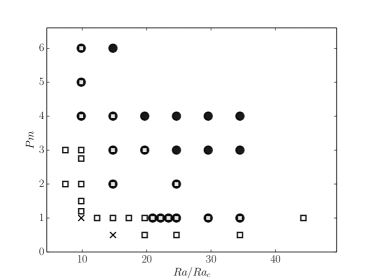
(a) (b)

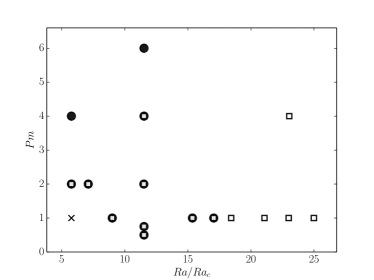
Figure 1: Dipolar (black circles) and multipolar (white squares) dynamos as a function of $Ra/Ra_{\text{c}}$ and $Pm$, for a central mass (a) and a uniform mass distribution (b). Crosses indicate the absence of a self-sustained dynamo.

In our simulations we recover the two distinct dynamo regimes observed with both Boussinesq (Kutzner & Christensen 2002; Christensen & Aubert 2006; Schrinner et al. 2012; Yadav et al. 2013a) and anelastic models (Gastine et al. 2012; Schrinner et al. 2014). These are characterized by different magnetic field configurations: dipolar dynamos are dominated by a strong axial dipole component, whereas “non-dipolar” dynamos usually present a more complex geometry with higher spatial and temporal variability. The branches are easily identified by continuing simulations performed with other parameters, for which the dipolar/multipolar characteristic was previously established. Figure 1(a) shows the regime diagram we obtained, as a function of the Rayleigh and magnetic Prandtl numbers. For comparison, we use the data from Schrinner et al. (2012) and show in Fig. 1(b) the same regime diagram obtained for Boussinesq models with a uniform mass distribution. For $Pm=1$, the transition from the dipolar to the multipolar branch can be triggered by an increase in $Ra$. In that case, the transition is due to the increasing role of inertia as revealed by $Ro_{\ell}$. Alternatively, the transition from multipolar to dipolar dynamo can be triggered by increasing $Pm$. Then, the multipolar branch is lost when the saturated amplitude of the mean zonal flow becomes too small to prevent the growth of the dipolar solution (see Schrinner et al. 2012). It is worth noting that the two branches overlap for a restricted parameter range for which dipolar and multipolar dynamos may coexist. In that case, the observed solution strongly depends of the initial magnetic field, so we tested both weak and strong field initial conditions for all our models to delimit the extent of the bi-stable zone with greater accuracy. Actually, multipolar dynamos are favoured by the stronger zonal wind that may develop with stress-free boundary conditions, allowing for this hysteretic transition (Schrinner et al. 2012). Finally, we see that the dynamo threshold is lower for multipolar models, which allows the multipolar branch to extend below the dipolar branch at low Rayleigh and magnetic Prandtl numbers. We see in Fig. 1(b) that this is different from Boussinesq models with a uniform mass distribution.

To investigate the different transitions between the different dynamo branches, we plot the Elsasser number $\Lambda=B^{2}_{\text{rms}}/(\Omega\varrho_{c}\mu\eta)$ in Fig. 2(a) (related to the Lorentz number by $\Lambda=Lo^{2}Pm/\text{E}$) as a function of the distance to the threshold for models at $Pm=1$ and $Pm=3$.

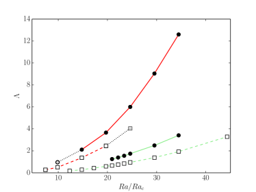
(a) (b)

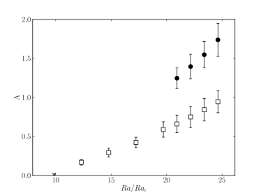
Figure 2: (a): Elsasser number $\Lambda$ as a function of $Ra/Ra_{\text{c}}$, for $Pm=1$ (green) and $Pm=3$ (red). The meaning of the symbol shapes is defined in the caption of Fig. 1. A grey marker indicates that the solution loses its stability. (b): Detail of the bifurcation close to the dynamo threshold for $Pm=1$. Error bars represent the standard deviations.

We see in Fig. 2(b) that the bifurcation for multipolar branch is supercritical. When decreasing the Rayleigh number, the dipolar branch loses its stability for $Ra/Ra_{\text{c}}\sim 20$, when the magnetic field strength becomes too weak.

For higher magnetic Prandtl numbers, the bifurcation of the multipolar branch still seems to be supercritical. Interestingly, one notes in Fig. 2(a) for $Pm=3$ that the multipolar branch loses its stability when increasing the Rayleigh number. A physical explanation for this behaviour is that the mean zonal flow does not grow fast enough as the field strength increases, and the dynamo switches to the dipolar solution. This simple physical scenario can be illustrated by comparing the variation in the field strength of the dipolar branch, as measured by $\Lambda^{\mathrm{dip}}$, and the zonal shear of the multipolar branch, as measured by $Ro_{z}^{\mathrm{mul}}$. Indeed, we see in Fig. 3 that the higher the magnetic Prandtl number, the faster the growth of the ratio between $\Lambda^{\mathrm{dip}}$ and $Ro_{z}^{\mathrm{mul}}$. This explains why the multipolar branch destabilizes at large forcing for larger $Pm$ ($Pm=3$, red dashed line in Fig. 2(a)), while it remains stable at smaller $Pm$ ($Pm=1$, green dashed line in Fig. 2(a)).

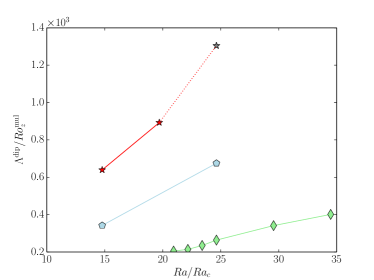
Figure 3: Ratio $\Lambda^{\mathrm{dip}}/Ro_{z}^{\mathrm{mul}}$ as a function of $Ra/Ra_{\text{c}}$, for $Pm=1$ (green diamonds), $Pm=2$ (blue pentagons) and $Pm=3$ (red stars). The point marked with the grey star has been computed with the model corresponding to the grey square in Fig. 2.

Because of computational limitations, we were not able to find for $Pm>1$ the Rayleigh numbers for which the dipolar branch should disappear.

3.2 Equatorial dipole

Schrinner et al. (2014) show that dipolar and multipolar dynamos in anelastic simulations were no longer distinguishable from each other in terms of $f_{\text{dip}}$, contrary to Boussinesq models. This smoother transition has been attributed to the presence of dynamos with a high equatorial dipole contribution, which leads to intermediate values for $f_{\text{dip}}$.

(a) (b)

Figure 4: (a): The relative dipole field strength $f_{\text{dip}}$ versus the local Rossby number. (b): The relative axial dipole field strength ${f_{\text{dip}}}_{\text{ax}}$ versus the local Rossby number. The meaning of the symbol shapes is defined in the caption of Fig. 1.

However, Fig. 4(a) shows that this tendency already exits at low $N_{\varrho}$, and thus cannot be accounted for only in terms of anelastic effects. Furthermore, when the equatorial dipole component is removed to compute the relative dipole field strength, we recover a more abrupt transition, as we can see in Fig. 4(b) which shows the relative axial dipole field strength ${f_{\text{dip}}}_{\text{ax}}$. Dipolar dynamos are left unchanged by this new definition, whereas multipolar dynamos of intermediate dipolarity are no longer observed, which confirms that the increase in $f_{\text{dip}}$ is due to a significant equatorial dipole component. The quantity ${f_{\text{dip}}}_{\text{ax}}$ therefore provides a robust criterion to distinguish the dipolar and the multipolar branches.

To further characterize the emergence of multipolar dynamos with a significant equatorial dipole contribution, we plot the values of the modified tilt angle $\theta$ in the parameter space in Fig. 5(a).

(a)

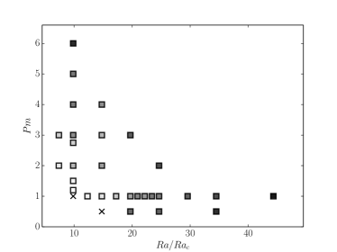
(b)

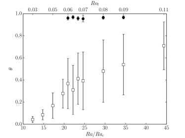
Figure 5: (a): Evolution of the modified tilt angle $\theta$ defined by Eq. (16) for multipolar dynamos as a function of $Ra/Ra_{\text{c}}$ and $Pm$. Colour scale ranges from white ($\theta=0$) to black ($\theta=0.7$). (b): $\theta$ as a function of $Ra/Ra_{\text{c}}$ for $Pm=1$. Upper $x$ axis corresponds to the values of $Ro_{\ell}$ for the multipolar branch. The meaning of the symbol shapes is defined in the caption of Fig. 1. Error bars represent the standard deviations.

Low values of $\theta$ are characteristic of an equatorial dipole on the surface of the outer sphere and they appear to be preferably localized close to the dynamo threshold of the multipolar branch, at low Rayleigh and magnetic Prandtl numbers. In our case, dynamos with a stronger equatorial dipole component belong to the class of multipolar dynamos, but since they are always close to the threshold, fewer modes are likely to be excited. As the Rayleigh number or the magnetic Prandtl number is increased, the dipole axis is not stable anymore but fluctuates in the interval $[0,\pi]$, which is typical of polarity reversals for multipolar dynamos (Kutzner & Christensen 2002). This evolution is illustrated in Fig. 5(b) for dynamos at $Pm=1$. For this subset of models, we computed the percentage of the non-axisymmetric magnetic energy density with respect to the total magnetic energy density $E_{\mathrm{m}}$ and saw that it tends to increase from 85% on average for multipolar dynamos up to 93% as the Rayleigh number is decreased.

Part of the changes reported in Schrinner et al. (2014) about anelastic dynamos simulations do not seem to come from the stratified reference density profile, but from the choice of a gravity profile proportional to $1/r^{2}$. This profile differs from the gravity profile proportional to $r$ that was used for Boussinesq simulations and is actually the only significant difference between previous studies and our low $N_{\varrho}$ simulations. As a consequence, convection cells form and stay closer to the inner sphere, as we can see in Fig. 6. We compare here equatorial cuts of the radial component of the velocity for both choices of gravity profile.

(a)

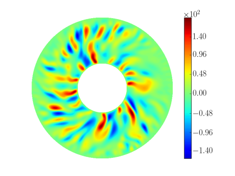
(b)

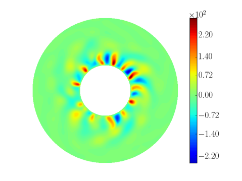
Figure 6: Equatorial cross section of the radial component of the velocity, with $E=10^{-4}$, $Pr=1$. (a): $g\propto r\,$ and $Ra/Ra_{\text{c}}=9.0\,$, $Pm=1$. (b): $g\propto 1/r^{2}$ and $Ra/Ra_{\text{c}}=9.9\,$, $Pm=1.2$.

This strong difference in the flow reflects on the localization of the active dynamo regions, as we can see in the corresponding cuts of the radial component of the magnetic field in Fig. 7.

(a)

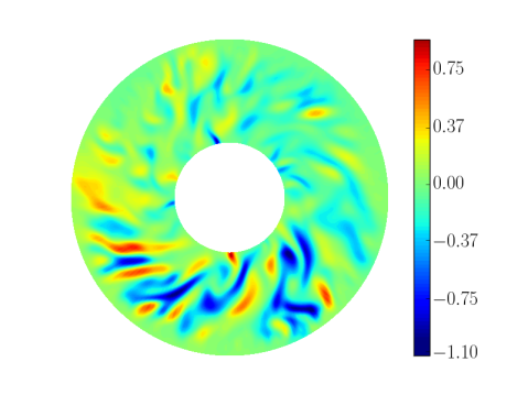
(b)

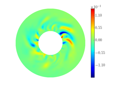
(c)

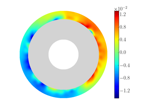
Figure 7: Equatorial cross section of the radial component of the magnetic field,with $E=10^{-4}$, $Pr=1$. (a): $g\propto r\,$ and $Ra/Ra_{\text{c}}=9.0\,$, $Pm=1$. (b),(c): $g\propto 1/r^{2}$ and $Ra/Ra_{\text{c}}=9.9\,$, $Pm=1.2$. Colour in figure (c) has been rescaled to highlight the emergence of a $m=1$ mode at the outer sphere.

With a gravity profile proportional to $1/r^{2}$, the magnetic field is mainly generated close to the inner sphere where the convection cells form. Consequently, our measure of the dipole field strength $f_{\text{dip}}$ at the surface of the outer sphere appears to be biased, since it will essentially be sensitive to the less diffusive large scale modes. This filter effect is likely to be responsible for the increase in $f_{\text{dip}}$ we reported in some anelastic dynamo models. However, for higher density stratification $N_{\varrho}=3$ and Prandtl numbers $Pr=2$ and $Pm=4$, Schrinner et al. (2014) identify equatorial dipole dynamos with a $m=1$ component that is not localized on the outer sphere and for which the present mechanism will not be relevant.

4 Conclusion

In this paper, we focussed on very weakly stratified anelastic dynamo models with a central mass distribution. We investigated the bifurcations between the dipolar and multipolar dynamo branches and recovered in parts the behaviour that has been observed for Boussinesq models with a uniform mass distribution. In addition, we show that the dipolar branch can now lose its stability and switch to the multipolar branch at low Rayleigh and magnetic Prandtl numbers. The multipolar dynamos that are observed in this restricted parameter regime usually present a stronger equatorial dipole component at the surface of the outer sphere. When increasing the Rayleigh number at higher $Pm$, it seems that the mean zonal flow does not grow fast enough to maintain the multipolar solution, and we identified several cases where the multipolar branch switches to the dipolar solution.

This study has shed interesting light on the recent systematic parameter study of spherical anelastic dynamo models started by Schrinner et al. (2014). Focussing on weakly stratified dynamo models, we showed that magnetic field configurations with a significant equatorial dipole contribution can already be observed in the Boussinesq limit. In the parameter regime we investigate, our study reveals that the choice of gravity profile has a strong influence on the fluid flow and thus on the dynamo generated magnetic field, depending whether one considers a uniform or a central mass distribution. In the parameter space, we showed that multipolar dynamos with a significant equatorial dipole contribution are preferably observed close to the dynamo threshold. This is reminiscent of the results of Aubert & Wicht (2004), who studied the competition between axial and equatorial dipolar dynamos when varying the aspect ratio of the spherical shell in geodynamo models.

However, the filter effect we highlight here focusses on the topology of the magnetic field at the outer surface of the models. As a consequence, it will not be able to explain the stronger equatorial dipole component for all models in Schrinner et al. (2014). Independently, Cole et al. (2014) also report the discovery of an azimuthal dynamo wave of a $m=1$ mode in numerical simulations corresponding to higher density stratification. Their Coriolis number plays a similar role to the inverse of our local Rossby number. Upper $x$ axis of Fig. 5(b) shows that equatorial dipole configurations are favoured with the decrease in $Ro_{\ell}$.

Observational results from photometry (Hackman et al. 2013) and spectropolarimetry (Kochukhov et al. 2013) of rapidly rotating cool active stars reveal that the surface magnetic field of these objects can be highly non-axisymmetric. Further investigation of direct numerical simulations is therefore required to better understand the influence of the Prandtl number and the density stratification on the magnetic field topology.

Appendix A Scaling laws

For our samples of models we compute the usual scaling laws that have been derived for the magnetic and velocity fields and the convective heat flux (Christensen & Aubert 2006; Yadav et al. 2013a; Stelzer & Jackson 2013; Yadav et al. 2013b). As in Schrinner et al. (2014), we do not attempt to solve any secondary dependence on $Pm$ because we do not vary this parameter on a wide enough range. We transform our problem to a linear one by taking the logarithm and look for a law of the form $\ln\hat{y}=\beta+\alpha\ln x$. To quantify the misfit between data and fitted values, we follow Christensen & Aubert (2006) and compute the relative misfit

$$\chi_{rel}=\sqrt{\frac{1}{n}\sum_{i=1}^{n}\left(\frac{y_{i}-\hat{y_{i}}}{y_{i}}\right)^{2}}\,,$$ (17)

where $\hat{y_{i}}$ stands for predicted values, $y_{i}$ for measured values, and $n$ is the number of data. Our results are summarized in Table 1 and compared with those found in Schrinner et al. (2014) and Yadav et al. (2013a) in Table 2. We did not find significant differences between the anelastic scalings and the scaling we obtained in the Boussinesq limit with the same mass distribution. The coefficients we obtained seem closer on average to the coefficients obtained by Yadav et al. (2013a) with Boussinesq models with a uniform mass distribution. However, it is not possible to deduce from our data set any influence of $N_{\varrho}$ on the different coefficients of the scaling laws. In our models, the Nusselt number evaluated at the surface of the inner sphere $S_{\!i}$ is defined by

$$Nu_{\mathrm{bot}}=-\frac{(\exp{(N_{\varrho})}-1)w_{i}r_{i}^{2}}{4\pi nc_{1}}\int_{S_{\!i}}\frac{\partial s}{\partial r}\sin\theta\mathop{}\!\mathrm{d}\theta\mathop{}\!\mathrm{d}\phi\,,$$ (18)

which enables a flux based Rayleigh number to be defined,

$$Ra_{Q}=Nu^{\star}\,\frac{Ra\,E^{2}}{r_{\!o}^{2}\,Pr}\quad\text{with}\quad Nu^{\star}=(Nu_{\mathrm{bot}}-1)\,\frac{E}{Pr}\,,$$ (19)

which is used in derivating scaling laws, together with the fraction of ohmic to total dissipation $f_{\text{ohm}}$.

Table 1: Summary of the coefficients obtained for the different scaling laws, with their standard error from the linear regression.

Scaling	$\alpha$	$\beta$	$\chi_{rel}$
$Lo/\sqrt{f_{\text{ohm}}}$
multipolar	$0.29\pm 0.01$	$-0.52\pm 0.1$	$0.06$
dipolar	$0.32\pm 0.02$	$-0.08\pm 0.2$	$0.06$
$Ro$	$0.39\pm 0.01$	$0.35\pm 0.2$	$0.1$
$Nu^{\star}$	$0.58\pm 0.003$	$-1.16\pm 0.04$	$0.03$

Table 2: Comparison between the different scaling laws obtained with different dynamo models. RPD refers to the present study, SPRD to Schrinner et al. (2014), and YGC to Yadav et al. (2013a), respectively.

Scaling	RPD		SPRD		YGC
	c	x	c	x	c	x
$g$	$1/r^{2}$		$1/r^{2}$		$r$
$N_{\varrho}$	$\leq 0.1$		$\in\left[0.5,4\right]$		$0$
$Lo/\sqrt{f_{\text{ohm}}}=c\,Ra_{Q}^{x}$
multipolar	0.59	0.29	1.19	0.34	0.65	0.35
dipolar	0.92	0.32	1.58	0.35	1.08	0.37
$Ro=c\,Ra_{Q}^{x}$	1.42	0.39	1.66	0.42	1.79	0.44
					0.73	0.39
$Nu^{\star}=c\,Ra_{Q}^{x}$	0.31	0.58	0.25	0.59	0.06	0.52

Appendix B Numerical models

Table 3: Overview of the simulations carried out with $E=10^{-4}$, $Pr=1$, $\chi=0.35$, $n=2$, and $N_{\varrho}=0.1$.

Model	$Ra$	$Pm$	$Ro$	$Ro_{\ell}$	$\ell_{c}$	$Lo$	$Nu$	$f_{\text{dip}}$	${f_{\text{dip}}}_{\text{ax}}$	$f_{\text{ohm}}$
$1\mathrm{m}$	$1.50\times 10^{6}$	$2.00$	$3.6\times 10^{-3}$	$2.0\times 10^{-2}$	$1.8\times 10^{1}$	$2.1\times 10^{-3}$	$1.4$	$4.9\times 10^{-1}$	$8.0\times 10^{-2}$	$8.0\times 10^{-2}$
$2\mathrm{m}$	$1.50\times 10^{6}$	$3.00$	$3.8\times 10^{-3}$	$2.0\times 10^{-2}$	$1.6\times 10^{1}$	$3.0\times 10^{-3}$	$1.5$	$3.2\times 10^{-1}$	$9.5\times 10^{-2}$	$1.5\times 10^{-1}$
$3\mathrm{m}$	$2.00\times 10^{6}$	$1.20$	$6.8\times 10^{-3}$	$2.6\times 10^{-2}$	$1.7\times 10^{1}$	$2.5\times 10^{-3}$	$1.7$	$6.7\times 10^{-1}$	$2.7\times 10^{-2}$	$8.1\times 10^{-2}$
$4\mathrm{m}$	$2.00\times 10^{6}$	$1.50$	$6.2\times 10^{-3}$	$2.7\times 10^{-2}$	$1.7\times 10^{1}$	$3.1\times 10^{-3}$	$1.7$	$5.7\times 10^{-1}$	$4.3\times 10^{-2}$	$1.3\times 10^{-1}$
$5\mathrm{m}$	$2.00\times 10^{6}$	$2.00$	$5.1\times 10^{-3}$	$2.7\times 10^{-2}$	$1.7\times 10^{1}$	$3.6\times 10^{-3}$	$1.8$	$5.2\times 10^{-1}$	$2.5\times 10^{-1}$	$1.7\times 10^{-1}$
$6\mathrm{m}$	$2.00\times 10^{6}$	$2.75$	$5.2\times 10^{-3}$	$2.8\times 10^{-2}$	$1.7\times 10^{1}$	$4.0\times 10^{-3}$	$1.8$	$3.0\times 10^{-1}$	$8.0\times 10^{-3}$	$2.1\times 10^{-1}$
$7\mathrm{m}$	$2.00\times 10^{6}$	$2.90$	$5.2\times 10^{-3}$	$2.3\times 10^{-2}$	$1.6\times 10^{1}$	$4.1\times 10^{-3}$	$1.8$	$6.4\times 10^{-1}$	$1.3\times 10^{-1}$	$1.9\times 10^{-1}$
$8\mathrm{m}$	$2.00\times 10^{6}$	$3.00$	$5.9\times 10^{-3}$	$2.6\times 10^{-2}$	$1.6\times 10^{1}$	$4.1\times 10^{-3}$	$1.8$	$3.7\times 10^{-1}$	$2.4\times 10^{-1}$	$1.9\times 10^{-1}$
$9\mathrm{m}$	$2.00\times 10^{6}$	$4.00$	$5.6\times 10^{-3}$	$2.6\times 10^{-2}$	$1.6\times 10^{1}$	$4.5\times 10^{-3}$	$1.8$	$3.0\times 10^{-1}$	$2.1\times 10^{-1}$	$2.2\times 10^{-1}$
$9\mathrm{d}$	$2.00\times 10^{6}$	$4.00$	$5.3\times 10^{-3}$	$2.2\times 10^{-2}$	$1.4\times 10^{1}$	$6.6\times 10^{-3}$	$1.7$	$8.2\times 10^{-1}$	$8.2\times 10^{-1}$	$4.0\times 10^{-1}$
$10\mathrm{m}$	$2.00\times 10^{6}$	$5.00$	$5.5\times 10^{-3}$	$2.6\times 10^{-2}$	$1.6\times 10^{1}$	$4.7\times 10^{-3}$	$1.8$	$3.4\times 10^{-1}$	$2.5\times 10^{-1}$	$2.3\times 10^{-1}$
$10\mathrm{d}$	$2.00\times 10^{6}$	$5.00$	$5.3\times 10^{-3}$	$2.6\times 10^{-2}$	$1.4\times 10^{1}$	$6.6\times 10^{-3}$	$1.8$	$8.4\times 10^{-1}$	$8.4\times 10^{-1}$	$3.9\times 10^{-1}$
$11\mathrm{m}$	$2.00\times 10^{6}$	$6.00$	$5.4\times 10^{-3}$	$2.6\times 10^{-2}$	$1.6\times 10^{1}$	$4.8\times 10^{-3}$	$1.8$	$3.4\times 10^{-1}$	$3.1\times 10^{-1}$	$2.5\times 10^{-1}$
$11\mathrm{d}$	$2.00\times 10^{6}$	$6.00$	$5.7\times 10^{-3}$	$2.2\times 10^{-2}$	$1.3\times 10^{1}$	$9.0\times 10^{-3}$	$1.9$	$6.7\times 10^{-1}$	$6.7\times 10^{-1}$	$4.9\times 10^{-1}$
$12\mathrm{m}$	$2.50\times 10^{6}$	$1.00$	$8.0\times 10^{-3}$	$3.3\times 10^{-2}$	$1.6\times 10^{1}$	$4.1\times 10^{-3}$	$2.0$	$6.5\times 10^{-1}$	$6.0\times 10^{-2}$	$1.8\times 10^{-1}$
$13\mathrm{m}$	$3.00\times 10^{6}$	$1.00$	$7.8\times 10^{-3}$	$4.0\times 10^{-2}$	$1.6\times 10^{1}$	$5.3\times 10^{-3}$	$2.3$	$5.8\times 10^{-1}$	$1.0\times 10^{-1}$	$2.2\times 10^{-1}$
$14\mathrm{m}$	$3.00\times 10^{6}$	$2.00$	$8.9\times 10^{-3}$	$4.0\times 10^{-2}$	$1.6\times 10^{1}$	$6.4\times 10^{-3}$	$2.4$	$3.6\times 10^{-1}$	$2.1\times 10^{-1}$	$2.6\times 10^{-1}$
$14\mathrm{d}$	$3.00\times 10^{6}$	$2.00$	$7.4\times 10^{-3}$	$3.7\times 10^{-2}$	$1.5\times 10^{1}$	$8.1\times 10^{-3}$	$2.4$	$8.3\times 10^{-1}$	$7.9\times 10^{-1}$	$3.9\times 10^{-1}$
$15\mathrm{m}$	$3.00\times 10^{6}$	$3.00$	$8.7\times 10^{-3}$	$4.0\times 10^{-2}$	$1.6\times 10^{1}$	$6.8\times 10^{-3}$	$2.5$	$2.9\times 10^{-1}$	$1.3\times 10^{-1}$	$2.8\times 10^{-1}$
$15\mathrm{d}$	$3.00\times 10^{6}$	$3.00$	$7.5\times 10^{-3}$	$3.7\times 10^{-2}$	$1.6\times 10^{1}$	$8.4\times 10^{-3}$	$2.3$	$7.8\times 10^{-1}$	$7.7\times 10^{-1}$	$4.0\times 10^{-1}$
$16\mathrm{m}$	$3.00\times 10^{6}$	$4.00$	$8.2\times 10^{-3}$	$3.9\times 10^{-2}$	$1.6\times 10^{1}$	$7.2\times 10^{-3}$	$2.4$	$2.8\times 10^{-1}$	$1.8\times 10^{-1}$	$3.1\times 10^{-1}$
$16\mathrm{d}$	$3.00\times 10^{6}$	$4.00$	$7.5\times 10^{-3}$	$3.7\times 10^{-2}$	$1.6\times 10^{1}$	$8.7\times 10^{-3}$	$2.4$	$7.3\times 10^{-1}$	$7.2\times 10^{-1}$	$4.0\times 10^{-1}$
$17\mathrm{d}$	$3.00\times 10^{6}$	$6.00$	$7.8\times 10^{-3}$	$3.7\times 10^{-2}$	$1.5\times 10^{1}$	$9.2\times 10^{-3}$	$2.5$	$7.3\times 10^{-1}$	$7.3\times 10^{-1}$	$4.0\times 10^{-1}$
$18\mathrm{m}$	$3.50\times 10^{6}$	$1.00$	$9.1\times 10^{-3}$	$4.6\times 10^{-2}$	$1.6\times 10^{1}$	$6.5\times 10^{-3}$	$2.6$	$5.0\times 10^{-1}$	$1.8\times 10^{-1}$	$2.5\times 10^{-1}$
$19\mathrm{m}$	$4.00\times 10^{6}$	$0.50$	$1.7\times 10^{-2}$	$4.8\times 10^{-2}$	$1.6\times 10^{1}$	$4.9\times 10^{-3}$	$2.7$	$1.9\times 10^{-1}$	$1.3\times 10^{-1}$	$1.9\times 10^{-1}$
$20\mathrm{m}$	$4.00\times 10^{6}$	$1.00$	$1.0\times 10^{-2}$	$5.3\times 10^{-2}$	$1.6\times 10^{1}$	$7.7\times 10^{-3}$	$3.0$	$5.0\times 10^{-1}$	$2.2\times 10^{-1}$	$3.1\times 10^{-1}$
$21\mathrm{m}$	$4.00\times 10^{6}$	$3.00$	$1.1\times 10^{-2}$	$5.2\times 10^{-2}$	$1.6\times 10^{1}$	$9.0\times 10^{-3}$	$3.1$	$3.0\times 10^{-1}$	$2.4\times 10^{-1}$	$3.4\times 10^{-1}$
$21\mathrm{d}$	$4.00\times 10^{6}$	$3.00$	$1.0\times 10^{-2}$	$4.9\times 10^{-2}$	$1.6\times 10^{1}$	$1.1\times 10^{-2}$	$3.1$	$6.5\times 10^{-1}$	$6.5\times 10^{-1}$	$4.2\times 10^{-1}$
$22\mathrm{d}$	$4.00\times 10^{6}$	$4.00$	$1.0\times 10^{-2}$	$4.9\times 10^{-2}$	$1.5\times 10^{1}$	$1.2\times 10^{-2}$	$3.1$	$6.6\times 10^{-1}$	$6.5\times 10^{-1}$	$4.3\times 10^{-1}$
$23\mathrm{m}$	$4.25\times 10^{6}$	$1.00$	$1.1\times 10^{-2}$	$5.7\times 10^{-2}$	$1.6\times 10^{1}$	$8.1\times 10^{-3}$	$3.2$	$4.0\times 10^{-1}$	$2.6\times 10^{-1}$	$2.8\times 10^{-1}$
$23\mathrm{d}$	$4.25\times 10^{6}$	$1.00$	$1.0\times 10^{-2}$	$5.1\times 10^{-2}$	$1.6\times 10^{1}$	$1.1\times 10^{-2}$	$3.2$	$9.4\times 10^{-1}$	$9.4\times 10^{-1}$	$4.4\times 10^{-1}$
$24\mathrm{m}$	$4.50\times 10^{6}$	$1.00$	$1.2\times 10^{-2}$	$6.0\times 10^{-2}$	$1.6\times 10^{1}$	$8.7\times 10^{-3}$	$3.4$	$3.4\times 10^{-1}$	$1.1\times 10^{-1}$	$3.0\times 10^{-1}$
$24\mathrm{d}$	$4.50\times 10^{6}$	$1.00$	$1.1\times 10^{-2}$	$5.5\times 10^{-2}$	$1.6\times 10^{1}$	$1.2\times 10^{-2}$	$3.4$	$9.3\times 10^{-1}$	$9.3\times 10^{-1}$	$4.4\times 10^{-1}$
$25\mathrm{m}$	$4.75\times 10^{6}$	$1.00$	$1.2\times 10^{-2}$	$6.2\times 10^{-2}$	$1.6\times 10^{1}$	$9.2\times 10^{-3}$	$3.6$	$3.5\times 10^{-1}$	$2.7\times 10^{-1}$	$3.0\times 10^{-1}$
$25\mathrm{d}$	$4.75\times 10^{6}$	$1.00$	$1.2\times 10^{-2}$	$5.7\times 10^{-2}$	$1.5\times 10^{1}$	$1.2\times 10^{-2}$	$3.6$	$9.2\times 10^{-1}$	$9.2\times 10^{-1}$	$4.5\times 10^{-1}$
$26\mathrm{m}$	$5.00\times 10^{6}$	$0.50$	$1.7\times 10^{-2}$	$6.6\times 10^{-2}$	$1.6\times 10^{1}$	$8.1\times 10^{-3}$	$3.7$	$2.9\times 10^{-1}$	$2.0\times 10^{-1}$	$2.5\times 10^{-1}$
$27\mathrm{m}$	$5.00\times 10^{6}$	$1.00$	$1.3\times 10^{-2}$	$6.6\times 10^{-2}$	$1.6\times 10^{1}$	$9.7\times 10^{-3}$	$3.8$	$3.7\times 10^{-1}$	$2.3\times 10^{-1}$	$3.2\times 10^{-1}$
$28\mathrm{d}$	$5.00\times 10^{6}$	$1.00$	$1.2\times 10^{-2}$	$6.0\times 10^{-2}$	$1.5\times 10^{1}$	$1.3\times 10^{-2}$	$3.8$	$9.2\times 10^{-1}$	$9.2\times 10^{-1}$	$4.6\times 10^{-1}$
$29\mathrm{m}$	$5.00\times 10^{6}$	$2.00$	$1.4\times 10^{-2}$	$6.7\times 10^{-2}$	$1.6\times 10^{1}$	$1.1\times 10^{-2}$	$3.9$	$2.5\times 10^{-1}$	$2.1\times 10^{-1}$	$3.6\times 10^{-1}$
$30\mathrm{d}$	$5.00\times 10^{6}$	$2.00$	$1.2\times 10^{-2}$	$6.1\times 10^{-2}$	$1.6\times 10^{1}$	$1.4\times 10^{-2}$	$3.9$	$7.2\times 10^{-1}$	$7.2\times 10^{-1}$	$4.6\times 10^{-1}$
$31\mathrm{d}$	$5.00\times 10^{6}$	$3.00$	$1.2\times 10^{-2}$	$6.1\times 10^{-2}$	$1.6\times 10^{1}$	$1.4\times 10^{-2}$	$3.9$	$6.4\times 10^{-1}$	$6.3\times 10^{-1}$	$4.6\times 10^{-1}$
$32\mathrm{d}$	$5.00\times 10^{6}$	$4.00$	$1.3\times 10^{-2}$	$6.2\times 10^{-2}$	$1.6\times 10^{1}$	$1.4\times 10^{-2}$	$4.1$	$7.3\times 10^{-1}$	$7.3\times 10^{-1}$	$4.3\times 10^{-1}$
$33\mathrm{m}$	$6.00\times 10^{6}$	$1.00$	$1.5\times 10^{-2}$	$7.8\times 10^{-2}$	$1.6\times 10^{1}$	$1.2\times 10^{-2}$	$4.5$	$3.5\times 10^{-1}$	$2.9\times 10^{-1}$	$3.4\times 10^{-1}$
$34\mathrm{d}$	$6.00\times 10^{6}$	$1.00$	$1.5\times 10^{-2}$	$7.2\times 10^{-2}$	$1.5\times 10^{1}$	$1.6\times 10^{-2}$	$4.6$	$9.1\times 10^{-1}$	$9.1\times 10^{-1}$	$4.9\times 10^{-1}$
$35\mathrm{d}$	$6.00\times 10^{6}$	$3.00$	$1.4\times 10^{-2}$	$7.1\times 10^{-2}$	$1.6\times 10^{1}$	$1.7\times 10^{-2}$	$4.7$	$6.8\times 10^{-1}$	$6.8\times 10^{-1}$	$4.8\times 10^{-1}$
$36\mathrm{d}$	$6.00\times 10^{6}$	$4.00$	$1.5\times 10^{-2}$	$7.4\times 10^{-2}$	$1.6\times 10^{1}$	$1.8\times 10^{-2}$	$4.9$	$7.2\times 10^{-1}$	$7.2\times 10^{-1}$	$4.7\times 10^{-1}$
$37\mathrm{m}$	$7.00\times 10^{6}$	$0.50$	$1.8\times 10^{-2}$	$9.2\times 10^{-2}$	$1.6\times 10^{1}$	$1.2\times 10^{-2}$	$5.2$	$2.4\times 10^{-1}$	$2.1\times 10^{-1}$	$3.7\times 10^{-1}$
$38\mathrm{m}$	$7.00\times 10^{6}$	$1.00$	$2.0\times 10^{-2}$	$9.3\times 10^{-2}$	$1.6\times 10^{1}$	$1.4\times 10^{-2}$	$5.5$	$2.9\times 10^{-1}$	$2.5\times 10^{-1}$	$3.7\times 10^{-1}$
$38\mathrm{d}$	$7.00\times 10^{6}$	$1.00$	$1.7\times 10^{-2}$	$8.0\times 10^{-2}$	$1.5\times 10^{1}$	$1.8\times 10^{-2}$	$5.2$	$8.9\times 10^{-1}$	$8.9\times 10^{-1}$	$5.2\times 10^{-1}$
$39\mathrm{d}$	$7.00\times 10^{6}$	$3.00$	$1.6\times 10^{-2}$	$7.7\times 10^{-2}$	$1.5\times 10^{1}$	$2.0\times 10^{-2}$	$5.4$	$7.2\times 10^{-1}$	$7.2\times 10^{-1}$	$5.2\times 10^{-1}$
$40\mathrm{d}$	$7.00\times 10^{6}$	$4.00$	$1.7\times 10^{-2}$	$8.0\times 10^{-2}$	$1.6\times 10^{1}$	$2.1\times 10^{-2}$	$5.4$	$8.4\times 10^{-1}$	$8.4\times 10^{-1}$	$5.0\times 10^{-1}$
$41\mathrm{m}$	$9.00\times 10^{6}$	$1.00$	$2.4\times 10^{-2}$	$1.1\times 10^{-1}$	$1.5\times 10^{1}$	$1.8\times 10^{-2}$	$6.8$	$3.5\times 10^{-1}$	$3.3\times 10^{-1}$	$4.1\times 10^{-1}$

Table 3: (continued)