Damping of glacial-interglacial cycles from anthropogenic forcing

Abstract

Climate variability over the past million years shows a strong glacial-interglacial cycle of $\sim$100,000 years as a combined result of Milankovitch orbital forcing and climatic resonance. It has been suggested that anthropogenic contributions to radiative forcing may extend the length of the present interglacial, but the effects of anthropogenic forcing on the periodicity of glacial-interglacial cycles has received little attention. Here I demonstrate that moderate anthropogenic forcing can act to damp this 100,000 year cycle and reduce climate variability from orbital forcing. Future changes in solar insolation alone will continue to drive a 100,000 year climate cycle over the next million years, but the presence of anthropogenic warming can force the climate into an ice-free state that only weakly responds to orbital forcing. Sufficiently strong anthropogenic forcing that eliminates the glacial-interglacial cycle may serve as an indication of an epoch transition from the Pleistocene to the Anthropocene.

Gindraft=false HAQQ-MISRA DAMPING OF GLACIAL CYCLES Corresponding author: J. Haqq-Misra, Blue Marble Space Institute of Science, 1200 Westlake Ave N Suite 1006, Seattle, Washington 98109, USA. (jacob@bmsis.org)

1 Introduction

Long-term patterns of global temperature derived from ice cores (Petit et al., 1999; Jouzel et al., 2007) and deep-sea oxygen isotopes (Shackleton, 2000) indicate cycles in the extent of global ice coverage with periods of 100,000, 41,000, and 23,000 years as the dominant signals (Hays et al., 1976; Imbrie et al., 1993). The 41,000 and 23,000 year signals correlate directly with changes in solar insolation from variations in obliquity and orbital precession; however, the corresponding changes in insolation from eccentricity variation on a 100,000 year timescale are too weak to drive the glacial-interglacial features observed in the geologic record (Watts and Hayder, 1984; Genthon et al., 1987; Imbrie et al., 1993; Rutherford and D’Hondt, 2000; Loulergue et al., 2008).

A possible explanation for this discrepancy between eccentricity forcing strength and glacial cycles is that internal climate mechanisms amplify changes in insolation to yield a strong $\sim$100,000 year glacial-interglacial cycle. Climatic resonances may occur from a combination of mechanisms, such as the thermal inertia of oceans and large ice sheets (Watts and Hayder, 1984; Imbrie et al., 1993) or long-term cycles in carbon dioxide and methane (Genthon et al., 1987; Loulergue et al., 2008), but these complex feedback patterns are difficult to simulate with climate models over million year timescales.

It has been suggested that anthropogenic forcing may delay the onset of the next glacial period (Mitchell, 1972; Loutre and Berger, 2000), but the long-term effect on the periodicity of this cycle has received little attention. Here a stochastic energy balance model (EBM) is used to demonstrate that anthropogenic forcing can damp this glacial-interglacial cycle. This EBM is tuned to a state of stochastic resonance that experiences variations in global average temperature with a 100,000 year period. This periodic signal is damped with sufficiently strong anthropogenic forcing, which suggests the possibility that glacial-interglacial cycles could cease in the future.

2 Small ice cap instability

Simple climate models have been used to argue that ice caps can only grow to $\sim$30^∘ latitude, beyond which the planet falls into a completely ice-covered state (North et al., 1981; Caldeira and Kasting, 1992). These models also exhibit a small ice cap instability that result in the complete loss of an ice cap when it shrinks to a critical size (North, 1984). The small ice instability is of relevance to the 100,000 year glacial-interglacial cycle because it allows for multiple equilibrium solutions for present-day values of relative solar flux, which suggests that long-term orbital forcing could drive climate to cycle between glacial and ice-free conditions.

For this study, a one-dimensional energy balance model (Fairén et al., 2012) is modified to calculate meridionally averaged temperature profiles $T$ as a function of latitude $\theta$ and time $t$ according to the equation

$$C\frac{\partial T(\theta,t)}{\partial t}=\bar{S}(\theta,L)\left(1-\alpha(T)\right)-\left(A+BT(\theta,t)\right)\\ +\frac{1}{\cos\theta}\frac{\partial}{\partial\theta}\left(D\cos\theta\frac{\partial T(\theta,t)}{\partial\theta}\right),$$ (1)

where $C$ is effective heat capacity of the surface and atmosphere, $\bar{S}$ is diurnally-averaged solar flux, $\alpha$ is top-of-atmosphere albedo, $A$ and $B$ are infrared flux constants, and $D$ is a diffusive parameter to describe the efficiency of meridional energy transport. Diurnally-averaged solar flux $\bar{S}=Sf(\theta,L)$ is the product of a constant solar flux $S$ and a function of latitude $\theta$ and orbital longitude $L(t,e,{\delta}_{0},L_{p})$, which depends on present-day values of eccentricity $e$, obliquity ${\delta}_{0}$, and the longitude of perihelion $L_{p}$, to yield seasonally-varying insolation (Gaidos and Williams, 2004). Uniform geography is assumed with constant heat capacity $C=2.1\times 10^{8}$ J m^-2 K^-1 to simulate an aquaplanet. Albedo is defined as $\alpha=0.291$ for $T\geq 263.15$ and $\alpha=0.663$ for $T<263.15$ (note that the precision of these albedo values reflects the tuning of the model (Caldeira and Kasting, 1992; Gaidos and Williams, 2004).) The parameter $D$ is set to a fixed value $D=0.38$ W m^-2 K^-1 that allows the model to reproduce present-day Earth conditions (Gaidos and Williams, 2004). Outgoing infrared flux is parameterized as a linear function of temperature with constants $A=203.3$ W m^-2 and $B=2.09$ W m^{-2 ∘}C^-1 tuned to present-day Earth (North et al., 1981). The model is discretized into 18 equally spaced latitudinal zones with an initial temperature profile $T(\theta,0)=T_{0}(\theta)$ and stepped through $\tau$ complete orbits by increments of ${\Delta}t=8.64\times 10^{3}$ s to numerically solve Eq. (1).

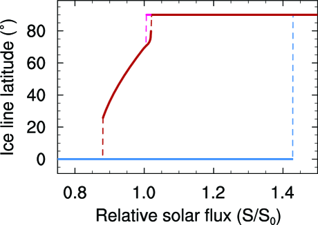
Figure 1: Energy balance model for the climate of Earth. Equilibrium climate states are calculated by initializing a deterministic energy balance model from present-day (red), ice-free (pink), and ice-covered (blue) conditions. Dotted lines show discontinuous transitions between climate states, including a maximum ice line of ${\sim}25^{\circ}$ and a deglaciation threshold of $S/S_{0}>1.4$. A “small ice cap instability” is evident as discrete transitions between ice-free and ice-cap states (dashed red and pink lines near $S/S_{0}=1$), which permits multiple equilibrium solutions for certain values of $S/S_{0}$.

This model behavior is shown in Fig. 1, which gives the equilibrium ice line latitude as a function of relative solar flux. These equilibrium climate states are calculated by initializing the EBM with present-day Earth ($T_{0}(|\theta|>70^{\circ})<263.16$ K and $T_{0}(|\theta|<70^{\circ})>263.16$ K, red curve), ice-free ($T_{0}(\theta)>273.16$ K, pink curve), and ice-covered ($T_{0}(\theta)=233$ K, blue curve) conditions for each value of relative solar flux $S/S_{0}$ (where $S_{0}=1360$ W m^-2). The EBM is iterated for $\tau=100$ model years in increments of ${\Delta}\tau=1$ yr to reach a statistically steady-state (where ${\delta}T/{\delta}t{\approx}0$) and find the extent of the ice line latitude ${\theta}_{i}$ (where $T({\theta}_{i})=263.16$ K). This results in two hysteresis loops: one between ice-covered and ice-free states (from ${\sim}0.85<S/S_{0}<{\sim}1.45$) and another between small ice cap and ice-free states (near $S/S_{0}{\sim}1.0$). This second loop is the small ice cap instability that describes transitions between glacial and ice-free conditions.

This simplified model is designed to highlight the multiple equilibria that can exist for Earth-like climates. Ice cap instabilities are well-known features of EBMs (North et al., 1981; North, 1984), and more recent studies with global climate models (GCMs) have shown some success in demonstrating a maximum ice line latitude and a large ice cap instability (DeConto and Pollard, 2003; Ishiwatari et al., 2007). The small ice cap instability has also been observed in GCM simulations (Lee and North, 1995; Winton, 2006), although it is not yet clear why this feature is present in some GCMs but not others. With this in mind, the use of an EBM in the analysis that follows is intended to be a qualitative approach to a problem that eventually could be approached with more sophisticated tools.

3 Stochastic resonance

The concept of stochastic resonance suggests that small random fluctuations in temperature are amplified by non-linear responses in the climate system, which establishes periodic transitions between glacial and ice-free conditions when orbital forcing is applied (Benzi et al., 1982; Imkeller, 2001). These random fluctuations represent the cumulative effect of any climatic resonance mechanisms present in the Earth system and allow for an abstracted implementation of resonance in climate models. A climate model in a state of stochastic resonance, when driven by Milankovitch orbital forcing, will show a 100,000 year periodicity in the global extent of glacial ice (ranging from large ice caps to ice-free conditions) associated with a change in global average temperature (spanning a range of ${\sim}10$ K), in addition to the shorter glacial cycles.

Figure 2: Histogram of estimated values for the noise parameter $\varepsilon$. This distribution includes 100 values with mean 0.334 W² m^-4 and standard deviation 0.07 W² m^-4.

A stochastic EBM is developed by modifying Eq. (1) to include a randomly fluctuating term, so that

$$C\frac{\partial T(\theta,t)}{\partial t}=\bar{S}(\theta,L)\left(1-\alpha(T)\right)-\left(A+BT(\theta,t)\right)\\ +\frac{1}{\cos\theta}\frac{\partial}{\partial\theta}\left(D\cos\theta\frac{\partial T(\theta,t)}{\partial\theta}\right)+\sqrt{\varepsilon}\dot{W},$$ (2)

where $\varepsilon$ is a tunable constant known as the ”noise parameter”, and $\dot{W}$ represents Gaussian white noise with zero expectation and unit variance. Eq. (2) represents a stochastic EBM when $\varepsilon>0$ and reduces to a deterministic EBM (Eq. (1)) when $\varepsilon=0$.

The constant $\varepsilon$ in Eq. (2) is optimized to find a state of stochastic resonance (Benzi et al., 1982; Imkeller, 2001) so that the EBM exhibits periodic transitions between warm and cool climates while avoiding global glaciation. Variations in mean annual insolation between -1 Myr and +1 Myr from the present are obtained from orbital and precessional calculations (Laskar et al., 2004) that yield time-dependent quantities for solar flux $S(\tau)$, eccentricity $e(\tau)$, obliquity $\delta_{0}(\tau)$, and the longitude of perihelion $L_{p}(\tau)$. This allows the stochastic EBM to iterate for $\tau=2$ million model years in increments of ${\Delta}\tau=1000$ years to simulate periodic variability of past and future climate. An optimal choice of $\varepsilon$ will exhibit glacial cycles near the 100,000, 41,000, and 23,000 yr periods that result from orbital and precessional forcing (Imbrie et al., 1993), whereas this feature of stochastic resonance will be lost if $\varepsilon$ is too small or too large (Benzi et al., 1982; Imkeller, 2001).

An appropriate choice for $\varepsilon$ is a value that maximizes a power spectrum (or periodogram) at a 100,000 yr period. A golden section search algorithm is applied to the stochastic EBM to identify a value of $\varepsilon$ that yields a power spectrum with a maximum value closest to 100,000 yr. This optimization algorithm is initialized with a search interval for $\varepsilon$ between 0.1 and 0.5 W² m^-4, and two sets of 2 Myr stochastic EBM calculations are performed with two different values of $\varepsilon$ within this range. The power spectrum of each of these model calculations is evaluated at a period of 100,000 yr, and the calculation that gives a larger value of this 100,000 yr power spectrum signal is retained for further optimization. Iteration continues until an optimal value of $\varepsilon$ is reached with a tolerance of 0.001 W² m^-4. Following a sample average approximation method (Kleywegt et al., 2001), this optimization process is repeated 100 times, and the resulting set of 100 estimated values is shown as a histogram in Fig. 2. The average of this distribution of gives an expected optimal value of $\varepsilon=0.334$ W² m^-4 with a standard deviation of 0.07 W² m^-4.

This tuned stochastic EBM is driven by Milankovitch orbital forcing (Laskar et al., 2004) to calculate global average temperature from -1 Myr to +1 Myr in the absence of any anthropogenic forcing. A 100-member control ensemble of 2 Myr stochastic EBM calculations (with $\varepsilon$ set to the expected optimal value) is calculated to give an expectation of global temperature evolution, and Fig. 3 (top panel) shows the full 100-member ensemble mean (black curve), a 10-member ensemble mean (blue curve), and the range of ensemble members (gray shading). The system is in stochastic resonance between climates warmer and cooler than today and manages to avoid global ice-covered or permanent ice-free states that would halt this periodicity.

An expected power spectrum of this 100-member control ensemble is shown in Fig. 4 (left panel). The full 100-member ensemble (black curve) shows its strongest peaks at $\sim$100,000 to $\sim$180,000 yr, which coincides approximately with the strongest signal of climate variability observed during the past 1 Myr. The 10-member ensemble subset (blue curve) has a more pronounced signal at 400,000 yr, although a peak near a $\sim$100,000 yr period is still evident, and the range of ensemble members (gray shading) indicates peaks at both $\sim$200,000 and $\sim$400,000 yr. (Note that all curves in the left panel of Fig. 4 are normalized by the maximum ensemble power.) Although deterministic replication of these cycles is beyond the scope of this study, these stochastic EBM calculations suggest that long-term periodicity should continue into the future if additional forcing is absent.

Figure 3: Temporal evolution of global average temperature from -1 Myr to +1 Myr. The change in global average temperature from the present is calculated with a stochastic energy balance model ensemble as a function of past and future solar insolation. The control ensemble (top panel) includes no anthropogenic forcing and maintains a state of stochastic resonance between glacial and inter-glacial conditions. The black curve shows the full 100-member ensemble mean, the blue curve shows a 10-member ensemble mean, and the gray shaded area indicates the range of ensemble members. Anthropogenic ensembles (bottom panel) include scenarios with moderate (gold) and extreme (red) changes to radiative forcing at 0 Myr that continue indefinitely. The gradual recycling of greenhouse gases is represented by additional scenarios with moderate (green) and exterme (brown) forcing that include a linear reduction in greenhouse gas forcing from 0 to +0.5 Myr. Shaded areas indicate the range of ensemble members.

Figure 4: Normalized power spectrum of long-term climate variability. The control ensemble (left panel) includes no anthropogenic forcing, and the full 100-member ensemble mean shows its strongest peaks at $\sim$100,000 to $\sim$180,000 yr (black curve). The blue curve shows the power spectrum for a 10-member ensemble mean, and the gray shaded area indicates the range of ensemble members. Anthropogenic ensembles (right panel) include moderate (gold, green) and extreme (red, brown) forcing under scenarios of indefinite emissions (gold, red) and gradual reduction (green, brown). In all of these anthropogenic scenarios, the $\sim$100,000 yr periodicity is damped in comparison to more dominant signals with larger periods.

4 Anthropogenic forcing

Anthropogenic forcing is represented by changing the outgoing infrared radiative flux to simulate the effect of increased greenhouse gases on climate. The first scenario of moderate forcing is analogous to increasing atmospheric carbon dioxide by a factor of two, which is represented by reducing the outgoing infrared radiative flux parameter $A$ by $3.7$ W m^-2 (an estimated value of the radiative forcing due to doubled carbon dioxide (IPCC, 2007)) when $\tau=0$ Myr (present-day). A doubling of carbon dioxide occurs in many climate model predictions under a variety of emissions scenarios, with the doubling occurring in 100 to 200 years or less (IPCC, 2007), so this scenario of moderate forcing may be within the scope of probable outcomes. Likewise, the second scenario of extreme forcing corresponds to an eightfold increase in atmospheric carbon dioxide by reducing the parameter $A$ by $14.8$ W m^-2 (resulting from four doublings of carbon dioxide) at $0$ Myr. This extreme forcing scenario corresponds approximately to consuming nearly all fossil fuel reserves, which would have catastrophic consequences for humanity. The likelihood of such an extreme scenario may be small or unknown, but in this study it serves to indicate an upper limit on the degree of anthropogenic forcing.

Carbon dioxide is slowly recycled by the carbonate-silicate cycle on timescales of $\sim$0.5 Myr or longer (Walker et al., 1981; Berner et al., 1983), which suggests two additional scenarios for consideration. After the moderate or extreme change in anthropogenic forcing, a gradual reduction is applied to the infrared parameter $A$ over a period of 0.5 Myr as a representation of recycling by the carbonate-silicate cycle. This parameterization admittedly is crude, as neither radiative forcing nor geologic recycling can be adequately represented as linear processes. Nevertheless, these scenarios are intended to bracket the range of possible outcomes for long-term changes to the climate system.

Similar to the control, 100-member ensembles are calculated for these four anthropogenic forcing scenarios. Global average temperature for these scenarios is shown in Fig. 3 (bottom panel) and includes moderate (gold curve, green curve) and extreme (red curve, brown curve) anthropogenic forcing under scenarios of indefinitely continuing emissions (gold curve, red curve) and gradual reduction of emissions by the carbonate-silicate cycle (green curve, brown curve). The dark curves show the full 100-member ensemble mean, and light shading indicates the range of ensemble members. These scenarios exhibit a sharp upward trend at 0 Myr when anthropogenic forcing begins, and the resulting evolution from 0 Myr to 1 Myr shows a reduction in the amplitude of temperature fluctuations. Although oscillating temperatures continue into the future, the amplitude of these changes appears to be at least somewhat reduced relative to the control scenario.

This damping of the $\sim$100,000 yr glacial cycle is evident from the power spectra of these anthropogenic forcing scenarios in Fig. 4 (right panel). These spectra are normalized by the maximum power of each scenario, and the least squares linear trend is removed from the scenarios with gradual reduction due to the carbonate-silicate cycle. In all scenarios, the most dominant signal is at longer periods near $~{}\sim$1 Myr, with much weaker signals in the range of $\sim$100,000 to $\sim$200,000 yr. Shorter-period variability associated with changes in obliquity and precession are still evident in most of these scenarios, but anthropogenic forcing appears to be sufficiently strong to damp the $\sim$100,000 glacial-interglacial cycle even with gradual recycling by the carbonate-silicate cycle. These calculations illustrate the potential for anthropogenic forcing to delay or halt the glacial-interglacial cycle; however, identifying the exact threshold of forcing at which this will occur is beyond the scope of the stochastic EBM employed here.

5 Conclusion

These calculations suggest the existence of a threshold for anthropogenic forcing, beyond which the climatic response to Milankovitch orbital forcing will be damped and the 100,000 year glacial-interglacial cycle will cease. Identifying this threshold will require the use of sophisticated atmospheric-oceanic general circulation models coupled to ice sheet models in order to approach deterministic, rather than stochastic, predictions about future changes to ice age cycles. Nevertheless, the simpler calculations presented here provide a robust and computationally efficient method for demonstrating anthropogenic effects on climate variability.

If long-term anthropogenic forcing is relatively weak or if climate sensitivity is low, then the onset of the next glacial cycle may be delayed by $\sim$50 kyr (Mitchell, 1972; Loutre and Berger, 2000). But with stronger anthropogenic forcing or high climate sensitivity, the cessation of glacial-interglacial cycles will indicate a permanent transition to the geologic epoch of the Anthropocene.