Anomalous features of diffusion in corrugated potentials with spatial correlations: faster than normal, and other surprises.

Abstract

Normal diffusion in corrugated potentials with spatially uncorrelated Gaussian energy disorder famously explains the origin of non-Arrhenius $\exp[-\sigma^{2}/(k_{B}T^{2})]$ temperature-dependence in disordered systems. Here we show that unbiased diffusion remains asymptotically normal also in the presence of spatial correlations decaying to zero. However, due to a temporal lack of self-averaging transient subdiffusion emerges on mesoscale, and it can readily reach macroscale even for moderately strong disorder fluctuations of $\sigma\sim 4-5\,k_{B}T$. Due to its nonergodic origin such subdiffusion exhibits a large scatter in single trajectory averages. However, at odds with intuition, it occurs essentially faster than one expects from the normal diffusion in the absence of correlations. We apply these results to diffusion of regulatory proteins on DNA molecules and predict that such diffusion should be anomalous, but much faster than earlier expected on a typical length of genes for a realistic energy disorder of several room $k_{B}T$, or merely $0.05-0.075$ eV.

Diffusion and transport processes in disordered amorphous materials, including various polymer glasses and biopolymers such as DNAs and proteins are in the research limelight already for over fifty years Bouchaud ; HTB90 ; Hughes . A paradigm in this field is provided by hopping transport modeled by continuous time random walks (CTRW) with energy disorder on the sites of localization and their continuous space analogy, where the continuous space diffusion of overdamped particles is considered in random potentials (static or quenched disorder). Exponential energy disorder on sites can easily yield anomalous diffusion and transport when the dispersion of energy fluctuations $\sigma$ exceeds thermal energy $k_{B}T$. Such an exponential model of energy disorder uncorrelated on sites gave rise to famous CTRW model of anomalous transport by Montroll, Scher, Weiss, Shlessinger, and others Hughes ; Metzler . It is featured by heavy-tailed residence time distributions (RTDs) on sites, $\psi(\tau)\sim\tau^{-1-\alpha}$, possessing no mean value, with $\alpha\sim k_{B}T/\sigma$ within a mean-field approximation. However, strictly exponential energy disorder does not yield any of the well-known non-Arrhenius temperature dependences of diffusion coefficient $D$ and mobility $\mu$ in glass-like materials such as $D(T)\propto\exp[-\sigma^{2}/(k_{B}T)^{2}]$ HTB90 ; DeGennes ; Zwanzig ; Bassler87 ; Bassler93 , or the Vogel-Fulcher law $D(T)\propto\exp[-\sigma/(k_{B}(T-T_{0})]$, for $T>T_{0}$ Vilgis , which are not easy to distinguish experimentally Hecksher . On the other hand, the model of Gaussian, rather than exponential energy disorder has been justified for a number of materials Bassler93 . Gaussian disorder emerges naturally by virtue of the central limit theorem e.g. in molecularly doped polymers with dipolar disorder Dunlap . Furthermore, genetic material has been foreseen as an aperiodic disordered crystal already by Schrödinger in his famous “What is life?”Schrodinger . Indeed, interaction of transcription factors and signaling proteins with DNA macromolecules – a problem central for gene expression in molecular biology – is also well described by the Gaussian energy disorder Lassig ; SlutskyPRE . If Gaussian disorder is spatially uncorrelated, no anomalous diffusion and transport regime is possible. This is because any Gaussian energy disorder yields in the mean-field approximation local RTDs with all the moments being finite. Accordingly, the classical result by de Gennes, Zwanzig, and Bässler yields the renormalization (suppression) of normal transport coefficients by the factor $\exp[-\sigma^{2}/(k_{B}T)^{2}]$. This famously explains the origin of this remarkable temperature dependence DeGennes ; Zwanzig ; Bassler87 ; HTB90 . However, in dipolar organic glasses the long range correlations in site energy fluctuations emerge Dunlap . Short range correlations also naturally emerge for diffusion of proteins on DNAs. Indeed, let us consider a contact area of DNA and a bound protein. It involves typically from 5 to 30 base pairs (bp) in length Stewart . The interaction energy is a pairwise sum of the energy of interaction of a base in contact and protein. It is approximately Gaussian distributed Lassig . When protein slides by one base along DNA, it remains in contact with all the same bases except one new and one past. This fact most obviously introduces spatial correlations in the random binding energy profile on a typical length of DNA-protein contact, even if pairwise correlations are totally absent. Obviously, any correlations in the bp sequence or inclusion of long-range electrostatic interactions Cherstvy can only enhance spatial range of such correlations. This provokes the question: How do the binding energy correlations affect diffusion along DNA? Will it be still normal, or maybe anomalous diffusion regime emerges? Below we show, that if spatial correlations decay to zero, diffusion is asymptotically normal. Vanishing of spatial correlations guarantees self-averaged ergodic character of unbiased diffusion on very large distances. Renormalized diffusion coefficient is described by the same well-known result of Ref. Zwanzig . However, some older Romero and very recent Khoury ; Simon simulations do reveal anomalous diffusion and transport. Is something wrong with these simulations? No, we confirm them in some basic features. Anomalous diffusion emerges indeed. However, contrary to the earlier argumentation Khoury it is not based on a residence time distribution with divergent moments. Subdiffusion can last very long because on the corresponding mesoscale no self-averaging is attainable. However, on very large distances it smoothly changes into normal diffusion. This provokes the question: ”How large is very large?” What determines the corresponding mesoscale? When the classical result is indeed physically relevant, and when it becomes of lesser utility, or can even mislead? These are the major questions we answer with this work.

As a most striking result, spatial correlations not only introduce subdiffusion, but this subdiffusion proceeds much faster than expected from exponentially suppressed normal diffusion. Averaged exit times from any finite spatial domain and their variance are not only finite, but they become much smaller than in the absence of correlations. Spatial disorder correlations lead to transient subdiffusion. However, this transient subdiffusion makes mesoscopic transport processes overall faster, not slower, as generally believed. This important result conforms to previous conclusions in Goychuk12 obtained within other modeling frameworks.

Model. We consider a standard model of overdamped diffusion in a spatially disordered potential $V(x)$ HTB90 ; DeGennes ; Zwanzig . It is described by Langevin equation

$$\eta\dot{x}=-\frac{\partial U(x)}{\partial x}+\sqrt{2k_{B}T\eta}\zeta(t),$$ (1)

at temperature $T$. Here, $\eta$ is frictional coefficient, and $\zeta(t)$ is unbiased white Gaussian noise, $\langle\zeta(t)\zeta(t^{\prime})\rangle=\delta(t-t^{\prime})$. The potential energy, $U(x)=U_{\rm reg}(x)+V(x)$, consists generally of two parts, regular $U_{\rm reg}(x)$, e. g. $U_{\rm reg}(x)=-f_{0}x$ for a constant force $f_{0}$, and a random part $V(x)$. It obeys unbiased Gaussian distribution, $\langle V(x)\rangle=0$, with variance $\sigma^{2}$, and normalized correlation function $g(z)$,

$$\langle V(x)V(x^{\prime})\rangle=\sigma^{2}g(|x-x^{\prime}|)\;,$$ (2)

$g(0)=1\geq g(z)$, being a wide sense stationary random process in space. In application to diffusion on DNA, regular potential includes also a mean binding energy $V_{0}\sim 10-20\;k_{B}T_{\rm room}$, and $\sigma\ll|V_{0}|$. $V_{0}$ is crucial for the protein binding and dissociation, but it does not influence sliding along DNA. A simplest model is provided by exponentially decaying short-range correlations, $g(z)=\exp(-|z|/\lambda)$, with correlation length $\lambda$, which is about the linear size of protein-DNA contact. In numerical simulations, this model was effectively regularized to make the mean square fluctuation of random force $f(x)=-\frac{\partial V(x)}{\partial x}$ finite Supplement ,

Theory and Results. Normal transport coefficients renormalized by disorder can be found by a standard trick with periodization of random potential Bouchaud , imposing an artificial spatial period $L$, and considering the limit $L\to\infty$ at the end of calculation. Following Refs. Zwanzig ; Dunlap , one obtains (at finite $L$)

$$D_{\rm ren}=\frac{D_{0}}{\overline{C_{L}^{+}}\;\overline{C_{L}^{-}}}\;$$ (3)

for the renormalized diffusion coefficient in the unbiased case ($f_{0}\to 0$)Supplement . Here,

$$\overline{C_{L}^{\pm}}=\frac{1}{L}\int_{0}^{L}e^{\pm\beta V(x)}dx$$ (4)

is a spatially averaged random function $w_{\pm}(x):=e^{\pm\beta V(x)}$. Furthermore, $D_{0}=k_{B}T/\eta$ is free diffusion coefficient, and $\beta=1/(k_{B}T)$ is inverse temperature. The earlier result Zwanzig ; Parris readily follows upon identifying the spatial average in Eq. (4) with the ensemble average $\langle C_{L}^{\pm}\rangle=\langle e^{\pm\beta V(x)}\rangle$ over random realizations of $V(x)$. Since for any zero-mean Gaussian variable $\xi$, $\langle\exp(\xi)\rangle=\exp(\langle\xi^{2}\rangle/2)$, for arbitrary Gaussian disorder we obtain

$$D_{\rm ren}=D_{0}e^{-\sigma^{2}/(k_{B}T)^{2}}\;.$$ (5)

Remarkably, this is precisely the same result obtained earlier for non-correlated potentials Zwanzig . Correlations make no influence on it! This is a very important conclusion and numerics completely confirm it in Fig. 1, for the particular model considered.

Here comes our crucial point. Namely, we wish to reexamine the ergodic assumption leading to (5). When does it work in the strict limit $L\to\infty$? Even more important, for which finite $L$ it becomes well justified? This will give us a characteristic mesoscopic scale of transiently anomalous diffusion. For $L$ smaller than a typical ergodicity length $L_{\rm erg}$ we expect anomalous diffusion, which becomes asymptotically normal for $L\gg L_{\rm erg}$. To establish the corresponding criterion one has to consider statistical variations of $\overline{C_{L}^{\pm}}$. Following a standard procedure Papoulis , we consider the (relative) ensemble variance, $\left[\left\langle\left(\overline{C_{L}^{\pm}}\right)^{2}\right\rangle-\left\langle\overline{C_{L}^{\pm}}\right\rangle^{2}\right]/\left\langle\overline{C_{L}^{\pm}}\right\rangle^{2}$, of the trajectory average $\overline{C_{L}^{\pm}}$ named also ergodicity breaking parameter (EBP) Deng . It must vanish for any ergodic process in the limit $L\to\infty$. Then, one can use $\langle C_{L}^{\pm}\rangle$ instead of $\overline{C_{L}^{\pm}}$. Sufficient condition for this is that the ensemble-averaged autocorrelation function $K_{\pm}(x)=\langle\delta w_{\pm}(x_{0})\delta w_{\pm}(x_{0}+x)\rangle$ of the random process $\delta w_{\pm}(x):=e^{\pm\beta V(x)}-\langle e^{\pm\beta V(x)}\rangle$ vanishes in the limit $x\to\infty$ Papoulis . After some straightforward algebra we obtain

$$K_{\pm}(x)=e^{\beta^{2}\sigma^{2}}\{\exp[\beta^{2}\sigma^{2}g(x)]-1\}\;.$$ (6)

From this important result it follows immediately, that diffusion is indeed asymptotically ergodic and normal for any random Gaussian potential with vanishing correlations, $\lim_{x\to\infty}g(x)=0$. Then the result in Eq. (5) is valid.

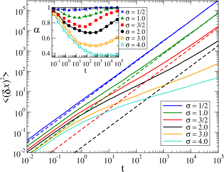
Figure 1: (Color online) Ensemble-averaged diffusion for different values of disorder strength $\sigma$ in units of $k_{B}T$ for exponentially decaying correlations. In doing numerics, we fixed $\sigma=\sigma_{0}$ and varied temperature. Distance is measured in units of correlation length $\lambda$ and time in units of $\tau_{0}=\lambda^{2}\eta/\sigma_{0}$. For $\sigma_{0}=2\,k_{B}T_{\rm room}=0.05$ eV, $D_{0}=k_{B}T_{\rm room}/\eta=3\;\mu m^{2}/s$, and $\lambda=5.25$ nm (15 bp), $\tau_{0}\approx 4.6\;\mu s$. Initially, diffusion is normal, $\langle\delta x^{2}(t)\rangle=2D_{0}t$. The dashed lines present asymptotically normal behavior $\langle\delta x^{2}(t)\rangle=2D_{\rm ren}t$, for $\sigma/(k_{B}T)=1/2,1,3/2,2$. Transient subdiffusion is much faster than this limit! Averaging over $10^{4}$ particles is done in 10 different realizations of random potential replicated with period $L=10^{4}$ ($10^{3}$ particles per a potential realization). Particles are initially uniformly distributed over the length $L$.

We focus on short-ranged correlations, which seemingly justified the use of the approximation of uncorrelated disorder in the bulk of previous research work DeGennes ; Zwanzig ; HTB90 . Even here, with growing $\sigma$ diffusion becomes transiently anomalous, $\langle\delta x^{2}(t)\rangle\propto t^{\alpha(t)}$, with a time-dependent $0<\alpha(t)\leq 1$. It starts from $\alpha=1$ at $t=0$ and tends to $\alpha=1$ asymptotically, see inset in Fig. 1. The time duration and spatial extension of subdiffusion depend very strongly on $\sigma$. For example, for $\sigma=4$ in Fig. 1, there is no any signature of growing $\alpha(t)$ on the whole time scale of simulation. Indeed, $\alpha\approx 0.4$ for $10^{3}<t<10^{5}$. The emergence of this subdiffusion is due to a transient breaking of ergodicity. Importantly, it is also non-Gaussian in subdiffusive regime, see Fig. S2 in Supplement . There exists an ergodicity length $L_{\rm erg}(\sigma)$, such that self-averaging occurs only for $L\gg L_{\rm erg}(\sigma)$. However, no self-averaging occurs on the mesoscale defined by the requirement that the above EBP equals one, which leads to the condition

$$\int_{0}^{1}\left(1-y\right)e^{\beta^{2}\sigma^{2}g(Ly)}dy=1\;.$$ (7)

Solution of this equation for unknown $L$ gives $L_{\rm erg}$. Another estimation yields $L_{\rm erg}(\sigma)\sim\lambda e^{\sigma^{2}/(k_{B}T)^{2}}$ SlutskyPRE , which indeed displays a major trend with $\sigma$. For example, for $\sigma=2$, Eq. (7) yields $L_{\rm erg}(2)\approx 35\lambda$ (while $e^{4}\approx 54.6$). This indeed is consistent with the trend one observes in Fig. 1 for $\sigma=2$, where $\langle\delta x^{2}(t_{\rm max})\rangle\sim 3000\lambda^{2}$. In this respect, a recent experiment shows that 1d diffusion along DNA is suppressed by the factor of hundred with respect to one in the bulk Elf . This suggests $\sigma\sim 2\,k_{B}T_{\rm room}\sim 0.05$ eV with experimental values $D_{0}=3\;\mu m^{2}/s$ and $D_{\rm ren}=0.046\;\mu m^{2}/s$ Elf . Applying this result to diffusion of a protein on DNA with $\lambda=15$ bp suggests that protein diffusion should be still anomalous on a typical gene length about 1000 bp. Remarkably, another experiment reveals even a larger suppression factor of about $10^{4}$ Wang , which would correspond to $\sigma\sim 3\;k_{B}T_{\rm room}$. Then, from Eq. (7) $L_{\rm erg}(3)\approx 2070\;\lambda$ (while $e^{9}\approx 8103$), a drastic increase! This would mean that a typical subdiffusion length would cover about 30-120 genes in bacterial genome, which can have important consequences for gene regulation. In a more general context, already for $\sigma=4\,k_{B}T$, $L_{\rm erg}(4)\sim 1.2\cdot 10^{6}\lambda$, i.e. for $\lambda\sim 10$Å, $L_{\rm erg}(4)\sim 1.2$ mm, i.e. subdiffusion reaches clearly a macroscale. Other models of decaying correlations cannot change much this conclusion. Then, the classical result in Eq. (5) can mislead, even being formally valid.

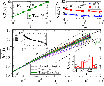
Figure 2: (Color online) (a) Single-trajectory averages are scattered between the free and disorder-renormalized diffusion limits (depicted with dashed-dotted lines). Time window ${\rm T_{w}}=2\cdot 10^{4}$ for averaging is chosen 100x larger than the maximal time $t$. Each trajectory is characterized by individual subdiffusion index $\alpha$ distributed as shown in the lower inset. Arrow indicates the value of $\alpha=0.67$ which corresponds to the ensemble average depicted with dashed line. The ensemble average of time-averages with $\alpha=0.78$ is depicted as full green line. It is also depicted in part (b) as function of time $t$ for ${\rm T_{w}}=10^{4}$, and also in part (c) as function of ${\rm T_{w}}$ for two fixed values of $t$. The latter one decays as $\Big{\langle}\overline{\delta x^{2}(t)}\Big{\rangle}\sim{\rm T_{w}}^{-0.07}$. Moreover, the corresponding ergodicity breaking parameter in the upper inset of part (a) gradually decays as a function of ${\rm T_{w}}$. This indicates that no ergodicity breaking takes place asymptotically, ${\rm T_{w}}\to\infty$.

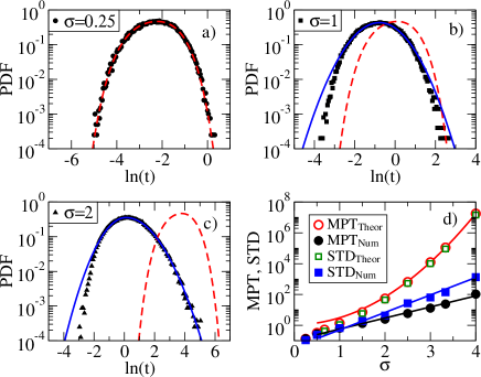
Figure 3: (Color online)(a,b,c) Probability density of waiting times derived from numerics (symbols), its fit with a log-normal distribution (full lines), and the result expected from normal diffusion with $D_{\rm ren}$ (dashed lines) for three different values of $\sigma/k_{B}T$, (d) Mean first passage time (MPT) and its standard deviation (STD) derived from numerics (symbols) and their exponential fits (full lines), as well as MPT and STD expected from normal diffusion characterized by $D_{\rm ren}$, which obey a $const\times\exp[-\sigma^{2}/(k_{B}T)^{2}]$ dependence.

Given nonergodic origin of such subdiffusion it becomes important to study single-trajectory averages, $\overline{\delta x^{2}(t)}^{\rm T_{w}}:=[1/({\rm T_{w}}-t)]\int_{0}^{{\rm T_{w}}-t}[\delta x(t|t^{\prime})]^{2}dt^{\prime}$, of the mean-squared displacement, $\delta x(t|t^{\prime})=x(t+t^{\prime})-x(t^{\prime})$, over a time window, ${\rm T_{w}}$, assuming $t\ll{\rm T_{w}}$ Wang ; Golding . The results for $\sigma=2$ display a typical scatter in Fig. 2. It can be characterized by a broadly distributed subdiffusion exponent $\alpha$. Similar features are indeed seen in many experiments Golding . The corresponding ensemble average $\Big{\langle}\overline{\delta x^{2}(t)}^{\rm T_{w}}\Big{\rangle}$ is different from the standard ensemble average $\langle\delta x^{2}(t)\rangle$, having even a different anomalous exponent, see Fig. 2, a, b. Recent experimental findings Wang indirectly corroborate our results. Indeed, in Wang a huge scatter of the diffusional constants for LacI protein on a bacterial DNA has been reported, which the authors attributed to a wildly (over 3 orders of magnitude) distributed normal diffusion coefficient. When we increase $\sigma$ to $\sigma=3\;k_{B}T$, the scatter indeed further increases, see in Fig. S3 of Supplement .

Strikingly enough, all the single-trajectory averages reveal subdiffusion which proceeds much faster than expected from Eq. (5), see in Fig. 2, a. It must be emphasized that even though our results somewhat remind ones obtained for CTRW subdiffusion with divergent mean residence times, or with exponential energy disorder CTRWage , in fact, they are very different. First, also single trajectory averages yield subdiffusion (without any boundary effects). Second, the drift of these averages with growing time window ${\rm T_{w}}$ is much less pronounced. see in Fig. 2, c. Moreover, the related EBP shows a clear tendency to zero with increasing ${\rm T_{w}}$, cf. inset in Fig. 2, a.

Especially important is that the corresponding residence time distribution to stay in any finite-size spatial domain is neither featured by diverging mean residence time, nor by diverging variance. In this respect, our results also essentially differ from the results in Khoury . They are somewhat closer in this particular aspect to viscoelastic subdiffusion. However, the latter one is mostly ergodic by its origin Goychuk09 , and therefore is also different. We investigate the distribution of escape times out of spatial domain $[-\lambda,\lambda]$ for the particles initially localized in the middle of it. For disorder-renormalized normal diffusion the residence time distribution can be derived as $\psi(t)=\pi\sum_{n=0}^{\infty}(-1)^{n}(2n+1)e^{-\pi^{2}(2n+1)^{2}t/4}$, with time in units of $\lambda^{2}/D_{\rm ren}$. It is dominated by a single-exponential $\psi(t)\propto\pi\exp(-\pi^{2}t/4)$ at large times. For small disorder, this result is nicely confirmed numerically in Fig. 3, a, which provides also one of the successful tests of the accuracy of our numerics. However, already for $\sigma=k_{B}T$ essentially deviations are observed in Fig. 3, b. The mean time not only exists, but it is much smaller that one expects from normal diffusion, even though the distribution becomes broader than exponential. For a sufficiently large disorder, its essential part is nicely described by the log-normal distribution, $\psi(t)=1/(\sqrt{2\pi}\sigma_{\tau}t)\exp[-\ln^{2}(t/\tau_{0})/(2\sigma_{\tau}^{2})]$, with two parameters $\tau_{0}$ and $\sigma_{\tau}$, which are related to the finite mean and variance of this distribution depicted in Fig. 3, d. Such a distribution can be confused for a power law distribution, $\psi(t)\propto 1/t$, at short times. However, it is profoundly different. The numerical mean and variance are much smaller than those expected from disorder-renormalized normal diffusion. Moreover, they exhibit a linear dependence on $\sigma/(k_{B}T)$ in the exponential, i.e. $\propto\exp[\sigma/(k_{B}T)]$, rather than quadratic, i.e. $\propto\exp[\sigma^{2}/(k_{B}T)^{2}]$. Fig. 3, d illustrates this very important finding. Subdiffusional search due to spatial correlations is thus expected to proceed much faster that one naively expects from the well-known renormalization by disorder!

To conclude, we summarize the important findings of this work. First, the famous result in Eq. (5) remains valid asymptotically for any model of decaying correlations. Diffusion is suppressed by the factor responsible for well-known non-Arrhenius temperature dependence Hecksher . However, a similar factor characterizes also the spatial range of transient subdiffusion in units of the disorder correlation length $\lambda$. Second, subdiffusion readily reaches a macroscale even for a moderately strong disorder of $\sigma\sim 4-5\,k_{B}T$. Third, already for $\sigma\sim 2\,k_{B}T_{\rm room}\sim 0.05$ eV diffusion of regulatory proteins on DNAs becomes essentially anomalous on a typical length of genes, with a large scatter in single trajectory averages. Fourth, and the most surprising, such subdiffusion proceeds much faster than one expects when applies Eq. (5) to transport processes on mesoscale. We believe that these important findings provide a new vista on the role of correlations in Gaussian disorder and subdiffusion, and will inspire related experimental work.

Acknowledgment. Support of this research by the Deutsche Forschungsgemeinschaft (German Research Foundation), Grant GO 2052/1-2 is gratefully acknowledged.

References

- (1) J.-P. Bouchaud and A. Georges, Phys. Rep. 195, 127 (1990).
- (2) P. Hänggi, P. Talkner, and M. Borkovec, Rev. Mod. Phys. 62, 251 (1990).
- (3) B. D. Hughes, Random walks and Random Environments, Vols. 1,2 (Clarendon Press, Oxford, 1995).
- (4) R. Metzler and J. Klafter, Phys. Rep. 339, 1 (2000).
- (5) P. G. de Gennes, J. Stat. Phys. 12, 463 (1975).
- (6) R. Zwanzig, Proc. Natl. Acad. Sci. (USA) 85, 2029 (1988).
- (7) H. Bässler, Phys. Rev. Lett. 58, 767(1987).
- (8) H. Bässler, Phys. Stat. Sol. B 175, 15 (1993).
- (9) Th. A. Vilgis, J. Phys. C 21, L299 (1988).
- (10) T. Hecksher, A. I. Nielsen, N. B. Olsen, and J. C. Dyre, Nature Phys. 4, 737 (2008).
- (11) D. H. Dunlap, P. E. Parris, and V. M. Kenkre, Phys. Rev. Lett. 77, 542 (1996).
- (12) E. Schrödinger, What Is Life? The Physical Aspect of the Living Cell (Cambridge University Press, New York, 1944).
- (13) M. Lässig, BMC Bioinformatics 8(Suppl 6), S7 (2007).
- (14) M. Slutsky, M. Kardar, and L. A. Mirny, Phys. Rev. E. 69, 061903 (2004); ibid. 70, 049901(E) (2004).
- (15) A. J. Stewart, S. Hannenhalli, and J. B. Plotkin, Genetics 192, 973 (2012).
- (16) A. G. Cherstvy, A. B. Kolomeisky, and A. A. Kornyshev, J. Phys. Chem. B 112, 4721 (2008).
- (17) P. E. Parris, M. Kus, D. H. Dunlap, and V. M. Kenkre, Phys. Rev. E 56, 5295 (1997).
- (18) A. H. Romero and J. M. Sancho, Phys. Rev. E 58, 2833 (1998).
- (19) M. Khoury, A. M. Lacasta, J. M. Sancho, and K. Lindenberg, Phys. Rev. Lett. 106, 090602 (2011); K. Lindenberg, J. M. Sancho, M. Khoury, and A. M. Lacasta, Fluc. Noise Lett. 11, 1240004 (2012).
- (20) M. S. Simon, J. M. Sancho, and K. Lindenberg, Phys. Rev. E 88, 062105 (2013).
- (21) I. Goychuk, Fluct. Noise Lett. 11, 1240009 (2012); I. Goychuk, Phys. Rev. E 86, 021113 (2012).
- (22) See Supplemental Material online:
- (23) A. Papoulis, Probability, Random Variables, and Stochastic Processes, 3d ed. (McGraw-Hill Book Company, New York, 1991), Ch. 13.
- (24) W. H. Deng and E. Barkai, Phys. Rev. E 79, 011112 (2009).
- (25) J. Elf, G.-W. Li, and X. S. Xie, Science 316, 1191 (2007).
- (26) Y. M. Wang, R. H. Austin, and E. C. Cox, Phys. Rev. Lett. 97, 048302 (2006).
- (27) I. Golding and E. C. Cox, Phys. Rev. Lett. 96, 098102 (2006); J.-H. Jeon, et al., Phys. Rev. Lett. 106, 048103 (2011); S. M. A. Tabei, et al., Proc. Natl. Acad. Sci. USA 110 4911 (2013).
- (28) A. Lubelski, I. M. Sokolov, and J. Klafter, Phys. Rev. Lett. 100, 250602 (2008); Y. He, S. Burov, R. Metzler, and E. Barkai, Phys. Rev. Lett. 101, 058101 (2008); T. Miyaguchi and T. Akimoto, Phys. Rev. E 83, 031926 (2011); E. Barkai, Y. Garini, and R. Metzler, Phys. Today 65(8), 29 (2012).
-
(29)
I. Goychuk, Phys. Rev. E 80, 046125 (2009); I. Goychuk,
Adv. Chem. Phys. 150, 187 (2012).
Supplemental material
Random force and its regularization. Random force , which corresponds to the Gaussian potential modeled by the Ornstein-Uhlenbeck process, has autocorrelation function . It is singular at origin, and negatively correlated otherwise. The singularity makes wildly fluctuating, see Fig. 1S for a realization of this process obtained with a spectral method detailed in SimonFNL . Random realizations were obtained using fast Fourier transforms departing from the autocorrelation function (ACF), , as described in Ref. SimonFNL . The quality of potential realizations has been checked by numerical evaluation of ACF from the potential realizations and comparison it with the original, see inset in Fig. 1S. However, the singularity becomes smoothened due to the use of a space discretization step in simulations. Then, the maximal root mean square (rms) force fluctuation, , becomes finite, , which enables numerical simulations of this model by choosing sufficiently small integration time step , so that . This yields the criterion used to choose a proper time step in numerics done using stochastic Heun method on graphical processor units. Thereby, this singular model of spatial force correlations is effectively regularized as .Derivation of Eq. (3) of the main text. In order to find the transport coefficients in random potentials we consider the corresponding Fokker-Planck dynamics. The Fokker-Planck equation for the probability density is well known for any realization of random potential as a probability continuity equation![[Uncaptioned image]](/html/1406.4707/assets/x4.png)
FIG. 1S. One realization of random Gaussian potential with exponentially decaying correlations for (energy scale in simulations) and (length scale in simulations). Space discretization step , with linear interpolation between lattice points for the force (piecewise linear force, or piecewise parabolic potential). The inset shows excellent agreement between the model theoretical ACF and the numerical results.
with the probability flux . The flux reads in the transport form(8)
where is free diffusion coefficient, and is inverse temperature. We consider a periodic potential with spatial period which is quite natural for the protein diffusion on circular DNA molecules in bacteria (where also the generalized coordinate along DNA is cyclic). Under constant forcing , the stationary probability current will be eventually established. To find it, the spatially unbounded stationary dynamics can be asymptotically mapped onto the dynamics on a circle with period . This latter one can be easily solved by twice integrating Eq. (9) under the constant flux condition with periodic boundary conditions and , and normalization condition . This leads to the celebrated result by Stratonovich et al. Stratonovich for the mean particle velocity ,(9)
The nonlinear diffusion coefficient for vanishing bias readily follows from this result by the fluctuation-dissipation theorem, yielding Eq. (3) of the main text, upon using the imposed periodicity .(10) Non-Gaussian probability disribution in anomalous regime. Probability distribution is non-Gaussian in the regime of subdiffusion as displayed in Fig. 2S. It is well described by a generalized exponential distribution , with a time-dependent power exponent . Deviations of from the Gaussian value correlate with the occurrence of anomalous diffusion in Fig. 1 of the main text. Interestingly, the value of only weakly correlates with values of and anomalous exponent in the anomalous regime, compare the cases and in the inset. Ever increasing scatter of single-trajectory averages with increasing disorder. Single trajectory averages show ever larger scatter with increasing , see the case of in Fig. 3S. Notice that most trajectories are several orders of magnitude (!) faster than the classical result of disorder-renormalized normal diffusion coefficient predicts.![[Uncaptioned image]](/html/1406.4707/assets/x5.png)
FIG. 2S. Spatial distribution of particles at different times is described by a generalized exponential distribution, , with a time-dependent power exponent . Several snapshots of distribution are done for at various times, with varying in time as depicted in the inset, for several different values of . Notice that for the transition to normal Gaussian diffusion is accomplished on the time scale of simulations, while for , from till . Interestingly, does not seem to reflect the time dependence of . For example, for in Fig. 1 of the main text, in the time interval from till , while diminishes from about to about .

References

- (1) M. S. Simon, J. M. Sancho, and A. M. Lacasta, Fluct. Noise Lett. 11, 1250026 (2012).
- (2) R. L. Stratonovich, Topics in the Theory of Random Noise (Gordon and Breach, New York, 1963).