Bayesian estimation of discretely observed multi-dimensional diffusion processes using guided proposals

Abstract

Estimation of parameters of a diffusion based on discrete time observations poses a difficult problem due to the lack of a closed form expression for the likelihood. From a Bayesian computational perspective it can be casted as a missing data problem where the diffusion bridges in between discrete-time observations are missing. The computational problem can then be dealt with using a Markov-chain Monte-Carlo method known as data-augmentation. If unknown parameters appear in the diffusion coefficient, direct implementation of data-augmentation results in a Markov chain that is reducible. Furthermore, data-augmentation requires efficient sampling of diffusion bridges, which can be difficult, especially in the multidimensional case.

We present a general framework to deal with with these problems that does not rely on discretisation. The construction generalises previous approaches and sheds light on the assumptions necessary to make these approaches work. We define a random-walk type Metropolis-Hastings sampler for updating diffusion bridges. Our methods are illustrated using guided proposals for sampling diffusion bridges. These are Markov processes obtained by adding a guiding term to the drift of the diffusion. We give general guidelines on the construction of these proposals and introduce a time change and scaling of the guided proposal that reduces discretisation error. Numerical examples demonstrate the performance of our methods.

Keywords: Multidimensional diffusion bridge; data augmentation; discretisation of path integral; linear process; innovation process; non-centred parametrisation; FitzHugh-Nagumo model.

1 Introduction

In this article we discuss a novel approach for estimating an unknown parameter $\theta\in\Theta$ of the drift and the diffusion coefficient of a diffusion process

$${\,\mathrm{d}}X_{t}=b_{\theta}(t,X_{t}){\,\mathrm{d}}t+\sigma_{\theta}(t,X_{t}){\,\mathrm{d}}W_{t},\qquad X_{0}=u$$ (1.1)

which is observed discretely in time. Here $b_{\theta}\colon\mathbb{R}\times\mathbb{R}^{d}$ denotes the drift function, $a_{\theta}=\sigma_{\theta}\sigma_{\theta}^{\prime}$ is the diffusion function, where $\sigma_{\theta}\colon\mathbb{R}\times\mathbb{R}^{d}\to\mathbb{R}^{d\times d^{\prime}}$, and $W$ is a $d^{\prime}$-dimensional Wiener process. The observation times will be denoted by $t_{0}=0<t_{1}<\cdots<t_{n}=T$ and the corresponding observations by $x_{i}=X_{t_{i}}$.

Estimation of $\theta$ in this setting has attracted much attention during the past decade. Here we restrict attention to estimation within the Bayesian paradigm. From a theoretical perspective, results on posterior consistency have been proved in Van der Meulen and Van Zanten (2013) and Gugushvili and Spreij (2012). The associated computational problem is the object of study here. Two review articles that include many references on this topic are Van Zanten (2013) and Sørensen (2004).

The main difficulty in estimation for discretely observed diffusion processes is the lack of a closed form expression for transition densities, making the likelihood intractable. If the diffusion path is observed continuously, then estimation becomes easier as for a fully observed diffusion path the likelihood is available in closed form (and parameters appearing in the diffusion coefficient can be determined from the quadratic variation of the process). This naturally suggests to study the computational problem within a missing data framework, treating the unobserved path segments between two succeeding observation times as missing data. This setup dates back to at least Pedersen (1995), who used it to obtain simulated maximum likelihood estimates for $\theta$. Within the Bayesian computational problem, the resulting Markov-Chain-Monte-Carlo algorithm is known as data-augmentation and was introduced in this context by Eraker (2001), Elerian et al. (2001) and Roberts and Stramer (2001). This algorithm is a special form of the Gibbs sampler which iterates the following steps:

1. draw missing segments, conditional on $\theta$ and the observed discrete time data;

2. draw from the distribution of $\theta$, conditional on the “full data”.

Here, by “full data” we mean the path formed by the drawn segments joined at the observation times. The algorithm can be initialised by either interpolating the discrete time data or choosing an initial value for $\theta$. We now discuss tho major challenges for the outlined algorithm together with various solutions that have been proposed in the literature.

Challenge 1: generating “good” proposals for the missing segments. The problem of simulating diffusion bridges has received a lot of attention over the past 15 years. Vastly different techniques have been proposed, including (i) single site Gibbs updating of the missing segments locally on a discrete grid (Eraker (2001)), (ii) independent Metropolis-Hastings steps using as a proposal a Laplace approximation to the conditional distribution obtained by Euler approximation (Elerian et al. (2001)), (iii) forward simulated processes derived from representations of the Brownian bridge in discrete time (Durham and Gallant (2002)), (iv) coupling arguments (Bladt and Sørensen (2014) and Bladt and Sørensen (2015)), (v) a constrained sequential Monte Carlo algorithm with a resampling scheme guided by backward pilots (Lin et al. (2010)), and (vi) exact simulation (Beskos et al. (2006)).

Delyon and Hu (2006) extended the work of Durham and Gallant (2002) to a continuous time setup and derived an innovative proposal process taking the drift of the target diffusion into account. In case the diffusion coefficient is constant this proposal was proposed earlier in Clark (1990). The basic idea consists of superimposing an additional term to the drift of the unconditioned diffusion to guide the process towards the endpoint. Such proposals are termed guided proposals and have the advantage that only forward simulation of an SDE is required. More precisely, the drift of the proposal that hits $v\in\mathbb{R}^{d}$ at time $T$ equals $b^{\circ}(t,x)=\lambda b(t,x)+(v-x)/(T-t)$, where either $\lambda=0$ or $\lambda=1$ is chosen. If $\lambda=0$, the guiding term $(v-x)/(T-t)$ matches with the drift of the SDE for a Brownian bridge, which indeed has drift $0$. However, this proposal has the drawback that it is independent of the drift $b$ of the diffusion. If $\lambda=1$, the guiding term depends on $b$ and consequently there is a potential mismatch between the drift and guiding term. In both cases (i.e. $\lambda=0$ and $\lambda=1$) there can be a substantial mismatch between the proposals and true bridges, rendering low acceptance rates in an MH-sampler.

In Schauer et al. (2016) a general class of proposal processes for simulating diffusion bridges was introduced. The proposals in Schauer et al. (2016) do take the drift of the target diffusion into account, but in a way different from Delyon and Hu (2006). As a result, these proposals can substantially reduce the mismatch of drift and guiding term, because they allow for more flexibility in choosing an appropriate guiding term to pull the process towards the endpoint in the right manner. An example of the advantage of this approach is given in the introduction of Schauer et al. (2016). General guidelines to exploit the added flexibility are addressed in this paper.

For implementation purposes, any proposal has to be evaluated on a finite number of grid points. As the pulling term added to the drift for guided proposals has a singularity near the endpoint, special care is needed in choosing a discretisation method. More importantly, integrals that appear in the acceptance probability of bridges potentially suffer from this problem as well. In this paper we introduce a time change and scaling of the proposal process that deals with these problems.

Challenge 2: handling unknown parameters appearing in the diffusion coefficient. As pointed out by Roberts and Stramer (2001), the data augmentation algorithm degenerates if $\theta$ appears in the diffusion coefficient as the quadratic variation of the full data $\int_{0}^{T}a_{\theta}(t,X_{t}){\,\mathrm{d}}t$ forces the conditional distribution for the next iterate for $\theta$ to be degenerate at the current value. Hence, iterates of $\theta$ remain stuck at their initial value. The problem was solved in a discretised setting by both Chib et al. (2004) and Golightly and Wilkinson (2010). Rather than updating $\theta$ conditional on the discretised diffusion bridge, they proposed updating $\theta$ conditional on the increments of the Brownian motion driving the discretised diffusion bridge. This decouples the tight dependence between $\theta$ and the diffusion bridge. However, as Stramer and Bognar (2011) point out “While the promising GW approach can be applied to a large class of diffusions, it is not yet rigorously justified in the literature.” Put differently, whereas the GW (=Golightly-Wilkinson) approach works in the discretised setup, it gives no guarantee that it also works in the limit where the discretisation level tends to zero.

In the continuous-time framework a solution to the aforementioned problem was given in Roberts and Stramer (2001) for one-dimensional diffusions. It was extended to reducible multivariate diffusions (diffusions that can be transformed to have unit diffusion coefficient) in Beskos et al. (2006) and Sermaidis et al. (2013). The basic idea is that the laws of the bridge proposals can be understood as parametrised push forwards of the law of an underlying random process common to all models with different parameters $\theta$. This is naturally the case for proposals defined as solutions of stochastic differential equations and the driving Brownian motion can be taken as such underlying random process. If $X^{\star}$ denotes a missing segment given that the parameter equals $\theta$, the main idea consists of finding a map $g$ and a process $Z$ such that $X^{\star}=g(\theta,Z)$. In a more general set-up, decouplings of similar forms are discussed under the keyword non-centred parameterisation (Papaspiliopoulos et al. (2003)). The process $Z$ will be called the “innovation process” (analogous to terminology used in Chib et al. (2004) and Golightly and Wilkinson (2010)). Whereas in case $\sigma_{\theta}=\theta$ the construction is rather easy, in general proving existence of the map $g$ and process $Z$ is subtle and this forms an important topic of this paper. We postpone a detailed discussion to Sections 2 and 3.

A first attempt of finding a non-centred parameterisation in continuous time in a general setting was undertaken in Fuchs (2013) (in particular section 7.4). Fuchs (2013) works in the setting of Delyon and Hu (2006), so it is assumed that the diffusion coefficient $\sigma$ is invertible and the diffusion is time-homogeneous. While the results in Fuchs (2013) are formulated in continuous time, the derivation involves heuristic arguments via the Lebesgue densities of the finite dimensional distributions. A recent work is Papaspiliopoulos et al. (2013). In their approach the missing data is initially considered in continuous time using Delyon and Hu (2006) bridge proposals, but the degeneracy problem is tackled only after discretisation.

What is the essential structure behind those different approaches and how can the underlying transformations be handled in continuous time without resorting to discretisation? Are these techniques tied to certain proposals, for example the proposal processes in Delyon and Hu (2006), or are they valid for other proposal processes as well? And can conditions such as invertibility of $\sigma$ be relaxed and is it essential that the diffusion is time-homogeneous? Part of this paper consists of answering these questions in a rigorous way. As a result of this, in our setting it is evident how to replace the independence sampler for $Z$ (which updates the diffusion bridges) by a random-walk type update on the process $Z$ in a straightforward way.

1.1 Contribution

In this article we present a general framework for Bayesian estimation of discretely observed diffusion processes that satisfactory deals with both aforementioned challenges. Our approach reveals the conditions necessary for obtaining an irreducible Markov chain that samples from the posterior (after burnin). We show that the algorithm does not suffer from the degeneracy problem in case unknown parameters appear in the diffusion coefficient, not even in the continuous time setup. The procedure can be seen as extension and unification of previous approaches within a continuous time framework. For example the results of the rather complicated heuristics in Section 7.4 of Fuchs (2013) appear as a special case of our work. Specific features of our approach include:

• We use in each data augmentation step “adapted” bridge proposals which take both the drift and the value of $\theta$ at that particular iteration into account. Hence, at each iteration, the pulling term depends on $\theta$, a feature which is unavailable using proposals as in Delyon and Hu (2006). Especially in the multivariate case, the additional freedom in devising good proposals is crucial for obtaining a feasible MCMC procedure. The possibility to exploit special features of the drift function to achieve high acceptance rates makes this approach interesting for practitioners. This is illustrated with a practical example in Section 7.2.

• We provide specialised algorithms in case the drift is of the form $b_{\theta}(\cdot)=\sum_{i=1}^{N}\theta_{i}\varphi_{i}(\cdot)$ for known functions $\varphi_{1},\ldots,\varphi_{N}$ (Cf. algorithms 2 and 3).

• The innovation process is defined using the proposal process. As a result, in our algorithm (Cf. algorithm 1), the innovations actually never need to be computed. This implies that our method can also cope with the case where $\sigma$ is not a square matrix (which is not the case for example in Fuchs (2013)).

• We illustrate our work using linear guided proposals as introduced in Schauer et al. (2016) and the proposals introduced in Delyon and Hu (2006). In section 4.4 we give general guidelines on the construction of these proposals. In section 7.2 we show that not taking into account the drift of the diffusion can lead to extremely small acceptance probabilities for bridges.

• Though we derive all our results in a continuous time setup, for implementation purposes integrals in likelihood ratios and solutions to stochastic differential equations need to be approximated on a finite grid. As the drift of our proposal bridges has a singularity near its endpoint, we introduce a time change and scaling that allows for numerically accurate discretisation and evaluation of the likelihood.

The approach with linear guided proposals can be extended to the case of partially observed diffusions, where for example some components of the diffusion are unobserved. Though the problem becomes much harder, the underlying structure for constructing an algorithm is the same. For details we refer to van der Meulen and Schauer (2016).

1.2 Outline

In Section 2 we clarify the aforementioned difficulties in a toy example. Here, we set some general notation and introduce some key ideas used throughout. In section 3 we precisely state our algorithms and introduce the concept of a feasible proposal. In Section 4 we show that both the proposals from Delyon and Hu (2006) and Schauer et al. (2016) are feasible. In Section 4.4 we give guidelines on constructing a guiding term for the proposals from Schauer et al. (2016). Numerical discretisation issues and the computational complexity of the proposed algorithms are discussed in sections 5 and 6 respectively. Numerical examples are given in Section 7. The appendix contains a few postponed proofs.

2 A toy problem

In this section we consider a toy example to illustrate some key ideas to solve the aforementioned problems with a simple data-augmentation algorithm. The type of reparameterisation introduced shortly is not new, and has appeared for example in Roberts and Stramer (2001). The goal here is to introduce key ideas and point out some of its potential shortcomings in more complex problems. Furthermore, later on we will deal with more difficult cases and this toy example allows us to sequentially build up an appropriate framework for that. We consider the diffusion process

$${\,\mathrm{d}}X_{t}=b(X_{t}){\,\mathrm{d}}t+\theta{\,\mathrm{d}}W_{t},\quad X_{0}=u,\quad t\in[0,T],$$

where $b$ is a known drift function and $\theta\in\Theta$ an unknown scaling parameter. We assume $\theta$ is equipped with a prior distribution $\pi_{0}(\theta)$ and only one observation $X_{T}=v$ at time $T$ is available. We aim to draw from the posterior $\pi(\theta\mid X_{T})$. The diffusion process conditioned on $X_{T}=v$ is a diffusion process itself. Denote by $X^{\star}$ the conditioned diffusion path $(X_{t},\,t\in(0,T))$ (conditional on $X_{T}=v$). Suppose we wish to iterate a data-augmentation algorithm and the current iterate is given by $(X^{\star},\theta)$.

Updating $X^{\star}$: For almost all choices of $b$, there is no direct way of simulating $X^{\star}$. Instead, one can first generate a proposal bridge $X^{\circ}$ and accept with MH-acceptance probability. As an easy tractable example we choose to take

$${\,\mathrm{d}}X^{\circ}_{t}=\frac{v-X^{\circ}_{t}}{T-t}{\,\mathrm{d}}t++\theta{\,\mathrm{d}}W_{t},\quad X^{\circ}_{0}=u$$ (2.1)

where $W$ is a Brownian Motion on $[0,T]$.

Denote the laws of $X^{\circ}$ and $X^{\star}$ (viewed as Borel measures on $C([0,T],\mathbb{R}^{d})$) by $\mathbb{P}^{\circ}$ and $\mathbb{P}^{\star}$ respectively. We have

$$\frac{{\,\mathrm{d}}\mathbb{P}^{\star}_{\theta}}{{\,\mathrm{d}}\mathbb{P}^{\circ}_{\theta}}(X^{\circ})=\frac{\widetilde{p}_{\theta}(0,u;T,v)}{p_{\theta}(0,u;T,v)}\Psi_{\theta}(X^{\circ}),$$ (2.2)

with

$$\Psi_{\theta}(X^{\circ})=\exp\left(\theta^{-2}\int_{0}^{T}b(X^{\circ}_{s}){\,\mathrm{d}}X^{\circ}_{s}-\frac{1}{2}\theta^{-2}\int_{0}^{T}b(X^{\circ}_{s})^{2}{\,\mathrm{d}}s\right).$$

Here, $p$ denotes the transition densities of the process $X$ and $\widetilde{p}(0,u;T,v)=\varphi(v;u,\theta^{2}T)$ (the density of the $N(u,\theta^{2}T)$-distribution, evaluated at $v$). Absolute continuity is a consequence of Girsanov’s theorem applied to the unconditioned processes and the abstract Bayes’ formula. Now the MH-step consists of generating a proposal $X^{\circ}$ and accepting it with probability $1\wedge\left(\Psi_{\theta}(X^{\circ})/\Psi_{\theta}(X^{\star})\right)$ (the ratio of transition densities just acts as a proportionality constant here).

Updating $\theta$: As explained in the introduction, taking the missing segment as missing data yields the Metropolis-Hastings algorithm reducible. To deal with this problem, note that by equation (2.1), there exists a mapping $g$ such that $X^{\circ}=g(\theta,W)$. Define the process $Z$ by the relation

$$X^{\star}=g(\theta,Z).$$ (2.3)

Now that $Z$ is defined, rather then drawing from the distribution of $\theta$ conditional on $(X_{0}=u,X_{T}=v,X^{\star})$ we will sample from the the distribution of $\theta$ conditional on $(X_{0}=u,X_{T}=v,Z)$. This means that we augment the discrete time observations with $Z$ instead of $X^{\star}$. Denote the laws of $Z$ and $W$ by $\mathbb{Z}_{\theta}$ and $\mathbb{W}$ respectively. Suppose the current iterate is $(\theta,Z)$, where $Z$ can be extracted from $\theta$ and $X^{\star}$ by means of equation (2.3). The following diagram summarises the notation introduced:

Process $$Z\stackrel{{\scriptstyle g(\theta,\cdot)}}{{\longrightarrow}}X^{\star}$$

Measure

(2.4)

For updating $\theta$ we propose a value ${\theta^{\circ}}$ from some proposal distribution $q(\cdot\mid\theta)$ and accept the proposal with probability $\min(1,A)$, where

$$A=\frac{\pi_{0}({\theta^{\circ}})}{\pi_{0}(\theta)}\frac{p_{\theta^{\circ}}(0,u;T,v)}{p_{\theta}(0,u;T,v)}\frac{{\,\mathrm{d}}\mathbb{Z}_{\theta^{\circ}}}{{\,\mathrm{d}}\mathbb{Z}_{\theta}}(Z)\frac{q(\theta\mid{\theta^{\circ}})}{q({\theta^{\circ}}\mid\theta)}.$$ (2.5)

Here, we have implicitly assumed that $\mathbb{Z}_{\theta^{\circ}}$ and $\mathbb{Z}_{\theta}$ are equivalent, which is indeed the case as we have

$$\frac{{\,\mathrm{d}}\mathbb{Z}_{\theta^{\circ}}}{{\,\mathrm{d}}\mathbb{Z}_{\theta}}(Z)=\frac{{\,\mathrm{d}}\mathbb{Z}_{\theta^{\circ}}}{{\,\mathrm{d}}\mathbb{W}}(Z)\bigg{/}\frac{{\,\mathrm{d}}\mathbb{Z}_{\theta}}{{\,\mathrm{d}}\mathbb{W}}(Z)=\frac{{\,\mathrm{d}}\mathbb{P}^{\star}_{\theta^{\circ}}}{{\,\mathrm{d}}\mathbb{P}^{\circ}_{\theta^{\circ}}}(g({\theta^{\circ}},Z))\bigg{/}\frac{{\,\mathrm{d}}\mathbb{P}^{\star}_{\theta}}{{\,\mathrm{d}}\mathbb{P}^{\circ}_{\theta}}(g(\theta,Z))$$

and thus results from absolute continuity of $\mathbb{P}^{\star}_{\theta}$ and $\mathbb{P}^{\circ}_{\theta}$. By equation (2.2), we now get

$$\frac{{\,\mathrm{d}}\mathbb{Z}_{\theta^{\circ}}}{{\,\mathrm{d}}\mathbb{Z}_{\theta}}(Z)=\frac{p_{\theta}(0,u;T,v)}{p_{\theta^{\circ}}(0,u;T,v)}\frac{\widetilde{p}_{\theta^{\circ}}(0,u;T,v)}{\widetilde{p}_{\theta}(0,u;T,v)}\frac{\Psi_{\theta^{\circ}}(g({\theta^{\circ}},Z))}{\Psi_{\theta}(g(\theta,Z))}.$$

Substituting this expression into equation (2.5) yields

$$A=\frac{\pi_{0}({\theta^{\circ}})}{\pi_{0}(\theta)}\frac{\widetilde{p}_{\theta^{\circ}}(0,u;T,v)}{\widetilde{p}_{\theta}(0,u;T,v)}\frac{\Psi_{{\theta^{\circ}}}(g({\theta^{\circ}},Z))}{\Psi_{\theta}(g(\theta,Z))}\frac{q(\theta\mid{\theta^{\circ}})}{q({\theta^{\circ}}\mid\theta)}$$ (2.6)

and all terms containing the unknown transition density cancel. In Section 4 we will show that cancellation of $p$ from the acceptance probability holds much more generally.

The feasibility and efficiency of this algorithm is crucially determined by choice of the transition kernel $q$ and proposal process $X^{\circ}$. We focus on an appropriate choice of $X^{\circ}$, though in section 3.3 we give guidelines on appropriate choice of $q$ if the drift possesses a specific structure with respect to $\theta$.

3 Proposed MCMC algorithms

Our starting point is that under weak assumptions the target diffusion bridge $X^{\star}$ from $u$ at time $t=0$ to $v$ at time $t=T$ is characterised as the solution to the SDE

$${\,\mathrm{d}}X^{\star}_{t}=b_{\theta}^{\star}(t,X^{\star}_{t}){\,\mathrm{d}}t+\sigma_{\theta}(t,X^{\star}_{t}){\,\mathrm{d}}W_{t},\qquad X^{\star}_{0}=u,\qquad t\in[0,T),$$ (3.1)

where

$$b^{\star}_{\theta}(t,x)=b_{\theta}(t,x)+a_{\theta}(t,x)\nabla_{x}\log p_{\theta}(t,x;T,v)$$ (3.2)

and $a=\sigma\sigma^{\prime}$. Here the transition density of $X$ is denoted by $p_{\theta}$ and $p_{\theta}(t,x;T,v)$ is the density of the process starting in $x$ at time $t$, ending in $v$ at time $T$.

3.1 Innovation process

Direct forward simulation of $X^{\star}$ is hardly ever possible, as $p$ is intractable. Instead, we propose to simulate a process $X^{\circ}$ with induced law that is absolutely continuous with respect to that of $X^{\star}$. More precisely, we assume the proposal process $X^{\circ}$ satisfies the SDE

$${\,\mathrm{d}}X^{\circ}_{t}=b_{\theta}^{\circ}(t,X^{\circ}_{t}){\,\mathrm{d}}t+\sigma_{\theta}(t,X^{\circ}_{t}){\,\mathrm{d}}W_{t},\qquad X^{\circ}_{0}=u,\qquad t\in[0,T)$$ (3.3)

We now describe a general parametrisation to decouple the dependence between the latent paths of the diffusion between discrete time observations and the parameter $\theta$.

The following proposition is key to the definition of the map $g$. In its statement we refer to the canonical setup on which an exact SDE can be solved, details are in section V.10 of Rogers and Williams (2000).

Proposition 3.1.

Assume

• the SDEs for $X^{\circ}$ and $X^{\star}$ are pathwise exact (in the sense of definition V-9.4 of Rogers and Williams (2000));

• there exists a strong solution for the SDE for $X^{\circ}$ (in the sense of definition V.10.9 of Rogers and Williams (2000)) jointly measurable with respect to starting point, parameter and path $W$;

• $\mathbb{P}^{\circ}$ and $\mathbb{P}^{\star}$ are absolutely continuous.

Then there exists a map $g$ and a Wiener process $W$ such that $X^{\circ}=g(\theta,W)$ on the canonical setup. Furthermore, there exists a process $Z$ such that $X^{\star}=g(\theta,Z)$. The process $Z$ satisfies the SDE

$${\,\mathrm{d}}Z_{t}=\mu_{\theta}\big{(}Z_{t}\big{)}{\,\mathrm{d}}t+{\,\mathrm{d}}W_{t}$$ (3.4)

where the map $\mu_{\theta}$ satisfies

$$\sigma_{\theta}(t,x)\mu_{\theta}(t,x)=b_{\theta}^{\star}(t,x)-b_{\theta}^{\circ}(t,x).$$ (3.5)

Moreover,

$${\,\mathrm{d}}X^{\star}_{t}=b^{\circ}_{\theta}(t,X^{\star}_{t}){\,\mathrm{d}}t+\sigma_{\theta}(t,X^{\star}_{t}){\,\mathrm{d}}Z_{t},\qquad X^{\star}_{0}=u,\qquad t\in[0,T).$$ (3.6)

Proof.

Denote the law of $W$ by $\mathbb{W}$. Existence of $g$ such that $X^{\circ}=g(\theta,W)$ is implied by existence of a strong solution for the SDE for $X^{\circ}$. If $Y$ satisfies

$${\,\mathrm{d}}Y_{t}=b_{\theta}^{\circ}(t,Y_{t}){\,\mathrm{d}}t+\sigma_{\theta}(t,Y_{t}){\,\mathrm{d}}W_{t},\qquad Y_{0}=u,\qquad t\in[0,T)$$

then $Y=g(\theta,W)$. Define

$$L_{\theta}=\exp\left(\int_{0}^{T}\mu_{\theta}(t,Y_{t}){\,\mathrm{d}}W_{t}-\int_{0}^{T}\mu_{\theta}(t,Y_{t})^{2}{\,\mathrm{d}}t\right)$$

and assume for the moment that $E^{\mathbb{W}}L_{\theta}=1$. Define the measure $\mathbb{Z}_{\theta}$ by ${\,\mathrm{d}}\mathbb{Z}_{\theta}=L_{\theta}{\,\mathrm{d}}\mathbb{W}$. By Girsanov’s theorem, it follows that the process $Z$ defined by equation (3.4) is a Brownian Motion under the measure $\mathbb{Z}_{\theta}$. If we define $Y$ by $Y=g(\theta,Z)$ then

$${\,\mathrm{d}}Y_{t}=b_{\theta}^{\circ}(t,Y_{t}){\,\mathrm{d}}t+\sigma_{\theta}(t,Y_{t}){\,\mathrm{d}}Z_{t},\qquad Y_{0}=u,\qquad t\in[0,T)$$

under $\mathbb{Z}_{\theta}$. Plugging (3.4) into this equation shows that

$${\,\mathrm{d}}Y_{t}=b^{\star}_{\theta}(t,Y_{t}){\,\mathrm{d}}t+\sigma_{\theta}(t,Y_{t}){\,\mathrm{d}}W_{t},\qquad Y_{0}=u,\qquad t\in[0,T).$$

By pathwise uniqueness $Y=X^{\star}$ up to indistinguishability under $\mathbb{W}$ (because $W$ is a Wiener process). Hence, $X^{\star}=g(\theta,Z)$ and (3.6) follows. We have

$$\frac{{\,\mathrm{d}}\mathbb{Z}_{\theta}}{{\,\mathrm{d}}\mathbb{W}}(\cdot)=\frac{{\,\mathrm{d}}\mathbb{P}_{\theta}^{\star}}{{\,\mathrm{d}}\mathbb{P}_{\theta}^{\circ}}(g(\theta,\cdot))$$ (3.7)

and henceforth existence of $\mu_{\theta}$ such that $E^{\mathbb{W}}L_{\theta}=1$ follows from our assumption that $\mathbb{P}^{\star}_{\theta}$ and $\mathbb{P}^{\circ}_{\theta}$ are absolutely continuous. ∎

We refer to the process $Z$ as the innovation process corresponding to $X^{\star}$ (by analogy of the terminology of Golightly and Wilkinson (2010) and Chib et al. (2004)). Clearly, $X^{\star}$ is related to $Z$ just like $X^{\circ}$ is related to $W$. Note however that while the law of $W$ does not depend on $\theta$ under $\mathbb{W}$, the law of $Z$ does depend on $\theta$ under $\mathbb{W}$.

In the following we will denote the Radon-Nikodym derivative between $\mathbb{P}^{\circ}$ and $\mathbb{P}^{\star}$ by $\Phi$:

$$\Phi_{\theta}:=\frac{{\,\mathrm{d}}\mathbb{P}_{\theta}^{\star}}{{\,\mathrm{d}}\mathbb{P}_{\theta}^{\circ}}.$$

3.2 Algorithm

In this section we present an algorithm to sample from the posterior of $\theta$ given the discrete observations ${\mathcal{D}}=\{X_{0}=u,X_{t_{1}}=x_{1},\ldots,X_{t_{n}}=x_{n}\}$. Denote the prior density on $\theta$ by $\pi_{0}$ and let $q(\theta^{\circ}\mid\theta)$ be the density for proposing $\theta^{\circ}$ given the current value $\theta$. The idea is to define a Metropolis–Hastings sampler on $(\theta,Z)$ instead of $(\theta,X^{\star})$ where $Z$ is the innovation process from the previous section.

More precisely, we construct a Markov chain for $(\theta,(Z_{i})_{1\leq i\leq n})$, where each $Z_{i}$ is an innovation process corresponding to the bridge $X^{\star}_{i}$ connecting observation $x_{i-1}$ to $x_{i}$.

Algorithm 1.

1. Initialisation. Choose a starting value for $\theta$ and sample $i=1,\dots,n$ Wiener processes $W_{i}$ and set $Z_{i}=W_{i}$.

2. Update $Z\mid(\theta,{\mathcal{D}})$. Independently, for $1\leq i\leq n$ do

   1. Sample a Wiener process $Z^{\circ}_{i}$.

   2. Sample $U\sim{\mathcal{U}}(0,1)$. Compute

      $$A_{1}=\frac{\Phi_{\theta}(g(\theta,Z^{\circ}_{i}))}{\Phi_{\theta}(g(\theta,Z_{i}))}.$$

      Set

      $$Z_{i}:=\begin{cases}Z^{\circ}_{i}&\text{if}\quad U\leq A_{1}\\ Z_{i}&\text{if}\quad U>A_{1}\end{cases}.$$

3. Update $\theta\mid(Z,{\mathcal{D}})$.

   1. Sample ${\theta^{\circ}}\sim q(\cdot\mid\theta)$.

   2. Sample $U\sim{\mathcal{U}}(0,1)$. Compute

      $$A_{2}=\frac{q(\theta\mid{\theta^{\circ}})}{q({\theta^{\circ}}\mid\theta)}\frac{\pi_{0}({\theta^{\circ}})}{\pi_{0}(\theta)}\prod_{i=1}^{n}\frac{p_{{\theta^{\circ}}}(t_{i-1},x_{i-1};t_{i},x_{i})}{p_{\theta}(t_{i-1},x_{i-1};t_{i},x_{i})}\frac{\Phi_{\theta^{\circ}}(g({\theta^{\circ}},Z_{i}))}{\Phi_{\theta}(g(\theta,Z_{i}))}$$

      Set

      $$\theta:=\begin{cases}{\theta^{\circ}}&\text{if}\quad U\leq A_{2}\\ \theta&\text{if}\quad U>A_{2}\end{cases}.$$

4. Repeat steps (2) and (3).

Note that in none of these steps we need to compute innovations $Z$ from $X^{\star}$. This is a consequence of adapting the definition of the innovations to the bridge proposals being used.

In step (2) an independent Metropolis-Hastings step is used. Instead, one can also propose $Z^{\circ}$ based on the current value of $Z$ in the following way

$$Z^{\circ}_{t}=\sqrt{\rho}Z_{t}+\sqrt{1-\rho}W_{t},$$ (3.8)

where $\rho\in[0,1)$ and $W$ is a Wiener process under $\mathbb{W}$ that is independent of $Z$. In this case

$$A_{1}=\frac{\left(\!{\,\mathrm{d}}\mathbb{Z}_{\theta}\big{/}\!{\,\mathrm{d}}\mathbb{W}\right)(Z)}{\left(\!{\,\mathrm{d}}\mathbb{Z}_{\theta}\big{/}\!{\,\mathrm{d}}\mathbb{W}\right)(Z^{\circ})}\frac{{\,\mathrm{d}}Q_{\rho}}{{\,\mathrm{d}}Q^{T}_{\rho}}(Z^{\circ},Z),$$

where $Q_{\rho}(x,y)=Q_{\rho}^{T}(y,x)$. Here we use the general formulation of the Metropolis-Hastings algorithm as explained in Tierney (1998). The second term equals one by symmetry of $Q(\cdot,\cdot)$. This implies that the acceptance probability in step 2(b) remains the same.

Remark 3.2.

Different proposals can be obtained by varying $b^{\circ}$ in (3.3) and it is clear that the mapping $g$ varies accordingly. A good choice obviously affects the acceptance probability of step 2 in algorithm 1. However, it affects the acceptance probability of step 3 as well as this step is a joint update of $(\theta,X^{\star})$. This implies that a proposal $\theta^{\circ}$ in step 3 which is “good” (in the sense of being like a draw from the posterior of $\theta$), may nevertheless be rejected if the mapping $g$ is such that $g(\theta^{\circ},Z)$ does not resemble a bridge with drift and diffusion coefficient indexed by $\theta^{\circ}$. Ideally, one would take $g=g_{\rm opt}$, where $g_{\rm opt}$ is defined by the relation $X^{\star}=g_{\text{\rm opt}}(\theta,W)$, with $W$ denoting a Wiener process.

Theorem 3.3.

Suppose $q(\theta^{\circ}\mid\theta)$ is almost everywhere strictly positive on the support of the prior for $\theta$. Then the chain induced by algorithm 1 is irreducible.

Proof.

Step 2 constitutes a step of a MH-sampler with independent proposals. The expression for $A_{1}$ follows directly from equation (3.7). The expression for $A_{2}$ in step 3 follows in exactly the same way as equation (2.6) was established in the toy-example (Cf. section 2). The remaining observation needed is the following: As $\Phi_{\theta}$ is the Radon-Nikodym derivative between two equivalent distributions, it is almost surely strictly positive and finite. Since the transition densities are strictly positive as well, both $A_{1}$ and $A_{2}$ are strictly positive and the result follows. ∎

At first sight, it may seem that algorithm 1 is not of much practical value. First of all, the mapping $g$ is unknown. However, as any algorithm derived in continuous time ultimately has to be approximated by discretisation, we can choose a discretisation level and compute $Y=g(\theta,Z)$ on a fine grid by discretising the stochastic differential equation

$${\,\mathrm{d}}Y_{t}=b^{\circ}_{\theta}(t,Y_{t}){\,\mathrm{d}}t+\sigma_{\theta}(t,Y_{t}){\,\mathrm{d}}Z_{t}.$$

Second, it seems impossible to compute the acceptance probabilities in steps 2 and 3 because $\Phi_{\theta}$ depends on $p$ and $p$ explicitly pops up in the formula for $A_{2}$. However, it turns out that for many choices of $b^{\circ}$ the unknown transition density $p$ only appears as a multiplicative constant in $\Phi_{\theta}$ such that it cancels the $p$ in the expression for $A_{2}$. For future reference, we introduce the following definition.

Definition 3.4.

We call a proposal $X^{\circ}$ as defined in equation (3.3) feasible if $b^{\circ}_{\theta}$ is such that both $A_{1}$ and $A_{2}$ appearing in algorithm 1 do not depend on the transition density $p$.

In section 4 we will give examples of classes of feasible proposals.

3.3 Partially conjugate series prior for the drift

In this subsection we study specific cases of algorithm 1 when the drift is of the form

$$b_{\vartheta}(x)=\sum_{i=1}^{N}\vartheta_{i}\varphi_{i}(x)$$ (3.9)

where $\vartheta=(\vartheta_{1},\ldots,\vartheta_{N})$ is an unknown parameter and $\varphi_{1},\ldots,\varphi_{N}$ are known functions on $\mathbb{R}^{d}$. We assume the diffusion coefficient is parametrised by the parameter $\gamma$. We denote the vector of all unknown parameters by $\theta=(\vartheta,\gamma)$ and assume these are assigned independent priors. With slight abuse of notation we use $\pi_{0}(\vartheta)$ and $\pi_{0}(\gamma)$ to denote the priors on $\vartheta$ and $\gamma$ respectively (the argument in parentheses will clarify which prior is meant). In this case it is convenient to choose a conjugate Gaussian prior for the coefficients, $\vartheta_{i}\sim{\mathcal{N}}(0,\xi^{2}_{i})$, for positive scaling constants $\xi_{i}$. Priors for the drift obtained by specifying a prior distribution on $\vartheta$ were previously considered in Küchler and Sørensen (1997), Bladt and Sørensen (2014) and Van der Meulen et al. (2014). Upon completing the square, it follows that the distribution of $\vartheta$ conditional on $\gamma$ and the full path $Y$ of the diffusion is multivariate normal with mean vector $W_{\gamma}^{-1}\mu_{\gamma}$ and covariance matrix $W_{\gamma}^{-1}$. We define for $k,\ell\in\{1,\ldots,d\}$,

$$\mu_{\gamma}[k] =\int_{0}^{T}\varphi_{k}(Y_{t})^{\prime}a_{\gamma}^{-1}(Y_{t}){\,\mathrm{d}}Y_{t}$$

$$\Sigma_{\gamma}[k,\ell] =\int_{0}^{T}\varphi_{k}(Y_{t})^{\prime}a_{\gamma}^{-1}(Y_{t})\varphi_{\ell}(Y_{t}){\,\mathrm{d}}t$$

$$W_{\gamma} =\Sigma+{\operatorname{diag}}(\xi_{1}^{-2},\ldots,\xi_{N}^{-2}).$$

(For a vector $x\in\mathbb{R}^{n}$ we denote the $i$-th element by $x[i]$. To emphasise the dependence on $Y$ we sometimes also write $\mu_{\gamma}(Y)$, $W_{\gamma}(Y)$ etc). This leads to a natural adaptation of algorithm 1 from section 3.2.

Algorithm 2.

Steps 1, 2 and 4 as in algorithm 1. Assume that $\sigma$ is invertible. Step 3 is given by

1. Update $\gamma\mid(\vartheta,Z,{\mathcal{D}})$.

   1. Sample ${\gamma^{\circ}}\sim q(\cdot\mid\gamma)$.

   2. Sample $U\sim{\mathcal{U}}(0,1)$. Compute

      $$A_{3}=\frac{q(\gamma\mid{\gamma^{\circ}})}{q({\gamma^{\circ}}\mid\gamma)}\frac{\pi_{0}({\gamma^{\circ}})}{\pi_{0}(\gamma)}\prod_{i=1}^{n}\frac{p_{({\gamma^{\circ}},\vartheta)}(t_{i-1},x_{i-1};t_{i},x_{i})}{p_{(\gamma,\vartheta)}(t_{i-1},x_{i-1};t_{i},x_{i})}\frac{\Phi_{({\gamma^{\circ}},\vartheta)}(g(({\gamma^{\circ}},\vartheta),Z_{i})}{\Phi_{(\gamma,\vartheta)}(g((\gamma,\vartheta),Z_{i}))}$$

      Set

      $$\gamma:=\begin{cases}{\gamma^{\circ}}&\text{if}\quad U\leq A_{3}\\ \gamma&\text{if}\quad U>A_{3}\end{cases}.$$

2. Update $\vartheta\mid(\gamma,Z,{\mathcal{D}})$.

   1. Compute $\mu_{g}=\mu_{\gamma}(g((\vartheta,\gamma),Z))$ and $W_{\gamma}=W_{\gamma}(g((\vartheta,\gamma),Z))$.

   2. Sample ${\vartheta^{\circ}}\sim{\mathcal{N}}(W_{\gamma}^{-1}\mu_{\gamma},W_{\gamma}^{-1})$.

   3. Compute $Z^{\circ}$ such that $g(({\vartheta^{\circ}},\gamma),Z^{\circ})=g((\vartheta,\gamma),Z)$. Set $\vartheta=\vartheta^{\circ}$ and $Z=Z^{\circ}$.

Note that computation of $Z^{\circ}$ in step 3.2(c) requires invertibility of $\sigma$.

Proof.

Suppose $(\vartheta,\gamma,Z)\sim\pi$, where $\pi$ denotes the posterior distribution. Consider the map $f\colon(\vartheta,\gamma,Z)\mapsto(\vartheta,\gamma,X^{\star})$, where $X^{\star}=g((\vartheta,\gamma),Z)$. We show that step 3.2 preserves $\pi$. The distribution of $(\vartheta,\gamma,X^{\star})$ is the image measure of the posterior distribution $\pi$ of the tuple $(\vartheta,\gamma,Z)$ under $f$ and coincides with the posterior distribution of $(\vartheta,\gamma,X^{\star})$. Denote the image measure of $\pi$ under $f$ by by $\pi\circ f^{-1}$. In steps 3.2(a) and 3.2(b) we apply the mapping $f$, followed by a Gibbs step in which we draw $\vartheta^{\circ}$ conditional on $(\gamma,X^{\star})$. The latter preserves $\pi\circ f^{-1}$. Hence $(\vartheta^{\circ},\gamma,X^{\star})\sim\pi\circ f^{-1}$. In step 3.2(c) we we compute $(\vartheta^{\circ},\gamma,Z^{\circ})$ as pre-image of $(\vartheta^{\circ},\gamma,X^{\star})$ under $f$ (this is possible as we assume $\sigma$ to be invertible). Hence $(\vartheta^{\circ},\gamma,Z^{\circ})\sim\pi$. ∎

A variation of this algorithm is obtained in case the drift is of the form specified in equation (3.9) and the diffusion coefficient depends on both $\vartheta$ and $\gamma$. In this case we can update $\gamma$ just as in algorithm 2. Updating $\vartheta$ can be done using a random walk type proposal of the form

$$q(\vartheta^{\circ}\mid\vartheta)\sim N(\vartheta,\alpha V),$$

with $\alpha$ a positive tuning parameter. Motivated by the covariance matrix of the prior exploited in the case of partial conjugacy we propose to replace $V$ by $W^{-1}_{(\vartheta,\gamma)}$. By this choice, if two components $\vartheta_{i}$ and $\vartheta_{j}$ are strongly correlated, the proposed local random walk proposals have the same correlation structure, which can improve mixing of the chain.

Algorithm 3.

The same algorithm as Algorithm 2 without the invertibility assumptions and Step 3.2 replaced by

1. Update $\vartheta\mid(\gamma,Z,{\mathcal{D}})$.

   1. Set $X^{\star}=g(\vartheta,Z)$.

   2. Compute $W_{(\vartheta,\gamma)}$.

   3. Sample ${\vartheta^{\circ}}\sim{\mathcal{N}}(\vartheta,\alpha^{2}W_{(\vartheta,\gamma)}^{-1})$.

   4. Compute $W_{({\vartheta^{\circ}},\gamma)}$.

   5. Sample $U\sim{\mathcal{U}}(0,1)$. Compute

      $$A_{4} =\frac{|W_{{\vartheta^{\circ}}}|^{1/2}}{|W_{\vartheta}|^{1/2}}\exp\left(-\frac{1}{2\alpha^{2}}({\vartheta^{\circ}}-\vartheta)^{\prime}(W_{\vartheta^{\circ}}-W_{\vartheta})({\vartheta^{\circ}}-\vartheta)\right)$$

      $$\qquad\times\frac{\pi_{0}({\vartheta^{\circ}})}{\pi_{0}(\vartheta)}\prod_{i=1}^{n}\frac{p_{(\gamma,{\vartheta^{\circ}})}(t_{i-1},x_{i-1};t_{i},x_{i})}{p_{(\gamma,\vartheta)}(t_{i-1},x_{i-1};t_{i},x_{i})}\frac{\Phi_{(\gamma,{\vartheta^{\circ}})}(g((\gamma,{\vartheta^{\circ}}),Z_{i}))}{\Phi_{(\gamma,\vartheta)}(g((\gamma,\vartheta),Z_{i}))}.$$

      Set

      $$\vartheta:=\begin{cases}{\vartheta^{\circ}}&\text{if}\quad U\leq A_{4}\\ \vartheta&\text{if}\quad U>A_{4}\end{cases}.$$

The following argument gives some guidance in the choice of $\alpha$. If the target distribution is a $d$-dimensional Gaussian distribution ${\mathcal{N}}_{d}(\mu,\Sigma)$ and the proposal is of the form ${\vartheta^{\circ}}\sim q({\vartheta^{\circ}},\vartheta)\sim{\mathcal{N}}_{d}(\vartheta,\alpha^{2}\Sigma_{q})$, then optimal choices for $\alpha$ and $\Sigma_{q}$ are given by $\Sigma_{q}=\Sigma$ and $\alpha=2.38/\sqrt{d}$, cf. Rosenthal (2011). Hence, we will choose $\alpha=2.38/\sqrt{\dim(\vartheta)}$, which corresponds to an average acceptance probability equal to $0.234$. Although this procedure will not be optimal for the examples considered, it provides an automatic choice and avoids tedious pilot runs.

4 Feasible proposals

In this section we discuss examples of proposals that enable application of algorithm 1. First we discuss the prerequisites for this in general. Trivially, we should be able to sample a discretised version of the process $X^{\circ}$. This can be done using a discretisation method for stochastic differential equations, such as Euler-discretisation. Secondly, it is required that the assumptions of proposition 3.1 are satisfied. Third, we need our proposal to be feasible in the sense of definition 3.4. This requires choosing $b^{\circ}$ such that $\Phi_{\theta}={\,\mathrm{d}}\mathbb{P}_{\theta}^{\star}/{\,\mathrm{d}}\mathbb{P}_{\theta}^{\circ}$ contains the transition density $p$ solely as a multiplicative factor in the denominator. As $\theta$ is fixed throughout this section, we drop it temporarily from our notation. It is not too hard to see why $p$ would only show up as a multiplicative factor in the denominator. Denote the laws of $X$, $X^{\circ}$ and $X^{\star}$ on $C[0,t]$ by $\mathbb{P}^{t}$, $\mathbb{P}^{\circ,t}$ and $\mathbb{P}^{\star,t}$ respectively. If $t=T$ we will omit time dependence. We have

$$\frac{{\,\mathrm{d}}\mathbb{P}^{\star,t}}{{\,\mathrm{d}}\mathbb{P}^{\circ,t}}(X^{\circ})=\frac{p(t,X^{\circ}_{t};T,v)}{p(0,u;T,v)}\frac{{\,\mathrm{d}}\mathbb{P}^{t}}{{\,\mathrm{d}}\mathbb{P}^{\circ,t}}(X^{\circ})$$

(see for instance the proof of proposition 1 in Schauer et al. (2016)). Hence $p$ shows up only in the first term on the right-hand-side. Upon taking the limit $t\uparrow T$ of the expectation on the right-hand-side, the term $p(t,X^{\circ}_{t};T,v)$ may vanish, depending on the precise form of $b^{\circ}$. For the proposals of sections 4.1 and 4.2 ahead, a formal proof of this can be found in Delyon and Hu (2006) and Schauer et al. (2016) respectively. In the following we will sketch the argument for the disappearance of $p(t,X^{\circ}_{t};T,v)$ under $t\uparrow T$.

4.1 Proposals by Delyon and Hu

Delyon and Hu (2006) introduced proposals for which

$$b^{\circ}(t,x)=\lambda b(t,x)+\frac{v-x}{T-t},$$ (4.1)

where $\lambda\in\{0,1\}$. When evaluated for $x=X^{\circ}_{t}$, the pulling term $(v-X^{\circ}_{t})/(T-t)$ forces $X^{\circ}$ to hit $v$ at time $T$. Sufficient conditions for absolute continuity and expressions for the likelihood ratio of the laws of $X^{\star}$ and $X^{\circ}$ are derived in Delyon and Hu (2006). However, the proportionality constants in the derived likelihood ratio are missing. Whereas for generating diffusion bridges using a MH-sampler these constants are irrelevant, they do matter for step 3 of algorithm 1 (because the constants depend on $\theta$). In case of a one-dimensional diffusion, the constant in the Radon-Nikodym derivative is derived in Papaspiliopoulos and Roberts (2012). The extension to the multivariate case brings no surprises. Here we consider the case $\lambda=0$. It turns out that the derivative can be obtained by rewriting the expression obtained from applying Girsanov’s theorem

$$\frac{{\,\mathrm{d}}\mathbb{P}^{\star,t}}{{\,\mathrm{d}}\mathbb{P}^{\circ,t}}(X^{\circ})=\exp\left(J_{t}(X^{\circ})\right)\times\frac{p(t,X^{\circ}_{t};T,v)}{\varphi(v;X^{\circ}_{t},(T-t)a(t,X^{\circ}_{t}))}$$ (4.2)

$$\quad\times\frac{1}{p(0,u;T,v)}(2\pi T)^{-d/2}|\det a(t,X^{\circ}_{t})|^{-1/2}\exp\left(-\frac{1}{2T}(v-u)^{\prime}a(0,u)^{-1}(v-u)\right).$$

Here $\varphi(x;\mu,a)$ denotes the value of the normal density with mean $\mu$ and variance $a$, evaluated at $x$ and the functional $J_{t}$ is defined by

$$J_{t}(X^{\circ}) =\int_{0}^{t}b(s,X^{\circ}_{s})^{\prime}a^{-1}(s,X^{\circ}_{s}){\,\mathrm{d}}X^{\circ}_{s}-\frac{1}{2}\int_{0}^{t}b(s,X^{\circ}_{s})^{\prime}a^{-1}(s,X^{\circ}_{s})b(s,X^{\circ}_{s}){\,\mathrm{d}}s$$

$$-\frac{1}{2}\int_{0}^{t}(T-s)^{-1}(v-X^{\circ}_{s})^{\prime}\diamond{\,\mathrm{d}}a^{-1}(s,X^{\circ}_{s})(v-X^{\circ}_{s}),$$

where the $\diamond$-integral is obtained as the limit of sums where the integrand is computed at the right limit of each time interval as opposed to the left limit used in the definition of the Itō integral. It can be shown that all terms are well-behaved under the limit $t\uparrow T$ and that

$$\Phi(X^{\circ})=\exp\left(J_{T}(X^{\circ})\right)\frac{\varphi(v;u,a(0,u))}{p(0,u;T,v)}\sqrt{\left|\frac{\det a(0,u)}{\det a(T,v)}\right|}.$$

The term $p(t,X^{\circ}_{t};T,v)$ appearing in (4.2) is essentially cancelled by $\varphi(v;X^{\circ}_{t},(T-t)a(t,X^{\circ}_{t}))$ in the limit. From the expression for $\Phi$ we see that the factor $p(0,u;T,v)$ solely appears as a multiplicative constant in the denominator of the Radon-Nikodym derivative between the target bridge and proposal bridge. Therefore, the proposals derived from (4.1) are feasible.

4.2 Guided proposals

In this section we review a flexible class of proposal processes $X^{\circ}$ that was developed and studied in Schauer et al. (2016). We will use this framework in the remainder and provide a recap of the relevant results in this section. For precise statements of these results we refer the reader to Schauer et al. (2016).

The basic idea is to replace the generally intractable transition density $p$ that appears in the dynamics of the target bridge (see equations (3.1) and (3.2)) by the transition density of a diffusion process $\widetilde{X}$ for which it is known in closed form. Assume $\widetilde{X}$ satisfies the SDE ${\,\mathrm{d}}\widetilde{X}_{t}=\widetilde{b}(t,\widetilde{X}_{t}){\,\mathrm{d}}t+\widetilde{\sigma}(t,\widetilde{X}_{t}){\,\mathrm{d}}W_{t}$. Denote the transition density of $\widetilde{X}$ by $\widetilde{p}(s,x;T,v)$ and set $\widetilde{a}=\widetilde{\sigma}\widetilde{\sigma}^{\prime}$. Define the process $X^{\circ}$ as the solution of the SDE (3.3) with

$$b^{\circ}(t,x)=b(t,x)+a(t,x)\nabla_{x}\log\widetilde{p}(t,x;T,v). \circ\circ$$ ()

A process $X^{\circ}$ constructed in this way is referred to as a guided proposal (a guiding term is superimposed on the drift to ensure the process hits $v$ at time $T$).

We reduce notation by writing $p(s,x)$ for $p(s,x;T,v)$. Define

$$R(s,x)=\log p(s,x),\quad r(s,x)=\nabla R(s,x),\quad H(s,x)=-\Delta R(s,x),$$ (4.3)

where $\nabla$ and $\Delta$ denote the gradient and Laplacian with respect to $x$ respectively. Similarly, write $\widetilde{p}(s,x)$ instead of $\widetilde{p}(s,x;T,v)$, etc. In Schauer et al. (2016) sufficient conditions for absolute continuity of $\mathbb{P}^{\star}$ and $\mathbb{P}^{\circ}$ are established together with a closed form expression for the Radon-Nikodym derivative. It turns out that

$$\frac{{\,\mathrm{d}}\mathbb{P}^{\star,t}}{{\,\mathrm{d}}\mathbb{P}^{\circ,t}}(X^{\circ})=\frac{\widetilde{p}(0,u)}{p(0,u)}\frac{p(t,X^{\circ}_{t};T,v)}{\widetilde{p}(t,X^{\circ}_{t};T,v)}\>\exp\left(\int_{0}^{t}G(s,X^{\circ}_{s}){\,\mathrm{d}}s\right),$$

where $G$ is given by

$$G(s,x) =(b(s,x)-\widetilde{b}(s,x))^{\prime}\widetilde{r}(s,x)$$

$$\qquad-\frac{1}{2}{\operatorname{tr}}\left(\left[a(s,x)-\widetilde{a}(s,x)\right]\left[\widetilde{H}(s,x)-\widetilde{r}(s,x)\widetilde{r}(s,x)^{\prime}\right]\right)$$ (4.4)

(Cf. proposition 1 in Schauer et al. (2016)). Upon taking the expectation and the limit $t\uparrow T$ it is proved in Schauer et al. (2016) that

$$\Phi(X^{\circ})=\frac{\widetilde{p}(0,u)}{p(0,u)}\exp\left(\int_{0}^{T}G(s,X^{\circ}_{s}){\,\mathrm{d}}s\right).$$ (4.5)

This time the term $p(t,X^{\circ}_{t};T,v)$ is essentially cancelled by $\widetilde{p}(t,X^{\circ}_{t};T,v)$ and henceforth disappears in the limit. From the expression of $\Phi$ we deduce that guided proposals are feasible.

The class of linear processes,

$${\,\mathrm{d}}\widetilde{X}_{t}=\widetilde{B}(t)\widetilde{X}_{t}{\,\mathrm{d}}t+\widetilde{\beta}(t){\,\mathrm{d}}t+\widetilde{\sigma}(t){\,\mathrm{d}}W_{t},$$ (4.6)

is a flexible class with known transition densities and its induced guided proposals satisfy the conditions for absolute continuity derived in Schauer et al. (2016) under weak conditions on $\widetilde{B}$, $\widetilde{\beta}$ and $\widetilde{\sigma}$. Proposal processes $X^{\circ}$ derived by choosing a linear process as in (4.6) will be referred to as linear guided proposals. One key requirement for absolute continuity of $X^{\star}$ and $X^{\circ}$ is that $\widetilde{\sigma}$ is such that $\widetilde{a}(T)=(\widetilde{\sigma}\widetilde{\sigma}^{\prime})(T)=a(T,v)$. A particularly simple type of guiding proposals is obtained upon choosing ${\,\mathrm{d}}\widetilde{X}_{t}=\widetilde{\beta}(t){\,\mathrm{d}}t+\sigma(T,v){\,\mathrm{d}}W_{t}$. For this particular choice

$$b^{\circ}(t,x)=b(t,x)+\frac{a(t,x)a(T,v)^{-1}}{T-t}\left(v-x-\int_{t}^{T}\widetilde{\beta}(s){\,\mathrm{d}}s\right).$$ (4.7)

Depending on the precise form of $b$ and $\sigma$ it can nevertheless be advantageous to use guided proposals induced for non-zero $\widetilde{B}$. In section 4.4 we discuss several strategies for choosing the process $\widetilde{X}$.

Remark 4.1.

For guided proposals, it is easily seen that the process $Z$ appearing in proposition 3.1 satisfies (3.5) with $\mu(t,x)=\sigma^{\prime}(t,x)\left(r(t,x)-\widetilde{r}(t,x)\right)$.

Remark 4.2.

In case $b$ and $\sigma$ are of the forms $b(s,x)=\beta(s)+B(s)x$ and $\sigma(s,x)=\sigma(s)$, then we can trivially take $\widetilde{b}=b$ and $\widetilde{\sigma}=\sigma$. By equation (4.2) it follows that in this case $\Psi\equiv 1$. This implies that $A_{2}$ in algorithm 1 does not depend on $\{Z_{i},\,i=1,\ldots,n\}$ and simulating diffusion bridges is unnecessary. That is, step 2 of algorithm 1 can be omitted.

4.3 Drift-independent guided proposals

The proposals with $\lambda=1$ provided by Delyon and Hu (2006) are a special case of guided proposals only in case $\sigma$ is constant. These are recovered upon choosing $\widetilde{b}\equiv 0$ and $\widetilde{\sigma}=\sigma$. Proposals with $\lambda=0$ are a special case when both $b$ and $\sigma$ are constant and correspond to choosing $\widetilde{b}=b$ and $\widetilde{\sigma}=\sigma$. The latter type of proposals enjoys quite some popularity in the literature, especially when discretised with the multiplicative correction term added to the diffusion term introduced by Durham and Gallant (2002) (the resulting discrete time proposal is called the modified diffusion bridge, we get back to this in section 5). As such proposals are independent of the drift these can only work satisfactory if the drift in locally constant.

In this article we do not aim to make a formal comparison of guided proposals and Delyon-Hu proposals. Nevertheless, we wish to remark that for the latter class of proposals both in case $\lambda=0$ and when $\lambda=1$ the resulting bridges may not resemble true bridges. An illuminating example is given in the introductory section of Schauer et al. (2016) and we refer to that paper for further discussion on this rather subtle issue. In case the reader is uncomfortable with the additional freedom for choosing the process $\widetilde{X}$, proposals similar (but not equal to) Delyon-Hu proposals can be obtained by taking ${\,\mathrm{d}}\widetilde{X}_{t}=\sigma(T,v){\,\mathrm{d}}W_{t}$, where $\sigma(T,v)\sigma(T,v)^{\prime}=a(T,v)$. In that case we get proposals with

$$b^{\circ}(t,x)=b(t,x)+a(t,x)a(T,v)^{-1}\frac{v-x}{T-t}.$$

Proposals that ignore the drift completely can be defined by

$$b^{\circ}(t,x)=a(t,x)a(T,v)^{-1}\frac{v-x}{T-t},$$

We call these drift-independent guided proposals. The acceptance probability for drift-independent proposals can easily be obtained from (4.5) and equals

$$\Phi(X^{\circ}) =\frac{\widetilde{p}(0,u)}{p(0,u)}\exp\left(\int_{0}^{T}G(s,X^{\circ}_{s}){\,\mathrm{d}}s+\int_{0}^{T}b(s,X^{\circ}_{s})^{\prime}a^{-1}(s,X^{\circ}_{s}){\,\mathrm{d}}X^{\circ}_{s}\right.$$

$$\left.-\frac{1}{2}\int_{0}^{T}b(s,X^{\circ}_{s})^{\prime}a^{-1}(s,X^{\circ}_{s})\left[b(s,X^{\circ}_{s})+2a(s,X^{\circ}_{s})a(T,v)^{-1}\frac{v-X^{\circ}_{s}}{T-s}\right]{\,\mathrm{d}}s\right),$$

where $G$ is computed with $\widetilde{b}\equiv 0$ and $\widetilde{a}=a(T,v)$.

4.4 Choice of guided proposals

In this section we discuss the choice of guided proposals. We propose the following strategies:

1. Linearisation of the drift. In some examples there is a natural point at which to linearise, as in example 4.3. If this is not the case, one can use a (weighted) regression, as explained in example 4.4.

2. Solving the dynamical system associated to the SDE. Suppose $x(t)$ satisfies the deterministic differential equation

   $${\,\mathrm{d}}x(t)=b(t,x(t)){\,\mathrm{d}}t,\quad x(0)=x_{0}.$$ (4.8)

   Then

   $${\,\mathrm{d}}\widetilde{X}_{t}=b(x(t)){\,\mathrm{d}}t+\widetilde{\sigma}{\,\mathrm{d}}W_{t}.$$ (4.9)

   is clearly of the form (4.6) with $\widetilde{\beta}(t)=b(x(t))$, $\widetilde{B}\equiv 0$ and $\widetilde{\sigma}=\sigma(T,v)$. This approach is illustrated in example 4.5.

3. Combined approach. Approximate $b(t,X_{t})$ with $b(t,x(t))+V(t,x(t))(X_{t}-x(t))$, where $V(t,y)$ is the matrix with elements $V(t,y)_{i,j}=\partial b_{i}(t,y)\,/\,\partial y_{j}$ for $y\in\mathbb{R}^{d}$. This gives linear guided proposals with

   $$\widetilde{\beta}(t)=b(t,x(t))-V(t,x(t))x(t)\quad\text{and}\quad\widetilde{B}(t)=V(t,x(t)).$$

   This is closely related to the linear noise approximation of the SDE for $X$ as used in Whitaker et al. (2015).

4. Iterative linearisation procedures. A further technique using ideas by Whitaker et al. (2015) is obtained by setting $\widetilde{\beta}(t)=b(t,{\rm E}\mspace{-1.0mu}\left[\bar{X}^{\star}(t)\right])$ where $\bar{X}^{\star}$ is a tractable diffusion bridge from $u$ to $v$ (derived for example from a preliminary linear approximation to $X$).

   We will always have $\widetilde{\beta}(0)=b(0,u)$ and $\widetilde{\beta}(T)=b(T,v)$. Linear interpolation gives

   $$\widetilde{\beta}(t)=(1-t/T)b(0,u)+(t/T)b(T,v).$$ (4.10)

Example 4.3.

Let $X$ be the diffusion process described by the SDE

$${\,\mathrm{d}}X_{t}=(\alpha\arctan(X_{t})+\beta){\,\mathrm{d}}t+\sigma{\,\mathrm{d}}W_{t}.$$ (4.11)

If $\alpha<0$, $\tfrac{\pi}{2}\alpha<\beta<-\tfrac{\pi}{2}\alpha$ this process is mean reverting to $\tan(-\beta/\alpha)$. For $x\approx\tan(-\beta/\alpha)$

$$b(x)\approx\alpha\cos^{2}(-\beta/\alpha)(x-\tan(-\beta/\alpha)).$$

So it makes sense to take linear proposals with

$$\widetilde{B}=\alpha\cos^{2}(-\beta/\alpha),\quad\widetilde{\beta}=\tfrac{1}{2}\alpha\sin(2\beta/\alpha)\quad\text{and}\quad\widetilde{\sigma}=\sigma.$$

Example 4.4.

Here we consider a simple example in which the dynamics of a chemical reaction network are approximated by a system of stochastic differential equations. Suppose we have four reactions among chemicals $A$, $B$ and $C$:

$$\emptyset \stackrel{{\scriptstyle\theta_{1}}}{{\rightarrow}}A\qquad\qquad A\stackrel{{\scriptstyle\theta_{2}}}{{\rightarrow}}B$$

$$A+B \stackrel{{\scriptstyle\theta_{3}}}{{\rightarrow}}C\qquad\qquad 2C\stackrel{{\scriptstyle\theta_{4}}}{{\rightarrow}}\emptyset$$

The amount of the chemicals $A$, $B$, $C$ at time $t$ can be modelled as a pure jump Markov process which can subsequently be approximated by the diffusion process $X_{t}\in\mathbb{R}^{3}$ which solves the Chemical Langevin Equation (Fuchs (2013), chapter 4)

$${\,\mathrm{d}}X_{t}=Sh_{\theta}(X_{t}){\,\mathrm{d}}t+S\operatorname{diag}(\sqrt{h_{\theta}(X_{t})}){\,\mathrm{d}}W_{t}$$ (4.12)

driven by a $\mathbb{R}^{4}$-valued Brownian motion. Here

$$S=\begin{bmatrix}1&-1&-1&0\\ 0&1&-1&0\\ 0&0&1&-2\\ \end{bmatrix}$$

is the stoichiometry matrix of the system describing the chemical reactions and $h_{\theta}(x)=\theta\circ h(x)$ is a function describing the hazard for a particular reaction to happen. Here $\circ$ denotes the Hadamard (or entrywise) product of two vectors and

$$\theta=[\theta_{1},\theta_{2},\theta_{3},\theta_{4}]^{\prime}\qquad h(x)=[1,x_{1},x_{1}x_{2},x_{3}(x_{3}-1)/2]^{\prime}.$$

We choose $\widetilde{B}$ and $\widetilde{\beta}$ to depend on $\theta$ (but not on time) so that $\widetilde{B}x+\widetilde{\beta}$ approximates $b_{\theta}(x)$. While it is possible to take different approximations specifically tailored for each bridge segment, it is computationally advantageous to work with a global approximation to $b_{\theta}$ (as we need to evaluate $\widetilde{p}$ in the expression for $A_{2}$, see also the discussion in section 6). To this end, we replace $h$ by a linear approximation $\widetilde{h}$ which allows for obtaining $\widetilde{B}_{\theta}$ and $\widetilde{\beta}_{\theta}$ from the equation

$$\widetilde{B}_{\theta}x+\widetilde{\beta}_{\theta}=S(\theta\circ\widetilde{h}(x)).$$

As the first two components of $h(x)$ are linear, we take $\widetilde{h}_{1}(x)=h_{1}(x)$ and $\widetilde{h}_{2}(x)=h_{2}(x)$. We approximate $h_{3}$ by $\widetilde{h}_{3}(x)=c_{3}+u_{3,1}x_{1}+u_{3,2}x_{2}$. Values for $c_{3},u_{3,1}$ and $u_{3,2}$ are obtained from a weighted linear regression of $x_{1}x_{2}$ on $x_{1}$ and $x_{2}$, with weights proportional to $x_{1}x_{2}$. Similarly, we take $\widetilde{h}_{4}(x)=c_{4}+u_{4,3}x_{3}$. Values for $c_{4}$ and $u_{4,3}$ are obtained from a weighted linear regression of $\frac{1}{2}x_{3}(x_{3}-1)$ on $x_{3}$, with weights proportional to $x_{3}(x_{3}-1)$. We take a weighted regression in this way because for a good proposal the error matters more if the corresponding dispersion component is small. For $\widetilde{\sigma}$ we choose $\widetilde{\sigma}=S\operatorname{diag}\left(\sqrt{\widetilde{h}_{\theta}(x_{i})}\right)$ on the segment between times $t_{i-1}$ and $t_{i}$.

Note that this approach for constructing $\widetilde{B}$ and $\widetilde{\beta}$ can be applied generally to stochastic differential equations arising from chemical reaction networks.

Example 4.5.

The Lotka-Volterra model with multiplicative noise (cf. Khasminskii and Klebaner (2001)) is given by the Stratonovich stochastic differential equation

$$\begin{split}{\,\mathrm{d}}X_{t}&=\left(\theta X_{t}-X_{t}Y_{t}\right){\,\mathrm{d}}t+\sigma X_{t}\circ{\,\mathrm{d}}W^{(1)}_{t},\qquad X_{0}=x_{0}\\ {\,\mathrm{d}}Y_{t}&=\left(-\theta Y_{t}+X_{t}Y_{t}\right){\,\mathrm{d}}t+\sigma Y_{t}\circ{\,\mathrm{d}}W^{(2)}_{t},\qquad Y_{0}=y_{0}.\end{split}$$ (4.13)

By Itō’s formula, $(\xi_{t},\eta_{t})=(\log X_{t},\log Y_{t})$ satisfies

$${\,\mathrm{d}}\xi_{t} =\left(\theta-\mathrm{e}^{\textstyle\eta_{t}}\right){\,\mathrm{d}}t+\sigma{\,\mathrm{d}}W^{(1)}_{t},\qquad\xi_{0}=\log x_{0}$$

$${\,\mathrm{d}}\eta_{t} =\left(-\theta+\mathrm{e}^{\textstyle\xi_{t}}\right){\,\mathrm{d}}t+\sigma{\,\mathrm{d}}W^{(2)}_{t}\qquad\eta_{0}=\log y_{0}.$$

Proposals for a bridge that hits $(\xi_{T},\eta_{T})=(\log X_{T},\log Y_{T})$ at time $T$ can be derived from the deterministic dynamical system associated with (4.13). The deterministic system $(x,y)$ has trajectories $xy\mathrm{e}^{-\frac{1}{\theta}(x+y)}=K$ with $K$ depending on $x_{0},y_{0}$. The trajectory can be parametrised by

$$x(z)=\frac{z}{2}\pm\sqrt{z^{2}-4K\mathrm{e}^{z/\theta}},\quad y(z)=z-x(z),$$

where time is implicit and can be recovered from $z$ by the equation $\theta\sqrt{z^{2}-4Ke^{z/\theta}}{\,\mathrm{d}}t=\pm{\,\mathrm{d}}z$ (Cf.  Steiner and Gander (1999)). We obtain guided proposals for $(\xi^{\circ}_{t},\eta^{\circ}_{t})$ by taking $\widetilde{B}\equiv 0$ and $\widetilde{\beta}(t)=(\theta-x(t),-\theta+y(t))^{\prime}$. These proposals can subsequently be transformed to proposals for $(X^{\circ}_{t},Y^{\circ}_{t})$.

5 Numerical discretisation of guided proposals

Simulation of $X^{\circ}$ and numerical evaluation of $\Psi(X^{\circ}):=\exp\left(\int_{0}^{T}G(s,X^{\circ}_{s}){\,\mathrm{d}}s\right)$ is numerically cumbersome since the drift of $X^{\circ}$ and the integrand $G$ explode for $s$ near the endpoint $T$.

Example 5.1.

Suppose $\sigma$ is constant and we take $\widetilde{X}=\sigma{\,\mathrm{d}}W_{t}$. Then we have $\widetilde{r}(s,x)=\widetilde{a}^{-1}(v-x)/(T-s)$, where $\widetilde{a}=\sigma\sigma^{\prime}$. Hence the drift of the SDE for $X^{\circ}$ explodes when $s\uparrow T$. Furthermore,

$$\log\Psi(X^{\circ})=\int_{0}^{T}b(s,X^{\circ}_{s})^{\prime}\widetilde{r}(s,X^{\circ}_{s}){\,\mathrm{d}}s=\int_{0}^{T}b(s,X^{\circ}_{s})^{\prime}\widetilde{a}^{-1}\frac{v-X^{\circ}_{s}}{T-s}{\,\mathrm{d}}s,$$

which shows the integrand explodes as well.

In this section we explain how these numerical problems can be dealt with using a time change and scaling of the proposal process. The purpose is not solely obtaining a more accurate discretisation scheme for the SDE, but above all accurate evaluation of the integral appearing in $\Psi(X^{\circ})$.

For the particular example just given Clark (1990) proposed to perform a time change and scaling of the proposal process to remove the singularities. Define $\tau^{C}:[0,\infty)\to[0,T)$ by $\tau^{C}(s)=T(1-\mathrm{e}^{-s})$ and $U^{C}_{s}=\mathrm{e}^{s/2}(v-X^{\circ}_{\tau^{C}(s)})$. Then $U^{C}$ satisfies the stochastic differential equation

$${\,\mathrm{d}}U^{C}_{s}=\; -T\mathrm{e}^{-s/2}b(T(1-\mathrm{e}^{-s}),v-\mathrm{e}^{-s/2}U^{C}_{s}){\,\mathrm{d}}s-\frac{1}{2}U^{C}_{s}{\,\mathrm{d}}s-\sqrt{T}\sigma{\,\mathrm{d}}W_{s},$$

which behaves like a zero-mean mean-reverting Ornstein-Uhlenbeck process as $s\to\infty$. Furthermore,

$$\log\Psi(X^{\circ})=\int_{0}^{\infty}e^{-s/2}b(\tau^{C}(s),v-e^{-s/2}U^{C}_{s})^{\prime}T\widetilde{a}^{-1}U_{s}^{C}{\,\mathrm{d}}s$$

(note that there are some minor typographical errors in Clark (1990)). Clearly, if $b$ is bounded, this removes the singularity near $T$, but at the cost of having to deal with an infinite integration interval. For this reason, we propose a different time-change and scaling.

The time change and scaling due to Clark (1990) is a special case obtained from considering the process $U_{s}=m(s)\left(v(\tau(s))-X^{\circ}_{\tau(s)}\right)$, where $s\mapsto\tau(s)$ is nondecreasing. The choice by Clark (1990) corresponds to $\tau(s)=T(1-e^{-s})$ and $m(s)=e^{s/2}$. In the following we denote the time derivatives of $m$ and $\tau$ by $\dot{m}$ and $\dot{\tau}$ respectively. The time changed process $U=(U_{s},\,s\in[0,T))$ satisfies the stochastic differential equation

$${\,\mathrm{d}}U_{s}=\left(\frac{\dot{m}(s)}{m(s)}U_{s}-m(s)\dot{\tau}(s)b^{\circ}(\tau(s),v-U_{s}/m(s))\right){\,\mathrm{d}}s\\ -m(s)\sqrt{\dot{\tau}(s)}\sigma(\tau(s),v-U_{s}/m(s)){\,\mathrm{d}}W_{s}$$

Using the setting of example 5.1, we motivate another choice of $\tau$ and $m$ for improving numerical accuracy. For the example, the drift of $U$ is given by

$$-m(s)\dot{\tau}(s)b(\tau(s),v-U_{s}/m(s))+\left(\frac{\dot{m}(s)}{m(s)}-\frac{\dot{\tau}(s)}{T-\tau(s)}\right)U_{s}$$

and $\log\Psi(X^{\circ})$ can be expressed in terms of $U$ as follows

$$\int_{\tau(0)}^{\tau(T)}b(\tau(s),v-U_{s}/m(s))\widetilde{a}^{-1}\frac{U_{s}}{m(s)}\frac{\dot{\tau}(s)}{T-\tau(s)}{\,\mathrm{d}}s.$$ (5.1)

As shown in Schauer et al. (2016), up to a logarithmic term, $v-X^{\circ}_{s}\sim\sqrt{T-s}$ for $s$ close to $T$. Therefore, $U_{s}\sim m(s)\sqrt{T-\tau(s)}$ which implies that the possibly exploding part of the integral in (5.1) satisfies

$$\frac{U_{s}}{m(s)}\frac{\dot{\tau}(s)}{T-\tau(s)}\sim\frac{\dot{\tau}(s)}{\sqrt{T-\tau(s)}}.$$

To make this constant, we take $\tau(s)=s(2-s/T)$. Furthermore, we choose $m(s)=1/(T-s)$ (see section 5.4 for a justification). With these choice of $\tau$ and $m$, $U$ satisfies the SDE

$${\,\mathrm{d}}U_{s}=-\frac{2}{T}b(\tau(s),v-(T-s)U_{s}){\,\mathrm{d}}s-\frac{1}{T-s}U_{s}{\,\mathrm{d}}s-\sqrt{\frac{2}{T}}\frac{1}{\sqrt{T-s}}\sigma{\,\mathrm{d}}W_{s},\quad U_{0}=\frac{v-u}{T}.$$

Compared to the original SDE for $X^{\circ}$, we see that an additional exploding factor appears in the diffusion coefficient. At first sight, this may seem like we have worsened the numerical problems. Note however that the integral we wish to evaluate ($\log\Psi(X^{\circ})$) behaves much better now. For $s\approx T$, the process $U$ behaves like a mean-zero stationary Ornstein-Uhlenbeck process, with balanced increased mean-reversion and diffusivity. The process $U^{C}$ proposed by Clark (1990) behaves like an Ornstein-Uhlenbeck process for large times as well, and we see that with our choice of $\tau$ we speed up time to run through this process much faster, preventing us from evaluating an integral over an unbounded integration region.

5.1 Time changing and scaling of linear guided proposals

Based on the motivational derivations of the preceding section, we define a convenient time change and scaling in this section. To do this, we need a few more results from Schauer et al. (2016). If $\widetilde{X}$ is a linear process (satisfying equation (4.6)), then

$$\widetilde{r}(s,x)=\widetilde{H}(s)(v(s)-x),$$ (5.2)

where

$$v(s)=F(s,T)v-\int_{s}^{T}F(s,z)\widetilde{\beta}(z){\,\mathrm{d}}z$$ (5.3)

($\widetilde{r}$ and $\widetilde{H}$ are defined in equation (4.3)). Here $F(t,s)=F(t)F(s)^{-1}$ with $F(t)$ the fundamental $d\times d$ matrix that satisfies

$$F(t)=\mathrm{I}+\int_{0}^{t}\widetilde{B}(z)F(z){\,\mathrm{d}}z.$$ (5.4)

Define the process $U$ by

$$U_{s}:=\frac{v(\tau(s))-X^{\circ}_{\tau(s)}}{T-s}.$$ (5.5)

This implies

$$X^{\circ}_{\tau(s)}=v(\tau(s))-(T-s)U_{s}=:\Gamma(s,U_{s}).$$ (5.6)

Lemma 5.2.

The time changed process $U=(U_{s},\,s\in[0,T))$ satisfies the stochastic differential equation

$${\,\mathrm{d}}U_{s}= \frac{2}{T}\dot{v}(\tau(s)){\,\mathrm{d}}s-\frac{2}{T}b(\tau(s),\Gamma(s,U_{s})){\,\mathrm{d}}s$$ (5.7)

$$+\frac{1}{T-s}\Big{(}\mathrm{I}-2a(\tau(s),\Gamma(s,U_{s}))J(s)\Big{)}U_{s}{\,\mathrm{d}}s$$

$$-\sqrt{\frac{2}{T}}\frac{1}{\sqrt{T-s}}\sigma(\tau(s),\Gamma(s,U_{s})){\,\mathrm{d}}W_{s},\qquad U_{0}=\frac{v-u}{T}$$

where $W$ is a Brownian motion and $J$ defined by

$$J(s)=\widetilde{H}(\tau(s))(T-\tau(s))$$ (5.8)

satisfies $\lim_{s\uparrow T}\widetilde{a}(s)J(s)=\mathrm{I}$. Moreover,

$$\int_{0}^{T}G(s,X^{\circ}_{s}){\,\mathrm{d}}s =2\int_{0}^{T}(b-\widetilde{b})^{\prime}(\tau(s),\Gamma(s,U_{s}))J(s)U_{s}{\,\mathrm{d}}s$$

$$- \int_{0}^{T}{\operatorname{tr}}\left[\frac{(a-\widetilde{a})(\tau(s),\Gamma(s,U_{s}))}{T-s}J(s)\left(\mathrm{I}-T\,U_{s}U_{s}^{\prime}J(s)\right)\right]{\,\mathrm{d}}s.$$

If we simulate $U$ on an equidistant grid we can recover $X^{\circ}$ on a non-equidistant grid from equation (5.6). This implies $X^{\circ}$ is evaluated on an increasingly finer grid as $s$ increases to $T$. In our implementation, all computations are done in time-changed/scaled domain, and the mapping $g$ is in fact defined by setting $U=g(\theta,Z^{\circ})$, where $Z^{\circ}$ is the driving Brownian Motion for $U$.

5.2 Numerical illustrations

In this section we present results of simulations to assess the decrease in discretisation error using the proposed time change and scaling. As a comparison, we also consider various alternative discretisation schemes. In all cases, we use the equidistant grid by imputing $m-1$ points on $[0,T]$ for discretisation. Define $h=T/m$ and set $t_{j}=jh$, $j=0,\ldots,m$. The alternatives we consider are:

1. Euler discretisation of the SDE for $X^{\circ}$.

2. The Modified Diffusion Bridge (MDB) discretisation introduced in Durham and Gallant (2002). This discretisation is obtained by applying Euler discretisation to the SDE for $X^{\circ}$ and adding a correction term to the diffusion coefficient. This gives the scheme $\{\breve{X}^{\circ}_{t_{j}}\}$ where

   $$\breve{X}^{\circ}_{t_{j+1}}=\breve{X}^{\circ}_{t_{j}}+b^{\circ}(t_{j},\breve{X}^{\circ}_{t_{j}})(t_{j+1}-t_{j})+\sigma(t_{j},\breve{X}^{\circ}_{t_{j}})\sqrt{\frac{T-t_{j+1}}{T-t_{j}}}(W_{t_{j+1}}-W_{t_{j}})$$ (5.9)

3. Euler discretisation of the SDE for the time-changed process using $\tau$, but without the scaling. This means that we apply Euler discretisation to the SDE

   $${\,\mathrm{d}}V_{s}=b^{\circ}(\tau(s),V_{s})\dot{\tau}(s){\,\mathrm{d}}s+\sqrt{\dot{\tau}(s)}\sigma(\tau(s),V_{s}){\,\mathrm{d}}W_{s},\qquad V_{0}=u$$

   where $V_{s}=X^{\circ}_{\tau(s)}$.

The first two of these schemes have gained quite some popularity in the literature, the third one is included to assess the effect of including a scaling.

Within the simulation study, we considered $b\equiv 0$ and $b(x)=-\arctan(x)$. We considered two types of guided proposals $X^{\circ}$:

1. proposals generated by choosing ${\,\mathrm{d}}\widetilde{X}_{t}=\sigma(T,v){\,\mathrm{d}}W_{t}$ which gives pulling term

   $$\widetilde{r}(t,x)=\sigma(T,v)^{-2}(v-x)/(T-t)$$

2. proposals generated by choosing ${\,\mathrm{d}}\widetilde{X}_{t}=-\beta\widetilde{X}_{t}{\,\mathrm{d}}t+\sigma(T,v){\,\mathrm{d}}W_{t}$, which gives pulling term

   $$\widetilde{r}(t,x)=\frac{2\beta}{\sigma^{2}(T,v)}e^{-\beta(T-t)}\frac{v-xe^{-\beta(T-t)}}{1-e^{-2\beta(T-t)}}.$$

In the simulation study we are interested in accurate discretisation of the likelihood given in equation (4.5) which appears in the acceptance probabilities of the algorithms of Section 3.2 (whether the considered pulling terms are good choices is of minor importance for that purpose). More precisely, we evaluate the discretisation of the path-integrals $I(X^{\circ})=\int_{0}^{T}G(s,X^{\circ}_{s}){\,\mathrm{d}}s$ in case of discretisation of the SDE for $X^{\circ}$, $I(V)=\int_{0}^{T}G(\tau(s),V_{s})\dot{\tau}(s){\,\mathrm{d}}s$ in case of discretisation of the SDE for $V$ and $I(U)=\int_{0}^{T}G(\tau(s),v(\tau(s)-(T-s)U_{s})\dot{\tau}(s){\,\mathrm{d}}s$ in case of discretisation of the SDE for $U$. At the finest discretisation level, we divide $[0,T]$ into $2^{L}$ intervals of equal length. If $h=T/2^{L}$, then $t_{j}=jh$, $j=0,\ldots,2^{L}$. We start by simulating on the finest grid. Next we redo the simulation on the grid of length $2^{L-1}$ using the same Wiener process increments. This can be continued iteratively (until there are only 2 intervals of equal length). The simulation study was run as follows:

1. Generate the sequence $\{t_{j}\}$ with $h=T/2^{L}$.

2. Generate Wiener increments on the generated grid.

3. Simulate a realisation $X^{\circ,L}$ of the diffusion bridge with the generated Wiener increments. Compute and store $I(X^{\circ,L})$.

4. for k=L-1 downto 2

   • Coarsen the grid by removing the 2nd, 4th, 6th, etc point from the grid and aggregate the Wiener-increments. Simulate a realisation $X^{\circ,k}$ of the diffusion bridge with these Wiener increments.

   • Compute the error $e_{k}=I(X^{\circ,k})-I(X^{\circ,L})$.

5. Repeat steps 1 up till 4 $B$ times and compute the Root Mean Squared Error of all errors using an equal number of grid-points.

We chose $L$ sufficiently large such that the approximation for $I$ is virtually the same for all discretisation methods. As quadrature rule we used the midpoint rule, where the integrand is evaluated at the left-point.

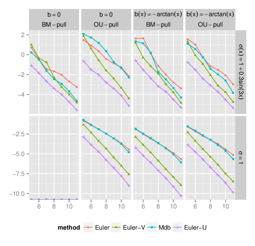
Figure 1: $\log_{2}(RMSE)$ of $I(\cdot)$ versus $\log_{2}(\text{nr of segments})$.

In the simulations, we simulated bridges starting in $u=0$ at time $0$ and ending in $v=3$ at time $T=1$. The results of the simulations are in figure 1 where we considered both $\sigma=1$ and $\sigma(x)=1+0.3\sin(3x)$. By definition, there is no error in the lower-left panel. From the simulation results we see that for various combined choices of drift, diffusion coefficient and pulling term, our approach performs best. We have run simulations with other values for $v$, $T$, $b$ and $\sigma$ leading qualitatively to the same conclusion.

The beneficial effect of the time change and scaling is further illustrated in the examples of Sections 7.1 and 7.2.

5.3 Order of convergence

Ideally, one would derive a result on the order of convergence of each of the discussed discretisation methods for approximating $I$. We feel that this is outside the scope of this paper. As noted in Papaspiliopoulos et al. (2013) (page 676): “Quantitative results on the relative efficiency of discretisation schemes are scarce in the literature.” In case $b=0$ and $\sigma$ is constant (which is the simplest case to consider), Papaspiliopoulos et al. (2013) show that the strong order of convergence of the Euler scheme is $O(\sqrt{\delta})$ at $T-\delta$. This shows that the usual higher $O(\delta)$ strong order (which holds for diffusions with additive noise) is lost due to the exploding behaviour of the drift. Along similar lines as in Papaspiliopoulos et al. (2013) one can prove that the strong order $\delta$ is maintained if the time-change and scaling is used. Admittedly, this is a rather weak result since (i) the case $b=0$ and $\sigma$ constant is very specific, (ii) the focus is on accurate evaluation of a path integral of the proposal bridge and not solely the process at specified points. The concept of strong order is not really needed here: we are interested in almost sure convergence of Euler approximation pathwise. Under local Lipschitz conditions on the drift and diffusion coefficients, the pathwise convergence rate of the Euler scheme coincides up to an arbitrarily small $\varepsilon>0$ with its strong convergence rate $1/2$ (Cf. Gyöngy (1998)). We expect the same pathwise convergence rate to hold for the integrals, when approximated using the proposed time-change and scaling. In this sense, it is not unexpected that the lower panel in figure 1 shows lines with slopes close to either $1/2$ (Euler, Mdb) or $1$ (Euler-V, Euler-U).

5.4 Motivation for the scaling

Consider the SDE for $\widetilde{X}$ as defined in equation (4.6). The corresponding fundamental matrix is given in equation (5.4). Define the process $\widetilde{X}^{\star}$ as the process $\widetilde{X}$, conditioned on $\widetilde{X}_{T}=v$. Then $\widetilde{X}^{\star}$ is a linear process itself with drift $\widetilde{b}^{\star}(t,x)=\widetilde{B}(t)x+\widetilde{\beta}(t)+\widetilde{a}(t)\widetilde{H}(t)(v(t)-x)$ and diffusion coefficient $\widetilde{\sigma}^{\star}(t)=\sigma(t)$. Denote the corresponding fundamental matrix by $F^{\star}$. Hence $F^{\star}$ satisfies

$$\frac{{\,\mathrm{d}}}{{\,\mathrm{d}}t}{F^{\star}}(t)=\left(\widetilde{B}(t)-\widetilde{a}(t)\widetilde{H}(t)\right)F^{\star}(t),\qquad F^{\star}(0)=\mathrm{I}.$$

Theorem 5.3.

Fix a nondecreasing differentiable mapping $\tau\,:\,[0,T]\to[0,\infty)$. If we define the scaling matrix $m$ by $m(s)=(T-s){F^{\star}}(\tau(s))^{-1}$. then the process $U$ defined by

$$U_{s}=m(s)\left[v(\tau(s))-X^{\circ}_{\tau(s)}\right]$$

(with $s\mapsto v(s)$ as defined in equation (5.3)) satisfies the SDE

$${\,\mathrm{d}}U_{s}=\left(-\frac{U_{s}}{T-s}-m\dot{\tau}\left[b(\tau,\Gamma)-\widetilde{b}(\tau,\Gamma)\right.\right.\\ \left.\left.+(a(\tau,\Gamma)-\widetilde{a}(\tau))\widetilde{H}(\tau)m^{-1}U_{s}\right]\right){\,\mathrm{d}}s-m\sqrt{\dot{\tau}}\sigma(\tau,\Gamma){\,\mathrm{d}}W_{s},$$

where $\Gamma\equiv\Gamma(s,U_{s})=v(\tau(s))-m(s)^{-1}U_{s}$. To lighten the notation we have written $\tau$, $\dot{\tau}$ and $m$ to denote $\tau(s)$, $\dot{\tau}(s)$ and $m(s)$ respectively.

The proof is deferred to the appendix (section B).

Corollary 5.4.

Let $\bar{U}_{t_{i}}$ denote the Euler approximation at time $t_{i}$ of $U$. If $a(t,x)\equiv a(T,v)=\widetilde{a}$ and $b(t,x)=\widetilde{b}(t,x)=\widetilde{B}(t)x+\widetilde{\beta}(t)$, then

$${\rm E}\mspace{-1.0mu}\left[U_{t_{i}}\mid U_{t_{i-1}}=u\right]={\rm E}\mspace{-1.0mu}\left[\bar{U}_{t_{i}}\mid\bar{U}_{t_{i-1}}=u\right].$$

Proof.

In this case

$${\,\mathrm{d}}U_{s}=-\frac{U_{s}}{T-s}{\,\mathrm{d}}s-m\sqrt{\dot{\tau}}\sigma(\tau,\Gamma){\,\mathrm{d}}W_{s}.$$

Hence

$${\rm E}\mspace{-1.0mu}\left[U_{t_{i}}\mid U_{t_{i-1}}=u\right]=\frac{T-t_{i}}{T-t_{i-1}}u.$$

It is easy to see that this coincides with ${\rm E}\mspace{-1.0mu}\left[\bar{U}_{t_{i}}\mid\bar{U}_{t_{i-1}}=u\right]$. ∎

This shows that if we use linear guided proposals and use the scaling matrix $m$ defined in theorem 5.3, then the Euler approximation of the process $U$ has the correct conditional expectation when $X$ itself is a linear process. Note that this is not necessarily the case without applying the scaling.

In case $\widetilde{\beta}=0$, $\widetilde{B}=0$ and $\widetilde{\sigma}(t)=\widetilde{\sigma}$, we have $F^{\star}(t)=\mathrm{I}/(T-t)$ and $m(s)=1/(T(T-s))\mathrm{I}$. This means that we should have $m(s)=O(1/(T-s))$ for $s\approx T$.

6 Computational costs and implementation

In this section we discuss the computational cost of using guided proposals. For comparison, we add the computational cost of Delyon-Hu type proposals. Here we only consider the cost of imputation by diffusion bridges (including the computation of their acceptance probabilities). Let

• $K$ denote the number of iterations of the data-augmentation algorithm;

• $M$ denote the number of segments for imputations (so $M+1$ is the number of discrete-time observations);

• $N$ denote the number of Euler-step applied to each segment.

The computational costs of simulating proposals are summarised in table 1. We give some elucidation on this table.

1. Applying guided proposals with $\widetilde{B}\equiv 0$ gives minor additional computations compared to Delyon-Hu type proposals. One merely needs to compute $\int_{t}^{T}\beta_{\theta}(s){\,\mathrm{d}}s$ on the whole augmented grid during all simulations. If $\beta$ does not depend on $\theta$ this computation needs to be carried out only once on the whole grid.

2. If $\widetilde{B}\not\equiv 0$, then simulation of $U$ as defined in equation (5.7) requires evaluation of both $\dot{v}$ and $J$, where $v$ and $J$ are defined in equations (5.3) and (5.8) respectively. As $\dot{v}(s)=\widetilde{B}(s)v(s)+\widetilde{\beta}(s)$, evaluating $\dot{v}$ requires evaluation of $v$. This in turn requires evaluation of matrix exponentials. For evaluating $J$, we first compute $\lambda$ as the solution to continuous time Lyapunov equation $B\lambda+\lambda B^{\prime}=-\widetilde{a}$. Using $\lambda$ we can evaluate $J$ using

   $$J(s)=z(s)\left(e^{-\widetilde{B}_{\theta}z(s)}\lambda e^{-\widetilde{B}_{\theta}^{\prime}z(s)}-\lambda\right)^{-1},$$

   where $z(s)=T-\tau(s)$. These functions need to be computed on the whole augmented grid in each iteration. In case $\widetilde{B}$ does not depend on $\theta$, both $J$ and $\dot{v}$ can be precomputed on a grid in advance to the MCMC-algorithm, preventing multiple expensive matrix exponential computations.

Besides simulation of the proposals, an acceptance probability needs to be computed. This requires evaluation of certain integrals of the proposal. A potential disadvantage of Delyon-Hu type proposals is that inverses appear. Moreover, stochastic integrals need to be approximated.

	$\int_{t}^{T}\beta_{\theta}{\,\mathrm{d}}s$	$\exp\left(sB\right)$	$B\lambda+\lambda B^{\prime}=\widetilde{a}$
Delyon-Hu	0	0	0
$\widetilde{b}(t,x)=\beta_{\theta}(t)$	$NMK$	0	0
$\widetilde{b}(t,x)=Bx+\beta_{\theta}(t)$	$NMK$	$N$	$M$
$\widetilde{b}(t,x)=B_{\theta}x+\beta_{\theta}(t)$	$NMK$	$NK$	$MK$

Table 1: Overview of computational cost for simulating proposals.

7 Examples

The source code of the examples is available online. It is written in the programming language Julia (Bezanson et al. (2012)).

7.1 Example for one-dimensional diffusion

In this section we discuss example 4.3. The goal is twofold: (i) to show that the proposed algorithm does not deteriorate when increasing the number of imputed points, (ii): to show that the discretisation scheme of section 5 reduces discretisation error.

We take the diffusion process with dynamics of (4.11). Assume that we observe $X$ at times points $t=0,0.3,0.6\dots,T=30$ and wish to estimate $(\alpha,\beta,\sigma)$. As true values we took $\alpha=-2,\beta=0$ and $\sigma=0.75$. For generating the discrete time data we simulated the process on $[0,T]$ at $400\,001$ equidistant time points using the Euler scheme and take a subsample.

For $\alpha$ and $\beta$ we chose apriori independently a ${\mathcal{N}}(0,\xi^{2})$-distribution with variance $\xi^{2}=5$. For $\log\sigma$ we used an uninformative flat prior. We applied algorithm 2 with $\rho=0$ in (3.8) with random walk proposals for $q(\sigma^{\circ}\mid\sigma)$ of the form $\log\sigma^{\circ}:=\log\sigma+u$ with $u\sim{\mathcal{U}}(-0.1,0.1)$.

We initialised the sampler with $\alpha=-0.1$, $\beta=-0.1$ and $\sigma=2$ and varied the number of imputed points over $m=10,100$ and $1000$. Acceptance rates for proposed bridges were in all cases between $94\%$ and $95\%$ and for $\sigma$ between $72\%$ and $73\%$.

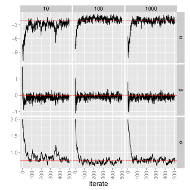
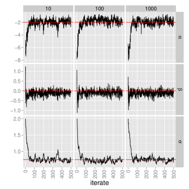
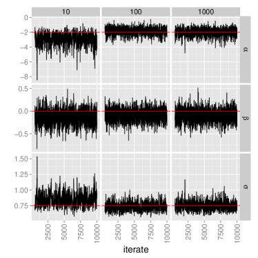
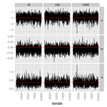
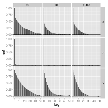
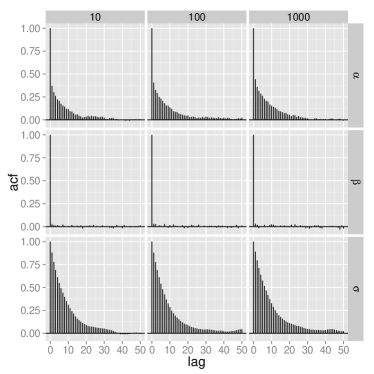
Figure 2: Panels comparing different numbers of imputed points ($m=10,100,1000$). Left: without time change. Right: with time change. Top: first 500 iterates. Middle: iterates 501-10.000. Bottom: ACF-plots based on iterates 501-10.000.

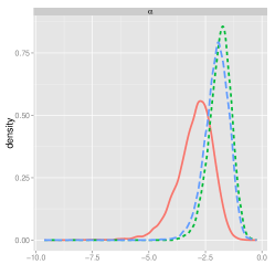
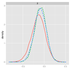
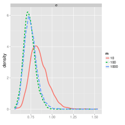
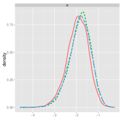
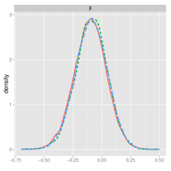
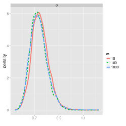
Figure 3: Kernel density estimates of the parameters based on iterates 501-10.000. Top: non time-changed. Bottom: time-changed. The bias from using only a small number of imputed points ($m=10$, red curve) is clearly smaller for the time changed process. For a high number of imputed points ($m=1000$, blue dashed curve) both methods agree.

Figures 2 and 3 illustrate the results of running the MCMC chain for 10.000 iterations using $m=10,100,1000$ imputed points respectively for each bridge (including endpoints), both with time change and without. Two things stand out: firstly, increasing the number of imputed points $m$ does not worsen the mixing of the chain and secondly the vastly reduced bias when using discretisation of $U$ (especially when $m$ is small).

7.2 FitzHugh-Nagumo model

The stochastic FitzHugh-Nagumo model for spike generation in squid axons is based on a two dimensional diffusion process with drift and diffusion coefficent parametrised as

$$b(x)=\begin{bmatrix}\vartheta_{1}(-x_{1}^{3}+x_{1}-x_{2}+1/2)\\ \vartheta_{2}x_{1}-x_{2}+\vartheta_{3}\end{bmatrix}\qquad\sigma=\begin{bmatrix}\gamma_{1}&0\\ 0&\gamma_{2}\end{bmatrix}.$$

The first coordinate $X^{(1)}$ represents the axon membrane potential and $X^{(2)}$ is a recovery variable. Parameter estimation for the FitzHugh-Nagumo model is discussed in Jensen et al. (2012) and extensively in the work of Jensen (2014). In this example we consider three type of proposals: the modified diffusion bridge (which is of Delyon-Hu type with $\lambda=0$), the modified diffusion bridge with random-walk type updates on the innovations and guided-proposals with random-walk type updates on the innovations. In both cases we took $\rho=0.5$ in equation (3.8). We used time-change guided proposals as in (5.5) with $\widetilde{\sigma}$ constant, $\widetilde{B}\equiv 0$ and $\widetilde{\beta}$ as in equation (4.10). This is a simple default choice. We discretise (5.7) as follows: suppose the current iterate is $U_{s}$. We have

$${\,\mathrm{d}}U_{s}=\frac{{\,\mathrm{d}}s}{T}(\widetilde{b}(\tau(s))-b(\tau(s),\Gamma(s,U_{s})))+{\,\mathrm{d}}R_{s}$$ (7.1)

with ${\,\mathrm{d}}R_{s}=(T-s)^{-1}\Big{(}\mathrm{I}-2aJ(s)\Big{)}U_{s}{\,\mathrm{d}}s-\sqrt{\frac{2}{T}}\frac{1}{\sqrt{T-s}}\sigma{\,\mathrm{d}}W_{s}$ (where we have used the relation $\dot{v}(s)=\widetilde{\beta}(s)$). Define

$$\bar{R}(h)=(T-s)^{-1}\Big{(}\mathrm{I}-2aJ(s)\Big{)}U_{s}-\sqrt{\frac{2}{T}}\frac{1}{\sqrt{T-s}}\sigma\frac{W_{s+h}-W_{s}}{h}.$$

To obtain an approximation $u(s+h)$ for $U_{s+h}$ we discretise the ordinary differential equation

$${\,\mathrm{d}}u(s)=\left(\frac{1}{T}\widetilde{b}(\tau(s))-\frac{1}{T}b(\tau(s),\Gamma(s,u(s)))+\bar{R}(h)\right){\,\mathrm{d}}s,\qquad u(s)=U_{s}$$

using the Runge-Kutta-4 method with step size $h$. We propose this discretisation scheme since by corollary 5.4, ${\rm E}\mspace{-1.0mu}\left[R_{s+h}-R_{s}\mid R_{s}\right]=h{\rm E}\mspace{-1.0mu}\left[\bar{R}(h)\mid R_{s}\right]$.

We simulated the process with parameters $\vartheta_{1}=1.4$, $\vartheta_{2}=1.5$, $\vartheta_{3}=10$, $\gamma_{1}=0.25,\gamma_{2}=0.2$ on the time interval from $0$ to $T=300$ using the Euler scheme with discretisation step $0.0004$ , starting in $[0\;1]^{\prime}$, retaining $400$ equidistant observations and the starting point. With these parameters this process presents a challenging estimation problem due to the strong nonlinear dynamics in the drift.

We chose independent centred Gaussian priors with variance $50$ for the parameters $\vartheta_{1},\vartheta_{2},\vartheta_{3}$ and a product $\operatorname{InvGamma}(0.002,0.002)$ prior on $(\gamma^{2}_{1},\gamma_{2}^{2})$.

We used Metropolis-Hastings steps for updating $\gamma_{i}$ by setting $\log\gamma_{i}^{\circ}=\log\gamma_{i}+0.02Z_{i}$ ($i=1,2$), where $Z_{i}\sim N(0,1)$. For $j=1,2,3$ we took $\vartheta_{j}^{\circ}=\vartheta_{j}+\nu_{j}Y_{j}$, with $Y_{j}$ independent Uniform random variables on $[-1,1]$, $\nu_{1}=\nu_{2}=0.03$ and $\nu_{3}=0.15$.

We estimated the joint posterior of unobserved path and parameters $\vartheta$, $\gamma$ using algorithm 1.

We ran the algorithm for the three different proposals with $m=10$ and $m=25$ and $m=100$. Each simulation was stopped after $1$ hour. The simulations were done on a computer equipped with 4 core Xeon CPU clocked at 3.40GHz with 30 GiB memory. In figure 4 trace-plots with respect to both computing time and iterate number for $\vartheta_{3}$ are shown for the three samplers when $m\in\{10,25,100\}$. While iterates for the guided-proposals are more costly, the algorithm with these proposals does reach the stationary region way faster than the two variants of the modified diffusion bridge, especially when $m=100$. However, solely examining trace-plots for the parameters can be misleading as illustrated by figure 5. Here, we plotted the average acceptance probability for bridge proposals (on a log10-scale) for the segments in between the $99$-th and $200$-th observations (the picture is representative for all segments). At certain segments the acceptance probabilities differ by several magnitudes. These segments correspond precisely to observations during an excursion from the meta-stable region. In these excursions the diffusion path follows closely the strong nonlinear drift dynamics, unlike in the meta-stable region. Small acceptance probabilities manifest themselves in slow convergence of the chain.

In addition we ran the algorithm for a longer time ($16$ hours) with $m=200$. In this case, we simply used the Euler-approximation for the time-changed guided proposals. Actually, the Runge-Kutta-4 method is due to the stiffness of the SDE and only necessary in case of few imputed points. Trace-plots for $\vartheta_{3}$ and $\gamma_{1}$ are shown in figure 6. The trace-plot of $\gamma_{1}$ against iteration number clearly shows that the guided proposals chain mixes better. The posterior means obtained by these methods were then considered to be the “true” posterior mean. These were used in computing the error values in table 2.

m = 10	RRSE	$\vartheta_{1}$	$\vartheta_{2}$	$\vartheta_{3}$	$\gamma_{1}$	$\gamma_{2}$	mESS	K
mdb-rw	0.3	0.96	0.95	0.75	0.94	0.94	598.4	88485
gp-tc	0.29	1.03	1.04	0.76	1.02	0.99	333.67	27366
mdb-ind	0.49	0.9	0.88	0.6	1.08	1.05	761.25	88685
m = 25	RRSE	$\vartheta_{1}$	$\vartheta_{2}$	$\vartheta_{3}$	$\gamma_{1}$	$\gamma_{2}$	mESS	K
mdb-rw	0.18	0.95	0.94	0.85	1.06	0.96	439.12	47576
gp-tc	0.1	1	1	0.91	1.05	0.99	177.78	12359
mdb-ind	0.42	0.91	0.89	0.65	1.16	1.09	505.77	47006
m = 100	RRSE	$\vartheta_{1}$	$\vartheta_{2}$	$\vartheta_{3}$	$\gamma_{1}$	$\gamma_{2}$	mESS	K
mdb-rw	0.2	0.94	0.93	0.84	1.09	0.99	216.48	14259
gp-tc	0.01	0.99	0.98	1.01	1.08	1.01	85.47	3365
mdb-ind	0.39	0.89	0.87	0.68	1.19	1.1	246.4	14441

Table 2: Estimation results FitzHugh-Nagumo model based on all iterates (no burn-in was considered). For each parameter we report its relative error with respect to the posterior mean obtained from the $16$-hour run with $m=200$ imputed points using the time-changed guided proposals. Furthermore, we report the Root Relative Squared Error (RRSE) and the multivariate Effective Sample Size (mESS) from Vats et al. (2015). $K$ is the total number of iterations executed within one hour.

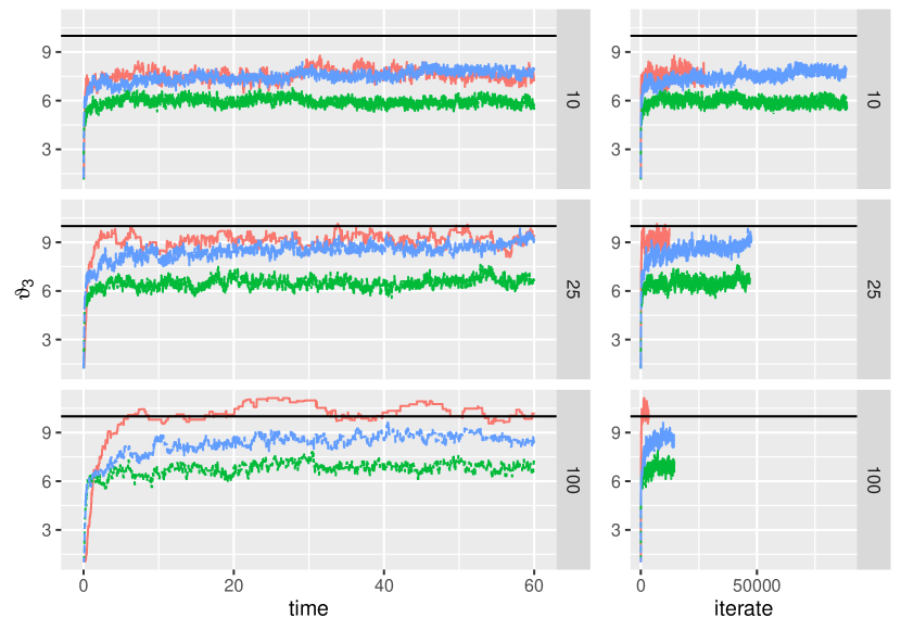
Figure 4: Trace-plots for $\vartheta_{3}$. Left: with respect to computing time in minutes. Right: with respect to iterate number. The three different panels correspond to $m=10$, $m=25$ and $m=100$. “gp-tc” for guided proposals time-changed; “mdb-rw” for random-walk type modified diffusion bridges; “mdb-rw” for modified diffusion bridges.

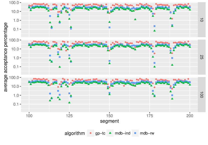
Figure 5: Average acceptance percentages for proposed bridges on segments $100$ up to $200$. The three different panels correspond to $m=10$, $m=25$ and $m=100$.

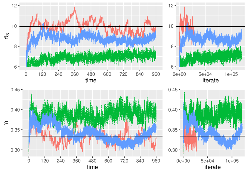
Figure 6: Trace-plots for $\vartheta_{3}$ and $\gamma_{1}$. Left: with respect to computing time in minutes. Right: with respect to iterate number. In all cases $m=200$. “gp-tc” is guided proposals time-changed; “mdb-rw” is random-walk type modified diffusion bridge; “mdb-rw” is modified diffusion bridge. The initial $735$ iterates of $\vartheta_{3}$ are smaller than $6$ and not shown.

Appendix A Proof of Lemma 5.2

For ease of notation we will write $\tau$ and $\dot{\tau}$ instead of $\tau(s)$ and $\dot{\tau}(s)$. If $X$ satisfies the SDE

$${\,\mathrm{d}}X_{s}=b(s,X_{s}){\,\mathrm{d}}s+\sigma(s,X_{s}){\,\mathrm{d}}\widetilde{W}_{s}$$

and we are given a smooth function $\tau=\tau(s)$, $\tau\colon[0,T)\to\mathbb{R}_{+}$ with positive derivative $\dot{\tau}$, then

$${\,\mathrm{d}}X_{\tau}=\dot{\tau}b(\tau,X_{\tau}){\,\mathrm{d}}s+\sqrt{\dot{\tau}}\sigma(\tau,X_{\tau}){\,\mathrm{d}}W_{s},$$ (A.1)

where $W$ is a different Brownian motion on the same probability space as $\widetilde{W}$.

Applying this to $X^{\circ}$ (defined in equation (3.3)) gives

$${\,\mathrm{d}}X^{\circ}_{\tau}=2(1-s/T)[b(\tau,X^{\circ}_{\tau})+a(\tau,X^{\circ}_{\tau})\widetilde{r}(\tau,X^{\circ}_{\tau})]{\,\mathrm{d}}s+\sqrt{2(1-s/T)}\sigma(\tau,X^{\circ}_{\tau}){\,\mathrm{d}}W_{s}$$

by Itō’s formula

$${\,\mathrm{d}}U_{s} ={\,\mathrm{d}}\left(\frac{v(\tau)-X^{\circ}_{\tau}}{T-s}\right)$$

$$=\frac{2}{T}\dot{v}(\tau){\,\mathrm{d}}s+\frac{v(\tau)}{(T-s)^{2}}{\,\mathrm{d}}s-\frac{X^{\circ}_{\tau}}{(T-s)^{2}}{\,\mathrm{d}}s$$

$$\qquad\qquad-\frac{2}{T}[b(\tau,X^{\circ}_{\tau})+a(\tau,X^{\circ}_{\tau})\widetilde{r}(\tau,X^{\circ}_{\tau})]{\,\mathrm{d}}s-\frac{\sqrt{2/T}}{\sqrt{T-s}}\sigma(\tau,X^{\circ}_{\tau}){\,\mathrm{d}}W_{s}$$

$$=\frac{2}{T}\dot{v}(\tau){\,\mathrm{d}}s+\frac{U_{s}}{T-s}{\,\mathrm{d}}s-\frac{2}{T}[b(\tau,X^{\circ}_{\tau})+a(\tau,X^{\circ}_{\tau})\widetilde{r}(\tau,X^{\circ}_{\tau})]{\,\mathrm{d}}s$$

$$\qquad\qquad-\frac{\sqrt{2/T}}{\sqrt{T-s}}\sigma(\tau,X^{\circ}_{\tau}){\,\mathrm{d}}W_{s}.$$

By equation (5.2),

$$\widetilde{r}(\tau,X^{\circ}_{\tau})=\widetilde{H}(\tau)(v(\tau)-X^{\circ}_{\tau})=\widetilde{H}(\tau)(T-s)U_{s}=J(s)\frac{T}{T-s}U_{s}.$$

The result now follows from substituting this expression and using the relation $X^{\circ}_{\tau(s)}=\Gamma(s,U_{s})$ (see (5.6)).

The statement on $J$ is a consequence of $\widetilde{a}(s)J(s)=\widetilde{H}(\tau(s))(T-\tau(s))$ together with $\lim_{t\to T}\widetilde{H}(t)(T-t)=\widetilde{a}^{-1}$ (see (Schauer et al., 2016, Lemma 8)).

The expression for the integral follows upon the substitution $s:=\tau(s)$ and using relation (5.2).

Appendix B Proof of Theorem 5.3

Proof.

By straightforward calculus, the process $U$ satisfies a SDE with drift coefficient

$$m\dot{v}(\tau)\dot{\tau}+\dot{m}m^{-1}U_{s}-m\dot{\tau}\left[b(\tau,\Gamma)+a(\tau,\Gamma)\widetilde{H}(\tau)m^{-1}U_{s}\right]$$

and diffusion coefficient as given in the theorem. We can rewrite the drift coefficient using specific properties of $m$.

For the first term in the drift, note that

$$\widetilde{b}(\tau,\Gamma)=\widetilde{B}(\tau)\left(v(\tau)-m^{-1}U_{s}\right)+\widetilde{\beta}(\tau)=\dot{v}(\tau)-\widetilde{B}(\tau)m^{-1}U_{s},$$

where we have used the relation $\dot{v}(s)=\widetilde{B}(s)v(s)+\widetilde{\beta}(s)$ at the second equality. Multiplying by $m\dot{\tau}$ we get

$$m\dot{\tau}\dot{v}(\tau)=m\dot{\tau}\widetilde{b}(\tau,\Gamma)+m\dot{\tau}\widetilde{B}(\tau)m^{-1}U_{s}.$$ (B.1)

Next, we rewrite the second term appearing in the drift. Using $\mathrm{d}{A}^{-1}/\mathrm{d}t=-{A}^{-1}\left(\mathrm{d}{A}/\mathrm{d}t\right){A}^{-1}$ for an invertible matrix $A$, we obtain that

$$\dot{m}m^{-1}=-(T-s)^{-1}\mathrm{I}-\dot{\tau}\left(\widetilde{B}(\tau)-\widetilde{a}(\tau)\widetilde{H}(\tau)\right).$$ (B.2)

Substituting (B.1) and (B.2) into the drift and reordering terms shows that the drift of $U$ equals

$$-(T-s)^{-1}U_{s}-m\dot{\tau}\left(b(\tau,\Gamma)-\widetilde{b}(\tau,\Gamma)\right)\\ +m\dot{\tau}\left(\widetilde{B}(\tau)-a(\tau,\Gamma)\widetilde{H}(\tau)\right)m^{-1}U_{s}-\dot{\tau}\left(\widetilde{B}(\tau)-\widetilde{a}(\tau)\widetilde{H}(\tau)\right)U_{s}.$$

This can be simplified to the form given in the theorem by using that

$$\widetilde{B}(\tau)-\widetilde{a}(\tau)\widetilde{H}(\tau)=m\left(\widetilde{B}(\tau)-\widetilde{a}(\tau)\widetilde{H}(\tau)\right)m^{-1}$$

which follows from the defining relation of $F^{\star}$. ∎

References

• Beskos et al. (2006) Beskos, A., Papaspiliopoulos, O., Roberts, G. O. and Fearnhead, P. (2006). Exact and computationally efficient likelihood-based estimation for discretely observed diffusion processes. J. R. Stat. Soc. Ser. B Stat. Methodol. 68(3), 333–382. With discussions and a reply by the authors.
• Bezanson et al. (2012) Bezanson, J., Karpinski, S., Shah, V. B. and Edelman, A. (2012). Julia: A fast dynamic language for technical computing. CoRR abs/1209.5145.
• Bladt and Sørensen (2014) Bladt, M. and Sørensen, M. (2014). Simple simulation of diffusion bridges with application to likelihood inference for diffusions. Bernoulli 20(2), 645–675.
• Bladt and Sørensen (2015) Bladt, M. and Sørensen, M. (2015). Simulation of multivariate diffusion bridges. To appear in Journal of the Royal Statistical Society, series B .
• Chib et al. (2004) Chib, S., Pitt, M. K. and Shephard, N. (2004). Likelihood based inference for diffusion driven models. Economics Papers 2004-W20, Economics Group, Nuffield College, University of Oxford.
• Clark (1990) Clark, J. M. C. (1990). The simulation of pinned diffusions. In Decision and Control, 1990., Proceedings of the 29th IEEE Conference on, pp. 1418–1420. IEEE.
• Delyon and Hu (2006) Delyon, B. and Hu, Y. (2006). Simulation of conditioned diffusion and application to parameter estimation. Stochastic Processes and their Applications 116(11), 1660 – 1675.
• Durham and Gallant (2002) Durham, G. B. and Gallant, A. R. (2002). Numerical techniques for maximum likelihood estimation of continuous-time diffusion processes. J. Bus. Econom. Statist. 20(3), 297–338. With comments and a reply by the authors.
• Elerian et al. (2001) Elerian, O., Chib, S. and Shephard, N. (2001). Likelihood inference for discretely observed nonlinear diffusions. Econometrica 69(4), 959–993.
• Eraker (2001) Eraker, B. (2001). MCMC analysis of diffusion models with application to finance. J. Bus. Econom. Statist. 19(2), 177–191.
• Fuchs (2013) Fuchs, C. (2013). Inference for diffusion processes. Springer, Heidelberg. With applications in life sciences, With a foreword by Ludwig Fahrmeir.
• Golightly and Wilkinson (2010) Golightly, A. and Wilkinson, D. J. (2010). Learning and Inference in Computational Systems Biology, chapter Markov chain Monte Carlo algorithms for SDE parameter estimation, pp. 253–276. MIT Press.
• Gugushvili and Spreij (2012) Gugushvili, S. and Spreij, P. (2012). Parametric inference for stochastic differential equations: a smooth and match approach. ALEA Lat. Am. J. Probab. Math. Stat. 9(2), 609–635.
• Gyöngy (1998) Gyöngy, I. (1998). A note on Euler’s approximations. Potential Anal. 8(3), 205–216.
• Jensen et al. (2012) Jensen, A. C., Ditlevsen, S., Kessler, M. and Papaspiliopoulos, O. (2012). Markov chain Monte Carlo approach to parameter estimation in the FitzHugh-Nagumo model. Phys. Rev. E 86, 041114.
• Jensen (2014) Jensen, C., Anders (2014). Statistical Inference for Partially Observed Diffusion Processes. Ph.d. Thesis University of Copenhagen.
• Khasminskii and Klebaner (2001) Khasminskii, R. Z. and Klebaner, F. C. (2001). Long term behavior of solutions of the Lotka-Volterra system under small random perturbations. Ann. Appl. Probab. 11(3), 952–963.
• Küchler and Sørensen (1997) Küchler, U. and Sørensen, M. (1997). Exponential families of stochastic processes. Springer Series in Statistics. Springer-Verlag, New York.
• Lin et al. (2010) Lin, M., Chen, R. and Mykland, P. (2010). On generating Monte Carlo samples of continuous diffusion bridges. J. Amer. Statist. Assoc. 105(490), 820–838.
• Papaspiliopoulos and Roberts (2012) Papaspiliopoulos, O. and Roberts, G. (2012). Importance sampling techniques for estimation of diffusion models. In Statistical Methods for Stochastic Differential Equations, Monographs on Statistics and Applied Probability, p. 311–337. Chapman and Hall.
• Papaspiliopoulos et al. (2003) Papaspiliopoulos, O., Roberts, G. O. and Sköld, M. (2003). Non-centered parameterizations for hierarchical models and data augmentation. In Bayesian statistics, 7 (Tenerife, 2002), pp. 307–326. Oxford Univ. Press, New York. With a discussion by Alan E. Gelfand, Ole F. Christensen and Darren J. Wilkinson, and a reply by the authors.
• Papaspiliopoulos et al. (2013) Papaspiliopoulos, O., Roberts, G. O. and Stramer, O. (2013). Data Augmentation for Diffusions. J. Comput. Graph. Statist. 22(3), 665–688.
• Pedersen (1995) Pedersen, A. R. (1995). Consistency and asymptotic normality of an approximate maximum likelihood estimator for discretely observed diffusion processes. Bernoulli 1(3), 257–279.
• Roberts and Stramer (2001) Roberts, G. O. and Stramer, O. (2001). On inference for partially observed nonlinear diffusion models using the Metropolis-Hastings algorithm. Biometrika 88(3), 603–621.
• Rogers and Williams (2000) Rogers, L. C. G. and Williams, D. (2000). Diffusions, Markov processes, and martingales. Vol. 2. Cambridge Mathematical Library. Cambridge University Press, Cambridge. Itô calculus, Reprint of the second (1994) edition.
• Rosenthal (2011) Rosenthal, J. S. (2011). Handbook of Markov Chain Monte Carlo (Chapman & Hall/CRC Handbooks of Modern Statistical Methods), chapter Optimal proposal distributions and adaptive MCMC. Chapman and Hall/CRC, 1 edition.
• Schauer et al. (2016) Schauer, M., Van der Meulen, F. H. and Van Zanten, J. H. (2016). Guided proposals for simulating multi-dimensional diffusion bridges. Accepted for publication in Bernoulli. ArXiv e-prints 1311.3606 .
• Sermaidis et al. (2013) Sermaidis, G., Papaspiliopoulos, O., Roberts, G. O., Beskos, A. and Fearnhead, P. (2013). Markov chain Monte Carlo for exact inference for diffusions. Scand. J. Stat. 40(2), 294–321.
• Sørensen (2004) Sørensen, H. (2004). Parametric Inference for Diffusion Processes Observed at Discrete Points in Time: a Survey. Internat. Statist. Rev. 72, 337–354.
• Steiner and Gander (1999) Steiner, A. and Gander, M. J. (1999). Parametrische lösungen der räuber-beute-gleichungen im vergleich. Il Volterriano (7), 32–44.
• Stramer and Bognar (2011) Stramer, O. and Bognar, M. (2011). Bayesian inference for irreducible diffusion processes using the pseudo-marginal approach. Bayesian Anal. 6(2), 231–258.
• Tierney (1998) Tierney, L. (1998). A note on metropolis-hastings kernels for general state spaces. Ann. Appl. Probab. 8(1), 1–9.
• van der Meulen and Schauer (2016) van der Meulen, F. and Schauer, M. (2016). Bayesian estimation of incompletely observed diffusions. ArXiv e-prints .
• Van der Meulen et al. (2014) Van der Meulen, F. H., Schauer, M. and Van Zanten, J. H. (2014). Reversible jump MCMC for nonparametric drift estimation for diffusion processes. Comput. Statist. Data Anal. 71, 615–632.
• Van der Meulen and Van Zanten (2013) Van der Meulen, F. H. and Van Zanten, J. H. (2013). Consistent nonparametric Bayesian inference for discretely observed scalar diffusions. Bernoulli 19(1), 44–63.
• Van Zanten (2013) Van Zanten, J. H. (2013). Nonparametric bayesian methods for one-dimensional diffusion models. Mathematical biosciences 243(2), 215–222.
• Vats et al. (2015) Vats, D., Flegal, J. M. and Jones, G. L. (2015). Multivariate Output Analysis for Markov chain Monte Carlo. ArXiv e-prints .
• Whitaker et al. (2015) Whitaker, G. A., Golightly, A., Boys, R. J. and Sherlock, C. (2015). Improved bridge constructs for stochastic differential equations. ArXiv eprints .