Deflected propagation of a coronal mass ejection from the corona to interplanetary space

Abstract

Among various factors affecting the space weather effects of a coronal mass ejection (CME), its propagation trajectory in the interplanetary space is an important one determining whether and when the CME will hit the Earth. Many direct observations have revealed that a CME may not propagate along a straight trajectory in the corona, but whether or not a CME also experiences a deflected propagation in the interplanetary space is a question, which has never been fully answered. Here by investigating the propagation process of an isolated CME from the corona to interplanetary space during 2008 September 12 – 19, we present solid evidence that the CME was deflected not only in the corona but also in the interplanetary space. The deflection angle in the interplanetary space is more than $20^{\circ}$ toward the west, resulting a significant change in the probability the CME encounters the Earth. A further modeling and simulation-based analysis suggest that the cause of the deflection in the interplanetary space is the interaction between the CME and the solar wind, which is different from that happening in the corona.

1 Introduction

Coronal mass ejections (CMEs) that originate from solar source regions facing Earth are thought to be one of the main drivers of hazardous space weather. Such CMEs usually appear like a halo in a coronagraph. However, not all of such halo CMEs hit the Earth. Only about 60%–70% of front-side halo CMEs are found to be associated with an ejecta near the Earth, and the fraction is even smaller, $\sim 50\%$, for geoeffective front-side CMEs [e.g., Webb et al., 1996, 2001; Cane et al., 1998; Plunkett et al., 2001; Wang et al., 2002; Berdichevsky et al., 2002; Yermolaev et al., 2005]. On the other hand, CMEs originating from solar limb are possible to hit the Earth [e.g., Webb et al., 2000; Zhang et al., 2003; Cid et al., 2012]. Such events might cause so called ‘problem storms’, which cannot be found any associated on-disk CMEs [Webb et al., 2000; Schwenn et al., 2005; Zhang et al., 2007]. Statistical studies suggested that the association of ejecta to CMEs is about 60% [e.g., Lindsay et al., 1999; Cane et al., 2000; Cane and Richardson, 2003].

For problem storms, there are several possible explanations. One of them is that such storms are caused by CMEs with a large longitudinal extension, which could sweep through the Earth even if originating far from the disk center [Webb et al., 2000; Zhang et al., 2003]. The existence of stealth CMEs, which have been recently observed by the Solar-Terrestrial Relationship Observatories (STEREO, Kaiser et al. 2008), is another hypothesis. Such CMEs do not leave any footprints behind them in EUV observations [Robbrecht et al., 2009] though they may face to the observer. Statistical studies suggested that stealth CMEs are not a rare phenomenon, but may correspond to one third of all front-side CMEs [Ma et al., 2010; Wang et al., 2011]. Both of the above explanations could explain the problem storms but cannot explain why some CMEs originating from the solar disk center miss the Earth.

A promising explanation is that CMEs may be deflected during their propagation in the corona and interplanetary space. CME-CME interaction is a cause of CME deflection [Wang et al., 2011; Shen et al., 2012; Lugaz et al., 2012]. The deflected propagation angle could be ten degrees or even larger. More interestingly, observations imply that, even if there was only one CME, it could be deflected by the background solar wind and magnetic field. The deflection of isolated CMEs in the plane-of-sky in corona was reported since 1986 [MacQueen et al., 1986], and has been studied by many researchers [e.g., Gopalswamy et al., 2003, 2004, 2009; Cremades and Bothmer, 2004; Cremades et al., 2006; Wang et al., 2011; Lugaz et al., 2011; Kahler et al., 2012; Zuccarello et al., 2012; Yang et al., 2012; DeForest et al., 2013; Zhou and Feng, 2013]. By using STEREO data, it is found that the CME deflection in corona could be more than $20^{\circ}$, and appear to be controlled by the gradient of the corona magnetic energy density [Shen et al., 2011a; Gui et al., 2011].

Whether or not an isolated CME could be also deflected in the interplanetary space is an open question, because the state of interplanetary space in some sense is much different from that of the corona. In the corona, the magnetic field is dominant, and the solar wind has not been well developed; whereas in the interplanetary space, the solar wind becomes dominant, as magnetic fields decrease with distance and the solar wind has fully accelerated.

The idea of CME deflection in interplanetary space was first proposed by Wang et al. [2002] through a statistical study, and then developed in their follow-up works [Wang et al., 2004, 2006]. For a CME faster than the ambient solar wind, the interplanetary magnetic field will be piled up ahead of the CME and cause an eastward deflection; while for a CME slower than the solar wind, the magnetic field will accumulate behind the CME and cause a westward deflection [see Fig.4 of Wang et al., 2004]. The deflection angle could reach tens degrees. But the direct evidence of such a deflection has rarely been reported. Some recent case studies linking remote-sensing and in-situ data indirectly suggested that CMEs are possible to be deflected in interplanetary space [e.g. Kilpua et al., 2009; Rodriguez et al., 2011; Isavnin et al., 2013]. With the aid of triangulation method, the propagation direction of CMEs in the heliosphere was investigated by Lugaz [2010] based on STEREO observations. He found that 6 out of 13 CMEs perhaps experienced a deflected propagation with the deflection angle larger than $20^{\circ}$, and both eastward and westward deflections exist. That previous work was focused on the development of new analysis techniques, therefore, the precise deflection process and its possible cause was not analyzed.

In this study, we present the first detailed analysis of the deflection of an isolated CME during its heliospheric propagation. We focus on a CME which occurred on 2008 September 12 and study its trajectory as well as the physical causes and mechanisms for the observed deflection. The observations of this event will be presented in the next section. In Sec. 3, by applying a variety of models, we will study the propagation of the CME, including the evolution of its velocity and direction. We draw conclusions in section 4 and discuss our results in term of physical causes of CME deflection in section 5.

2 Observations

2.1 Instruments and data

The imaging data used in the following analysis are from the Large Angle and Spectrometric Coronagraph (LASCO, Brueckner et al. 1995) onboard SOHO spacecraft and the Sun Earth Connection Coronal and Heliospheric Investigation (SECCHI) suites [Howard et al., 2008] onboard both STEREO-A (STA) and STEREO-B (STB) spacecraft. The in-situ data of interplanetary magnetic field and solar wind plasma at 1 AU are from IMPACT [Acuña et al., 2008] and PLASTIC [Galvin et al., 2008] instruments onboard STA and STB spacecraft and MFI [Lepping et al., 1995], SWE [Ogilvie et al., 1995] and 3DP [Lin et al., 1995] instruments onboard Wind Spacecraft. SOHO and Wind is located at the first Lagrange point of the Sun-Earth system, and the STEREO twin spacecraft fly in Earth’s orbit with an increasing separation to the Earth. The positions of STA and STB in HEE coordinates at the beginning of 2008 September 13 are plotted in Figure 1. At that time, STA is separated away from the Earth by about $39^{\circ}$, and STB by about $34^{\circ}$. The LASCO instrument carries two working cameras, C2 and C3, that covering the corona from 2.0 – 30 $R_{S}$. In SECCHI suites, there are cameras, COR1, COR2, HI1 and HI2, monitoring the corona and interplanetary space from 1.4 $R_{S}$ to beyond 1 AU. These imagers provide seamless observations of the kinematic evolution of a CME from multiple angles of views.

Figure 1: Positions of STA and STB relative to the Earth near which SOHO locates at the beginning of September 13. The red arrow denotes the initial propagation direction of the CME derived by GCS model. The blue circles indicate the propagation direction of the CME from out corona to interplanetary space, which are inferred from STEREO imaging data by HM triangulation method. The curved path formed by the blue circles suggests that the CME experienced a deflection process.

2.2 Imaging observations

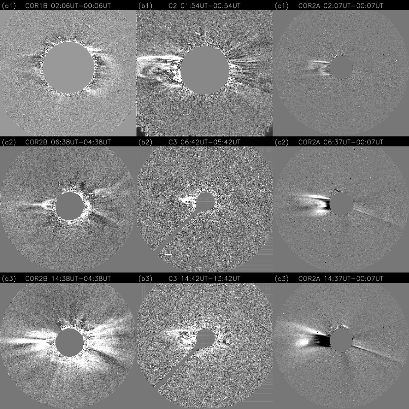
Figure 2: Snapshots of the CME taken by STB/COR (panel a), SOHO/LASCO (panel b) and STA/COR (panel c) on September 13. In both views of SOHO and STA, the CME looks like a east-limb event. But in the view of STB, it is a partial halo CME. Three movies generated from difference images have been attached in the online material to show the propagation of the CME viewed by SOHO, STA and STB, respectively.

The CME is a slow one as observed by STEREO and SOHO spacecraft (see Fig. 2, and associated movies). It roughly traveled in the ecliptic plane. In both the views of STA and SOHO, the CME looks like an east-limb event. Due to data gap, its first appearance in the field of view (FOV) of STA/COR1 is not clear, but must be before 15:00 UT on September 12, when the CME was already in the FOV of COR2. SOHO/LASCO C2 camera also captured an eastward CME starting at 15:30 UT, and 8 hours later, the CME appeared in the FOV of LASCO C3. Differently, in the view of STB, the CME presented a halo shape with main part expanding toward the west. It appeared in the FOV of STB/COR1 at about 19:38 UT on September 12, and emerged into the FOV of STB/COR2 about 9 hours later. Since it is a very slow CME, the CME fully developed into the FOVs of all the three coronagraphs around the beginning of September 13. Thus we just focus on the dynamic evolution of the CME since that time.

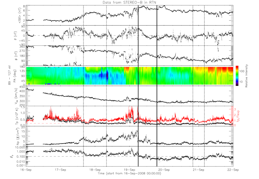
Figure 3: Interplanetary magnetic field and solar wind plasma data at 1 AU from in-situ instruments on board STB. The panels from the top to bottom are the magnetic field strength ($<|B|>$), elevation ($\theta$) and azimuthal ($\phi$) angles of the magnetic field direction, the electron pitch-angle (PA), the solar wind bulk speed ($v_{sw}$), the proton temperature ($T_{p}$), number density ($N_{p}$) and beta ($\beta$). The red curve in the 7th panel is the ratio of proton temperature to the expected proton temperature ($T_{exp}$), which is calculated based on the empirical formula by Lopez and Freeman [1986].

The CME appears as an east-limb event for both STA and SOHO. Considering the positions of STA and SOHO (Fig.1), it suggests that the initial CME direction of propagation, i.e., within 15 $R_{S}$, is on the east-side of the Sun-Earth line. For STB, the CME obviously inclined to the west, suggesting that the CME initial direction must be on the west-side of the Sun-STB line. Furthermore, considering that the CME looks more likely halo in the view of STB than in the view of SOHO, we may conclude that the initial propagation direction of the CME is located between the Sun-Earth line and the Sun-STB line and much closer to the later. So far, we have the first impression that the CME will encounter STB with its main body and sweep the Earth with its flank. To verify this, we check in-situ measurements from STA, STB and Wind.

2.3 In-situ observations

According to the coronagraph observations, we find that the initial speed of the CME is slower than 300 km s^-1. Even if the acceleration by the solar wind is taken into account, its average transit speed will not be larger than 500 km s^-1, which is higher than the typical value for the background solar wind speed. Thus it is expected that the interplanetary counterpart of the CME should be observed at 1 AU at least three days later. We examine the in-situ data from STA, STB and Wind spacecraft for 6 days starting from September 16. The parameters of interplanetary magnetic field and solar wind plasma during this period at three observational points are presented in Figure 3 through 5.

In Wind data, we can identify one and only one interplanetary CME during September 17 – 18 (see the shadow region in Fig.4), which is a magnetic cloud (MC) following, e.g., Burlaga et al. [1981]’s definition. Its front boundary is at about 04:20 UT on September 17 and the rear boundary at about 08:00 UT on the next day. All the MC signatures are very clear, which basically include (1) the enhanced magnetic field strength, (2) large and smooth rotation of magnetic field direction, (3) declining profile of solar wind velocity, (4) bi-directional streaming of supra-thermal electrons, (5) low proton temperature and (6) low proton $\beta$ ($<0.1$ generally) [e.g., Burlaga et al., 1981; Gosling et al., 1987; Lepping et al., 1990; Farrugia et al., 1993; Richardson and Cane, 1995]. The average speed of solar wind during the MC is about 415 km s^-1, suggesting the corresponding CME lifting off from the Sun around the beginning of September 13. Particularly, the STEREO imaging data show that there are no other CMEs directing to the Earth within 2 days before and after the CME. Thus it is conclusive that the MC observed by Wind is the interplanetary counterpart of the CME of interest.

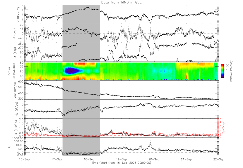
Figure 4: Same as Fig. 3 but from in-situ instruments on board Wind. The shadow region indicates an MC.

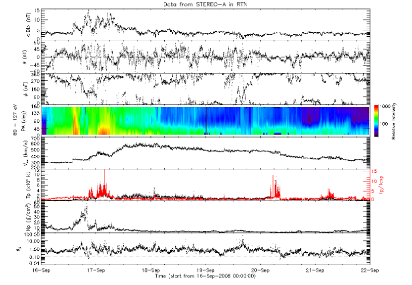
Figure 5: Same as Fig. 5 but from in-situ instruments on board STA.

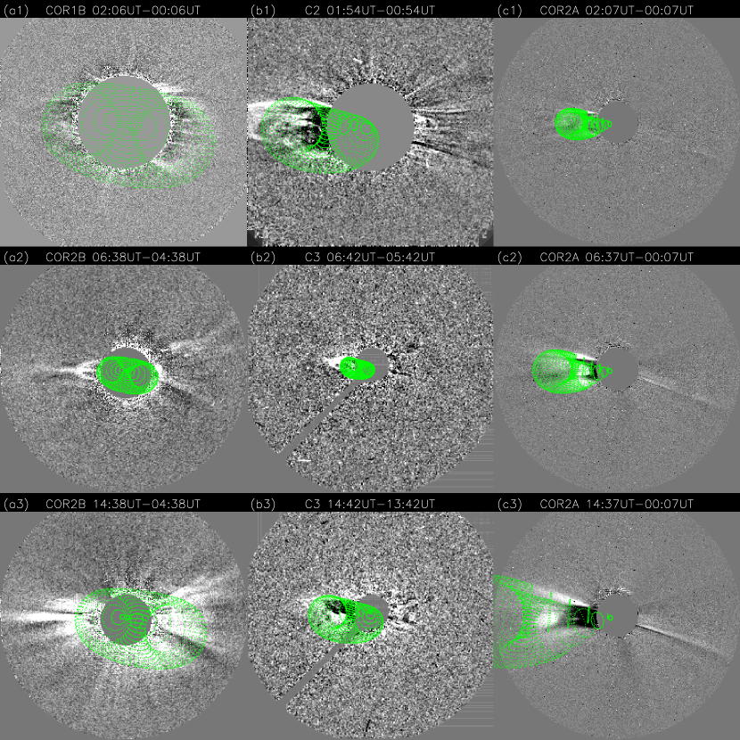
Figure 6: Coronagraph images showing the results of GCS model. The panels are the same as those in Fig. 2 but with flux rope meshes superimposed.

During the same period, STB did not capture any region with clear signatures of an MC, but it is possible to identify several MC-like or non-MC ejecta, e.g., the intervals between September 17 16:00 UT and September 18 08:00 UT, between September 19 06:00 UT and 19:00 UT, and between September 20 20:00 UT and September 21 04:00 UT (as indicated by vertical lines in Fig.3). None of them satisfies all the previously-mentioned six signatures of a typical MC. In the the first interval, there are only two signatures satisfied, i.e., the magnetic field is stronger than that of ambient solar wind and solar wind speed is declined. The second interval matches the most signatures, including smooth rotation of magnetic field vector, declining solar wind speed, bi-directional streaming of electrons and low proton $\beta$, but does not have significantly enhanced magnetic field and low proton temperature. The third interval also satisfies only two signatures, which are smooth rotation of magnetic field vector and low proton $\beta$. Considering that there was no other CME roughly toward STB in the week starting from September 12, we choose the ejecta in the second interval, which has the most signatures of an MC, as the counterpart of the CME of interest. This ejecta lost some signature of an MC is probably because the CME’s flank glanced over STB. The CME totally missed STA, as the STA data shows typical solar wind at all times except during the period from September 16 14:00 UT to September 17 12:00 UT, during which a corotating interaction region (CIR) was formed between a high speed solar wind stream and a low speed solar wind stream (Fig.5).

One may notice that the CME’s arrival at STB is about 2 days later than that at Wind. Such a long delay could be attributed to the curved front of the CME. A more detailed discussion on this issue will be given in Sec.4. The analysis of imaging data about the CME propagation in the corona has suggested that the CME’s main body should pass over STB and its flank glanced over the Earth, but the in-situ data from multiple points at 1 AU reveal that the fact is reversed, the CME’s main body passed through the Earth and its flank may have glanced over STB. This result suggests that the CME be deflected during its journey from the corona to 1 AU.

3 Propagation process

3.1 In corona

CMEs are believed to have a flux rope topology [e.g., Vourlidas et al., 2013]. Thus, the kinematic process of the CME is studied by applying a forwarding modeling with the aid of GCS model [Thernisien et al., 2009; Thernisien, 2011], which assumes that a CME has a flux-rope shape and expands self-similarly. It uses six free parameters to shape the flux rope, which are equivalent to height or heliocentric distance of the leading edge, latitude and longitude of the propagation direction, face-on and edge-on angular widths and tilt angle of the main axis of the flux rope. We get these parameters of a CME by fitting the GCS model to the observed outlines of a CME viewed from all the angles of views of SOHO, STA and STB. This model has been successfully applied to numerous CME events to study the deflected propagation of CMEs by Gui et al. [2011]. One may refer to the above references and therein for more details.

Figure 6 shows the CME with modeled flux rope superposed. In our fitting procedure, the face-on and edge-on widths and tilt angle are fitted as constants to reduce the degree of freedom. They are ${78^{\circ}}_{-18^{\circ}}^{+34^{\circ}}$, ${17^{\circ}}_{-5^{\circ}}^{+8^{\circ}}$ and $-11^{\circ}\pm 22^{\circ}$, respectively. The errors are estimated following the method by Thernisien et al. [2009], each of which will cause the 10% decrease of the best fit. With this configuration, the longitudinal extent of the CME in the ecliptic plane is estimated to be about $60^{\circ}$. The other three parameters are all time- or distance-dependent as shown in Figure 7. The errors in the distance, latitude and longitude are about $0.5R_{S}$, $2^{\circ}$ and $5^{\circ}$, respectively.

Since the GCS model requires that the CME is clearly visible in both images from STA and STB, the first result is obtained for time at 01:37 UT on September 13, when the CME’s leading edge already reached $7.1R_{S}$. At that time, the propagation direction of the CME is about $0.5^{\circ}$ in latitude and $-32^{\circ}$ in longitude in the heliocentric coordinates, i.e., about $2^{\circ}$ on the west of the Sun-STB line. The result is in agreement with our previous estimate of the CME initial propagation direction in Sec.2.2. Furthermore, we have tested the goodness-of-fit by assuming the CME propagated along the Sun-Earth line, which means that the CME was not deflected in interplanetary space. But the fitting result becomes much worse.

During the next 13 hours, the CME traveled from $7.1R_{S}$ to $22R_{S}$ with an average velocity of about 213 km s^-1. It experienced an acceleration process. The acceleration is about 5.8 m s^-2. During the period, the latitude of the CME direction did not change, but the longitude monotonically increased from $-32^{\circ}$ to $-25^{\circ}$. The CME was deflected toward the west by about $7^{\circ}$ in the corona. At 15:00 UT when the CME was $22R_{S}$ away from the Sun, the CME speed was accelerated to 353 km s^-1, and its propagation direction was changed to $9^{\circ}$ on the west of the Sun-STB line or $25^{\circ}$ on the east of the Sun-Earth line. The CME main body still tends to hit STB rather than the Earth, which is inconsistent with the in-situ observations presented in the last section. Thus the CME should be continuously deflected in interplanetary space.

Figure 7: De-projected position of the CME’s leading edge derived by GCS model. The errors in distance, latitude and longitude are about $0.5R_{S}$, $2^{\circ}$ and $5^{\circ}$, respectively. A systematically westward deflection is well revealed in the lower panel.

3.2 In interplanetary space

In order to track the CME in interplanetary space, an elongation-time map, known as J-map [Davies et al., 2009], is used. Figure 8 and 9 show the J-maps constructed based on the imaging data from COR2, HI1 and HI2 imagers onboard STA and STB by placing a slice along ecliptic plane. They provide the information from the corona to 1 AU. Any stripes with a positive slope in a J-map indicate a featured element moving away from the Sun. By comparing the stripes in the J-maps with the CME features in the images from COR2 and HI1, we may locate which one corresponds to the track of the CME’s leading edge in the FOVs of COR2 and HI1 in both J-maps, and then follow the track into the FOV of HI2 in the J-maps (as marked by blue diamonds). Since the CME’s leading edge appears weaker and more diffusive with increasing elongation angle, we set a reasonable error of about $\pm 5\%$ of elongation angle for the measurements. As seen in Figure 8 and 9, the error bars can cover the width of the diffusing tracks.

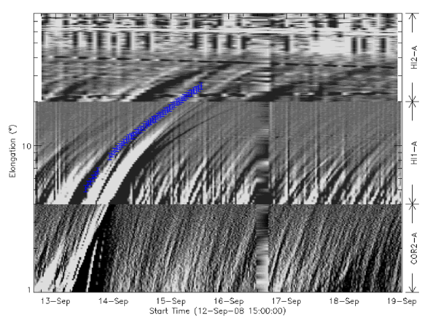
Figure 8: J-map of ecliptic plane generated from COR2, HI1 and HI2 imaging data from STA. Blue diamonds with error bars indicate the track of the CME’s leading edge viewed by STA.

Figure 9: J-map from STB.

Knowing the positions of STA and STB and the elongation angles of the CME’s leading edge measured from the two vantage points, we are able to derive the heliocentric distance and propagation direction of the CME with some assumptions. Here two widely-used triangulation methods are employed. One is the simplest triangulation, in which it is assumed that the tracks in the two J-maps describe the trajectory of the same plasma element [Liu et al., 2010]. The other one is called harmonic-mean (HM) triangulation, and it assumes that the CME is a sphere tangent to the solar surface, and the tracks in both J-maps are on the circular front but are not the same part of the CME [Lugaz et al., 2009].

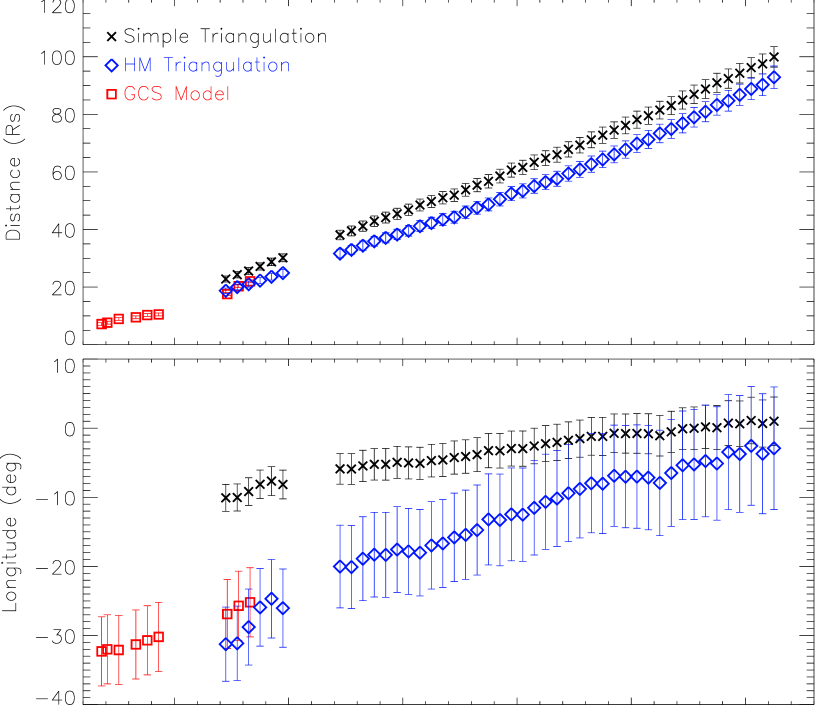
Figure 10: De-projected position of the CME’s leading edge derived by triangulation methods based on the J-maps, showing the entire propagation process of the CME from the corona to interplanetary space. For completeness, the GCS model results are also plotted.

Figure 10 shows the results from the two triangulation methods, The GCS model results are also plotted for comparison. Both triangulations show an evident westward deflected propagation of the CME in interplanetary space even if the uncertainties are taken into account. The heliocentric distances derived by HM triangulation are almost the same as those by GCS model for the last three measurements in COR2 FOV, corresponding to the period September 13 12:00 – 15:00 UT. The distances derived by the simple triangulation is systematically larger by $5-10R_{S}$. The longitude of the propagation direction derived by HM triangulation is about $-31^{\circ}$ at around 12:00 UT, and quickly increased to about $-25^{\circ}$ before the CME escaped from the FOV of COR2. The values are close to those given by GCS model. But the simple triangulation suggests that the longitude of the CME direction is about $-10^{\circ}$ in the FOV of COR2. If this is true, the CME should look more likely halo in the view from SOHO than in the view from STB, which is inconsistent with the imaging data presented in Sec.2.2. Thus for this case, HM triangulation gives more reasonable results. According to the assumptions of the simple triangulation method, it is expected to be applicable for CMEs with small extent in longitude. The longitudinal extent of the CME of interest is about $60^{\circ}$ (see Sec.3.1), which is probably too large to make the recorded tracks in both J-maps being the same part of the CME.

With the aid of the HM triangulation, it is suggested that the CME is continuously deflected in interplanetary space. The propagation longitude changed from $-25^{\circ}$ at around 15:00 UT to about $-3^{\circ}$ at 12:30 UT on September 15 when the CME’s leading edge reached about $93R_{S}$. In other words, the CME was deflected toward the west by about $22^{\circ}$ in $\sim 46$ hours or in $71R_{S}$. Obviously, the amount of the deflected angle in interplanetary space is much larger than that in the corona, suggesting that interplanetary space is a major region where the CME deflection takes place.

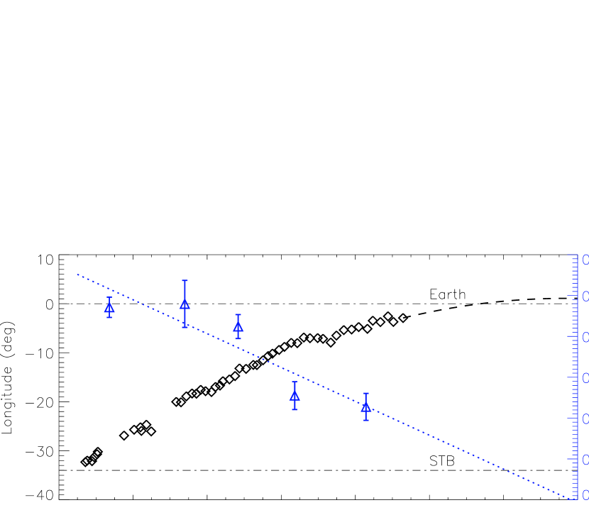
Figure 11: Longitude of the CME’s leading edge as a function of heliocentric distance is shown as diamonds. The deflection rate, i.e., deflection angle per unit distance, which is calculated on every 10 data points and scaled by the vertical axis on the right, is indicated by blue triangles. The blue dotted line is the linear fitting to the deflection rate, and dashed line shows the expected longitudes derived based on the dotted line.

The deflection rate gradually decreased from the corona to interplanetary space. Figure 11 show the longitude of the propagation direction as a function of the heliocentric distance as well as the deflection rate. Here, before 15:00 UT on September 13, we choose the data points from GCS model, and after then, we choose the data points from HM triangulation. Meanwhile, we divide all the data points into 5 groups, in each of which there are at least 10 data points, to calculate the deflection rate. The error of the deflection rate is derived from the linear fitting to the data points in each group (indicated by the error bars in Fig.11). It is found that the deflection rate is close to $0.5^{\circ}/R_{S}$ before the CME arrived at $40R_{S}$, and then gradually dropped below $0.3^{\circ}/R_{S}$. Obeying this trend, the deflection rate will approach zero sooner or later. Simply, we use a linear fitting to extrapolate the deflection rate and the resultant propagation longitude, as indicated by the lines in Figure 11. The deflection will probably cease at around $140R_{S}$, where the longitude of the CME’s propagation direction is about $1^{\circ}$. A similar deflection in the interplanetary space could be found in the paper by Lugaz et al. [2010].

These results are highly consistent with the observations. Recall that the positions of STA and STB in the ecliptic plane are $+39^{\circ}$ and $-34^{\circ}$ away from the Earth, respectively. The CME initially propagated along the longitude of about $-32^{\circ}$, and was finally deflected to about $1^{\circ}$, which made the CME being $38^{\circ}$ away from STA and $35^{\circ}$ from STB. Thus it is possible that STB observed the CME but STA did not.

4 Conclusions

In summary, by combining the data from multiple points, i.e., STA, STB, SOHO and Wind spacecraft, we studied in details the propagation process of the 2008 September 12 CME from the corona to 1 AU. The analysis definitely reveals that the CME experienced a westward deflection throughout the heliosphere. The deflection angle reaches as large as about $30^{\circ}$, among which a $20^{\circ}$-deflection occurred in interplanetary space. During the period of interest, there was no other ejection with a similar direction before or after the CME, suggesting that a CME could be significantly deflected by solar wind and interplanetary magnetic field.

Deflection not only affects which target will be hit, but also when a target will be hit. For the CME of interest, we may further approximate its front in the ecliptic plane to be a circle. As derived in Sec.3.2 that the propagation longitude of the CME at 1 AU almost coincides with the Sun-Earth line, and the CME flank glanced over STB, we may have the configuration of the CME and spacecraft as shown in Figure 12. When the CME’s flank arrives at STB, the Earth already dipped in the CME. The time difference between the arrivals of STB and the Earth is from the length difference, $\Delta l$, between $\overline{SE^{\prime}}$ and $\overline{SB}$. The angle $\alpha$ between the two lines is about $35^{\circ}$, and thus $\Delta l$ is about 0.9 AU. Considering the propagation speed of the CME observed by Wind is about 415 km s^-1, the time delay will be as large as 3.7 days. Such delays were discussed in Möstl and Davies [2013]. Actually, the CME cross-section may not be a circle but a ellipse or in a ‘pancake’ shape [e.g., Riley and Crooker, 2004; Owens et al., 2006], and the time delay will be smaller than that derived based on a circle assumption. Generally, the time delay derived above is consistent with the in-situ observations, which suggest a 2-day delay.

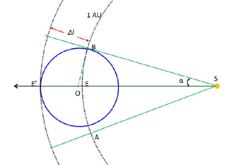
Figure 12: A diagram illustrates the time delay of CME arrival due to its circular-like front.

Thus, in the prediction of CME arrival time, the deflection combined with the CME geometry are important factors that need to be taken into account. Besides, as a consequence, the curved trajectory, along which a deflected CME actually propagates, is a minor factor influencing the accuracy of a prediction. Obviously, the length of a curved trajectory must be longer than a straight trajectory. Figure 13 shows the length difference between the curved trajectory and the heliocentric distance of this event. The length difference, what we call extra-distance here, is about $4R_{S}$. The average transit time of the CME is about 100 hours, corresponding to an average transit speed of about 400 km s^-1. If the $4R_{S}$ extra-distance was not taken into account, the prediction of the CME arrival time based on some simple empirical model will have a two-hour error, which is less than but on the same order of the typical error for CME arrival time prediction.

Figure 13: Extra-distance the CME propagating through due to its curved trajectory. It is derived based on the deflection angle shown in Fig.11.

From the above analysis, some outstanding questions about space weather forecasting emerge. What is the cause of the CME deflection and how to precisely predict the trajectory of a CME? In the following section, we will discuss the mechanism of CME deflection in interplanetary space.

5 Discussion on the mechanism of the CME deflection

It is well accepted that the deflection of a CME in the corona, usually within $5-10R_{S}$, is controlled by gradient of magnetic energy density [Shen et al., 2011a; Gui et al., 2011; Kahler et al., 2012; Zuccarello et al., 2012; Kay et al., 2013]. Generally, the magnetic energy density reaches the minimum at heliospheric current sheet, which locates near ecliptic plane during solar minima. That is why CMEs in solar minima tend to propagate toward the ecliptic plane [Cremades and Bothmer, 2004; Wang et al., 2011]. Is it also the cause of the CME deflection in interplanetary space? To answer the question, we investigate the magnetic field and current sheet at 1 AU.

The magnetic field in interplanetary space is obtained by utilizing a 3-dimensional MHD numerical method, in which a corona-interplanetary total variation diminishing (COIN-TVD) scheme is adopted [Feng et al., 2003, 2005]. Starting from Parker’s solar wind solution and the potential magnetic field extrapolated from magnetic field distribution at photosphere observed by WSO during the Carrington rotation 2074 covering the period of the CME, we use this scheme to establish a steady state of background solar wind and interplanetary magnetic field. A detailed description of the scheme and its application can be found in our previous work [Shen et al., 2007, 2009, 2011b, 2013].

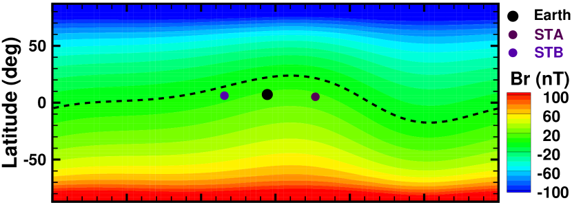
Figure 14: Carrington maps of radial component of magnetic field at $20R_{S}$ (upper panel) and 1 AU (lower panel), respectively, which are constructed by a 3-dimensional MHD simulation. Dashed lines indicate the location of heliocentric current sheet. The dots on the two maps show the positions of STA, STB and the Earth at 13:30 UT on September 13 and 04:40 UT on September 17, when the CME arrived at $20R_{S}$ and $1AU$, respectively.

Figure 14 shows the distribution of radial-component of magnetic field at $20R_{S}$ and 1 AU. The location of current sheet is indicated by the dashed lines. The positions of STA, STB and the Earth projected on the maps are marked as dots. Note that the CME arrived at $20R_{S}$ and 1 AU around 13:00 UT on September 13 and 04:30 UT on September 17, respectively. Thus the Carrington longitudes of these positions are different between the two maps. It is clear that the CME should deflect toward the north rather than the west if it still obeyed the deflection law in the corona. This opposite result suggests that there should be other causes of the deflection in interplanetary space.

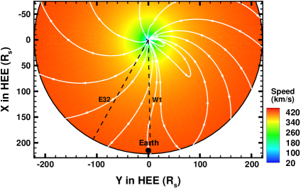
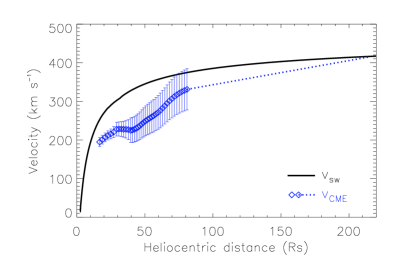
Figure 15: Left panel shows the solar wind velocity distribution in the ecliptic plane derived by 3-dimensional MHD simulation, and the right panel gives the average velocity of the solar wind within longitude of $-32^{\circ}$ and $1^{\circ}$ versus the heliocentric distance. As comparison, the CME speed is plotted as the blue diamonds and dashed line (see main text for details). The white lines in the left panel are the magnetic field lines.

In the corona, magnetic field is dominant as solar wind has not fully developed. Thus the magnetic energy density gradient guides the trajectory of a CME in the corona. However, in interplanetary space, magnetic field drops quickly and solar wind becomes dominant. Thus interaction between the CME and background solar wind should be the cause of the CME deflection in interplanetary space. A decade ago, Wang et al. [2004] proposed a kinematic model to describe the CME’s trajectory modulated by the interplanetary magnetic field carried by solar wind. In that model, the magnetic field is simply supposed to be strong enough to ensure that a CME follows the Parker spiral. It predicts that a slow CME will be deflected toward the west due to faster solar wind accumulating behind the CME and overtaking it from the east, while a fast CME will be deflected toward the east due to slower solar wind being piled up ahead of the CME and overtaken from the west [ref. to Fig.4 in Wang et al., 2004]. The model is so far the only theoretical model (except those MHD numerical simulation models) to describe the deflection of CMEs in the ecliptic plane. It is interesting to see how well the model could reproduce the trajectory of the isolated CME launched on 2008 September 12.

The physical picture of the model is similar to the solar wind deflection within a CIR, that the preceding slow solar wind has a deflection toward the west and the following fast solar wind toward the east [e.g., Siscoe et al., 1969; Gosling and Pizzo, 1999; Broiles et al., 2012]. An apparent difference between them is that the deflection speed of the solar wind within CIRs is still significant at 1 AU [Broiles et al., 2012], but that of the CME is not (Fig.11). This is because the CME speed approaches the solar wind speed at 1 AU. Thus we think that the velocity difference between two interacting system is the essential cause of the two phenomena.

The basic formula to describe the deflection of a CME is the second equation in Eq.5 of Wang et al. [2004]. Only the radial components of the CME velocity and background solar wind velocity, namely $v_{r}$ and $v_{sw}$, are required. It should be noted that the equation was developed for constant CME speed and constant solar wind speed. To accept varied speeds, we just need to slightly change the equation to the following one

$$d\phi=\Omega\left(\frac{1}{v_{r}}-\frac{1}{v_{sw}}\right)dr$$ (1)

in which $\phi$ is the longitude, $r$ the heliocentric distance and $\Omega$ the angular speed of the Sun’s rotation. For completeness, a derivation of the above equation, different but much briefer than that in Wang et al. [2004], is given in the Appendix. The total change of longitude of a CME is the integral of Eq.1, which could be numerically calculated once we know $v_{sw}$ and $v_{r}$, which are both functions of heliocentric distance $r$.

To obtain the solar wind speed, $v_{sw}$, we utilize the MHD numerical method again. The left panel of Figure 15 shows the radial component of the solar wind velocity in ecliptic plane with interplanetary magnetic field lines superimposed. Since the previous analysis have suggested that the CME was deflected from $-32^{\circ}$ to $1^{\circ}$, we use the averaged solar wind speed between the two longitudes. The profile of the speed is shown in the right panel of Figure 15. Within first $20R_{S}$ the background solar wind quickly accelerates to 300 km s^-1, and then gradually accelerates to more than 410 km s^-1 at 1 AU.

For comparison, the CME bulk propagation speed, $v_{r}$, is plotted as blue diamonds and a dashed line in the right panel of Figure 15. The speed below $90R_{S}$ is derived from the height time plot of the CME leading edge in Figure 10 with expansion speed deducted. Here we assume that the CME expanded with a constant angular width. At 1 AU, Wind data suggests that the CME expansion speed is about 45 km s^-1, the bulk propagation speed is about 415 km s^-1 and the radius is about 0.14 AU. It means that the bulk propagation speed of the CME is 11% smaller than the speed of the CME leading edge, and the heliocentric distance is 14% shorter than that of the leading edge. The speed beyond $90R_{S}$ is simply obtained by a linear extrapolation.

By inputting $v_{sw}$ and $v_{r}$ into our model, we find that the propagation longitude of the CME changes about $8^{\circ}$ from the initial value of $-29^{\circ}$ to $-21^{\circ}$, as shown by the solid line in Figure 16. The amount of the deflection predicted by the model is much smaller than that derived from observations. Considering that deflection in our model is substantially due to the difference between $v_{r}$ and $v_{sw}$, we could expect that the error in either velocity will cause the error in deflection angle. The two dashed lines show the different CME trajectory if the CME velocity was 15% higher (the lower line, suggesting a smaller deflection) or lower (the upper line, suggesting a larger deflection). The latter suggests a $20^{\circ}$ deflection, closer to but still smaller than the observations.

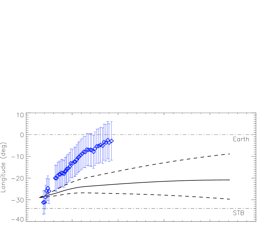
Figure 16: Observed (blue diamonds with error bars) and model predicted (black lines) longitudes of the CME. The two dashed lines indicate the predicted longitudes by considering $\pm 15\%$ error in the CME velocity. Refer to Sec.5 for details.

In summary, the deflection of a CME in interplanetary space has a different cause of that in the corona. Although our kinematic model predicts a westward deflection of the CME originating on September 12, the modeled trajectory is not good enough. The deviation between the model predicted and the observed trajectory could be from the highly-ideal assumptions used in our model and/or other unknown factors/processes that take place during the solar wind-CME interaction. For example, we only consider the Parker spiral magnetic field lines shaped by solar wind but do not fully take the kinetic energy carried by the solar wind into account. But in interplanetary space, the kinetic energy should be stronger than magnetic energy.

Appendix A Derivation of kinematic model of the CME deflection

The model assumes that the background solar wind and interplanetary magnetic field (IMF) is dominant and the CME is a fluid parcel, so that the CME in the ecliptic plane tends to move following IMF lines. Figure 17 illustrates the model. Dotted lines are Parker spiral magnetic field lines, and the solid line is the unaffected field line connecting to the CME which moves radially with a speed slower than the background solar wind. Since magnetic field lines cannot cross over each other, the slow CME should be deflected toward the west to make the solid line coinciding with the spiral magnetic field line starting from the same place on the Sun (or the IMF lines will be deformed if CME kinetic energy was dominant). Thus the model is more suitable for slow CMEs.

Figure 17: Illustration of the model.

The detailed derivation of the model was given in [Wang et al., 2004]. Here, we present another approach to derive the model. It is a 2-D model in the ecliptic plane. Let $v_{sw}$ be the solar wind speed, $\Omega$ the solar rotation, $\varphi_{i}$ the initial longitude and $t$ the time since the plasma element left the Sun, then the Parker spiral IMF shown in Figure 17 is given by

$$r_{0} = v_{sw}t$$ (2)

$$\varphi_{0} = \varphi_{i}-\Omega t$$ (3)

Assuming that the CME is a plasma parcel with a radial speed of $v_{r}$, the magnetic field line drawn by the CME is given by

$$r = v_{r}t$$ (4)

$$\varphi = \varphi_{i}-\Omega t+\Delta\phi(t)$$ (5)

which should satisfy the following condition because the CME is assumed to follow the Parker spiral of the IMF,

$$\frac{r_{0}}{\varphi_{0}-\varphi_{i}}=\frac{r}{\varphi-\varphi_{i}}$$ (6)

Here $\Delta\phi$ is the time-dependent or distance-dependent deflection angle of the CME. It is easy to derive that

$$\Delta\phi(t)=\frac{v_{sw}-v_{r}}{v_{sw}}\Omega t$$ (7)

or

$$\Delta\phi(r) = \frac{v_{sw}-v_{r}}{v_{sw}v_{r}}\Omega r$$ (8)

$$= \left(\frac{1}{a}-\frac{1}{a_{0}}\right)r$$

in which $a=v_{r}/\Omega$ and $a_{0}=v_{sw}/\Omega$. Eq.8 is exactly the same as Eq.5 in Wang et al. [2004].

The above derivation uses the constant velocity for both solar wind and the CME. To accept varied velocity, we just convert Eq.2–5 to the differential form

$$\left\{\begin{array}[]{l}dr_{0}=v_{sw}dt\\ d\varphi_{0}=-\Omega dt\end{array}\right.$$ (11)

$$\left\{\begin{array}[]{l}dr=v_{r}dt\\ d\varphi=-\Omega dt+d\phi(t)\end{array}\right.$$ (14)

Then we can get the deflection angle

$$d\phi = \frac{v_{sw}-v_{r}}{v_{sw}}\Omega dt$$ (15)

$$= \left(\frac{1}{v_{r}}-\frac{1}{v_{sw}}\right)\Omega dr$$

as well as the angular velocity of the CME

$$\omega=\frac{d\phi}{dt}=\frac{v_{sw}-v_{r}}{v_{sw}}\Omega$$ (16)

The interaction between solar wind and CMEs will not only affect the angular motion but also the radial motion, i.e., acceleration/deceleration, of the CME. The model can only predict the change of angular motion. The change of the radial motion caused by the solar wind interaction has been taken into account by adopting changing $v_{r}$ of the CME as derived from the heliospheric observations.

References

- Acuña et al. [2008] Acuña, M. H., D. Curtis, J. L. Scheifele, C. T. Russell, P. Schroeder, A. Szabo, and J. G. Luhmann, The STEREO/IMPACT magnetic field experiment, Space Sci. Rev., 136, 203–226, 2008.
- Berdichevsky et al. [2002] Berdichevsky, D., C. Farrugia, B. Thompson, R. Lepping, D. Reames, M. Kaiser, J. Steinberg, S. Plunkett, and D. Michels, Halo-coronal mass ejections near the 23rd solar minimum: lift-off, inner heliosphere, and in situ (1 AU) signatures, Ann. Geophys., 20, 891, 2002.
- Broiles et al. [2012] Broiles, T. W., M. I. Desai, and D. J. McComas, Formation, shape, and evolution of magnetic structures in CIRs at 1 AU, J. Geophys. Res., 117, A03,102, 2012.
- Brueckner et al. [1995] Brueckner, G. E., R. A. Howard, M. J. Koomen, C. M. Korendyke, D. J. Michels, J. D. Moses, D. G. Socker, K. P. Dere, P. L. Lamy, A. Llebaria, M. V. Bout, R. Schwenn, G. M. Simnett, D. K. Bedford, and C. J. Eyles, The large angle spectroscopic coronagraph (LASCO), Sol. Phys., 162, 357–402, 1995.
- Burlaga et al. [1981] Burlaga, L., E. Sittler, F. Mariani, and R. Schwenn, Magnetic loop behind an interplanetary shock: Voyager, Helios, and IMP 8 observations, J. Geophys. Res., 86, 6673–6684, 1981.
- Cane and Richardson [2003] Cane, H. V., and I. G. Richardson, Interplanetary coronal mass ejections in the near-earth solar wind during 1996–2002, J. Geophys. Res., 108(A4), 1156, doi:10.1029/2002JA009,817, 2003.
- Cane et al. [1998] Cane, H. V., I. G. Richardson, and O. C. St Cyr, The interplanetary events of January-May, 1997 as inferred from energetic particle data, and their relationship with solar events, Geophys. Res. Lett., 25, 2517–2520, 1998.
- Cane et al. [2000] Cane, H. V., I. G. Richardson, and O. C. St. Cyr, Coronal mass ejections, interplanetary ejecta and geomagnetic storms, Geophys. Res. Lett., 27, 3591–3594, 2000.
- Cid et al. [2012] Cid, C., H. Cremades, A. Aran, C. Mandrini, B. Sanahuja, B. Schmieder, M. Menvielle, L. Rodriguez, E. Saiz, Y. Cerrato, S. Dasso, C. Jacobs, C. Lathuillere, and A. Zhukov, Can a halo cme from the limb be geoeffective?, J. Geophys. Res., 117, A11,102, 2012.
- Cremades and Bothmer [2004] Cremades, H., and V. Bothmer, On the three-dimensional configuration of coronal mass ejections, Astron. & Astrophys., 422, 307–322, 2004.
- Cremades et al. [2006] Cremades, H., V. Bothmer, and D. Tripathi, Properties of structured coronal mass ejections in solar cycle 23, Adv. in Space Res., 38, 461–465, 2006.
- Davies et al. [2009] Davies, J. A., R. A. Harrison, A. P. Rouillard, N. R. Sheeley, C. H. Perry, D. Bewsher, C. J. Davis, C. J. Eyles, S. R. Crothers, and D. S. Brown, A synoptic view of solar transient evolution in the inner heliosphere using the heliospheric imagers on STEREO, Geophys. Res. Lett., 36, L02,102, 2009.
- DeForest et al. [2013] DeForest, C. E., T. A. Howard, and D. J. McComas, Tracking coornal features from the low corona to earth: A quantitative analysis of the 2008 december 12 coronal mass ejection, Astrophys. J., 769, 43(13pp), 2013.
- Farrugia et al. [1993] Farrugia, C. J., L. F. Burlaga, V. A. Osherovich, I. G. Richardson, M. P. Freeman, R. P. Lepping, and A. J. Lazarus, A study of an expanding interplanetary magnetic cloud and its interaction with the earth’s magnetosphere – the interplanetary aspect, J. Geophys. Res., 98(A5), 7621–7632, 1993.
- Feng et al. [2003] Feng, X., S. T. Wu, F. Wei, and Q. Fan, A class of TVD type combined numerical scheme for MHD equations with a survey about numerical methods in solar wind simulations, Space Sci. Rev., 107, 43–53, 2003.
- Feng et al. [2005] Feng, X., C. Xiang, D. Zhong, and Q. Fan, A comparative study on 3-d solar wind structure observed by Ulysses and MHD simulation, Chinese Sci. Bull., 50, 672–678, 2005.
- Galvin et al. [2008] Galvin, A. B., L. M. Kistler, M. A. Popecki, C. J. Farrugia, K. D. C. Simunac, L. Ellis, E. Mobius, M. A. Lee, M. Boehm, J. Carroll, A. Crawshaw, M. Conti, P. Demaine, S. Ellis, J. A. Gaidos, J. Googins, M. Granoff, A. Gustafson, D. Heirtzler, B. King, U. Knauss, J. Levasseur, S. Longworth, K. Singer, S. Turco, P. Vachon, M. Vosbury, M. Widholm, L. M. Blush, R. Karrer, P. Bochsler, H. Daoudi, A. Etter, J. Fischer, J. Jost, A. Opitz, M. Sigrist, P. Wurz, B. Klecker, M. Ertl, E. Seidenschwang, R. F. Wimmer-Schweingruber, M. Koeten, B. Thompson, and D. Steinfeld, The plasma and suprathermal ion composition (PLASTIC) investigation on the STEREO observatories, Space Sci. Rev., 136, 437–486, 2008.
- Gopalswamy et al. [2003] Gopalswamy, N., M. Shimojo, W. Lu, S. Yashiro, K. Shibasaki, and R. A. Howard, Prominence eruptions and coronal mass ejection: A statistical study using microwave observations, Astrophys. J., 586, 562–578, 2003.
- Gopalswamy et al. [2004] Gopalswamy, N., S. Yashiro, S. Krucker, G. Stenborg, and R. A. Howard, Intensity variation of large solar energetic particle events associated with coronal mass ejections, J. Geophys. Res., 109, A12,105, 2004.
- Gopalswamy et al. [2009] Gopalswamy, N., P. Mäkelä, H. Xie, S. Akiyama, and S. Yashiro, CME interactions with coronal holes and their interplanetary consequences, J. Geophys. Res., 114, A00A22, 2009.
- Gosling and Pizzo [1999] Gosling, J. T., and V. J. Pizzo, Formation and evolution of corotating interaction regions and their three dimensional structure, Space Sci. Rev., 89, 21–52, 1999.
- Gosling et al. [1987] Gosling, J. T., D. N. Baker, S. J. Bame, W. C. Feldman, R. D. Zwickl, and E. J. Smith, Bidirectional solar wind electron heat flux events, J. Geophys. Res., 92, 8519–8535, 1987.
- Gui et al. [2011] Gui, B., C. Shen, Y. Wang, P. Ye, J. Liu, S. Wang, and X. Zhao, Quantitative analysis of cme deflections in the corona, Sol. Phys., 271, 111–139, 2011.
- Howard et al. [2008] Howard, R. A., J. Moses, A. Vourlidas, and et al., Sun earth connection coronal and heliospheric investigation (SECCHI), Space Sci. Rev., 136, 67–115, 2008.
- Isavnin et al. [2013] Isavnin, A., A. Vourlidas, and E. Kilpua, Three-dimensional evolution of erupted flux ropes from the Sun (2–20 r) to 1 AU, Sol. Phys., 284, 203–215, 2013.
- Kahler et al. [2012] Kahler, S. W., S. Akiyama, and N. Gopalswamy, Deflections of fast coronal mass ejections and the properties of associated solar energetic particle events, Astrophys. J., 754, 100(7pp), 2012.
- Kaiser et al. [2008] Kaiser, M. L., T. A. Kucera, J. M. Davila, O. C. St. Cyr, M. Guhathakurta, and E. Christian, The stereo mission: An introduction, Space Sci. Rev., 136, 5–16, 2008.
- Kay et al. [2013] Kay, C., M. Opher, and R. M. Evans, Forecasting a coronal mass ejection’s altered trajectory: ForeCAT, Astrophys. J., 775, 5(17pp), 2013.
- Kilpua et al. [2009] Kilpua, E. K. J., J. Pomoell, A. Vourlidas, R. Vainio, J. Luhmann, Y. Li, P. Schroeder, A. B. Galvin, and K. Simunac, STEREO observations of interplanetary coronal mass ejections and prominence deflection during solar minimum period, Ann. Geophys., 27, 4491–4503, 2009.
- Lepping et al. [1990] Lepping, R. P., J. A. Jones, and L. F. Burlaga, Magnetic field structure of interplanetary magnetic clouds at 1 AU, J. Geophys. Res., 95, 11,957–11,965, 1990.
- Lepping et al. [1995] Lepping, R. P., M. H. Acuña, L. F. Burlaga, W. M. Farrell, J. A. Slavin, K. H. Schatten, F. Mariani, N. F. Ness, F. M. Neubauer, Y. C. Whang, J. B. Byrnes, R. S. Kennon, P. V. Panetta, J. Scheifele, and E. M. Worley, The Wind magnetic field investigation, Space Sci. Rev., 71, 207–229, 1995.
- Lin et al. [1995] Lin, R. P., K. A. Anderson, S. Ashford, C. Carlson, D. Curtis, R. Ergun, D. Larson, J. McFadden, M. McCarthy, G. K. Parks, H. Rème, J. M. Bosqued, J. Coutelier, F. Cotin, C. D’Uston, K.-P. Wenzel, T. R. Sanderson, J. Henrion, J. C. Ronnet, and G. Paschmann, A three-dimensional plasma and energetic particle investigation for the Wind spacecraft, Space Sci. Rev., 71, 125–153, 1995.
- Lindsay et al. [1999] Lindsay, G. M., J. G. Luhmann, C. T. Russell, and J. T. Gosling, Relationships between coronal mass ejection speeds from coronagraph images and interplanetary characteristics of associated interplanetary coronal mass ejections, J. Geophys. Res., 104, 12,515, 1999.
- Liu et al. [2010] Liu, Y., J. A. Davies, J. G. Luhmann, A. Vourlidas, S. D. Bale, and R. P. Lin, Geometric triangulation of imaging observations to track coronal mass ejections continuously out to 1 AU, Astrophys. J., 710, L82–L87, 2010.
- Lopez and Freeman [1986] Lopez, R. E., and J. W. Freeman, Solar wind proton temperature-velocity relationship, J. Geophys. Res., 91, 1701, 1986.
- Lugaz [2010] Lugaz, N., Accuracy and limitations of fitting and stereoscopic methods to determine the direction of coronal mass ejections from heliospheric imagers observations, Sol. Phys., 267, 411–429, 2010.
- Lugaz et al. [2009] Lugaz, N., A. Vourlidas, and I. I. Roussev, Deriving the radial distances of wide coronal mass ejections from elongation measurements in the heliosphere application to CME-CME interaction, Ann. Geophys., 27, 3479–3488, 2009.
- Lugaz et al. [2010] Lugaz, N., J. N. Hernandez-Charpak, I. I. Roussev, C. J. Davis, A. Vourlidas, and J. A. Davies, Determining the azimuthal properties of coronal mass ejections from multi-spacecraft remote-sensing observations with STEREO SECCHI, Astrophys. J., 715, 493–499, 2010.
- Lugaz et al. [2011] Lugaz, N., C. Downs, K. Shibata, I. I. Roussev, A. Asai, and T. I. Gombosi, Numerical investigation of a coronal mass ejection from an anemone active region: Reconnection and defelction of the 2005 August 22 eruption, Astrophys. J., 738, 127(13pp), 2011.
- Lugaz et al. [2012] Lugaz, N., C. J. Farrugia, J. A. Davies, C. Mostl, C. J. Davis, I. I. Roussev, and M. Temmer, The deflection of the two interacting coronal mass ejections of 2010 may 23-24 as revealed by combined in site measurements and heliospheric imaging, Astrophys. J., 759, 68(13pp), 2012.
- Ma et al. [2010] Ma, S., G. D. R. Attrill, L. Golub, and J. Lin, Statistical study of coronal mass ejections with and without distinct low coronal signatures, Astrophys. J., 722, 289–301, 2010.
- MacQueen et al. [1986] MacQueen, R. M., A. J. Hundhausen, and C. W. Conover, The propagation of coronal mass ejection transients, J. Geophys. Res., 91, 31–38, 1986.
- Möstl and Davies [2013] Möstl, C., and J. A. Davies, Speeds and arrival times of solar transients approximated by self-similar expanding circular fronts, Sol. Phys., 285, 411–423, 2013.
- Ogilvie et al. [1995] Ogilvie, K. W., D. J. Chornay, R. J. Fritzenreiter, F. Hunsaker, J. Keller, J. Lobell, G. Miller, J. D. Scudder, J. Sittler, E. C., R. B. Torbert, D. Bodet, G. Needell, A. J. Lazarus, J. T. Steinberg, J. H. Tappan, A. Mavretic, and E. Gergin, SWE, a comprehensive plasma instrument for the Wind spacecraft, Space Sci. Rev., 71, 55–77, 1995.
- Owens et al. [2006] Owens, M. J., V. G. Merkin, and P. Riley, A kinematically distorted flux rope model for magnetic clouds, J. Geophys. Res., 111, A03,104, 2006.
- Plunkett et al. [2001] Plunkett, S. P., B. J. Thompson, O. C. St. Cyr, and R. A. Howard, Solar source regions of coronal mass ejections and their geomagnetic effects, J. Atmos. Solar-Terres. Phys., 63, 389–402, 2001.
- Richardson and Cane [1995] Richardson, I. G., and H. V. Cane, Regions of abnormally low proton temperature in the solar wind (1965–1991) and their association with ejecta, J. Geophys. Res., 100(A12), 23,397–23,412, 1995.
- Riley and Crooker [2004] Riley, P., and N. U. Crooker, Kinematic treatment of coronal mass ejection evolution in the solar wind, Astrophys. J., 600, 1035–1042, 2004.
- Robbrecht et al. [2009] Robbrecht, E., S. Patsourakos, and A. Vourlidas, No trace left behind: STEREO observation of a coronal mass ejection without low coronal signatures, Astrophys. J., 701, 283–291, 2009.
- Rodriguez et al. [2011] Rodriguez, L., M. Mierla, A. Zhukov, M. West, and E. Kilpua, Linking remote-sensing and in situ observations of coronal mass ejections using STEREO, Sol. Phys., 270, 561–573, 2011.
- Schwenn et al. [2005] Schwenn, R., A. Dal Lago, E. Huttunen, and W. D. Gonzalez, The association of coronal mass ejections with their effects near the Earth, Ann. Geophys., 23(3), 1033–1059, 2005.
- Shen et al. [2011a] Shen, C., Y. Wang, B. Gui, P. Ye, and S. Wang, Kinematic evolution of a slow CME in near solar space viewed by STEREO-B in October 8, 2007, Sol. Phys., 269, 389–400, 2011a.
- Shen et al. [2012] Shen, C., Y. Wang, S. Wang, Y. Liu, R. Liu, A. Vourlidas, B. Miao, P. Ye, J. Liu, and Z. Zhou, Super-elastic collision of large-scale magnetized plasmoids in the heliosphere, Nature Phys., 8, 923–928, 2012.
- Shen et al. [2007] Shen, F., X. Feng, S. T. Wu, and C. Xiang, Three-dimensional MHD simulation of CMEs in three-dimensional background solar wind with the self-consistent structure on the source surface as input: Numerical simulation of the January 1997 Sun-Earth connection event, J. Geophys. Res., 112, A06,109, 2007.
- Shen et al. [2009] Shen, F., X. Feng, and W. B. Song, An asynchronous and parallel time-marching method: application to the three-dimensional MHD simulation of the solar wind, Science in china Series E: Technological Sciences, 52, 2895–2902, 2009.
- Shen et al. [2011b] Shen, F., X. S. Feng, Y. Wang, S. T. Wu, W. B. Song, J. P. Guo, and Y. F. Zhou, Three-dimensional MHD simulation of two coronal mass ejections’ propagation and interaction using a successive magnetized plasma blobs model, J. Geophys. Res., 116, A09,103, 2011b.
- Shen et al. [2013] Shen, F., C. Shen, Y. Wang, X. Feng, and C. Xiang, Could the collision of cmes in the heliosphere be super-elastic? validation through three-dimensional simulations, Geophys. Res. Lett., 40, 1457–1461, 2013.
- Siscoe et al. [1969] Siscoe, G. L., B. Goldstein, and A. J. Lazarus, An east-west asymmetry in the solar wind velocity, J. Geophys. Res., 74, 1759, 1969.
- Thernisien [2011] Thernisien, A., Implementation of the graduated cylindrical shell model for the three-dimensional reconstruction of coronal mass ejections, Astrophys. J. Suppl. Ser., 194, 33, 2011.
- Thernisien et al. [2009] Thernisien, A., A. Vourlidas, and R. Howard, Forward modeling of coronal mass ejections using STEREO/SECCHI data, Sol. Phys., 256, 111–130, 2009.
- Vourlidas et al. [2013] Vourlidas, A., B. J. Lynch, R. A. Howard, and Y. Li, How many cmes have flux ropes? deciphering the signatures of shocks, flux ropes, and prominences in coronagraph observations of cmes, Sol. Phys., 284, 179–201, 2013.
- Wang et al. [2004] Wang, Y., C. Shen, P. Ye, and S. Wang, Deflection of coronal mass ejection in the interplanetary medium, Sol. Phys., 222, 329–343, 2004.
- Wang et al. [2006] Wang, Y., X. Xue, C. Shen, P. Ye, S. Wang, and J. Zhang, Impact of the major coronal mass ejections on geo-space during September 7 – 13, 2005, Astrophys. J., 646, 625–633, 2006.
- Wang et al. [2011] Wang, Y., C. Chen, B. Gui, C. Shen, P. Ye, and S. Wang, Statistical study of coronal mass ejection source locations: Understanding cmes viewed in coronagraphs, J. Geophys. Res., 116, A04,104, doi:10.1029/2010JA016,101, 2011.
- Wang et al. [2002] Wang, Y. M., P. Z. Ye, S. Wang, G. P. Zhou, and J. X. Wang, A statistical study on the geoeffectiveness of earth-directed coronal mass ejections from March 1997 to December 2000, J. Geophys. Res., 107(A11), 1340, doi:10.1029/2002JA009,244, 2002.
- Webb et al. [1996] Webb, D., B. Jackson, and P. Hick, Geomagnetic storms and heliospheric CMEs as viewed from HELIOS, in Solar Drivers of Interplanetary and Terrestrial Disturbances, ASP Conference Series, vol. 95, p. 167, 1996.
- Webb et al. [2000] Webb, D. F., E. W. Cliver, N. U. Crooker, O. C. St. Cyr, and B. J. Thompson, Relationship of halo coronal mass ejections, magnetic clouds, and magnetic storms, J. Geophys. Res., 105(A4), 7491–7508, 2000.
- Webb et al. [2001] Webb, D. F., N. U. Crooker, S. P. Plunkett, and O. C. St. Cyr, The solar sources of geoeffective structures, in Space Weather, edited by S. Paul, J. S. Howard, and L. S. George, Geophys. Monogr. Ser. 125, pp. 123–142, AGU, 2001.
- Yang et al. [2012] Yang, J., Y. Jiang, R. Zheng, Y. Bi, J. Hong, and B. Yang, Sympathetic filament eruptions from a bipolar helmet streamer in the Sun, Astrophys. J., 745, 9, 2012.
- Yermolaev et al. [2005] Yermolaev, Y. I., M. Yermolaev, G. Zastenker, L. Zelenyi, A. Petrukovich, and J.-A. Sauvaud, Statistical studies of geomagnetic storm dependencies on solar and interplanetary events: a review, Planet. Space Sci., 53, 189–196, 2005.
- Zhang et al. [2003] Zhang, J., K. P. Dere, R. A. Howard, and V. Bothmer, Identification of solar sources of major geomagnetic storms between 1996 and 2000, Astrophys. J., 582, 520–533, 2003.
- Zhang et al. [2007] Zhang, J., I. G. Richardson, D. F. Webb, N. Gopalswamy, E. Huttunen, J. C. Kasper, N. V. Nitta, W. Poomvises, B. J. Thompson, C.-C. Wu, S. Yashiro, and A. N. Zhukov, Solar and interplanetary sources of major geomagnetic storms (Dst -100 nT) during 1996-2005, J. Geophys. Res., 112, A10,102, 2007.
- Zhou and Feng [2013] Zhou, Y., and X. S. Feng, MHD numerical study of the latitudinal deflection of coronal mass ejection, J. Geophys. Res., 118, 6007–6018, 2013.
- Zuccarello et al. [2012] Zuccarello, F. P., A. Bemporad, C. Jacobs, M. Mierla, S. Poedts, and F. Zuccarello, The role of streamers in the deflection of coronal mass ejections: Comparison between STEREO three-dimensional reconstructions and numerical simulations, Astrophys. J., 744, 66(14pp), 2012.