Entanglement of helicity and energy in kinetic Alfvén wave/whistler turbulence

Abstract

The role of magnetic helicity is investigated in kinetic Alfvén wave and oblique whistler turbulence in presence of a relatively intense external magnetic field $b_{0}{\bf e_{\parallel}}$. In this situation, turbulence is strongly anisotropic and the fluid equations describing both regimes are the reduced electron magnetohydrodynamics (REMHD) whose derivation, originally made from the gyrokinetic theory, is also obtained here from compressible Hall MHD. We use the asymptotic equations derived by Galtier & Bhattacharjee (2003) to study the REMHD dynamics in the weak turbulence regime. The analysis is focused on the magnetic helicity equation for which we obtain the exact solutions: they correspond to the entanglement relation, $n+\tilde{n}=-6$, where $n$ and $\tilde{n}$ are the power law indices of the perpendicular (to ${\bf b_{0}}$) wave number magnetic energy and helicity spectra respectively. Therefore, the spectra derived in the past from the energy equation only, namely $n=-2.5$ and $\tilde{n}=-3.5$, are not the unique solutions to this problem but rather characterize the direct energy cascade. The solution $\tilde{n}=-3$ is a limit imposed by the locality condition; it is also the constant helicity flux solution obtained heuristically. The results obtained offer a new paradigm to understand solar wind turbulence at sub-ion scales where it is often observed that $-3<n<-2.5$.

1 Introduction

Fluctuations in space plasmas exhibit a multitude of time and length scales such as the ion or electron cyclotron frequencies, inertial lengths and Larmor radii. For example, in the solar wind where in situ measurements are accessible the turbulent velocity, magnetic and density fluctuation spectra are characterized by extended power laws observed in the frequency range $10^{-5}$ Hz $\leq f\leq 10^{2}$ Hz (Matthaeus & Goldstein, 1982; Goldstein & Roberts, 1999; Galtier, 2006a; Carbone, 2012). As expected, when one probes the solar wind plasma towards high frequencies, the physical properties evolve and several breaks in the magnetic field fluctuation spectrum are detected (Smith et al., 2006; Alexandrova et al., 2009; Sahraoui et al., 2010). In figure 1 a schematic view of the magnetic field fluctuation spectrum observed in the solar wind is reported. For example, the break detected at the frequency $f_{1}\sim 0.5$ Hz is attributed to the decoupling between ions and electrons and defines, therefore, the scale at which one has to abandon the standard magnetohydrodynamic (MHD) model. The precise mechanism that drives the physics is still unclear: basically, the frequency range $f_{1}\leq f\leq f_{3}$ is seen as either a dissipative range or/and a new turbulence regime. The difficulty resides, in particular, in the collisionless nature of the plasma and also its anisotropy.

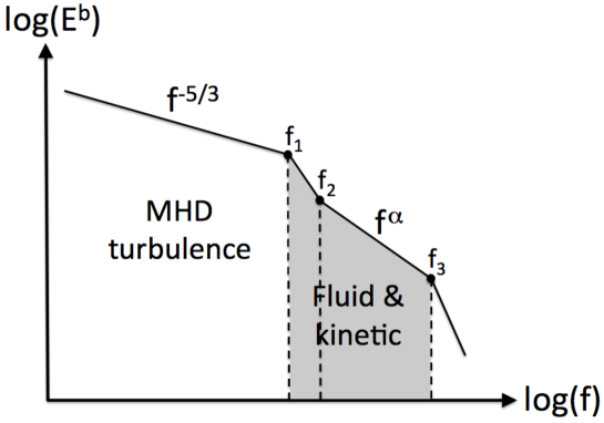
Figure 1: Schematic view of the magnetic fluctuation spectrum observed in the solar wind at one astronomical unit. Three breaks are shown at frequencies $f_{1}$, $f_{2}$ and $f_{3}$. The large scale ($f<f_{1}\sim 0.5$Hz) spectrum, characterized by a narrow range of power law indices with a peak near $-5/3$ (Smith et al., 2006), is generally interpreted as an MHD turbulence cascade. At sub-ion scales ($f>f_{1}$) the physical properties change drastically. After a stiff transition between breaks $f_{1}$ and $f_{2}$ (Sahraoui et al., 2010), a $f^{\alpha}$ spectrum is clearly observed such that $\alpha\in[-3.1,-2.5]$ with a value often around $-2.8$ (Sahraoui et al., 2013). At sub-electron scales ($f>f_{3}\sim 50$Hz) another stiff variation – possibly in power law – is measured but the instrumental noise level is quickly reached. The gray part is the frequency domain where both kinetic Alfvén waves and whistler waves are detected and where both fluid and kinetic models are used.

Note that typical solar wind plasma parameters at one astronomical unit are: $\beta_{i}\sim\beta_{e}\sim 1$ (ratio of thermal to magnetic pressure for ion $\beta_{i}$ and electron $\beta_{e}$), $T_{i}/T_{e}\sim 1$ (ratio of ion to electron temperature), $d_{i}\sim 100$ km (ion inertial length) and $f_{ci}\sim 0.1$ Hz (ion cyclotron frequency).

Both kinetic and fluid models are used to investigate the difficult problem of plasma turbulence at sub-ion scales (Ghosh & Goldstein, 1997; Schekochihin et al., 2009; Meyrand & Galtier, 2010; Rudakov et al., 2011). For example, for the solar wind we often evoke kinetic Alfvén waves (KAW) and whistler waves (Sahraoui et al., 2012) which can be both excited for scales smaller than $d_{i}$. The main difference between KAW and whistlers is in the dynamics of ions which rapidly adjust to the fluctuating electric potential in the former case, whereas they are dynamically irrelevant in the latter. By definition, classical fluid models (e.g. Hall MHD or electron MHD) are not able to catch kinetic effects and their use at sub-ion scales is mainly relevant for the investigation of the turbulent dynamics. In the solar wind case it is believed that the origin of the power law spectra for $f>f_{2}$ (see figure 1) could be attributed mainly to turbulence which would imply that kinetic effects are irrelevant to understand the statistical properties of the magnetic fluctuations (Matthaeus et al., 2014). Following this remark, we shall recall below the limit of validity of the fluid models. In the fluid case, the electron momentum equation with all electron inertia terms neglected gives the generalized ideal Ohm’s law (in SI units):

$${\bf E}+{\bf u}_{e}\times{\bf b}-{\nabla p_{e}\over n_{e}e}=0\,,$$ (1)

where ${\bf E}$ is the electric field, ${\bf u}_{e}$ the electron velocity, ${\bf b}$ the magnetic field, $n_{e}$ the electron density, $e$ the magnitude of the electron charge, and $p_{e}$ the electron pressure. The introduction of equation (1) into the Maxwell–Faraday’s law, with the MHD momentum equation, and for example the polytropic closure, lead to the so-called Hall MHD system in which the Hall effect becomes dominant at length scales smaller than the ion inertial length $d_{i}$ ($d_{i}\equiv c/\omega_{pi}$ with $c$ the speed of light and $\omega_{pi}$ the ion plasma frequency) and time-scales of the order, or shorter than, the ion cyclotron period $\omega_{ci}^{-1}$. Note that in Hall MHD, the electron pressure $p_{e}$ is assumed to be a scalar (this can be justified in the collisional limit or in the isothermal electron fluid approximation (Schekochihin et al., 2009)). The limit of validity of Hall MHD may be discussed at the level of the dispersion relation. (We focus the discussion on frequencies where the electron inertia is not felt.) As shown by Hirose et al. (2004), the Hall MHD dispersion relation is a rigorous limit of Vlasov-Maxwell kinetic theory in the limit of cold ions, i.e. $T_{i}=0$. Under this limit, the ion Landau resonance becomes negligible which explains why physically the fluid model may be relevant. However, two important comments have to made here. First, this limitation was discussed quantitatively by Howes (2006) (see also Sahraoui et al. (2012)) from the numerical resolution of the dispersion relations. It was found that even at $T_{i}=T_{e}$ (with $\beta=1$) the parallel whistler, oblique whistler and kinetic Alfvén waves are well described by Hall MHD whereas for example the slow mode represents an unphysical/spurious wave that does not exist in a weakly collisional plasma. Second, the simple analytical demonstration made on the dispersion relation does not say anything about the validity of Hall MHD in the full turbulent regime for which the statistical contribution of kinetic effects is still not well documented. If this contribution is negligible (Matthaeus et al., 2014) or if the three previous waves are not affected by the spurious waves, then Hall MHD may be a relevant model for plasmas even when $T_{i}\sim T_{e}$ (and $\beta\sim 1$). An example is given with incompressible ($\beta\gg 1$) Hall MHD in the regime of wave turbulence. As shown by Galtier (2006b), it is possible to get spectral predictions only for the right circularly polarized wave (so without the feedback of the left circularly polarized wave) which may describe parallel whistler, oblique whistler or KAW (see the discussion in section 2). Also, it is though that as long as a fluid model like Hall MHD is able to predict statistical properties compatible with the observations the pure turbulent cascade scenario has to be considered as a central mechanism to transfer energy scale by scale until the electron scales. Beyond the solar wind, Hall MHD is widely used to investigate several questions such as the origin of the fast magnetic reconnection (Bhattacharjee, 2004; Shepherd & Cassak, 2010) or the formation and disruption of Alfvénic filaments (Dreher et al., 2005).

Three-dimensional Hall MHD turbulence is much more difficult to investigate numerically than pure MHD because the Hall effect brings a new kind of nonlinear term with a second-order derivative which sometimes forces us to use lower-dimensional models (Ghosh et al., 1996; Galtier & Buchlin, 2007). Because of this difficulty, it is interesting to investigate first the incompressible limit for which the Hall effect is asymptotically large, i.e. the so-called electron MHD regime (Kingsep et al., 1990; Goldreich & Reisenegger, 1992; Das, 1999; Diamond et al., 2011). In this limit, the ions can be considered as a motionless neutralizing background such that the electron flow determines entirely the electric current. Since the ions are static, electron compressibility corresponds to a violation of quasineutrality and reciprocally, therefore, electron MHD is only valid for large enough $\beta_{e}$ (Biskamp, 2000). This is basically the reason why one can recover electron MHD from incompressible Hall MHD. Electron MHD plays important roles for example in laser plasmas (Sentoku et al., 2003; Cai et al., 2011) and magnetic field reconnection (Bulanov et al., 1992; Drake et al., 1994; Mandt et al., 1994; Das & Diamond, 2000; Lukin, 2009). Direct numerical simulations of isotropic electron MHD show that the turbulent magnetic energy spectrum scales like $k^{-7/3}$ (Biskamp et al., 1996; Ng et al., 2003). This scaling was explained by a heuristic model à la Kolmogorov which turns out to be compatible dimensionally with an exact relation derived for third-order correlation functions (Galtier, 2008). It is widely believed that Hall MHD should exhibit the same (magnetic) spectrum as electron MHD because the latter is simply the $kd_{i}\gg 1$ limit of the former. However, in the framework of three-dimensional incompressible Hall MHD, a recent study has revealed the influence of the (left or right) polarity on the (magnetic) energy spectra (Meyrand & Galtier, 2012) with the possibility to get different power laws at different scales, a tendency already observed with low-dimensional shell models (Galtier & Buchlin, 2007; Hori & Miura, 2008; Banerjee et al., 2013).

The case of a plasma embedded in an external magnetic field ${\bf b}_{0}$ is even more difficult to investigate because numerically it brings a strong constraint on the time step and physically it leads to anisotropy. Nevertheless, this situation has been investigated numerically and analytically in strong (Ghosh & Goldstein, 1997; Mininni et al., 2007) and weak (Galtier, 2006b; Sahraoui et al., 2007) Hall MHD turbulence. In the electron MHD limit, three-dimensional direct numerical simulations reveal that a state of critical balance may be reached (Cho & Lazarian, 2004) when in particular the external magnetic field $b_{0}$ is of the order of the fluctuations. When $b_{0}$ is much larger than the fluctuations an anomalous scaling in $k_{\perp}^{-8/3}$ has been found for the perpendicular (to ${\bf b_{0}}$) wave number energy spectra (Meyrand & Galtier, 2013) which may be explained with a heuristic model (Galtier et al., 2005).

In addition to the large amount of research with fluid models, kinetic models are also widely used. A kinetic theory of plasma turbulence is, however, extremely difficult to reach because of the conceptual difficulty to manage e.g. with the multidimensional phase space and the multitude of phenomena that are included. For these reasons, simplifications are generally made in order to catch the most interesting part of the nonlinear dynamics. For example, most of the gyrokinetic theory/simulations (Schekochihin et al., 2009) assumes that the distribution is close to a Maxwellian which is a rather strong assumption for space plasmas (note that, for simplicity, this assumption is also made for axisymmetric tokamaks in Frieman & Chen (1982)). Additionally, it is also assumed that the turbulent magnetic fluctuations are relatively small compared to the mean magnetic field, spatially anisotropic with respect to it and that their frequency is low compared to the ion cyclotron frequency. Under these hypotheses, it is possible to make numerical simulations and to follow e.g. the nonlinear dynamics driven by the KAW (Howes et al., 2008). The Reynolds number – or in other words the size of the inertial range – is however still significantly limited compared to pure fluid simulations and it might question the relevance of the results obtained for space plasmas like solar wind turbulence. Fortunately, the KAW cascade may also be described by a simple system called reduced electron MHD (REMHD) valid for any temperature ratio $T_{i}/T_{e}$ and $\beta_{i}$, and whose derivation assumes an ordering for the different variables which implies, in particular, that the density variations can only be relatively small compared to equilibrium constant density. The form of the REMHD equations is close to the well-known (incompressible) electron MHD equations and in the strongly anisotropic limit ($k_{\perp}\gg k_{\parallel}$) they become even mathematically similar which means that the nonlinear dynamics of strongly oblique whistler and KAW are the same (Cho & Lazarian, 2009; Schekochihin et al., 2009; Boldyrev & Perez, 2012): thus, electron MHD is not only the high-beta limit ($\beta_{i}\to+\infty$) of REMHD but mathematically it is also possible to show that both systems are rigorously equivalent $\forall\beta_{i}$ and $\forall\,T_{i}/T_{e}$ (see the discussion in section 2). From this remark, we can conclude that the weak turbulence predictions (Voitenko, 1998; Galtier & Bhattacharjee, 2003, 2005; Galtier, 2006b) are the same for both waves since it is characterized by a strong anisotropy.

The role of magnetic helicity – the scalar product of the magnetic field with the magnetic vector potential – on electron MHD has been investigated experimentally through the production of electron MHD heat pulses and the study of their transport (Stenzel et al., 1995; Stenzel & Urrutia, 1996; Rousculp & Stenzel, 1997). In turbulence, the first effect reported in the literature is from two-dimensional direct numerical simulations. In this situation the invariant is not the magnetic helicity but the anastrophy, i.e. the squared magnetic vector potential. An inverse cascade was observed when the system is forced at intermediate scale $k_{f}$ with an associated magnetic energy spectrum in $k^{-1}$ compatible with a simple phenomenology (Shaikh & Zank, 2005). More recently, three-dimensional direct numerical simulations with a mean magnetic field revealed that the propagation of one wave packet moving in one direction leads to energy transfer towards larger scales (Cho, 2011). This effect interpreted as an inverse cascade (although a constant negative flux was not discussed) shows that one dispersive wave packet may produce another wave packet moving in the opposite direction whereas the magnetic helicity is well conserved. It is this conservation which is thought to be at the origin of the inverse cascade.

Our paper is devoted to the derivation of new exact solutions for weak KAW/oblique whistler turbulence. These solutions imply the entanglement of magnetic helicity and energy in the sense that the power law indices of the corresponding spectra are linked through a simple relation. In section 2, we first develop a discussion about KAW and oblique whistler waves to recall that they are governed by the same fluid equations. We conclude that the regime of weak turbulence is the same for both waves. We also derive from compressible Hall MHD a compressible version of electron MHD which can be rescaled to give the REMHD. Section 3 is the heart of the paper: we derive new exact solutions for weak KAW/oblique whistler turbulence. We use the asymptotic weak turbulence equations previously derived (Galtier & Bhattacharjee, 2003) and show that the constant magnetic helicity flux spectra are in general different from the constant energy flux spectra. These exact solutions allow potentially a magnetic energy spectrum as steep as $k_{\perp}^{-3}$, the limit being fixed by a condition of locality. We conclude the paper with a discussion in the last section. It is thought that our results offer a new paradigm to understand solar wind turbulence at sub-ion scales where steep magnetic fluctuation power law spectra in $f^{\alpha}$ are observed (see figure 1) with a broad range of power law indices such that $\alpha\in[-3.1,-2.5]$ (Sahraoui et al., 2013).

2 KAW and anisotropic/oblique whistler

In the introduction, we have explained why Hall MHD and its small scale limit of electron MHD may be relevant to describe the solar wind plasma (which is the main domain of application that we consider in this paper and for which some properties are recalled in the introduction). From this remark, it is believed that it is relevant to make a detailed comparison between Hall MHD, electron MHD and REMHD which are often used to investigate solar wind turbulence where in particular $T_{i}\sim T_{e}$. The goal of this section is thus to recall that the anisotropic version of electron MHD is mathematically equivalent to the REMHD and, therefore, the results from weak electron MHD turbulence – which correspond to a strongly anisotropic regime – are directly applicable to KAW. Additionally, we show that the linearized compressible Hall MHD may exhibit a simplified version of the KAW in the low frequencies limit, and that it is possible to derive a compressible version of the electron MHD model.

2.1 Electron MHD

The incompressible electron MHD equations in presence of an external magnetic field write classically (Kingsep et al., 1990):

$$\partial_{t}{\bf b}+d_{i}b_{0}\partial_{\parallel}(\nabla\times{\bf b})=-d_{i}\nabla\times[(\nabla\times{\bf b})\times{\bf b}]\,,$$ (2)

$$\nabla\cdot{\bf b}=0\,,$$ (3)

where ${\bf b}$ is a (fluctuating) magnetic field normalized to a velocity (${\bf b}\to\sqrt{\mu_{0}nm_{i}}\,{\bf b}$, with $m_{i}$ the ion mass) and $\parallel$ is the direction along the external magnetic field ${\bf b}_{0}=b_{0}{\bf e_{\parallel}}$. The nonlinear term may take another form which is exactly equivalent, namely:

$$\partial_{t}{\bf b}+d_{i}b_{0}\partial_{\parallel}(\nabla\times{\bf b})=-d_{i}\nabla\times[{\bf b}\cdot\nabla\,{\bf b}]\,.$$ (4)

The electron MHD equations can be reduced if we take the anisotropic limit for which $k_{\perp}\gg k_{\parallel}$. This limit is relevant when an external magnetic field is applied: then, the turbulence may fall in the critical balance regime (Cho & Lazarian, 2004) or in the weak turbulence regime (Galtier & Bhattacharjee, 2003). With this limit, we get:

$$\partial_{t}{\bf b}+d_{i}b_{0}\partial_{\parallel}(\nabla_{\perp}\times{\bf b})=-d_{i}\nabla_{\perp}\times[{\bf b}_{\perp}\cdot\nabla_{\perp}\,{\bf b}]\,.$$ (5)

Expression (5) is the anisotropic electron MHD equations. Note that we follow here and below the ordering $b_{\perp}\sim b_{\parallel}\ll b_{0}$. The linear solutions of (5) are the well-known right-handed anisotropic/oblique dispersive whistler waves:

$$\omega=d_{i}k_{\perp}\,b_{0}k_{\parallel}\,.$$ (6)

2.2 Reduced electron MHD

The REMHD equations have been derived by Schekochihin et al. (2009) (see also Boldyrev et al. (2013)) and below we only recall the form of this system when a uniform magnetic field is applied. We obtain ($k_{\perp}\gg k_{\parallel}$ is assumed):

$$\partial_{t}{\bf b}_{\perp}+{c\over 4\pi en_{0e}}b_{0}\partial_{\parallel}(\nabla_{\perp}\times{\bf b}_{\parallel}) = -{c\over 4\pi en_{0e}}\nabla_{\perp}\times\left[{\bf b}_{\perp}\cdot\nabla_{\perp}\,{\bf b}_{\parallel}\right]\,,$$ (7)

$$\partial_{t}{\bf b}_{\parallel}+\lambda{c\over 4\pi en_{0e}}b_{0}\partial_{\parallel}(\nabla_{\perp}\times{\bf b}_{\perp}) = -\lambda\,{c\over 4\pi en_{0e}}\nabla_{\perp}\times\left[{\bf b}_{\perp}\cdot\nabla_{\perp}\,{\bf b}_{\perp}\right]\,,$$ (8)

where:

$$\lambda={\beta_{i}(1+Z/\tau)\over 2+\beta_{i}(1+Z/\tau)}\,,$$ (9)

$Z=n_{e}/n_{i}$ is the charge ratio, $\tau=T_{i}/T_{e}$ is the temperature ratio, $\beta_{i}$ is the ion plasma beta and $n_{0e}$ is the constant electron density. It is straightforward to rescale the previous equations by applying the following transform (we assume $\lambda\neq 0$):

$${\bf b}_{\perp}\to{\tilde{\bf b}_{\perp}\over\sqrt{\lambda}}\,,\quad{\bf b}_{0}\to{\tilde{\bf b}_{0}\over\sqrt{\lambda}}\,,$$ (10)

which gives eventually (a simplification is made with the introduction of $d_{i}$; the gyro-scale $\rho_{i}$ can also be used with the relation $d_{i}=\rho_{i}/\sqrt{\beta_{i}}$):

$$\partial_{t}\tilde{\bf b}_{\perp}+d_{i}\tilde{b}_{0}\partial_{\parallel}(\nabla_{\perp}\times{\bf b}_{\parallel}) = -d_{i}\nabla_{\perp}\times\left[\tilde{\bf b}_{\perp}\cdot\nabla_{\perp}\,{\bf b}_{\parallel}\right]\,,$$ (11)

$$\partial_{t}{\bf b}_{\parallel}+d_{i}\tilde{b}_{0}\partial_{\parallel}(\nabla_{\perp}\times\tilde{\bf b}_{\perp}) = -d_{i}\nabla_{\perp}\times\left[\tilde{\bf b}_{\perp}\cdot\nabla_{\perp}\,\tilde{\bf b}_{\perp}\right]\,.$$ (12)

The addition of both equations leads to (with $\tilde{\bf b}=\tilde{\bf b}_{\perp}+{\bf b}_{\parallel}$):

$$\partial_{t}\tilde{\bf b}+d_{i}\tilde{b}_{0}\partial_{\parallel}(\nabla_{\perp}\times\tilde{\bf b})=-d_{i}\nabla_{\perp}\times\left[\tilde{\bf b}_{\perp}\cdot\nabla_{\perp}\,\tilde{\bf b}\right]\,,$$ (13)

which is mathematically equivalent to the anisotropic version of the electron MHD equations (5). The linear solutions of (13) are the well-known right-handed (anisotropic) dispersive kinetic Alfvén waves (Hasegawa & Chen, 1975):

$$\omega = d_{i}k_{\perp}\,\tilde{b}_{0}k_{\parallel}=\sqrt{\lambda}d_{i}k_{\perp}\,b_{0}k_{\parallel}$$ (14)

$$= \sqrt{\beta_{i}(1+Z/\tau)\over 2+\beta_{i}(1+Z/\tau)}\,d_{i}k_{\perp}\,b_{0}k_{\parallel}\,.$$

As expected in the incompressible limit, $\beta_{i}\to+\infty$, we have $\lambda\to+1$ and we recover exactly expression (6). The same conclusion is reached when $\tau\to 0$.

2.3 Compressible Hall MHD

In this section, we shall derive the dispersion relation for compressible Hall MHD and see how a simple version of the KAW can be obtained. Compressible Hall MHD equations write:

$${\partial\rho\over\partial t}+\nabla\cdot(\rho{\bf u}) = 0\,,$$ (15)

$$\rho\left({\partial{\bf u}\over\partial t}+{\bf u}\cdot\nabla{\bf u}\right) = -\nabla P+{1\over\mu_{0}}(\nabla\times{\bf b})\times{\bf b}\,,$$ (16)

$${\partial{\bf b}\over\partial t} = \nabla\times({\bf u}\times{\bf b})-\nabla\times\left({(\nabla\times{\bf b})\times{\bf b}\over\mu_{0}ne}\right)\,,$$ (17)

$$\nabla\cdot{\bf b} = 0\,,$$ (18)

where $\rho$ is the mass density, ${\bf u}$ the velocity, $P$ the pressure and $n$ the density. With a polytropic closure we have $P=A\rho^{\gamma}$, where $A$ is a constant of proportionality and $\gamma$ the polytropic index. We focus the analysis on the linear solutions: small perturbations (terms with index $1$) are assumed around a constant density $\rho_{0}$, a constant pressure $P_{0}$ and a constant magnetic field $b_{0}$. We have at leading order (in Fourier space):

$$\omega P_{1} = \rho_{0}c_{S}^{2}\,{\bf k}\cdot{\bf u}_{1}\,,$$ (19)

$$\omega{\bf u}_{1} = {\bf k}\left({P_{1}\over\rho_{0}}+{\bf b}_{0}\cdot{\bf b}_{1}\right)-b_{0}k_{\parallel}{\bf b}_{1}\,,$$ (20)

$$\omega{\bf b}_{1} = -b_{0}k_{\parallel}{\bf u}_{1}+{\bf b}_{0}({\bf k}\cdot{\bf u}_{1})+id_{i}b_{0}k_{\parallel}({\bf k}\times{\bf b}_{1})\,,$$ (21)

$${\bf k}\cdot{\bf b}_{1} = 0\,,$$ (22)

where $c_{S}=\sqrt{\gamma P_{0}/\rho_{0}}$ is the sound speed. Note that the magnetic field has been normalized to a velocity. The dispersion relation may be written as:

$${\Omega}^{6}-\left(1+{\beta+1\over\alpha^{2}}+K^{2}\right)K^{2}\alpha^{2}{\Omega}^{4}+\left(1+2\beta+\beta K^{2}\right)K^{4}\alpha^{2}{\Omega}^{2}-\beta K^{6}\alpha^{4}=0\,,$$ (23)

with $\Omega\equiv\omega/\omega_{ci}$, $\omega_{ci}=b_{0}/d_{i}$, $\alpha\equiv\cos\theta$ (with $\theta$ the angle between ${\bf b}_{0}$ et ${\bf k}$) and $K\equiv kd_{i}$. This form is interesting for our discussion because in the limit $\alpha\ll 1$ and ${\Omega}\ll 1$, it reduces to:

$$(\beta+1){\Omega}^{4}-\left(1+2\beta+\beta K^{2}\right)K^{2}\alpha^{2}{\Omega}^{2}+\beta K^{4}\alpha^{4}=0\,.$$ (24)

The solutions for $K>1$ (the term $\propto K^{2}$ in the second parenthesis increases rapidly with $K$ and does not require the condition $K\gg 1$ to be dominant) are, ${\Omega}=\sqrt{\beta/(1+\beta)}K^{2}\alpha$ and ${\Omega}=\alpha$, which corresponds to the following expressions with the previous notations:

$$\omega = \sqrt{\beta\over 1+\beta}d_{i}k_{\perp}b_{0}k_{\parallel}\,,$$ (25)

$$\omega = \alpha\,\omega_{ci}\,.$$ (26)

Whereas the latter expression corresponds to the classical ion cyclotron waves, the former may be interpreted as a simplified version of the KAW in which the temperatures and the charge ratio do not appear. It corresponds exactly to relation (14) when $Z/\tau=1$ (which corresponds to $\beta_{i}=\beta_{e}$).

Figure 2: Dispersive branches of compressible Hall MHD (solid) for $\beta=1$ and $\cos\theta=0.9$, $0.5$, $0.1$ and $0.01$ (from top to bottom respectively). The axes are normalized to $d_{i}k$ (abscissa) and $\omega/\omega_{ci}$ (ordinate). Superimposed are the two branches of incompressible Hall MHD (dash) which defines the right (upper curve) and left (lower curve) polarizations. Only a slight difference is seen at large angle between the incompressible and compressible branches of KAW. Note also the convergence at low wave numbers of the KAW and the incompressible branches to the Alfvén branch.

The validity of this solution may be evaluated by comparing the two last terms of the first parenthesis in expression (23). For simplicity we assume that $\beta\sim 1$. The KAW solution is found for $K\alpha<1$ whereas we find (with $\Omega\sim 1$) the whistler solution for $K\alpha>1$, which are equivalent to the conditions $k_{\parallel}d_{i}<1$ and $k_{\parallel}d_{i}>1$ respectively. We may evaluate the critical angle $\theta_{c}$ which separates both regimes. For that, we consider the electron scale ($k_{\perp}d_{e}=1$) and use the relation $1=k_{\parallel}d_{i}=k_{\perp}d_{i}/\tan\theta_{c}$; we obtain $\theta_{c}=88.7^{o}$. In other words, for angles larger than $\theta_{c}$ the right-handed dispersive branch reaches the electron scale as a KAW whereas it is a whistler wave for smaller angles.

The dispersive branches of compressible Hall MHD are shown in figure 2 in the particular case of $\beta=1$ (which is of interest for solar wind turbulence) and for different $\alpha$. We have superimposed the two branches of incompressible Hall MHD to show the right and left polarizations. In the small $\alpha$ limit, the kinetic Alfvén wave branch appears with a right polarization. We also see that incompressible Hall MHD is particularly relevant in the limits $\alpha\sim 1$ and $\alpha\sim 0$.

2.4 Compressible electron MHD

We shall derive a compressible version of anisotropic electron MHD (5) which can describe the oblique whistler/KAW waves (25). We start with the compressible Hall MHD equations (15)–(18) in the isothermal limit and assume like for the derivation of REMHD (Schekochihin et al., 2009) that ${\bf u}\to 0$ but $\nabla\cdot{\bf u}\neq 0$. We introduce a uniform magnetic field and find at leading order (after a renormalization) the pressure balance relation:

$${P\over\rho_{0}}+{b_{0}b_{\parallel}}=0\,,$$ (27)

and:

$${\partial{\bf b}\over\partial t}=-{\bf b}_{0}\,(\nabla\cdot{\bf u})-d_{i}\nabla\times[{\bf b}\cdot\nabla\,{\bf b}]\,.$$ (28)

The system is closed with the continuity and pressure balance equations; we obtain at leading order (with the isothermal closure and the limit $k_{\perp}\gg k_{\parallel}$):

$${\partial{\bf b}_{\perp}\over\partial t} = -d_{i}\nabla_{\perp}\times[{\bf b}_{\perp}\cdot\nabla_{\perp}\,{\bf b}_{\parallel}]\,,$$ (29)

$${\partial{\bf b}_{\parallel}\over\partial t} = -\sqrt{\beta\over 1+\beta}d_{i}\nabla_{\perp}\times[{\bf b}_{\perp}\cdot\nabla_{\perp}\,{\bf b}_{\perp}]\,,$$ (30)

which are the compressible version of the anisotropic electron MHD equations. As for REMHD, we may perform a rescaling transformation. This operation leads to expression (13) if we write explicitly the linear term.

2.5 Conclusion

The KAW cascade can be modeled at several levels of approximation. In particular, we claim that the weak turbulence theory previously derived for strongly oblique ($k_{\perp}\gg k_{\parallel}$) whistler waves within the electron MHD framework (Galtier & Bhattacharjee, 2003) must be interpreted as a weak KAW turbulence theory too. We have seen that (for $\beta=1$) the dispersive branches of incompressible Hall MHD follow very well the two lower dispersive branches of compressible Hall MHD when the waves are oblique ($k_{\perp}\gg k_{\parallel}$). The sonic branch (upper solid curve in the two lowest panels of figure 2) is thought to be less relevant because of its damping by kinetic effects (Hunana et al., 2011). Since oblique waves are the most relevant waves in strongly anisotropic turbulence, then we may conclude that in presence of a strong external magnetic field, incompressible Hall MHD offers – because of its relative simplicity – a more interesting turbulent model than compressible Hall MHD.

3 Exact solutions of weak KAW/whistler turbulence

3.1 Weak turbulence formalism

Weak turbulence is the study of the long time statistical behavior of a sea of weakly nonlinear dispersive waves. It is described by wave kinetic equations. In this subsection we present briefly the weak turbulence formalism which leads to these nonlinear equations. We shall use the inviscid model equation:

$${\partial{\bf b}({\bf x},t)\over\partial t}={\cal L}({\bf b})+\epsilon\,{\cal N}({\bf b},{\bf b})\,,$$ (31)

where ${\bf b}$ is a stationary random vector, ${\cal L}$ is a linear operator which insures that waves are solutions of the linear problem, and ${\cal N}$ is a quadratic nonlinear operator (like for electron MHD-type fluids). The factor $\epsilon$ is a small parameter ($0<\epsilon\ll 1$) which will be used for the weakly nonlinear expansion. For electron MHD, the smallness of the nonlinearities is the result of the presence of a strong uniform magnetic field ${\bf b_{0}}$; the operator ${\cal L}$ is thus proportional to $b_{0}$ and $\epsilon\sim b/b_{0}$ with $b$ the fluctuating magnetic field.

We introduce the three-dimensional direct and inverse Fourier transforms:

$${\bf b}({\bf x},t)=\int_{{\bf R}^{3}}{\bf A}({\bf k},t)\exp(i{\bf k}\cdot{\bf x})d{\bf k}\,,$$ (32)

$${\bf A}({\bf k},t)={1\over(2\pi)^{3}}\int_{{\bf R}^{3}}{\bf b}({\bf x},t)\exp(-i{\bf k}\cdot{\bf x})d{\bf x}\,.$$ (33)

Therefore, a Fourier transform of equation (31) gives for the j-component:

$$\left({\partial\over\partial t}+i\omega({\bf k})\right)A_{j}({\bf k},t)=$$ (34)

$$\epsilon\int_{{\bf R}^{6}}{\cal H}_{jmn}^{{\bf k}{\bf p}{\bf q}}A_{m}({\bf p},t)A_{n}({\bf q},t)\delta({\bf k}-{\bf p}-{\bf q})d{\bf p}d{\bf q}\,,$$

where $\omega({\bf k})=\omega_{k}$ is given by the appropriate dispersion relation (with in general $\omega(-{\bf k})=-\omega({\bf k})$) and ${\cal H}$ is a symmetric function in its vector arguments which basically depends on the quadratic nonlinear operator ${\cal N}$. Note the use of the Einstein’s notation. We introduce:

$${\bf A}({\bf k},t)={\bf a}({\bf k},t)e^{-i\omega_{k}t}\,,$$ (35)

and obtain in the interaction representation:

$${\partial a_{j}({\bf k})\over\partial t}=\epsilon\int_{{\bf R}^{6}}{\cal H}_{jmn}^{{\bf k}{\bf p}{\bf q}}a_{m}({\bf p})a_{n}({\bf q})e^{i\Omega_{k,pq}t}\delta_{k,pq}d{\bf p}d{\bf q}\,,$$ (36)

where the Dirac delta function $\delta_{k,pq}=\delta({\bf k}-{\bf p}-{\bf q})$ (then, the wavevectors ${\bf k}$, ${\bf p}$ and ${\bf q}$ form a triad) and $\Omega_{k,pq}=\omega_{k}-\omega_{p}-\omega_{q}$; the time dependence in fields, ${\bf a}$, is omitted for simplicity. Relation (36) is the wave amplitude equation whose dependence in $\epsilon$ means that weak nonlinearities will modify only slowly in time the wave amplitude. By nature, the problems considered here (KAW/whistler waves) involve mainly three-wave interaction processes as it is expected by the form of the wave amplitude equation. The exponentially oscillating term is essential for the asymptotic closure since we are interested in the long time statistical behavior for which the nonlinear transfer time is much greater than the wave period. In such a limit most of the nonlinear terms will be destroyed by random phase mixing and only a few of them – called the resonance terms – will survive. Before going to the statistical formalism, we note the following general properties that will be used:

$${\cal H}_{jmn}^{{\bf k}{\bf p}{\bf q}} = \big{(}{\cal H}_{jmn}^{-{\bf k}-{\bf p}-{\bf q}}\big{)}^{*}\,,$$ (37)

$${\cal H}_{jmn}^{{\bf k}{\bf p}{\bf q}} {\rm is} {\rm\,symmetric\,in\,}({\bf p},{\bf q})\,{\rm and\,}(m,n)\,,$$ (38)

$${\cal H}_{jmn}^{0{\bf p}{\bf q}} = 0\,,$$ (39)

where, *, stands for the complex conjugate.

We turn now to the statistical description, introduce the ensemble average $\langle...\rangle$ and define the density tensor $q_{jj^{\prime}}$ for homogeneous turbulence:

$$\langle a_{j}({\bf k})a_{j^{\prime}}({\bf k}^{\prime})\rangle=q_{jj^{\prime}}({\bf k}^{\prime})\delta({\bf k}+{\bf k}^{\prime})\,.$$ (40)

We also assume that on average $\langle{\bf b}({\bf x},t)\rangle=0$ which leads to the relation ${\cal H}_{jmn}^{0{\bf p}{\bf q}}=0$. From the nonlinear equation (36), we find:

$${\partial q_{jj^{\prime}}\delta(k+k^{\prime})\over\partial t}=\left\langle a_{j^{\prime}}({\bf k}^{\prime}){\partial a_{j}({\bf k})\over\partial t}\right\rangle+\left\langle a_{j}({\bf k}){\partial a_{j^{\prime}}({\bf k}^{\prime})\over\partial t}\right\rangle=$$ (41)

$$\epsilon\int_{{\bf R}^{6}}{\cal H}_{jmn}^{{\bf k}{\bf p}{\bf q}}\big{\langle}a_{m}({\bf p})a_{n}({\bf q})a_{j^{\prime}}({\bf k}^{\prime})\big{\rangle}e^{i\Omega_{k,pq}t}\delta_{k,pq}d{\bf p}d{\bf q}$$

$$+$$

$$\epsilon\int_{{\bf R}^{6}}{\cal H}_{j^{\prime}mn}^{{\bf k}^{\prime}{\bf p}{\bf q}}\big{\langle}a_{m}({\bf p})a_{n}({\bf q})a_{j}({\bf k})\big{\rangle}e^{i\Omega_{k^{\prime},pq}t}\delta_{k^{\prime},pq}d{\bf p}d{\bf q}\,.$$

A hierarchy of equations will clearly appear which gives for the third order moment equation:

$${\partial\big{\langle}a_{j}({\bf k})a_{j^{\prime}}({\bf k}^{\prime})a_{j^{\prime\prime}}({\bf k}^{\prime\prime})\big{\rangle}\over\partial t}=$$ (42)

$$\epsilon\int_{{\bf R}^{6}}{\cal H}_{jmn}^{{\bf k}{\bf p}{\bf q}}\big{\langle}a_{m}({\bf p})a_{n}({\bf q})a_{j^{\prime}}({\bf k}^{\prime})a_{j^{\prime\prime}}({\bf k}^{\prime\prime})\big{\rangle}e^{i\Omega_{k,pq}t}\delta_{k,pq}d{\bf p}d{\bf q}$$

$$+\,\epsilon\int_{{\bf R}^{6}}\Big{\{}({\bf k},j)\leftrightarrow({\bf k}^{\prime},j^{\prime})\Big{\}}d{\bf p}d{\bf q}$$

$$+\,\epsilon\int_{{\bf R}^{6}}\Big{\{}({\bf k}",j")\leftrightarrow({\bf k}^{\prime},j^{\prime})\Big{\}}d{\bf p}d{\bf q}\,,$$

where in the right hand side the second line means an interchange in the notations between two pairs with the first line as a reference, and the third line means also an interchange in the notations between two pairs with the second line as a reference. At this stage, we may write the fourth order moment in terms of a sum of the fourth order cumulant plus products of second order ones, but a natural closure arises for times asymptotically large (Nazarenko, 2011). In this case, several terms do not contribute at large times like, in particular, the fourth order cumulant which is not a resonant term. In other words, the nonlinear regeneration of third order moments depends essentially on products of second order moments. The time scale separation imposes a condition of applicability of wave turbulence which has to be checked in fine. After integration in time, we are left with:

$$\big{\langle}a_{j}({\bf k})a_{j^{\prime}}({\bf k}^{\prime})a_{j^{\prime\prime}}({\bf k}^{\prime\prime})\big{\rangle}=$$ (43)

$$\epsilon\int_{{\bf R}^{6}}{\cal H}_{jmn}^{{\bf k}{\bf p}{\bf q}}\Big{(}\langle a_{m}({\bf p})a_{n}({\bf q})\rangle\langle a_{j^{\prime}}({\bf k}^{\prime})a_{j^{\prime\prime}}({\bf k}^{\prime\prime})\rangle+\langle a_{m}({\bf p})a_{j^{\prime}}({\bf k}^{\prime})\rangle\langle a_{n}({\bf q})a_{j^{\prime\prime}}({\bf k}^{\prime\prime})\rangle$$

$$+\langle a_{m}({\bf p})a_{j^{\prime\prime}}({\bf k}^{\prime\prime})\rangle\langle a_{n}({\bf q})a_{j^{\prime}}({\bf k}^{\prime})\rangle\Big{)}\Delta(\Omega_{k,pq})\delta_{k,pq}d{\bf p}d{\bf q}$$

$$+\,\epsilon\int_{{\bf R}^{6}}\Big{\{}({\bf k},j)\leftrightarrow({\bf k}^{\prime},j^{\prime})\Big{\}}d{\bf p}d{\bf q}+\,\epsilon\int_{{\bf R}^{6}}\Big{\{}({\bf k}",j")\leftrightarrow({\bf k}^{\prime},j^{\prime})\Big{\}}d{\bf p}d{\bf q}\,,$$

where:

$$\Delta(\Omega_{k,pq})=\int_{0}^{t\gg 1/\omega}e^{i\Omega_{k,pq}t^{\prime}}dt^{\prime}={e^{i\Omega_{k,pq}t}-1\over i\Omega_{k,pq}}\,.$$ (44)

The same convention as in (42) is used. After integration in wave vectors ${\bf p}$ and ${\bf q}$ and simplification, we get:

$$\big{\langle}a_{j}({\bf k})a_{j^{\prime}}({\bf k}^{\prime})a_{j^{\prime\prime}}({\bf k}^{\prime\prime})\big{\rangle}=$$ (45)

$$\epsilon\Delta(\Omega_{kk^{\prime}k^{\prime\prime}})\delta_{kk^{\prime}k^{\prime\prime}}$$

$$\Big{(}{\cal H}_{jmn}^{{\bf k}-{\bf k}^{\prime}-{\bf k}^{\prime\prime}}q_{mj^{\prime}}({\bf k}^{\prime})q_{nj^{\prime\prime}}({\bf k}^{\prime\prime})+{\cal H}_{jmn}^{{\bf k}-{\bf k}^{\prime\prime}-{\bf k}^{\prime}}q_{mj^{\prime\prime}}({\bf k}^{\prime\prime})q_{nj^{\prime}}({\bf k}^{\prime})$$

$$+{\cal H}_{j^{\prime}mn}^{{\bf k}^{\prime}-{\bf k}-{\bf k}^{\prime\prime}}q_{mj}({\bf k})q_{nj^{\prime\prime}}({\bf k}^{\prime\prime})+{\cal H}_{j^{\prime}mn}^{{\bf k}^{\prime}-{\bf k}^{\prime\prime}-{\bf k}}q_{mj^{\prime\prime}}({\bf k}^{\prime\prime})q_{nj}({\bf k})$$

$$+{\cal H}_{j^{\prime\prime}mn}^{{\bf k}^{\prime\prime}-{\bf k}-{\bf k}^{\prime}}q_{mj}({\bf k})q_{nj^{\prime}}({\bf k}^{\prime})+{\cal H}_{j^{\prime\prime}mn}^{{\bf k}^{\prime\prime}-{\bf k}^{\prime}-{\bf k}}q_{mj^{\prime}}({\bf k}^{\prime})q_{nj}({\bf k})\Big{)}\,.$$

The symmetries (38) lead to:

$$\big{\langle}a_{j}({\bf k})a_{j^{\prime}}({\bf k}^{\prime})a_{j^{\prime\prime}}({\bf k}^{\prime\prime})\big{\rangle}=$$ (46)

$$2\epsilon\Delta(\Omega_{kk^{\prime}k^{\prime\prime}})\delta_{kk^{\prime}k^{\prime\prime}}\Big{(}{\cal H}_{jmn}^{{\bf k}-{\bf k}^{\prime}-{\bf k}^{\prime\prime}}q_{mj^{\prime}}({\bf k}^{\prime})q_{nj^{\prime\prime}}({\bf k}^{\prime\prime})$$

$$+{\cal H}_{j^{\prime}mn}^{{\bf k}^{\prime}-{\bf k}-{\bf k}^{\prime\prime}}q_{mj}({\bf k})q_{nj^{\prime\prime}}({\bf k}^{\prime\prime})+{\cal H}_{j^{\prime\prime}mn}^{{\bf k}^{\prime\prime}-{\bf k}-{\bf k}^{\prime}}q_{mj}({\bf k})q_{nj^{\prime}}({\bf k}^{\prime})\Big{)}\,.$$

The latter expression may be introduced into (41). We take the long time limit (which introduces irreversibility) and find:

$$\Delta(x)\to\pi\delta(x)+i{\cal P}(1/x)\,,$$ (47)

with ${\cal P}$ the principal value of the integral. We finally obtain the asymptotically exact wave kinetic equations:

$${\partial q_{jj^{\prime}}({\bf k})\over\partial t}=4\pi\epsilon^{2}\int_{{\bf R}^{6}}\delta_{k,pq}\delta(\Omega_{k,pq}){\cal H}_{jmn}^{{\bf k}{\bf p}{\bf q}}$$ (48)

$$\Big{(}{\cal H}_{mrs}^{{\bf p}-{\bf q}-{\bf k}}q_{rn}({\bf q})q_{j^{\prime}s}({\bf k})+{\cal H}_{nrs}^{{\bf q}-{\bf p}{\bf k}}q_{rm}({\bf p})q_{j^{\prime}s}({\bf k})+{\cal H}_{j^{\prime}rs}^{-{\bf k}-{\bf p}-{\bf q}}q_{rm}({\bf p})q_{sn}({\bf q})\Big{)}d{\bf p}d{\bf q}\,.$$

These general three dimensions wave kinetic equations are valid in principle for any situation where three-wave interaction processes are dominant; only the form of ${\cal H}$ has to be adapted to the problem. Equation for the (total) energy is obtained by taking the trace of the tensor density, $q_{jj}({\bf k})$, whereas other inviscid invariants are found by including non diagonal terms.

3.2 Weak turbulence in electron MHD

As explained above, in electron MHD the natural small parameter is defined from the strong uniform magnetic field such that $\epsilon\sim b/b_{0}$. The preliminary work to such asymptotic developments is the derivation, from equations (2)–(3), of the dynamical equation (36) for the wave amplitudes from which we can obtain the resonance conditions. Several properties of weak turbulence may be predicted when we study the resonance conditions (Galtier et al., 2001). For electron MHD, the nature of the triad interactions has already been investigated (Galtier & Bhattacharjee, 2003; Lyutikov, 2013) and the analysis shows, in general, that the fluid bi-dimensionalises with a cascade mostly generated in the direction perpendicular to ${\bf b_{0}}$. From the wave amplitude equation we may derive the wave kinetic equations (48) governing the long-time behavior of second order moments (in our case the magnetic energy and helicity spectra). The achievement of any weak turbulence theory is the derivation of such equations with their properties like the exact power law solutions. Contrary to a simple heuristic description, the weak turbulence theory offers the possibility to prove rigorously the validity of the power law spectra and to check the locality of the solutions. In addition, the sign of the fluxes may be found which gives the direction of the cascade. The latter point is particularly important, first, for the comparison with existing data and, second, because it is impossible to predict that from a simple phenomenology.

3.3 Constant magnetic energy flux solutions: previous work

The theory of weak (reduced) electron MHD turbulence was derived in Galtier & Bhattacharjee (2003) (see also Galtier (2006b) in the context of Hall MHD), it is therefore useless to re-derive it. We make the choice to directly recall the wave kinetic equations which describe the time evolution of the magnetic energy spectrum:

$$E({\bf k})={1\over 2}\langle{\bf b}({\bf k})\cdot{\bf b}^{*}({\bf k})\rangle=e^{+}({\bf k})+e^{-}({\bf k})\,,$$ (49)

and magnetic helicity spectrum:

$$H({\bf k})={1\over 2}\langle{\bf b}({\bf k})\cdot{\bf{\cal A}^{*}(k)}\rangle={1\over k}(e^{+}({\bf k})-e^{-}({\bf k}))\,,$$ (50)

where ${\bf{\cal A}}$ is the vector potential (${\bf b}=\nabla\times{\bf{\cal A}}$) and $e^{s}({\bf k})$ is the energy density tensor introduced by Galtier & Bhattacharjee (2003) (equation (40)). In the anisotropic limit (which corresponds to the $k_{\perp}\gg k_{\parallel}$ limit, and thus to the REMHD case), we have:

$$\partial_{t}{E_{k}\brace H_{k}} = {\epsilon^{2}\over 16}\,\sum_{ss_{p}s_{q}}\int\,{s_{p}\,p_{\perp}k_{\parallel}p_{\parallel}\over q_{\perp}}\left({s_{q}q_{\perp}-s_{p}p_{\perp}\over k_{\parallel}}\right)^{2}(sk_{\perp}+s_{p}p_{\perp}+s_{q}q_{\perp})^{2}\,\sin\theta_{q}$$ (51)

$${sk_{\perp}\left[E_{q}(p_{\perp}E_{k}-k_{\perp}E_{p})/(k_{\perp}p_{\perp}q_{\perp})+\,s_{q}\,H_{q}\,(sH_{k}-s_{p}H_{p})\right]\brace E_{q}(s\,H_{k}-s_{p}H_{p})/q_{\perp}+s_{q}\,H_{q}(p_{\perp}E_{k}-k_{\perp}E_{p})/(k_{\perp}p_{\perp})}$$

$$\delta(k_{\parallel}+p_{\parallel}+q_{\parallel})\,\delta(sk_{\perp}k_{\parallel}+s_{p}p_{\perp}p_{\parallel}+s_{q}q_{\perp}q_{\parallel})\,dp_{\perp}dq_{\perp}dp_{\parallel}dq_{\parallel}\,.$$

In these equations $E_{k}\equiv E(k_{\perp},k_{\parallel})$ and $H_{k}\equiv H(k_{\perp},k_{\parallel})$ are respectively the axisymmetric bi-dimensional magnetic energy and helicity spectra ($\perp$ and $\parallel$ are respectively the directions perpendicular and parallel to $\bf b_{0}$), $\theta_{q}$ is the angle between the perpendicular wave vectors ${\bf k}_{\perp}$ and ${\bf p_{\perp}}$ in the triangle made with (${\bf k}_{\perp}$, ${\bf p_{\perp}}$, ${\bf q_{\perp}}$) and ($s$, $s_{p}$, $s_{q}$) are the directional polarities which are equal to $\pm$ (by definition $sk_{\parallel}\geq 0$). In Eq. (51) the integration over perpendicular wave numbers is such that the triangular relation ${\bf k}_{\perp}+{\bf p_{\perp}}+{\bf q_{\perp}}={\bf 0}$ must be satisfied.

The solutions of Eq. (51) were previously derived for a turbulence dominated by a forward energy flux (Galtier & Bhattacharjee, 2003). In this case, only the energy equation is useful and the exact finite flux solutions – obtained by applying a bi-homogeneous conformal transformation (Zakharov et al., 1992) – are:

$$E_{k} \sim k_{\perp}^{n}|k_{\parallel}|^{m}\,,$$ (52)

$$H_{k} \sim k_{\perp}^{\tilde{n}}|k_{\parallel}|^{\tilde{m}}\,,$$ (53)

with $n=-5/2$, $m=-1/2$, ${\tilde{n}}=-7/2$ and ${\tilde{m}}=-1/2$. Additionally, we can derive the statistically equilibrium solutions for which the energy flux is null; in this case, we have $n=1$, $m=0$, ${\tilde{n}}=0$ and ${\tilde{m}}=0$.

3.4 Constant magnetic helicity flux solutions: new solutions

In a situation where the turbulence is the subject of an inverse magnetic helicity flux it is necessary to consider the second equation for the helicity to derive the new exact power law solutions. Also, we implicitly assume that the helicity flux injection is made at scale $k_{f}$ such that the relation $k_{\perp}\gg k_{\parallel}$ is satisfied. We apply the bi-homogeneous conformal transformation (also called Kuztnesov–Zakharov transform) which consists in doing the following manipulation on the wave numbers $p_{\perp}$, $q_{\perp}$, $p_{\parallel}$ and $q_{\parallel}$:

$$\begin{array}[]{lll}p_{\perp}&\to&k_{\perp}^{2}/p_{\perp}\,,\\[5.69046pt] q_{\perp}&\to&k_{\perp}q_{\perp}/p_{\perp}\,,\\[5.69046pt] |p_{\parallel}|&\to&k_{\parallel}^{2}/|p_{\parallel}|\,,\\[5.69046pt] |q_{\parallel}|&\to&|k_{\parallel}||q_{\parallel}|/|p_{\parallel}|\,.\end{array}$$ (54)

We seek stationary solutions in the power law form (52)–(53) where the parallel components are taken positive. After substitution, transformation and simplification, we obtain finally (see the derivation in Appendix A):

$${\partial H_{k}\over\partial t}{{\color[rgb]{0,0,0}=}}\int \,\left[E_{0}\left(1-\left({p_{\perp}\over k_{\perp}}\right)^{n-1}\left|{p_{\parallel}\over k_{\parallel}}\right|^{m}\right)+H_{0}\left(1-\left({p_{\perp}\over k_{\perp}}\right)^{{\tilde{n}}}\left|{p_{\parallel}\over k_{\parallel}}\right|^{{\tilde{m}}}\right)\right]$$

$$\left(1-\left({p_{\perp}\over k_{\perp}}\right)^{-n-{\tilde{n}}-6}\left|{p_{\parallel}\over k_{\parallel}}\right|^{-m-{\tilde{m}}-1}\right)dp_{\perp}dq_{\perp}dp_{\parallel}dq_{\parallel}\,,$$

where $E_{0}$ and $H_{0}$ are some (sophisticated) coefficients which are not relevant to write explicitly. The zero helicity flux solutions correspond to the cancellation of both members of the integral in the first line; it gives $n=1$, $m=0$, ${\tilde{n}}=0$ and ${\tilde{m}}=0$. Note that these solutions are exactly the same as those derived from the energy equation. The most interesting solutions are, however, those for which the constant helicity flux is finite. In this case, we find the relations:

$$n+{\tilde{n}} = -6\,,$$ (56)

$$m+{\tilde{m}} = -1\,.$$ (57)

These solutions show an entanglement of helicity and energy in the sense that the scaling of one spectrum imposes the scaling for the other spectrum.

In this problem, the cascade along the uniform magnetic field is strongly reduced (Galtier & Bhattacharjee, 2003). Simple arguments to explain this property may be found from the resonance condition which can be written as:

$$\frac{s_{p}p-sk}{q_{\parallel}}=\frac{sk-s_{q}q}{p_{\parallel}}=\frac{s_{q}q-s_{p}p}{k_{\parallel}}\,.$$ (58)

By considering that the nonlinear transfer is mainly due to local interactions (i.e. $k\approx p\approx q$), the resonance condition simplifies to:

$${s_{p}-s\over q_{\parallel}}\approx{s_{p}-s_{q}\over k_{\parallel}}\approx{s-s_{q}\over p_{\parallel}}\,.$$ (59)

From the weak turbulence equations, we see that only the interactions between two waves (${\bf p}$ and ${\bf q}$) with opposite polarities ($s=s_{p}=-s_{q}$ or $s=-s_{p}=s_{q}$) will contribute significantly to the nonlinear dynamics. It implies that either $q_{\parallel}\approx 0$ or $p_{\parallel}\approx 0$ which means that only a small transfer is allowed along ${\bf b_{0}}$. Thus, we may conclude that (i) the local nonlinear interactions lead to anisotropic turbulence where the cascade is preferentially generated perpendicularly to ${\bf b_{0}}$, and (ii) the approximation is particularly well verified initially if the turbulence is mainly excited in a limited band of scales since then, by nature the nonlinear interactions will be local. Since the cascade along the uniform magnetic field is strongly reduced, the most important scaling law in the exact solutions previously derived is therefore the one for the perpendicular wave numbers.

It is important to look at the domain of convergence of the integral to check the degree of locality of the power law solutions. The study of this convergence (see Appendix B) gives the locality conditions:

$$-3<n+m<-2\,,$$ (60)

$$-4<{\tilde{n}}+{\tilde{m}}<-3\,.$$ (61)

We see that with the previous solutions (obtained from the energy or the helicity equations) we are at the border line of the domain of convergence. However, we also know that this problem is strongly anisotropic and the inertial range in the parallel direction is strongly reduced with a cascade almost only in the perpendicular direction. Then, the contribution of the power law indices $m$ and $\tilde{m}$ becomes mainly irrelevant for the convergence analysis since it cannot produce any divergence. Note that if we forget this contribution and take simply $m={\tilde{m}}=0$, we obtain a classical result of weak turbulence in the sense that the power law indices of the exact solutions (52)–(53) fall then at the middle of the domains of locality (60)–(61). Note that a similar situation is found for fast rotating hydrodynamic turbulence (weak inertial wave turbulence regime) where direct numerical simulations show an excellent agreement with the weak turbulence predictions (see Galtier (2003, 2014) and the references therein). In this case an entanglement relation is found (similar to relations (56)–(57)) between the kinetic energy and kinetic helicity. Note that it is also possible to evaluate the sign of the helicity flux corresponding to the exact power law solutions (see Appendix C).

4 Discussion

The main result of this work is the derivation of the entanglement relations (56)–(57) for a constant and finite magnetic helicity flux. This family of solutions generalizes the spectra derived in the past from the energy equation which corresponds to the weak energy cascade of KAW/oblique whistler turbulence.

Our theoretical predictions for weak turbulence show a difference with the result obtained from a two-dimensional direct numerical simulation (Shaikh & Zank, 2005). The main reason is that only the strong isotropic turbulence regime was investigated numerically for which an inverse cascade of anastrophy (the second inviscid invariant of two-dimensional electron MHD) is expected. This cascade leads to a magnetic energy spectrum in $k^{-1}$ at large scales compatible with an isotropic phenomenology. For the inverse magnetic helicity cascade, the present study may give an interesting limit for the perpendicular scaling assuming that the parallel transfer is negligible. Indeed, the convergence condition (60) does not allow an energy spectrum steeper than the helicity spectrum with at best a convergence of both power law indices to $n={\tilde{n}}=-3$. This limit for the helicity is actually supported by a simple anisotropic phenomenology where the wave time writes (see relation (6)):

$$\tau_{\rm w}{{\color[rgb]{0,0,0}\sim 1/\omega}}\sim 1/({{\color[rgb]{0,0,0}d_{i}}}b_{0}k_{\perp}k_{\parallel})\,.$$ (62)

The stochastic collisions of KAW/oblique whistler lead to the following estimate for the helicity flux (we mainly consider local interactions and use the scaling relation $b\sim k_{\perp}a$, with $a$ the vector potential (${\bf b}=\nabla\times{\bf a}$), which also corresponds to a maximal helicity state):

$$\tilde{\epsilon}\sim{H\over\tau_{\rm eddy}^{2}/\tau_{\rm w}}\sim{k_{\perp}k_{\parallel}H_{k}\over\tau_{\rm eddy}^{2}/\tau_{\rm w}}\,,$$ (63)

where $\tau_{\rm eddy}\sim 1/({{\color[rgb]{0,0,0}d_{i}}}k_{\perp}^{2}b)$ is the nonlinear time scale and $H=\int H({\bf k})d{\bf k}$ (see relation (50)) is the magnetic helicity of the system, i.e. a spectrum integrated over the three-dimensional Fourier space; hence, the magnetic helicity spectrum prediction:

$$H_{k}\sim\sqrt{{\tilde{\epsilon}\,b_{0}\over{{\color[rgb]{0,0,0}d_{i}}}}}\,k_{\perp}^{-3}k_{\parallel}^{-1/2}\,.$$ (64)

Note the limitation of the phenomenology since it is impossible to derive the exact relations (56)–(57) from expression (64). The exact solutions of weak turbulence are thus highly non-trivial.

Is this weak turbulence regime intermittent or monofractal ? At this level of analysis we cannot answer the question without the help of direct numerical simulations. We may predict, however, what would be the scaling laws for higher-order statistics if weak turbulence of KAW/whistler is mono fractal. According to the present analysis, the small scales driven by a direct magnetic energy cascade is expected to follow the linear relation:

$$\zeta_{p}={3p\over 4}\,,$$ (65)

with by definition $\langle(\bf b(\bf x_{\perp}+\bf{\mathchoice{\leavevmode\kern 0.4pt\hbox{$\displaystyle\ell$}\kern-4.16669pt\kern-0.2pt\raise 0.3pt\hbox{$\displaystyle\ell$}}{\leavevmode\kern 0.4pt\hbox{$\textstyle\ell$}\kern-4.16669pt\kern-0.2pt\raise 0.3pt\hbox{$\textstyle\ell$}}{\leavevmode\kern 0.4pt\hbox{$\scriptstyle\ell$}\kern-2.91669pt\kern-0.2pt\raise 0.3pt\hbox{$\scriptstyle\ell$}}{\leavevmode\kern 0.4pt\hbox{$\scriptscriptstyle\ell$}\kern-2.08334pt\kern-0.2pt\raise 0.3pt\hbox{$\scriptscriptstyle\ell$}}}_{\perp})-\bf b(\bf x_{\perp}))^{p}\rangle\sim\ell_{\perp}^{\zeta_{p}}$, where $\bf{\mathchoice{\leavevmode\kern 0.4pt\hbox{$\displaystyle\ell$}\kern-4.16669pt\kern-0.2pt\raise 0.3pt\hbox{$\displaystyle\ell$}}{\leavevmode\kern 0.4pt\hbox{$\textstyle\ell$}\kern-4.16669pt\kern-0.2pt\raise 0.3pt\hbox{$\textstyle\ell$}}{\leavevmode\kern 0.4pt\hbox{$\scriptstyle\ell$}\kern-2.91669pt\kern-0.2pt\raise 0.3pt\hbox{$\scriptstyle\ell$}}{\leavevmode\kern 0.4pt\hbox{$\scriptscriptstyle\ell$}\kern-2.08334pt\kern-0.2pt\raise 0.3pt\hbox{$\scriptscriptstyle\ell$}}}_{\perp}$ has to be seen as a vector perpendicular to $\bf b_{0}$. For the large scales driven by an inverse magnetic helicity cascade it is expected to find a solution among a family of linear relations such that,

$${p\over 2}<\zeta_{p}<p\,.$$ (66)

The existence of such double scaling is under numerical investigation and will be presented elsewhere.

The results presented here may be relevant for solar wind turbulence where the ion and sub-ion scales are now well resolved by spacecraft instruments (Alexandrova et al., 2009; Kiyani et al., 2009; Tessein et al., 2009; Sahraoui et al., 2010; Bourouaine et al., 2012; Chen et al., 2013). These observations lead to two important questions:

$\bullet$ What is the origin of the scaling laws of the magnetic fluctuation spectra observed in particular after the break $f_{2}$ (see figure 1)?, and

$\bullet$ Why do we observe a wide range of power law indices (between $-2.5$ and $-3.1$) for such spectra?

Our study might give an answer to the second question by assuming that the answer to the first question is turbulence. Indeed, if we assume that the kinetic effects have a negligible contribution on the statistics of the magnetic fluctuations, then the scaling laws may be seen as the signature of a turbulence cascade only. Our study suggests that the wide range of values observed for the magnetic spectrum power law indices may find its origin in the magnetic helicity and its inverse cascade. Since signatures of a non-zero reduced magnetic helicity have been reported at sub-ion scales (Howes & Quataert, 2010), it would be interesting to check if a negative magnetic helicity flux is also present. Our results is also interesting because for the first time a theory is able to predict rigorously steep power laws for the magnetic fluctuation spectrum at sub-ion scale: indeed, previous theories based on the energy cascade were mostly able to propose an index of $-7/3$ for strong turbulence or $-2.5$ for weak turbulence. Recently a spectrum close to $-8/3$ has been found numerically by using reduced/anisotropic electron MHD (Boldyrev & Perez, 2012; Meyrand & Galtier, 2013), and explained differently by invoking the dimensions of the dissipative structures (sheets and filaments respectively). Although the origin of this difference is unclear (since basically the equations simulated are the same – see the discussion in section 2) we may think that the strength of the external magnetic field has an important role, e.g. in destabilizing the current sheets. Note that the existence of filaments for this range of scales is also detected in other simulations (Martin et al., 2012; Karimabadi et al., 2013; Passot et al., 2014).

If the explanation of the wide range of power law indices observed in the solar wind comes from the inverse cascade of magnetic helicity, then a source for the magnetic helicity flux must be found at small scales. The origin of that helicity injection could be related for example to the disruption of small-scales structures at the electron inertial length or electron gyroscale. A generalization of the entanglement relation to the critical balance case would be also very welcome.

To conclude the discussion, we think that our theoretical results about the role of the magnetic helicity on the magnetic energy may be relevant for MHD turbulence as well where an inverse cascade of magnetic helicity is possible if a magnetic helicity flux is injected. In that case, is it possible to find a wide range of power law indices for the magnetic energy spectrum ? Fundamental papers on three-dimensional isotropic MHD turbulence (Pouquet et al., 1976) seems to indicate that there is a unique scaling in $k^{-2}$ for the magnetic helicity spectrum and that the maximal helicity state is the unique solution. Is it really true ? This question could be reinvestigated through direct numerical simulations.

R.M. acknowledges the financial support from the French National Research Agency (ANR) contract 10-JCJC-0403.

Appendix A Kolmogorov-Zakharov-Kuznetsov spectra

In this appendix, we give the detail of the derivation of the constant helicity flux solutions (56)–(57). We start from the weak turbulence equations (51):

$$\partial_{t}{H_{k}}={\epsilon^{2}\over 16}\,\sum_{ss_{p}s_{q}}\int\,{p_{\perp}k_{\parallel}s_{p}p_{\parallel}\over q_{\perp}}\left({s_{q}q_{\perp}-s_{p}p_{\perp}\over k_{\parallel}}\right)^{2}(sk_{\perp}+s_{p}p_{\perp}+s_{q}q_{\perp})^{2}\,\sin\theta_{q}$$ (67)

$$\left[{E_{q}\over q_{\perp}}(s\,H_{k}-s_{p}H_{p})+{s_{q}\,H_{q}\over k_{\perp}p_{\perp}}(p_{\perp}E_{k}-k_{\perp}E_{p})\right]$$

$$\delta(k_{\parallel}-p_{\parallel}-q_{\parallel})\,\delta(sk_{\perp}k_{\parallel}-s_{p}p_{\perp}p_{\parallel}-s_{q}q_{\perp}q_{\parallel})\,dp_{\perp}dq_{\perp}dp_{\parallel}dq_{\parallel}\,.$$

Note in passing that from the definitions (49)–(50), we have the relation:

$$e^{\pm}({\bf k})={1\over 2}\left(E({\bf k})\pm kH({\bf k})\right)\,,$$ (68)

for the energy density tensor which is a positive definite quantity; then we obtain the Schwarz inequality $kH({\bf k})\leq E({\bf k})$. We define the spectra:

$$E(k_{\perp},k_{\parallel}) = C_{E}k_{\perp}^{n}|k_{\parallel}|^{m}\,,$$ (69)

$$H(k_{\perp},k_{\parallel}) = C_{H}k_{\perp}^{\tilde{n}}|k_{\parallel}|^{\tilde{m}}\,,$$ (70)

where $C_{E}$ and $C_{H}$ are some constants and we shall look for exact power law solutions of the weak turbulence equations. Note that the solutions found with the Kuznetsov-Zakharov transform (see below) are not necessary the unique solutions to this problem in the sense that the uniqueness of these solutions is not proved (Lvov et al., 2004; Nazarenko, 2011). We introduce the previous expressions into the weak turbulence equations and obtain after simple manipulations (e.g. identity relation for a triangle is used):

$$\partial_{t}{H(k_{\perp},k_{\parallel}>0)}=$$ (71)

$${\epsilon^{2}\over 16}\,\sum_{ss_{p}s_{q}}\int\,\left({\sin\theta_{k}\over k_{\perp}}\right)p_{\perp}|k_{\parallel}||p_{\parallel}|\left({s_{q}q_{\perp}-s_{p}p_{\perp}\over k_{\parallel}}\right)^{2}(sk_{\perp}+s_{p}p_{\perp}+s_{q}q_{\perp})^{2}$$

$$C_{E}C_{H}\left[q_{\perp}^{n-1}|q_{\parallel}|^{m}(sk_{\perp}^{\tilde{n}}|k_{\parallel}|^{\tilde{m}}-s_{p}p_{\perp}^{\tilde{n}}|p_{\parallel}|^{\tilde{m}})+s_{q}q_{\perp}^{\tilde{n}}|q_{\parallel}|^{\tilde{m}}(p_{\perp}^{n-1}|p_{\parallel}|^{m}-k_{\perp}^{n-1}|k_{\parallel}|^{m})\right]$$

$$\delta(k_{\parallel}-p_{\parallel}-q_{\parallel})\,\delta(sk_{\perp}k_{\parallel}-s_{p}p_{\perp}p_{\parallel}-s_{q}q_{\perp}q_{\parallel})\,dp_{\perp}dq_{\perp}dp_{\parallel}dq_{\parallel}\,.$$

Then, we split the integral into two identical integrals and apply the Kuznetsov-Zakharov transform on one of them. We obtain:

$$\partial_{t}{H_{k}}={\epsilon^{2}\over 32}\,\sum_{ss_{p}s_{q}}\int\,\left({\sin\theta_{k}\over k_{\perp}}\right)p_{\perp}|k_{\parallel}||p_{\parallel}|\left({s_{q}q_{\perp}-s_{p}p_{\perp}\over k_{\parallel}}\right)^{2}(sk_{\perp}+s_{p}p_{\perp}+s_{q}q_{\perp})^{2}$$ (72)

$$C_{E}C_{H}\left[q_{\perp}^{n-1}|q_{\parallel}|^{m}(sk_{\perp}^{\tilde{n}}|k_{\parallel}|^{\tilde{m}}-s_{p}p_{\perp}^{\tilde{n}}|p_{\parallel}|^{\tilde{m}})+s_{q}q_{\perp}^{\tilde{n}}|q_{\parallel}|^{\tilde{m}}(p_{\perp}^{n-1}|p_{\parallel}|^{m}-k_{\perp}^{n-1}|k_{\parallel}|^{m})\right]$$

$$\delta(k_{\parallel}-p_{\parallel}-q_{\parallel})\,\delta(sk_{\perp}k_{\parallel}-s_{p}p_{\perp}p_{\parallel}-s_{q}q_{\perp}q_{\parallel})\,dp_{\perp}dq_{\perp}dp_{\parallel}dq_{\parallel}\,$$

$$+{\epsilon^{2}\over 32}\,\sum_{ss_{p}s_{q}}\int\,\left({\sin\theta_{k}\over k_{\perp}}{p_{\perp}\over k_{\perp}}\right){k_{\perp}^{2}\over p_{\perp}}|k_{\parallel}|{|k_{\parallel}|^{2}\over|p_{\parallel}|}\left[\left({s_{q}q_{\perp}-s_{p}k_{\perp}\over p_{\parallel}}\right){k_{\perp}\over p_{\perp}}{|p_{\parallel}|\over|k_{\parallel}|}\right]^{2}$$

$$\left((s_{p}k_{\perp}+sp_{\perp}+s_{q}q_{\perp}){k_{\perp}\over p_{\perp}}\right)^{2}C_{E}C_{H}$$

$$[k_{\perp}^{n-1}q_{\perp}^{n-1}p_{\perp}^{-n+1}|k_{\parallel}|^{m}|q_{\parallel}|^{m}|p_{\parallel}|^{-m}(sk_{\perp}^{\tilde{n}}|k_{\parallel}|^{\tilde{m}}-s_{p}k_{\perp}^{2\tilde{n}}p_{\perp}^{-\tilde{n}}|k_{\parallel}|^{2\tilde{m}}|p_{\parallel}|^{-\tilde{m}})$$

$$+s_{q}k_{\perp}^{\tilde{n}}q_{\perp}^{\tilde{n}}p_{\perp}^{-\tilde{n}}|k_{\parallel}|^{\tilde{m}}|q_{\parallel}|^{\tilde{m}}|p_{\parallel}|^{-\tilde{m}}(k_{\perp}^{2n-2}p_{\perp}^{-n+1}|k_{\parallel}|^{2m}|p_{\parallel}|^{-m}-k_{\perp}^{n-1}|k_{\parallel}|^{m})]$$

$$\delta(k_{\parallel}+q_{\parallel}-p_{\parallel}){|p_{\parallel}|\over|k_{\parallel}|}\,\delta(s_{p}k_{\perp}k_{\parallel}+s_{q}q_{\perp}q_{\parallel}-sp_{\perp}p_{\parallel}){p_{\perp}|p_{\parallel}|\over k_{\perp}|k_{\parallel}|}\left({k_{\perp}|k_{\parallel}|\over p_{\perp}|p_{\parallel}|}\right)^{3}\,dp_{\perp}dq_{\perp}dp_{\parallel}dq_{\parallel}\,.$$

In the second integral, we exchange the dummy variables $s$ and $s_{p}$ and use relation (58) in the anisotropic limit ($k_{\perp}\gg k_{\parallel}$); we obtain:

$$\partial_{t}{H_{k}}={\epsilon^{2}\over 32}\,\sum_{ss_{p}s_{q}}\int\,\left({\sin\theta_{k}\over k_{\perp}}\right)p_{\perp}|k_{\parallel}||p_{\parallel}|\left({s_{q}q_{\perp}-s_{p}p_{\perp}\over k_{\parallel}}\right)^{2}(sk_{\perp}+s_{p}p_{\perp}+s_{q}q_{\perp})^{2}$$ (73)

$$C_{E}C_{H}\left[q_{\perp}^{n-1}|q_{\parallel}|^{m}(sk_{\perp}^{\tilde{n}}|k_{\parallel}|^{\tilde{m}}-s_{p}p_{\perp}^{\tilde{n}}|p_{\parallel}|^{\tilde{m}})+s_{q}q_{\perp}^{\tilde{n}}|q_{\parallel}|^{\tilde{m}}(p_{\perp}^{n-1}|p_{\parallel}|^{m}-k_{\perp}^{n-1}|k_{\parallel}|^{m})\right]$$

$$\delta(k_{\parallel}-p_{\parallel}-q_{\parallel})\,\delta(sk_{\perp}k_{\parallel}-s_{p}p_{\perp}p_{\parallel}-s_{q}q_{\perp}q_{\parallel})\,dp_{\perp}dq_{\perp}dp_{\parallel}dq_{\parallel}\,$$

$$+{\epsilon^{2}\over 32}\,\sum_{ss_{p}s_{q}}\int\,\left({\sin\theta_{k}\over k_{\perp}}\right)p_{\perp}|k_{\parallel}||p_{\parallel}|\left({s_{q}q_{\perp}-s_{p}p_{\perp}\over k_{\parallel}}\right)^{2}(sk_{\perp}+s_{p}p_{\perp}+s_{q}q_{\perp})^{2}\left({k_{\perp}\over p_{\perp}}\right)^{5}$$

$$C_{E}C_{H}[k_{\perp}^{n-1}q_{\perp}^{n-1}p_{\perp}^{-n+1}|k_{\parallel}|^{m}|q_{\parallel}|^{m}|p_{\parallel}|^{-m}(s_{p}k_{\perp}^{\tilde{n}}|k_{\parallel}|^{\tilde{m}}-sk_{\perp}^{2\tilde{n}}p_{\perp}^{-\tilde{n}}|k_{\parallel}|^{2\tilde{m}}|p_{\parallel}|^{-\tilde{m}})$$

$$+s_{q}k_{\perp}^{\tilde{n}}q_{\perp}^{\tilde{n}}p_{\perp}^{-\tilde{n}}|k_{\parallel}|^{\tilde{m}}|q_{\parallel}|^{\tilde{m}}|p_{\parallel}|^{-\tilde{m}}(k_{\perp}^{2n-2}p_{\perp}^{-n+1}|k_{\parallel}|^{2m}|p_{\parallel}|^{-m}-k_{\perp}^{n-1}|k_{\parallel}|^{m})]$$

$$\delta(k_{\parallel}+q_{\parallel}-p_{\parallel})\,\delta(sk_{\perp}k_{\parallel}+s_{q}q_{\perp}q_{\parallel}-s_{p}p_{\perp}p_{\parallel})\left({k_{\perp}\over p_{\perp}}\right)^{2}{|k_{\parallel}|\over|p_{\parallel}|}\,dp_{\perp}dq_{\perp}dp_{\parallel}dq_{\parallel}\,.$$

After some other manipulations, we find eventually:

$$\partial_{t}{H_{k}}={\epsilon^{2}\over 32}\,\sum_{ss_{p}s_{q}}\int\left({\sin\theta_{k}\over k_{\perp}}\right)p_{\perp}|p_{\parallel}|\left({s_{q}q_{\perp}-s_{p}p_{\perp}\over k_{\parallel}}\right)^{2}(sk_{\perp}+s_{p}p_{\perp}+s_{q}q_{\perp})^{2}$$ (74)

$$\left[\left({q_{\perp}\over k_{\perp}}\right)^{n-1}\left|{q_{\parallel}\over k_{\parallel}}\right|^{m}\left(s-s_{p}\left({p_{\perp}\over k_{\perp}}\right)^{\tilde{n}}\left|{p_{\parallel}\over k_{\parallel}}\right|^{\tilde{m}}\right)-s_{q}\left({q_{\perp}\over k_{\perp}}\right)^{\tilde{n}}\left|{q_{\parallel}\over k_{\parallel}}\right|^{\tilde{m}}\left(1-\left({p_{\perp}\over k_{\perp}}\right)^{n-1}\left|{p_{\parallel}\over k_{\parallel}}\right|^{m}\right)\right]$$

$$C_{E}C_{H}k_{\perp}^{n+\tilde{n}-1}|k_{\parallel}|^{m+\tilde{m}+1}\left(1-\left({p_{\perp}\over k_{\perp}}\right)^{-n-\tilde{n}-6}\left|{p_{\parallel}\over k_{\parallel}}\right|^{-m-\tilde{m}-1}\right)$$

$$\delta(k_{\parallel}-p_{\parallel}-q_{\parallel})\,\delta(sk_{\perp}k_{\parallel}-s_{p}p_{\perp}p_{\parallel}-s_{q}q_{\perp}q_{\parallel})\,dp_{\perp}dq_{\perp}dp_{\parallel}dq_{\parallel}\,.$$

Then, exact power law solutions may be derived easily: it corresponds to the cancellation of the integrand (i.e. stationary solutions). The most general solutions (Kolmogorov-Zakharov spectra) are obtained by taking:

$$n+{\tilde{n}} = -6\,,$$ (75)

$$m+{\tilde{m}} = -1\,.$$ (76)

Appendix B Locality of the interactions

This appendix is devoted to the locality of the solutions derived in the previous appendix. It is basically a convergence analyzis. We start from the weak turbulence equations (51):

$$\partial_{t}{H_{k}}={\epsilon^{2}\over 16}\,\sum_{ss_{p}s_{q}}\int\,{p_{\perp}k_{\parallel}s_{p}p_{\parallel}\over q_{\perp}}\left({s_{q}q_{\perp}-s_{p}p_{\perp}\over k_{\parallel}}\right)^{2}(sk_{\perp}+s_{p}p_{\perp}+s_{q}q_{\perp})^{2}\,\sin\theta_{q}$$ (77)

$$\left[{E_{q}\over q_{\perp}}(s\,H_{k}-s_{p}H_{p})+{s_{q}\,H_{q}\over k_{\perp}p_{\perp}}(p_{\perp}E_{k}-k_{\perp}E_{p})\right]$$

$$\delta(k_{\parallel}-p_{\parallel}-q_{\parallel})\,\delta(sk_{\perp}k_{\parallel}-s_{p}p_{\perp}p_{\parallel}-s_{q}q_{\perp}q_{\parallel})\,dp_{\perp}dq_{\perp}dp_{\parallel}dq_{\parallel}\,,$$

in which we introduce the power law spectra:

$$E(k_{\perp},k_{\parallel}) = C_{E}k_{\perp}^{n}|k_{\parallel}|^{m}\,,$$ (78)

$$H(k_{\perp},k_{\parallel}) = C_{H}k_{\perp}^{\tilde{n}}|k_{\parallel}|^{\tilde{m}}\,.$$ (79)

We obtain:

$$\partial_{t}{H_{k}}={\epsilon^{2}\over 16}\,\sum_{ss_{p}s_{q}}\int\,{\tilde{p}_{\perp}\over\tilde{q}_{\perp}}s_{p}\tilde{p}_{\parallel}\left({s_{q}\tilde{q}_{\perp}-s_{p}\tilde{p}_{\perp}}\right)^{2}(s+s_{p}\tilde{p}_{\perp}+s_{q}\tilde{q}_{\perp})^{2}\,\sin\theta_{q}$$ (80)

$$k_{\perp}^{n+\tilde{n}+4}k_{\parallel}^{m+\tilde{m}}C_{E}C_{H}\left[\tilde{q}_{\perp}^{n-1}\tilde{q}_{\parallel}^{m}(s-s_{p}\tilde{p}_{\perp}^{\tilde{n}}\tilde{p}_{\parallel}^{\tilde{m}})+s_{q}\tilde{q}_{\perp}^{\tilde{n}}\tilde{q}_{\parallel}^{\tilde{m}}(1-\tilde{p}_{\perp}^{n-1}\tilde{p}_{\parallel}^{m})\right]$$

$$\delta(1-\tilde{p}_{\parallel}-\tilde{q}_{\parallel})\,\delta(s-s_{p}\tilde{p}_{\perp}\tilde{p}_{\parallel}-s_{q}\tilde{q}_{\perp}\tilde{q}_{\parallel})\,d\tilde{p}_{\perp}d\tilde{q}_{\perp}d\tilde{p}_{\parallel}d\tilde{q}_{\parallel}\,,$$

where $\tilde{p}_{\perp}\equiv p_{\perp}/k_{\perp}$, $\tilde{q}_{\perp}\equiv q_{\perp}/k_{\perp}$, $\tilde{p}_{\parallel}\equiv|p_{\parallel}|/|k_{\parallel}|$ and $\tilde{q}_{\parallel}\equiv|q_{\parallel}|/|k_{\parallel}|$. For convenience, we shall use the following form:

$$\partial_{t}{H_{k}}={\epsilon^{2}\over 16}k_{\perp}^{n+\tilde{n}+4}k_{\parallel}^{m+\tilde{m}}C_{E}C_{H}\sum_{ss_{p}s_{q}}\int\sin\theta_{q}{\tilde{p}_{\perp}\over\tilde{q}_{\perp}}s_{p}\tilde{p}_{\parallel}\left({s_{q}\tilde{q}_{\perp}-s_{p}\tilde{p}_{\perp}}\right)^{2}$$ (81)

$$(s+s_{p}\tilde{p}_{\perp}+s_{q}\tilde{q}_{\perp})^{2}\left[\tilde{q}_{\perp}^{n-1}\tilde{q}_{\parallel}^{m}(s-s_{p}\tilde{p}_{\perp}^{\tilde{n}}\tilde{p}_{\parallel}^{\tilde{m}})+s_{q}\tilde{q}_{\perp}^{\tilde{n}}\tilde{q}_{\parallel}^{\tilde{m}}(1-\tilde{p}_{\perp}^{n-1}\tilde{p}_{\parallel}^{m})\right]$$

$$\delta(1-\tilde{p}_{\parallel}-\tilde{q}_{\parallel})\,\delta(s-s_{p}\tilde{p}_{\perp}\tilde{p}_{\parallel}-s_{q}\tilde{q}_{\perp}\tilde{q}_{\parallel})\,d\tilde{p}_{\perp}d\tilde{q}_{\perp}d\tilde{p}_{\parallel}d\tilde{q}_{\parallel}\,.$$

Since the weak turbulence equation (77) is only valid in the limit $k_{\perp}\gg k_{\parallel}$, we introduce the parameterized variables $\tilde{p}_{\parallel}=\epsilon_{p}\tilde{p}_{\perp}$ and $\tilde{q}_{\parallel}=\epsilon_{q}\tilde{q}_{\perp}$ for the calculation, where $\epsilon_{p}\ll 1$ and $\epsilon_{q}\ll 1$. Three non local limits will be analyzed (see figure 3).

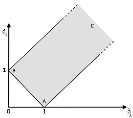
Figure 3: The weak turbulence equations are integrated over a domain such that ${\bf k}={\bf p}+{\bf q}$. The (gray) band corresponds to this domain for the normalized perpendicular wave vectors. Points A, B, and C (at infinity) are the regions of non locality.

$\bullet$ Case A:

$$\tilde{p}_{\perp} = 1+r\cos\alpha\,,$$ (82)

$$\tilde{q}_{\perp} = r\sin\alpha\,,$$ (83)

where $\alpha\in[\pi/4,3\pi/4]$ and $r\ll 1$. For this region, we find the convergence condition:

$$n+m > -3\,,$$ (84)

$$\tilde{n}+\tilde{m} > -4\,.$$ (85)

$\bullet$ Case B:

$$\tilde{p}_{\perp} = r\cos\alpha\,,$$ (86)

$$\tilde{q}_{\perp} = 1+r\sin\alpha\,,$$ (87)

where $\alpha\in[-\pi/4,\pi/4]$ and $r\ll 1$. For this region, we find the convergence condition:

$$n+m > -4\,,$$ (88)

$$\tilde{n}+\tilde{m} > -5\,.$$ (89)

$\bullet$ Case C:

$$\tilde{p}_{\perp} = {\tau_{2}-\tau_{1}\over 2}\,,$$ (90)

$$\tilde{q}_{\perp} = {\tau_{1}+\tau_{2}\over 2}\,,$$ (91)

where $-1<\tau_{1}<+1$ and $+1<\tau_{2}<+\infty$. For this region, we find the convergence condition:

$$n+m < -2\,,$$ (92)

$$\tilde{n}+\tilde{m} < -3\,.$$ (93)

The locality analysis for the parallel wave numbers does not lead to any new constrains. Thus, the convergence condition corresponds to the inequalities:

$$-3<n + m<-2\,,$$ (94)

$$-4<\tilde{n} + \tilde{m}<-3\,.$$ (95)

Appendix C Sign of magnetic helicity flux

The sign of the helicity flux may be investigated from the weak turbulence equation (74):

$$\partial_{t}{H_{k}}={\epsilon^{2}\over 32}\,\sum_{ss_{p}s_{q}}\int\left({\sin\theta_{k}\over k_{\perp}}\right)p_{\perp}|p_{\parallel}|\left({s_{q}q_{\perp}-s_{p}p_{\perp}\over k_{\parallel}}\right)^{2}(sk_{\perp}+s_{p}p_{\perp}+s_{q}q_{\perp})^{2}$$ (96)

$$\left[\left({q_{\perp}\over k_{\perp}}\right)^{n-1}\left|{q_{\parallel}\over k_{\parallel}}\right|^{m}\left(s-s_{p}\left({p_{\perp}\over k_{\perp}}\right)^{\tilde{n}}\left|{p_{\parallel}\over k_{\parallel}}\right|^{\tilde{m}}\right)-s_{q}\left({q_{\perp}\over k_{\perp}}\right)^{\tilde{n}}\left|{q_{\parallel}\over k_{\parallel}}\right|^{\tilde{m}}\left(1-\left({p_{\perp}\over k_{\perp}}\right)^{n-1}\left|{p_{\parallel}\over k_{\parallel}}\right|^{m}\right)\right]$$

$$C_{E}C_{H}k_{\perp}^{n+\tilde{n}-1}|k_{\parallel}|^{m+\tilde{m}+1}\left(1-\left({p_{\perp}\over k_{\perp}}\right)^{-n-\tilde{n}-6}\left|{p_{\parallel}\over k_{\parallel}}\right|^{-m-\tilde{m}-1}\right)$$

$$\delta(k_{\parallel}-p_{\parallel}-q_{\parallel})\,\delta(sk_{\perp}k_{\parallel}-s_{p}p_{\perp}p_{\parallel}-s_{q}q_{\perp}q_{\parallel})\,dp_{\perp}dq_{\perp}dp_{\parallel}dq_{\parallel}\,.$$

Additionally, we have (Zakharov et al., 1992):

$$\partial_{t}{H_{k}}=-\nabla\cdot{\bf P}=-{1\over k_{\perp}}{\partial(k_{\perp}P_{\perp})\over\partial k_{\perp}}-{\partial P_{\parallel}\over\partial k_{\parallel}}\,,$$ (97)

where ${\bf P}$ is the helicity flux vector , $P_{\perp}$ and $P_{\parallel}$ the perpendicular and parallel components of this flux vector (axisymmetric turbulence is assumed) respectively. We introduce the notations: $\tilde{p}_{\perp}\equiv p_{\perp}/k_{\perp}$, $\tilde{q}_{\perp}\equiv q_{\perp}/k_{\perp}$, $\tilde{p}_{\parallel}\equiv|p_{\parallel}|/|k_{\parallel}|$ and $\tilde{q}_{\parallel}\equiv|q_{\parallel}|/|k_{\parallel}|$ and obtain:

$$\partial_{t}{H_{k}}=\epsilon^{2}C_{E}C_{H}k_{\perp}^{n+\tilde{n}+4}|k_{\parallel}|^{m+\tilde{m}}I(m,n,\tilde{m},\tilde{n})\,,$$ (98)

with:

$$I(m,n,\tilde{m},\tilde{n})=$$ (99)

$${1\over 32}\,\sum_{ss_{p}s_{q}}\int\sqrt{1-\left({\tilde{p}_{\perp}^{2}+\tilde{q}_{\perp}^{2}-1\over 2\tilde{p}_{\perp}\tilde{q}_{\perp}}\right)^{2}}\,\tilde{p}_{\perp}\tilde{p}_{\parallel}\left(s_{q}\tilde{q}_{\perp}-s_{p}\tilde{p}_{\perp}\right)^{2}(s+s_{p}\tilde{p}_{\perp}+s_{q}\tilde{q}_{\perp})^{2}$$

$$\left[\tilde{q}_{\perp}^{n-1}\tilde{q}_{\parallel}^{m}\left(s-s_{p}\tilde{p}_{\perp}^{\tilde{n}}\tilde{p}_{\parallel}^{\tilde{m}}\right)-s_{q}\tilde{q}_{\perp}^{\tilde{n}}q_{\parallel}^{\tilde{m}}\left(1-\tilde{p}_{\perp}^{n-1}\tilde{p}_{\parallel}^{m}\right)\right]\left(1-\tilde{p}_{\perp}^{-n-\tilde{n}-6}\tilde{p}_{\parallel}^{-m-\tilde{m}-1}\right)$$

$$\delta(1-\tilde{p}_{\parallel}-\tilde{q}_{\parallel})\,\delta(s-s_{p}\tilde{p}_{\perp}\tilde{p}_{\parallel}-s_{q}\tilde{q}_{\perp}\tilde{q}_{\parallel})\,d\tilde{p}_{\perp}d\tilde{q}_{\perp}d\tilde{p}_{\parallel}d\tilde{q}_{\parallel}\,.$$

From the flux equation (97), we may have at constant $k_{\parallel}$:

$${\partial(k_{\perp}P_{\perp})\over\partial k_{\perp}}=-\epsilon^{2}C_{E}C_{H}k_{\perp}^{n+\tilde{n}+5}|k_{\parallel}|^{m+\tilde{m}}I(m,n,\tilde{m},\tilde{n})\,.$$ (100)

After an integration, we have the general relation:

$$P_{\perp}=-\epsilon^{2}C_{E}C_{H}k_{\perp}^{n+\tilde{n}+5}|k_{\parallel}|^{m+\tilde{m}}{I(m,n,\tilde{m},\tilde{n})\over n+\tilde{n}+6}\,.$$ (101)

The constant flux solution that we look for corresponds precisely to the cancellations of the denominator and the numerator $I$. This indeterminacy can be evaluated using L’Hospital’s rule; we find for this solution:

$$P_{\perp}=-\epsilon^{2}{C_{E}C_{H}\over k_{\perp}|k_{\parallel}|}A\,,$$ (102)

with:

$$A=\left({\partial I(m,n,\tilde{m},\tilde{n})\over\partial(n+\tilde{n}+6)}\right)_{n+\tilde{n}=-6,\,m+\tilde{m}=-1}=$$ (103)

$${1\over 32}\,\sum_{ss_{p}s_{q}}\int\sqrt{1-\left({\tilde{p}_{\perp}^{2}+\tilde{q}_{\perp}^{2}-1\over 2\tilde{p}_{\perp}\tilde{q}_{\perp}}\right)^{2}}\,\tilde{p}_{\perp}\tilde{p}_{\parallel}\left(s_{q}\tilde{q}_{\perp}-s_{p}\tilde{p}_{\perp}\right)^{2}(s+s_{p}\tilde{p}_{\perp}+s_{q}\tilde{q}_{\perp})^{2}$$ (104)

$$\ln(\tilde{p}_{\perp})\left[\tilde{q}_{\perp}^{n-1}\tilde{q}_{\parallel}^{m}\left(s-s_{p}\tilde{p}_{\perp}^{-n-6}\tilde{p}_{\parallel}^{-m-1}\right)-s_{q}\tilde{q}_{\perp}^{-n-6}q_{\parallel}^{-m-1}\left(1-\tilde{p}_{\perp}^{n-1}\tilde{p}_{\parallel}^{m}\right)\right]$$

$$\delta(1-\tilde{p}_{\parallel}-\tilde{q}_{\parallel})\,\delta(s-s_{p}\tilde{p}_{\perp}\tilde{p}_{\parallel}-s_{q}\tilde{q}_{\perp}\tilde{q}_{\parallel})\,d\tilde{p}_{\perp}d\tilde{q}_{\perp}d\tilde{p}_{\parallel}d\tilde{q}_{\parallel}\,.$$

In a similar way from the flux equation (97), we may have at constant $k_{\perp}$:

$${\partial P_{\parallel}\over\partial k_{\parallel}}=-\epsilon^{2}C_{E}C_{H}k_{\perp}^{n+\tilde{n}+4}|k_{\parallel}|^{m+\tilde{m}}I(m,n,\tilde{m},\tilde{n})\,.$$ (105)

After an integration, we find the general relation:

$$P_{\parallel}=-\epsilon^{2}C_{E}C_{H}k_{\perp}^{n+\tilde{n}+4}|k_{\parallel}|^{m+\tilde{m}+1}{I(m,n,\tilde{m},\tilde{n})\over m+\tilde{m}+1}\,.$$ (106)

As above, the constant flux solution corresponds to the cancellations of the denominator and $I$. Thanks to L’Hospital’s rule, we find:

$$P_{\parallel}=-\epsilon^{2}{C_{E}C_{H}\over k_{\perp}^{2}}B\,,$$ (107)

with (we introduce the solutions (56)–(57)):

$$B=\left({\partial I(m,n,\tilde{m},\tilde{n})\over\partial(m+\tilde{m}+1)}\right)_{n+\tilde{n}=-6,\,m+\tilde{m}=-1}=$$ (108)

$${1\over 32}\,\sum_{ss_{p}s_{q}}\int\sqrt{1-\left({\tilde{p}_{\perp}^{2}+\tilde{q}_{\perp}^{2}-1\over 2\tilde{p}_{\perp}\tilde{q}_{\perp}}\right)^{2}}\,\tilde{p}_{\perp}\tilde{p}_{\parallel}\left(s_{q}\tilde{q}_{\perp}-s_{p}\tilde{p}_{\perp}\right)^{2}(s+s_{p}\tilde{p}_{\perp}+s_{q}\tilde{q}_{\perp})^{2}$$ (109)

$$\ln(\tilde{p}_{\parallel})\left[\tilde{q}_{\perp}^{n-1}\tilde{q}_{\parallel}^{m}\left(s-s_{p}\tilde{p}_{\perp}^{-n-6}\tilde{p}_{\parallel}^{-m-1}\right)-s_{q}\tilde{q}_{\perp}^{-n-6}q_{\parallel}^{-m-1}\left(1-\tilde{p}_{\perp}^{n-1}\tilde{p}_{\parallel}^{m}\right)\right]$$

$$\delta(1-\tilde{p}_{\parallel}-\tilde{q}_{\parallel})\,\delta(s-s_{p}\tilde{p}_{\perp}\tilde{p}_{\parallel}-s_{q}\tilde{q}_{\perp}\tilde{q}_{\parallel})\,d\tilde{p}_{\perp}d\tilde{q}_{\perp}d\tilde{p}_{\parallel}d\tilde{q}_{\parallel}\,.$$

The combination of relations (102) and (107) gives in particular the flux ratio:

$${P_{\parallel}\over P_{\perp}}={k_{\parallel}\over k_{\perp}}{B\over A}\,,$$ (110)

which is small if $A$ and $B$ are of the same order. We see that the signs of the fluxes $P_{\perp}$ and $P_{\parallel}$ will be given by the signs of the constants $A$ and $B$ respectively (the constants $C_{E}$ and $C_{H}$ are taken positive).

References

• Alexandrova et al. (2009) Alexandrova, O., Saur, J., Lacombe, C., Mangeney, A., Mitchell, J., Schwartz, S. J. & Robert, P. 2009 Universality of Solar-Wind Turbulent Spectrum from MHD to Electron Scales. Phys. Rev. Lett. 103 (16), 165003.
• Banerjee et al. (2013) Banerjee, D., Ray, S. S., Sahoo, G. & Pandit, R. 2013 Multiscaling in Hall-Magnetohydrodynamic Turbulence: Insights from a Shell Model. Phys. Rev. Lett. 111 (17), 174501.
• Bhattacharjee (2004) Bhattacharjee, A. 2004 Impulsive Magnetic Reconnection in the Earth’s Magnetotail and the Solar Corona. Annu. Rev. Astron. Astrophys. 42, 365–384.
• Biskamp (2000) Biskamp, D. 2000 Magnetic Reconnection in Plasmas. Cambridge Univ. Press, Cambridge.
• Biskamp et al. (1996) Biskamp, D., Schwarz, E. & Drake, J. F. 1996 Two-Dimensional Electron Magnetohydrodynamic Turbulence. Phys. Rev. Lett. 76, 1264–1267.
• Boldyrev et al. (2013) Boldyrev, S., Horaites, K., Xia, Q. & Perez, J. C. 2013 Toward a Theory of Astrophysical Plasma Turbulence at Subproton Scales. Astrophys. J. 777, 41.
• Boldyrev & Perez (2012) Boldyrev, S. & Perez, J. C. 2012 Spectrum of Kinetic-Alfvén Turbulence. Astrophys. J. Lett. 758, L44.
• Bourouaine et al. (2012) Bourouaine, S., Alexandrova, O., Marsch, E. & Maksimovic, M. 2012 On Spectral Breaks in the Power Spectra of Magnetic Fluctuations in Fast Solar Wind between 0.3 and 0.9 AU. Astrophys. J. 749, 102.
• Bulanov et al. (1992) Bulanov, S. V., Pegoraro, F. & Sakharov, A. S. 1992 Magnetic reconnection in electron magnetohydrodynamics. Phys. Fluids B 4, 2499–2508.
• Cai et al. (2011) Cai, H.-B., Zhu, S.-P., Chen, M., Wu, S.-Z., He, X. T. & Mima, K. 2011 Magnetic-field generation and electron-collimation analysis for propagating fast electron beams in overdense plasmas. Phys. Rev. E 83 (3), 036408.
• Carbone (2012) Carbone, V. 2012 Scalings, Cascade and Intermittency in Solar Wind Turbulence. Space Sci. Rev. 172, 343–360.
• Chen et al. (2013) Chen, C. H. K., Boldyrev, S., Xia, Q. & Perez, J. C. 2013 Nature of Subproton Scale Turbulence in the Solar Wind. Phys. Rev. Lett. 110 (22), 225002.
• Cho (2011) Cho, J. 2011 Magnetic helicity conservation and inverse energy cascade in electron MHD wave packets. Phys. Rev. Lett. 106, 191104.
• Cho & Lazarian (2004) Cho, J. & Lazarian, A. 2004 The Anisotropy of Electron Magnetohydrodynamic Turbulence. Astrophys. J. Lett. 615, L41–L44.
• Cho & Lazarian (2009) Cho, J. & Lazarian, A. 2009 Simulations of Electron Magnetohydrodynamic Turbulence. Astrophys. J. 701, 236–252.
• Das (1999) Das, A. 1999 Nonlinear aspects of two-dimensional electron magnetohydrodynamics. Plasma Physics and Controlled Fusion 41, A531–A538.
• Das & Diamond (2000) Das, A. & Diamond, P. H. 2000 Theory of two-dimensional mean field electron magnetohydrodynamics. Phys. Plasmas 7, 170–177.
• Diamond et al. (2011) Diamond, P. H., Hasegawa, A. & Mima, K. 2011 Vorticity dynamics, drift wave turbulence, and zonal flows: a look back and a look ahead. Plasma Physics and Controlled Fusion 53 (12), 124001.
• Drake et al. (1994) Drake, J. F., Kleva, R. G. & Mandt, M. E. 1994 Structure of thin current layers: Implications for magnetic reconnection. Phys. Rev. Lett. 73, 1251–1254.
• Dreher et al. (2005) Dreher, J., Laveder, D., Grauer, R., Passot, T. & Sulem, P. L. 2005 Formation and disruption of Alfvénic filaments in Hall magnetohydrodynamics. Phys. Plasmas 12 (5), 052319.
• Frieman & Chen (1982) Frieman, E. A. & Chen, L. 1982 Nonlinear gyrokinetic equations for low-frequency electromagnetic waves in general plasma equilibria. Phys. Fluids 25, 502–508.
• Galtier (2003) Galtier, S. 2003 Weak inertial-wave turbulence theory. Phys. Rev. E (R) 68, 015301.
• Galtier (2006a) Galtier, S. 2006a Multi-scale Turbulence in the Inner Solar Wind. J. Low Temp. Physics 145, 59–74.
• Galtier (2006b) Galtier, S. 2006b Wave turbulence in incompressible Hall magnetohydrodynamics. J. Plasma Physics 72, 721–769.
• Galtier (2008) Galtier, S. 2008 von Kármán-Howarth equations for Hall magnetohydrodynamic flows. Phys. Rev. E 77 (1), 015302.
• Galtier (2014) Galtier, S. 2014 Theory of helical turbulence under fast rotation. Phys. Rev. E (R) 89, 041001.
• Galtier & Bhattacharjee (2003) Galtier, S. & Bhattacharjee, A. 2003 Anisotropic weak whistler wave turbulence in electron magnetohydrodynamics. Phys. Plasmas 10, 3065–3076.
• Galtier & Bhattacharjee (2005) Galtier, S. & Bhattacharjee, A. 2005 Anisotropic wave turbulence in electron MHD. Plasma Phys. Controlled Fusion 47, B691–B701.
• Galtier & Buchlin (2007) Galtier, S. & Buchlin, E. 2007 Multiscale Hall-Magnetohydrodynamic Turbulence in the Solar Wind. Astrophys. J. 656, 560–566.
• Galtier et al. (2001) Galtier, S., Nazarenko, S. V. & Newell, A. C. 2001 On wave turbulence in MHD. Nonlinear Proc. Geophys. 8, 141–150.
• Galtier et al. (2005) Galtier, S., Pouquet, A. & Mangeney, A. 2005 On spectral scaling laws for incompressible anisotropic magnetohydrodynamic turbulence. Phys. Plasmas 12 (9), 092310.
• Ghosh & Goldstein (1997) Ghosh, S. & Goldstein, M. L. 1997 Anisotropy in Hall MHD turbulence due to a mean magnetic field. J. Plasma Phys. 57, 129–154.
• Ghosh et al. (1996) Ghosh, S., Siregar, E., Roberts, D. A. & Goldstein, M. L. 1996 Simulation of high-frequency solar wind power spectra using Hall magnetohydrodynamics. J. Geophys. Res. 101, 2493–2504.
• Goldreich & Reisenegger (1992) Goldreich, P. & Reisenegger, A. 1992 Magnetic field decay in isolated neutron stars. Astrophys. J. 395, 250–258.
• Goldstein & Roberts (1999) Goldstein, M. L. & Roberts, D. A. 1999 Magnetohydrodynamic turbulence in the solar wind. Phys. Plasmas 6, 4154–4160.
• Hasegawa & Chen (1975) Hasegawa, A. & Chen, L. 1975 Kinetic process of plasma heating due to Alfvén wave excitation. Phys. Rev. Lett. 35, 370–373.
• Hirose et al. (2004) Hirose, A., Ito, A., Mahajan, S. M. & Ohsaki, S. 2004 Relation between Hall-MHD and the kinetic Alfvén wave. Phys. Lett. A 330, 474–480.
• Hori & Miura (2008) Hori, D. & Miura, H. 2008 Spectrum properties of hall mhd turbulence. Plasma and Fusion Research 3, S1053.
• Howes (2006) Howes, G. G. 2006 Limitations of Hall MHD as a model for turbulence in weakly collisional plasmas. Nonlin. Processes Geophys. 16, 219–232.
• Howes et al. (2008) Howes, G. G., Cowley, S. C., Dorland, W., Hammett, G. W., Quataert, E. & Schekochihin, A. A. 2008 A model of turbulence in magnetized plasmas: Implications for the dissipation range in the solar wind. J. Geophys. Res. (Space Physics) 113, 5103.
• Howes & Quataert (2010) Howes, G. G. & Quataert, E. 2010 On the Interpretation of Magnetic Helicity Signatures in the Dissipation Range Of Solar Wind Turbulence. Astrophys. J. Lett. 709, L49–L52.
• Hunana et al. (2011) Hunana, P., Laveder, D., Passot, T., Sulem, P. L. & Borgogno, D. 2011 Reduction of Compressibility and Parallel Transfer by Landau Damping in Turbulent Magnetized Plasmas. Astrophys. J. 743, 128.
• Karimabadi et al. (2013) Karimabadi, H., Roytershteyn, V., Wan, M., Matthaeus, W. H., Daughton, W., Wu, P., Shay, M., Loring, B., Borovsky, J., Leonardis, E., Chapman, S. C. & Nakamura, T. K. M. 2013 Coherent structures, intermittent turbulence, and dissipation in high-temperature plasmas. Phys. Plasmas 20 (1), 012303.
• Kingsep et al. (1990) Kingsep, A.S., Chukbar, K.V. & Yankov, V.V. 1990 Review of plasma physics. Consultant bureau, New York, vol. 16.
• Kiyani et al. (2009) Kiyani, K. H., Chapman, S. C., Khotyaintsev, Y. V., Dunlop, M. W. & Sahraoui, F. 2009 Global Scale-Invariant Dissipation in Collisionless Plasma Turbulence. Phys. Rev. Lett. 103 (7), 075006.
• Lukin (2009) Lukin, V. S. 2009 Stationary nontearing inertial scale electron magnetohydrodynamic instability. Phys. Plasmas 16 (12), 122105.
• Lvov et al. (2004) Lvov, Y.V., Polzin, K.L. & Tabak, E.G. 2004 Energy spectra of the ocean’s internal wave field: theory and observations. Phys. Rev. Lett. 92 (12), 128501.
• Lyutikov (2013) Lyutikov, M. 2013 Electron magnetohydrodynamics: Dynamics and turbulence. Phys. Rev. E 88, 053103.
• Mandt et al. (1994) Mandt, M. E., Denton, R. E. & Drake, J. F. 1994 Transition to whistler mediated magnetic reconnection. Geophys. Res. Lett. 21, 73–76.
• Martin et al. (2012) Martin, L.N., Dmitruk, P. & Gomez, D.O. 2012 Energy spectrum, dissipation, and spatial structures in reduced Hall magnetohydrodynamic. Phys. Plasmas 19, 052305.
• Matthaeus & Goldstein (1982) Matthaeus, W. H. & Goldstein, M. L. 1982 Measurement of the rugged invariants of magnetohydrodynamic turbulence in the solar wind. J. Geophys. Res. 87, 6011–6028.
• Matthaeus et al. (2014) Matthaeus, W. H., Oughton, S., Osman, K. T., Servidio, S., Wan, M., Gary, S. P., Shay, M. A., Valentini, F., Roytershteyn, V., Karimabadi, H. & Chapman, S. C. 2014 Nonlinear and Linear Timescales near Kinetic Scales in Solar Wind Turbulence. ArXiv 1404.6569 .
• Meyrand & Galtier (2010) Meyrand, R. & Galtier, S. 2010 A Universal Law for Solar-wind Turbulence at Electron Scales. Astrophys. J. 721, 1421–1424.
• Meyrand & Galtier (2012) Meyrand, R. & Galtier, S. 2012 Spontaneous Chiral Symmetry Breaking of Hall Magnetohydrodynamic Turbulence. Phys. Rev. Lett. 109 (19), 194501.
• Meyrand & Galtier (2013) Meyrand, R. & Galtier, S. 2013 Anomalous $k_{\perp}^{-8/3}$ spectrum in electron magnetohydrodynamic turbulence. Phys. Rev. Lett. 111, 264501.
• Mininni et al. (2007) Mininni, P. D., Alexakis, A. & Pouquet, A. 2007 Energy transfer in Hall-MHD turbulence: cascades, backscatter, and dynamo action. J. Plasma Physics 73, 377–401.
• Nazarenko (2011) Nazarenko, S., ed. 2011 Wave Turbulence, Lecture Notes in Physics, Berlin Springer Verlag, vol. 825.
• Ng et al. (2003) Ng, C. S., Bhattacharjee, A., Germaschewski, K. & Galtier, S. 2003 Anisotropic fluid turbulence in the interstellar medium and solar wind. Phys. Plasmas 10, 1954–1962.
• Passot et al. (2014) Passot, T., Henri, P., Laveder, D. & Sulem, P.L. 2014 Fluid simulations of ion scale plasmas with weakly distorted magnetic field. Submitted 000, 000.
• Pouquet et al. (1976) Pouquet, A., Frisch, U. & Leorat, J. 1976 Strong MHD helical turbulence and the nonlinear dynamo effect. J. Fluid Mech. 77, 321–354.
• Rousculp & Stenzel (1997) Rousculp, C. L. & Stenzel, R. L. 1997 Helicity Injection by Knotted Antennas into Electron Magnetohydrodynamical Plasmas. Phys. Rev. Lett. 79, 837–840.
• Rudakov et al. (2011) Rudakov, L., Mithaiwala, M., Ganguli, G. & Crabtree, C. 2011 Linear and nonlinear Landau resonance of kinetic Alfvén waves: Consequences for electron distribution and wave spectrum in the solar wind. Phys. Plasmas 18 (1), 012307.
• Sahraoui et al. (2012) Sahraoui, F., Belmont, G. & Goldstein, M. L. 2012 New Insight into Short-wavelength Solar Wind Fluctuations from Vlasov Theory. Astrophys. J. 748, 100.
• Sahraoui et al. (2007) Sahraoui, F., Galtier, S. & Belmont, G. 2007 On waves in incompressible Hall magnetohydrodynamics. J. Plasma Physics 73, 723–730.
• Sahraoui et al. (2010) Sahraoui, F., Goldstein, M. L., Belmont, G., Canu, P. & Rezeau, L. 2010 Three Dimensional Anisotropic k Spectra of Turbulence at Subproton Scales in the Solar Wind. Phys. Rev. Lett. 105 (13), 131101.
• Sahraoui et al. (2013) Sahraoui, F., Huang, S. Y., Belmont, G., Goldstein, M. L., Rétino, A., Robert, P. & De Patoul, J. 2013 Scaling of the Electron Dissipation Range of Solar Wind Turbulence. Astrophys. J. 777, 15.
• Schekochihin et al. (2009) Schekochihin, A. A., Cowley, S. C., Dorland, W., Hammett, G. W., Howes, G. G., Quataert, E. & Tatsuno, T. 2009 Astrophysical Gyrokinetics: Kinetic and Fluid Turbulent Cascades in Magnetized Weakly Collisional Plasmas. Astrophys. J. Suppl. 182, 310–377.
• Sentoku et al. (2003) Sentoku, Y., Mima, K., Kaw, P. & Nishikawa, K. 2003 Anomalous Resistivity Resulting from MeV-Electron Transport in Overdense Plasma. Phys. Rev. Lett. 90 (15), 155001.
• Shaikh & Zank (2005) Shaikh, D. & Zank, G. P. 2005 Driven dissipative whistler wave turbulence. Phys. Plasmas 12 (12), 122310.
• Shepherd & Cassak (2010) Shepherd, L. S. & Cassak, P. A. 2010 Comparison of Secondary Islands in Collisional Reconnection to Hall Reconnection. Phys. Rev. Lett. 105 (1), 015004.
• Smith et al. (2006) Smith, C. W., Hamilton, K., Vasquez, B. J. & Leamon, R. J. 2006 Dependence of the Dissipation Range Spectrum of Interplanetary Magnetic Fluctuations on the Rate of Energy Cascade. Astrophys. J. Lett. 645, L85–L88.
• Stenzel & Urrutia (1996) Stenzel, R. L. & Urrutia, J. M. 1996 Helicity and Transport in Electron MHD Heat Pulses. Phys. Rev. Lett. 76, 1469–1472.
• Stenzel et al. (1995) Stenzel, R. L., Urrutia, J. M. & Rousculp, C. L. 1995 Helicities of Electron Magnetohydrodynamic Currents and Fields in Plasmas. Phys. Rev. Lett. 74, 702–705.
• Tessein et al. (2009) Tessein, J. A., Smith, C. W., MacBride, B. T., Matthaeus, W. H., Forman, M. A. & Borovsky, J. E. 2009 Spectral Indices for Multi-Dimensional Interplanetary Turbulence at 1 AU. Astrophys. J. 692, 684–693.
• Voitenko (1998) Voitenko, Y. M. 1998 Three-wave coupling and weak turbulence of kinetic Alfvén waves. J. Plasma Phys. 60, 515–527.
• Zakharov et al. (1992) Zakharov, V. E., L’Vov, V. S. & Falkovich, G. 1992 Kolmogorov spectra of turbulence I: Wave turbulence. Springer Series in Nonlinear Dynamics, Berlin.