Peltier Cooling of Fermionic Quantum Gases

Abstract

We propose a cooling scheme for fermionic quantum gases, based on the principles of the Peltier thermoelectric effect and energy filtering. The system to be cooled is connected to another harmonically trapped gas acting as a reservoir. The cooling is achieved by two simultaneous processes: (i) the system is evaporatively cooled and (ii) cold fermions from deep below the Fermi surface of the reservoir are injected below the Fermi level of the system, in order to fill the ’holes’ in the energy distribution. This is achieved by a suitable energy dependence of the transmission coefficient connecting the system to the reservoir. The two processes can be viewed as simultaneous evaporative cooling of particles and holes. We show that both a significantly lower entropy per particle and faster cooling rate can be achieved than by using only evaporative cooling.

Introduction

The Peltier effect is a reversible thermoelectric phenomenon, in which heat is absorbed or produced at the junction of two materials forming a circuit in which a current is circulated Goldsmid (2009). Peltier cooling modules based on this effect are used for a variety of applications ranging from wine coolers to the cooling of electronic devices. The basic principle of a Peltier module is schematized on Fig. 1(c). It consists of two materials with Seebeck coefficients of opposite signs (p-type and n-type) arranged as indicated. A heat (entropy) current flows in both materials from the cold side to the hot side. Microscopically, this heat current corresponds to a flow of energetic electrons in the n-branch: hot electrons above Fermi level are ‘evaporated’ out of the cold plate. Similarly, a hole current flows in the same direction in the p-branch, so that holes below Fermi level are being filled. Both processes lead to a rectification of the energy distribution of electrons in the cold plate (Fig. 1(b)), and hence to a decrease of its entropy.

In the context of mesoscopic electronic systems, thermoelectric effects as well as thermal properties and refrigeration have recently been the focus of renewed interest Entin-Wohlman et al. (2010); Sánchez and Büttiker (2011); Giazotto et al. (2006). The cooling of low-dimensional nanostructures has been proposed Edwards et al. (1993); Jordan et al. (2013); Whitney (2014) and experimentally realized Prance et al. (2009); Timofeev et al. (2009); Giazotto et al. (2006), for example by engineering a proper energy dependence of the transmission coefficients using quantum dots.

In the field of cold atomic Fermi gases, reaching lower temperatures is currently one of the most urgent challenges. Typically, the cooling of these gases is achieved using laser cooling followed by evaporative cooling Ketterle and van Druten (1996); Pethick and Smith (2008). Quantum degeneracy and very low absolute temperatures of the order a few hundred nano-Kelvin are typically reached with these techniques, leading to the observation of many remarkable phenomena such as the BCS-BEC crossover Ketterle et al. (2008). However, the entropy per particle, which is the relevant quantity in these well isolated fermionic gases, is still too large ($T/T_{F}\approx 0.1$) McKay and DeMarco (2011) to investigate many of the most intriguing quantum effects such as the quantum Hall effect Cooper (2008), low-temperature transport, spin liquids Lewenstein et al. (2012), or even antiferromagnetic order in the Hubbard model Jördens et al. (2010); Bloch et al. (2008).

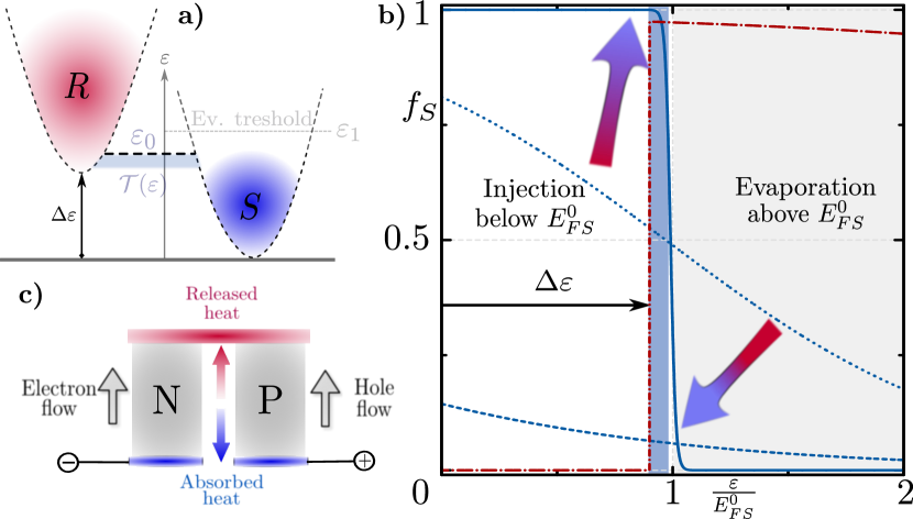
Figure 1: (Color online): a) Sketch of the proposed Peltier cooling scheme: atoms are injected from deep energy levels of the reservoir cloud ($R$) into the system cloud ($S$) just below the Fermi level through a channel with an energy-dependent transmission $\mathcal{T}(\varepsilon)$. Additionally, the system is submitted to evaporative cooling with a fixed evaporation threshold $\varepsilon_{1}$ above Fermi level, removing hot particles. b) Evolution of the Fermi distribution of the system at three stages during the cooling process: initial (dashed blue curve, $T_{S}\approx T_{FS}$), intermediate (blue dotted curve, $T_{S}=0.3T_{FS}$) and final (solid blue curve, $T_{S}=0.02T_{FS}$). The evolution, indicated by arrows, is calculated (see text) for $\varepsilon_{1}=1.05E^{0}_{FS}$, $\gamma_{ev}\tau_{0}=1/16$, $\varepsilon_{0}=0.99E^{0}_{FS}$, $\Delta\varepsilon=0.96E^{0}_{FS}$ and $E^{0}_{FS}=0.25E^{0}_{FR}$. The blue and grey shaded regions indicate the injection and evaporation energy windows, respectively. The dashed-dotted curve is the final distribution of the reservoir. c) Sketch of a Peltier cooling module. The $n$-like and $p$-like thermoelectric materials ensure the transport of low energy (electrons) and high energy (holes) particles, which thus carry heat from the cold (blue) to the hot (red) region.

Here, we propose an efficient cooling scheme for atomic Fermi gases which uses the Peltier effect in synergy with evaporative cooling. Our proposed setup is based on thermoelectric effects Brantut et al. (2013); Grenier et al. (2012); Hazlett et al. (2013); Rancon et al. (2013); Papoular et al. (2012, 2014); Sidorenkov et al. (2013); Kim and Huse (2012); Wong et al. (2012); Karpiuk et al. (2012) and is displayed on Fig. 1(a). Two clouds of fermions, a reservoir $R$ and a system $S$ to be cooled, are prepared in harmonic traps. The initial Fermi energies of the two gases are $E^{0}_{F,R/S}=h\bar{\nu}(3N_{R/S})^{1/3}$, with $\bar{\nu}$ the average trapping frequency  and $N_{R}$, $N_{S}$ the atom numbers ($N_{R}>N_{S}$). The lowest energy level of the reservoir is offset by $\Delta\varepsilon\geq 0$ as compared to that of the system. Two processes are implemented in order to lower the entropy of the system. The first one is evaporative cooling at a rate $\Gamma_{ev}$ applied to particles with energy higher than a threshold $\varepsilon_{1}$, chosen above the Fermi level $E^{0}_{FS}$. The second simultaneous process is the injection of fermions from the reservoir into the system below the system’s Fermi level which can be viewed as an ‘evaporation’ of holes.

This is achieved by connecting the traps by a constriction Brantut et al. (2012) characterized by an energy-dependent transmission $\mathcal{T}(\varepsilon)$. In an ideal setup, the transmission is chosen to have a box-like dependence on energy: any state with energy above $\Delta\varepsilon$ and below a threshold $\varepsilon_{0}$ located just below the Fermi level of the system is perfectly transmitted (Fig. 1(a)).

The combination of these two processes, the evaporative cooling and the injection of fermions below the Fermi surface, induces an efficient cooling. This can be seen from the time evolution of the energy distribution displayed on Fig. 1(b). Starting initially from a broad hot distribution, it evolves towards a rectified distribution with a sharp drop at the Fermi level, characteristic of a low temperature. The parameters of the cooling process can be chosen, such that the atom number in the system changes only slightly, since the atom losses from evaporative cooling can be compensated by the injection of the reservoir atoms. At the same time, the reservoir is heated and looses atoms. However, the bottom of the energy distribution of the reservoir remains filled (Fig. 1(b)), ensuring an efficient injection of cool particles. The cooling process stops when the system energy distribution becomes equal to the reservoir distribution in the transmission window. We show below that both the final entropy per atom and the cooling rate are improved in comparison to evaporative cooling only, by approximately a factor of four.

Model of the cooling process

We describe the process in terms of coupled rate equations for the distribution functions $f_{S}$ and $f_{R}$. We assume that thermalization in the system and in the reservoir is fast, so that they can be considered to be in thermodynamic equilibrium. Under this assumption, the particle current leaving the reservoir is given by the Landauer formula:

$$I_{N} = \frac{1}{h}\int\textrm{d}\varepsilon\;\mathcal{T}(\varepsilon)\left[f_{R}(\varepsilon)-f_{S}(\varepsilon)\right]$$

$$= -\int\textrm{d}\varepsilon g_{R}(\varepsilon)\frac{df_{R}}{dt}(\varepsilon)=\int\textrm{d}\varepsilon g_{S}(\varepsilon)\frac{df_{S}}{dt}(\varepsilon)\,.$$

In this expression, $g_{R}(\varepsilon)=\frac{(\varepsilon-\Delta\varepsilon)^{2}}{3(h\bar{\nu})^{3}}\vartheta(\epsilon-\Delta\varepsilon)$ and $g_{S}(\varepsilon)=\frac{\varepsilon^{2}}{{3(h\bar{\nu})^{3}}}\vartheta(\varepsilon)$ are the density of states in the reservoir and in the system, with $\vartheta$ the Heaviside function. The coupled evolution of the two distribution functions is thus given by :

$$g_{R}(\varepsilon)\frac{df_{R}(\varepsilon)}{dt} = -\frac{\mathcal{T}(\varepsilon)}{h}\left[f_{R}-f_{S}\right](\varepsilon)$$ (1)

$$g_{S}(\varepsilon)\frac{df_{S}(\varepsilon)}{dt} = \frac{\mathcal{T}(\varepsilon)}{h}\left[f_{R}-f_{S}\right](\varepsilon)-\Gamma_{ev}(\varepsilon)g_{S}(\varepsilon)f_{S}(\varepsilon)\,,$$ (2)

In the second equation, the effect of evaporation has been included as a leak of high energy particles above a fixed energy threshold $\varepsilon_{1}$, with an energy independent rate $\Gamma_{ev}(\varepsilon)=\gamma_{ev}\vartheta(\varepsilon-\varepsilon_{1})$ Ketterle and van Druten (1996). Since $\mathcal{T}(\varepsilon)$ is dimensionless, the typical time-scale that rules the time-evolution in these equations is $\tau_{0}=hg_{S}(E^{0}_{FS})=h\left(E^{0}_{FS}\right)^{2}/3(h\bar{\nu})^{3}$. This is the compressibility divided by the ‘conductance’ quantum, which has been identified as the time-scale for the particle transport in previous experiments Brantut et al. (2012, 2013).

In principle the scattering of the atoms has to be taken into account in the evolution equations. However, since we assume the scattering to be the fastest time-scale in the problem, we take it into account as an instantaneous re-thermalization. The evolution of the system is implemented by time-evolving the equations (1) and (2) for a small time step $\delta t$. From the particle numbers $N_{S,R}(t+\delta t)$ and energies $E_{S,R}(t+\delta t)$ one obtains new values of the chemical potentials $\mu_{S,R}$ and temperatures $T_{S,R}$ assuming thermodynamic equilibrium for a non-interacting gas. The resulting equilibrium Fermi functions $f_{S}(t+\delta t,\varepsilon)$ and $f_{R}(t+\delta t,\varepsilon)$ are subsequently evolved using the rate equations and the entire procedure is repeated. This description of cooling is in line with the pulsed approach of evaporation developed for example in Ref. Davis et al. (1995); Ketterle and van Druten (1996). The time-step $\delta t$ is chosen small enough, such that it does not affect the resulting evolution.

Unless specified, a transmission of the form $\mathcal{T}(\varepsilon)=\vartheta(\epsilon_{0}-\varepsilon)$ will be considered. This means that only states in the energy window $\varepsilon\in[\Delta\varepsilon,\varepsilon_{0}]$ can be transmitted (‘box-like’ transmission). As recently pointed out for electronic mesoscopic systems Whitney (2014) and further discussed in the last section, this transmission is the optimal choice to achieve the best cooling performances. To summarize, the scheme involves three characteristic energy thresholds: $\Delta\varepsilon\leq\varepsilon_{0}\leq\varepsilon_{1}$, corresponding respectively to the energy offset between $R$ and $S$, the maximum injection energy into $S$, and the minimum evaporation energy out of $S$.

Results and comparison to evaporative cooling

In the following we demonstrate the potential of the proposed Peltier cooling scheme by comparing it to commonly used evaporative cooling. We focus on the reachable entropy per particle and on the cooling rate. The entropy per particle $s$ in a trapped non-interacting Fermi-gas is related to the ratio $T/T_{F}$ by $s=\frac{\pi^{2}k_{B}}{2}\frac{T}{T_{F}}$ at low temperature, so that we use equivalently $s$ or $T/T_{F}$ below. The evolution of the entropy per particle is shown in the upper panel of Fig. 2. Assuming that the two gases are first prepared from a single cloud by evaporative cooling, we used a typically reached entropy per particle of $T/T_{F}=0.25$ as an initial value (with $T_{F}$ the Fermi temperature of the total cloud). Initially, the ratio of the atom numbers between the system and the reservoir is chosen such that $E^{0}_{FS}/E^{0}_{FR}=N_{S}/N_{R}=0.25$, which leads to the initial entropy per atom of $T_{S}/T_{FS}\simeq 1.07$ and $T_{R}/T_{FR}\simeq 0.27$. For the results in Fig. 2 we have chosen the evaporation threshold $\varepsilon_{1}=1.05E^{0}_{FS}$, the maximal transmission energy $\varepsilon_{0}=0.99E^{0}_{FS}$, i.e. close to the target Fermi energy (which is the initial one) and the chemical potential bias $\Delta\varepsilon=0.96E^{0}_{FS}$. The evaporation rate is chosen to be $\gamma_{ev}\tau_{0}=1/16$. Fig. 2 shows that a very efficient reduction of the entropy per particle to a value of approximately $T_{S}/T_{FS}\approx 0.02$ is achieved within a short time-scale. At longer times, a slight rise in the entropy per particle sets in. The number of particles in the system is approximately constant with a slight increase at short times. This increase in the atom number in the system shows that during this time, the injection of fermions from the reservoir is particularly efficient. This increase is reduced by a dominating evaporation at intermediate times, until a quite stable state is reached at longer times.

In experimental setups, various heating mechanisms such as spontaneous emission Foot (2005), as well as particle losses, can limit drastically the lowest entropy that can be reached. The cooling process will stop being efficient when the cooling rate becomes comparable to the heating/emission rate, and it is therefore important to compare these two rates. To this purpose, we define the cooling rate $\eta$ as the time derivative of the entropy per particle : $\eta(t)=-\frac{ds_{S}(t)}{dt}\,,$ and display it in Fig. 3 versus the corresponding value of $T_{S}(t)/T_{FS}(t)$. The horizontal dashed line stands for a typical value of the experimental heating rate. From this plot, one can directly read off the entropy per particle which can be reached (here about $0.03T_{S}/T_{FS}$) in the presence of this heating rate.

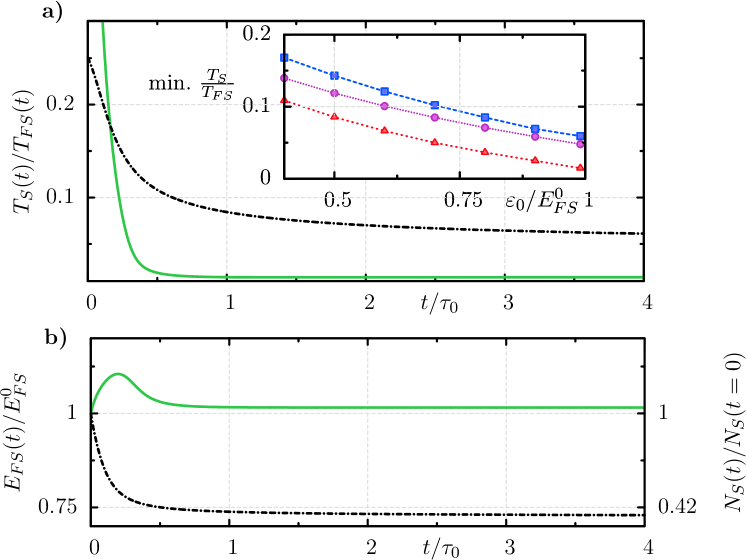
Figure 2: (Color online): Evolution during the cooling process of a) the entropy per particle $T_{S}(t)/T_{FS}(t)$ and b) the Fermi energy $E_{FS}(t)$ (left axis) and particle number $N_{S}(t)$ (right axis). The solid curves are for the Peltier cooling with $E^{0}_{FS}/E^{0}_{FR}=1/4$ and $\varepsilon_{1}=1.05E^{0}_{FS}$, $\gamma_{ev}\tau_{0}=1/16$, $\varepsilon_{0}=0.99E^{0}_{FS}$, $\Delta\varepsilon=0.96E^{0}_{FS}$. The dashed-dotted curves are for evaporative cooling only, with an initial particle number $N=N_{S}+N_{R}$ and $\varepsilon_{1}=1.05E_{F}$. Inset: minimum entropy per particle achieved by Peltier cooling, as a function of $\varepsilon_{0}$, for : $\varepsilon_{1}=1.05E^{0}_{FS}$ and $(\epsilon_{0}-\Delta\varepsilon)/E^{0}_{FS}=3\%$ (red triangles), $20\%$ (purple circles) and $\varepsilon_{1}=1.5E^{0}_{FS}$, $(\epsilon_{0}-\Delta\varepsilon)/E^{0}_{FS}=3\%$ (blue squares).

To assess the usefulness of our cooling scheme, we compare it to evaporative cooling applied to the total initial cloud with $N=N_{R}+N_{S}$ with the same initial temperature, here $T/T_{F}=0.25$, and the same evaporation threshold relative to the Fermi energy $\varepsilon_{1}=1.05E^{0}_{F}$, where $E^{0}_{F}$ is the initial Fermi energy of the total cloud. Since for the evaporative cooling no separation of the total cloud in two subclouds is performed we use the index $S$ to label the quantities of the entire cloud. We see from Fig. 2 that at short times, the entropy reached by the proposed cooling scheme is much lower than the one reached by evaporative cooling. So if one aims at reaching a given low value of $T/T_{F}$, this value is reached faster with the proposed scheme. At the same time one sees that the particle number during the evaporative cooling is reducing drastically to about 40 percent of its initial value . At infinite times, the evaporative cooling would empty the reservoir and during this process reach lower and lower entropy per particles. Nevertheless, as cooling takes place, evaporation is less and less efficient, and the cooling rate of evaporation slows down considerably: as seen on Fig. 3 the cooling rate for the Peltier scheme is much larger than for the evaporative scheme, at a given entropy per particle. Due to this faster cooling rate, the temperatures which can be reached in the presence of heating or spontaneous emission are much deeper in the degenerate regime when using the Peltier cooling. As seen on Fig. 3, for the chosen heating rate, an entropy per particle of order $0.03T_{S}/T_{FS}$ is reached using the Peltier scheme, in contrast to $0.13T_{S}/T_{FS}$ using evaporative cooling only.

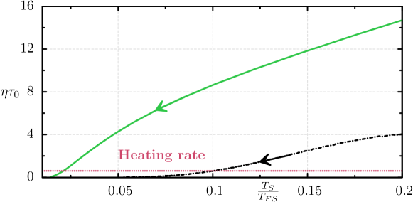
Figure 3: (Color online): Dimensionless cooling rate $\eta(t)\tau_{0}$ as a function of $T_{S}/T_{FS}$, for the same parameters as in Fig. 2. The black dashed curve is for evaporative cooling only. Arrows indicate the direction of the time evolution. The horizontal (red) dotted line indicates a typical heating rate limiting these cooling processes.

The inset of Fig. 2(a) illustrates how the minimum of the entropy per particle depends on the parameters of the setup. The injection energy window $\varepsilon_{0}-\Delta\varepsilon$ should be relatively narrow to obtain a low entropy, but broad enough to allow for a fast cooling. Having in addition an evaporation threshold as close as possible to the target Fermi energy also improves the final value of the entropy per particle. The cooling scheme could further be optimized by changing some of the parameters in a time-dependent manner, as commonly done for the threshold in evaporative cooling. For the sake of simplicity, we kept all parameters constant in our study.

Possible implementations of the energy-dependent transmission

The Peltier cooling scheme relies on a transmission coefficient ensuring proper ‘energy filtering’ between the two gases. We now discuss possible realizations of appropriate transmission functions with state-of-the-art projection techniques Zimmermann et al. (2011); Bakr et al. (2009); Sherson et al. (2010). We consider mainly two distinct forms (see Fig. 4(b)). First, a narrow (delta-function like) transmission in energy which can for example be realized by a single resonant level (or many in parallel) Datta (1997). Such a narrow energy filter Mahan and Sofo (1996), has been predicted to achieve the maximization of the cooling efficiency or equivalently of the thermoelectric figure of merit. Second, an approximately box-like transmission realized by two such resonant levels in series as discussed in the mesoscopics context Whitney (2014); Thomas and Flindt (2014). Such a box-like transmission with a finite width in energy is expected to show the maximum cooling power and best cooling rate (see Ref. Whitney (2014) and supplementary material Sup ).

The results for the cooling rates as a function of $T_{S}/T_{FS}$ are displayed in Fig. 4(a). As predicted, the idealized box-like transmission (solid green line) allows for reaching a very low temperature with a fast cooling rate. Two quantum dots connected in series (blue dotted curve in Fig. 4(a)) realize a good approximation to the box-like transmission and achieve a final entropy per particle which is only slightly higher. We also considered a single resonant level (red dash-dotted curve), with a width such that a low final entropy comparable to that of the idealized box is achieved. In contrast to the latter, this leads to a much slower cooling rate, comparable to that of evaporative cooling . Only in the final cooling stage, when the entropy per particle is low, does the cooling rate of the single resonant level become comparable to that of the ideal box. This low cooling rate can to some extent be overcome by using many resonant levels in parallel (orange dashed curve): a fast initial cooling is then observed, comparable to that of the idealized box, with only a slight increase of the minimal entropy per particle which can be reached. In summary, we have identified two different ways of realizing efficient cooling, either by connecting relatively broad resonant levels in series, or by using a large number of narrow resonant levels in parallel. The attainable values of $T_{S}/T_{FS}$ remain in all considered cases significantly better than what can be achieved from evaporation only.

Figure 4: (Color online) a) : Dimensionless cooling rate $\eta(t)\tau_{0}$ as a function of $T_{S}/T_{FS}$, for $\Delta\varepsilon=0.96E^{0}_{FS}$ and various transmissions centered at $\varepsilon_{0}=0.99E^{0}_{FS}$ (the other parameters are taken as in Fig. 2): The (red) dot-dashed and (orange) dashed curve correspond to a single and 100 parallel resonant level(s), respectively, with $\Gamma=2\cdot 10^{-4}E^{0}_{FS}$. The (blue) dotted curve is for two resonant levels in series of width $\Gamma=0.3E^{0}_{FS}$ and the (green) solid curve is for an ideal box transmission. (Black) dashed-dotted curve shows the evaporative cooling only. b): The corresponding energy-dependent transmission coefficients. The grey area indicates states above $\varepsilon_{1}$, while the blue one indicates those below $\Delta\varepsilon$, which do not participate to transport.

Conclusion

In this article, we have introduced a Peltier cooling scheme for fermionic gases, which combines conventional evaporation with energy-selective injection of particles. In a nutshell, this scheme can be described as a simultaneous evaporative cooling of particles and holes. We have proposed different realizations of the proper energy filtering between the reservoir and the cooled system, in line with the recent development of mesoscopic-like channels in cold atom gases Brantut et al. (2012); Thywissen et al. (1999). The proposed scheme achieves fast and efficient cooling down to temperatures deep in the quantum degenerate regime, a much desired current goal in the field of atomic fermion gases. The present work also demonstrates that the recent fundamental studies of coupled particle and entropy transport in cold atomic gases Brantut et al. (2013); Grenier et al. (2012); Hazlett et al. (2013); Rancon et al. (2013); Papoular et al. (2012, 2014); Sidorenkov et al. (2013); Kim and Huse (2012); Wong et al. (2012); Karpiuk et al. (2012) may also have useful implications for further experimental developments of the field.

Supplementary material for : ’Peltier Cooling of Fermionic Quantum Gases’

I Derivation of the main equations

Equations (1) and (2) in the main text rule the evolution of the distribution functions $f_{R}$ and $f_{S}$ in the reservoir and system respectively, under the influence of an energy dependent coupling represented by a transmission probability $\mathcal{T}(\varepsilon)$ and a ’leak’ of high energy particles representing the effect of evaporation.
The starting point to derive these equations is the balance of particle currents :

$$\dot{N_{R}} = I_{S\rightarrow R}-I_{R\rightarrow S}$$ (3)

$$\dot{N_{S}} = I_{R\rightarrow S}-I_{S\rightarrow R}-I_{evaporation}\,$$ (4)

which expresses the variation of the particle numbers in the system $S$ and reservoir $R$. Note that the evaporation which acts on the system leads to particle losses, such that the total particle number is not conserved. The Landauer formula gives the expression for the current flow between $S$ and $R$ :

$$I_{tot}=I_{S\rightarrow R}-I_{R\rightarrow S}=\frac{1}{h}\int d\varepsilon\,\mathcal{T}(\varepsilon)\,\left[f_{S}(\varepsilon,t)-f_{R}(\varepsilon,t)\right]\,.$$ (5)

The distributions fulfill the following relations :

$$\int d\varepsilon\,g_{S,R}(\varepsilon)\,f_{S,R}(\varepsilon,t) = N_{S,R}(t)$$ (6)

$$\int d\varepsilon\,\varepsilon\,g_{S,R}(\varepsilon)\,f_{S,R}(\varepsilon,t) = E_{S,R}(t)\,$$ (7)

where $N_{S,R}$ and $E_{S,R}$ are the particle number and energy in $S,R$ at time $t$.

The evaporation term has the following expression :

$$I_{evaporation}=\int d\varepsilon\,g_{S}(\varepsilon)\,f_{S}(\varepsilon)\,\Gamma_{ev}(\varepsilon)\,,$$ (8)

with $\Gamma_{ev}(\varepsilon)=\gamma_{ev}\theta(\varepsilon-\varepsilon_{1})$, representing the evaporation above a fixed threshold $\varepsilon_{1}$ at a rate $\gamma_{ev}$.

Finally, expressing the variation of particle number in $S$ and $R$ as

$$\dot{N}_{S,R}=\int d\varepsilon\,g_{S,R}(\varepsilon)\,\frac{df_{S,R}(t)}{dt}(\varepsilon)$$ (9)

gives the expressions (1) and (2) of the main text.

II Maximization of power factor

In the linear response regime, one can provide a quantitative explanation for the optimization of the cooling efficiency provided by a box-like transmission. The arguments that we will develop are similar to those presented in Ref.  Whitney (2014) in the mesoscopic context which covers also the nonlinear regime.

Here, we assume the response to be linear and search for the energy dependent transmission probability $\mathcal{T}(\varepsilon)$ that optimizes the power factor $\mathcal{P}=\alpha^{2}G$ MacDonald (2006), where $\alpha$ is the Seebeck coefficient and $G$ the conductance, given by :

$$G = \frac{1}{h}\int_{0}^{\infty}d\varepsilon\,\mathcal{T}(\varepsilon)\left(-\frac{\partial f}{\partial\varepsilon}\right)$$ (10)

$$\alpha = \frac{1}{T}\frac{\int_{0}^{\infty}d\varepsilon\,\mathcal{T}(\varepsilon)(\varepsilon-\mu)\left(-\frac{\partial f}{\partial\varepsilon}\right)}{\int_{0}^{\infty}d\varepsilon\,\mathcal{T}(\varepsilon)\left(-\frac{\partial f}{\partial\varepsilon}\right)}\,.$$ (11)

The previous expressions give the following result for the power factor :

$$\mathcal{P}=\frac{k_{B}^{2}}{h}\cdot\frac{\left[\int du\mathcal{T}(u)\frac{u-\xi}{4\cosh^{2}{\left((u-\xi)/2\right)}}\right]^{2}}{\int du\frac{\mathcal{T}(u)}{4\cosh^{2}{\left((u-\xi)/2\right)}}}\,,$$ (12)

with $\xi=\beta\mu$. Then, the previous expression is optimized with respect to the function $\mathcal{T}(u)$, under the constraint that for all values of $u$ the transmission fulfills $0\leq\mathcal{T}(u)\leq 1$. A numerical solution to this functional problem results in a box-like function for the transmission $\mathcal{T}(u)$, with a threshold close to the dimensionless chemical potential $\xi=\beta\mu$.

One can get further insight using the Mott-Cutler formula, which provides a low temperature expression for the Seebeck coefficient : $\alpha=\frac{k_{B}\pi^{2}}{3}\frac{\mathcal{T}^{\prime}(\mu)}{\mathcal{T}(\mu)}$. Then, the power factor becomes

$$\mathcal{P}=\frac{k_{B}^{2}\pi^{4}}{9}\frac{(\mathcal{T}^{\prime}(\mu))^{2}}{\mathcal{T}(\mu)}\,.$$ (13)

This expression points out, that not only the actual value of the transmission close to the chemical potential is important, but also its derivative. The box-like transmission obtained by the numerical optimization has a large derivative close to the chemical potential.

As also noticed in Whitney (2014), the optimization of the power factor leads to a different transmission than the one obtained under the condition of optimized efficiency, which would result in a sharp energy resolved transmission Mahan and Sofo (1996).

III Transmission for two resonant levels in series

The transmission probability as a function of energy for two resonant levels in series connected to two identical reservoirs $L$ and $R$ is given by the Fisher-Lee formulaDatta (1997); Fisher and Lee (1981), which relates the transmission $\mathcal{T}$ to the Green’s function $\mathcal{G}$ :

$$\mathcal{T}(\varepsilon)=Tr\left(\Gamma_{L}\cdot\mathcal{G}\cdot\Gamma_{R}\cdot\mathcal{G}^{\dagger}\right)\,,$$ (14)

where $\Gamma_{L}$ and $\Gamma_{R}$ contain the tunneling rates from the reservoirs to the resonant levels : $\Gamma_{L}=\left(\begin{array}[]{cc}\Gamma&0\\ 0&0\end{array}\right)$ and $\Gamma_{R}=\left(\begin{array}[]{cc}0&0\\ 0&\Gamma\end{array}\right)$. In the previous expression for the transmission, the resonant levels’ Green’s function is given by $\mathcal{G}=\left[\varepsilon\mathbb{I}-H-\Sigma\right]^{-1}$, with :

$$H=\left(\begin{array}[]{cc}\varepsilon_{0}&t\\ t&\varepsilon_{0}\end{array}\right)$$ (15)

the Hamiltonian of the two identical resonant levels at energy $\varepsilon_{0}$ connected by a tunnel barrier of amplitude $t$, and $\Sigma=-i\frac{\Gamma_{L}+\Gamma_{R}}{2}$ the imaginary part of the self-energy. Then, the transmission reads :

$$\mathcal{T}(\varepsilon)=\frac{\Gamma^{2}t^{2}}{\left[(\varepsilon-\varepsilon_{0})^{2}+\Gamma^{2}/4-t^{2}\right]^{2}+\Gamma^{2}t^{2}}.$$ (16)

One sees that choosing $t=\Gamma/2$ ensures a maximal transmission of $1$ for $\varepsilon=\varepsilon_{0}$, and that the effective width of the transmission resonance is given by $\Gamma/\sqrt{2}$. Furthermore, the obtained transmission has a sharper energy dependence than the one for a single dot, and then is closer to the ideal (box-like) transmission function, as also noticed in Whitney (2014).