An Entropy Search Portfolio for Bayesian Optimization

Abstract

Bayesian optimization is a sample-efficient method for black-box global optimization. However, the performance of a Bayesian optimization method very much depends on its exploration strategy, i.e. the choice of acquisition function, and it is not clear a priori which choice will result in superior performance. While portfolio methods provide an effective, principled way of combining a collection of acquisition functions, they are often based on measures of past performance which can be misleading. To address this issue, we introduce the Entropy Search Portfolio (ESP): a novel approach to portfolio construction which is motivated by information theoretic considerations. We show that ESP outperforms existing portfolio methods on several real and synthetic problems, including geostatistical datasets and simulated control tasks. We not only show that ESP is able to offer performance as good as the best, but unknown, acquisition function, but surprisingly it often gives better performance. Finally, over a wide range of conditions we find that ESP is robust to the inclusion of poor acquisition functions.

1 Introduction

Bayesian optimization is a popular and successful set of techniques for global optimization of expensive, black-box functions. These techniques address the problem of finding the minimizer of a nonlinear function which is generally non-convex, multi-modal, and whose derivatives are unavailable. Further, evaluations of the objective function are often only available via noisy observations. Major applications of these techniques include interactive user interfaces (Brochu et al., 2010), robotics (Lizotte et al., 2007; Martinez-Cantin et al., 2007), environmental monitoring (Marchant and Ramos, 2012), information extraction (Wang et al., 2014), sensor networks (Garnett et al., 2010; Srinivas et al., 2010), adaptive Monte Carlo (Wang et al., 2013), experimental design (Azimi et al., 2012), and reinforcement learning (Brochu et al., 2009). Another broad application area includes the automatic tuning of machine learning algorithms (Hutter et al., 2011; Bergstra et al., 2011; Snoek et al., 2012; Swersky et al., 2013; Thornton et al., 2013; Hoffman et al., 2014).

In general, Bayesian optimization is an iterative optimization procedure which sequentially queries points and constructs a Bayesian posterior over probable objective functions. At every step of this procedure the next point to be evaluated must be selected via some strategy which trades off between exploring and exploiting our current state of knowledge. Often this strategy is characterized by means of an acquisition function which explicitly encodes the value of evaluating any input point. Although from a Bayesian perspective it is clear that the optimal acquisition function requires multi-step planning, this is often much too computationally expensive even for short horizons (Osborne, 2010). As a result, current acquisition functions are almost exclusively myopic measures which approximate the long-term value of a given evaluation.

One early acquisition function utilized in the literature, Probability of Improvement (PI), selects the candidate point which has maximum probability of improving over the value of the best point seen so far (the incumbent). The point with the highest probability of improvement, however, frequently lies close to the current incumbent. As a result, the use of PI often leads to excessively greedy behavior in practice. Instead, one can quantify the expected level of improvement, which corresponds to the Expected Improvement (EI) strategy (Močkus et al., 1978; Jones et al., 1998). More recently, a wide variety of more advanced techniques have been proposed which include Bayesian upper confidence bounds (Srinivas et al., 2010; de Freitas et al., 2012; Wang et al., 2014) and information-theoretic approaches (Villemonteix et al., 2009; Hennig and Schuler, 2012; Hernández-Lobato et al., 2014).

However, no single acquisition strategy provides better performance over all problem instances. In fact, it has been empirically observed that the preferred strategy can change at various stages of the sequential optimization process. To address this issue, (Hoffman et al., 2011) proposed the use of a portfolio containing multiple acquisition strategies. A key ingredient of this approach is a meta-criterion which selects among different strategies and is analogous to an acquisition function, but at a higher level. Whereas acquisition functions assign utility to points in the input space, a meta-criterion assigns utility to candidates suggested by base strategies.

Our contribution is a novel meta-criterion which we call the Entropy Search Portfolio (ESP). While the earlier approach of Hoffman et al. relies on using the past performance of each acquisition function to predict future performance, our approach instead uses an information-based metric which is much more suitable when it is unclear which search strategy to use. Our approach is also closely related to direct, information-based acquisition functions such as that of (Villemonteix et al., 2009; Hennig and Schuler, 2012; Hernández-Lobato et al., 2014).

Our proposed method uses, as a subroutine, a technique which produces approximate sample minimizers of the latent objective function. This approach relies on an approximation scheme previously used by Rahimi and Recht (2007) and provides an interesting extension of Thompson sampling, a popular bandit strategy (see Chapelle and Li, 2011) that has so far been confined to discrete spaces $\mathcal{X}$. One further contribution in this work, is to provide the first empirical evaluation of Thompson sampling in continuous domains on several benchmark global optimization problems.

Fundamentally, the goal of a portfolio strategy is to provide a mechanism which performs as well as any of its constituent strategies, possibly with some small loss in efficiency due to the difficulty of identifying the best method. However, our experimental results will show that ESP not only performs as well as the base strategies, but it also out-performs both previous portfolio mechanisms and surprisingly is able to exceed the performance of its base strategies on many test problems. Finally, since this method does not rely on the past performances of its constituent strategies, it is more robust to the inclusion of both poor experts and experts for which the quality of recommendations degrades over time.

2 Bayesian Optimization with Portfolios

As described in the previous section, we are interested in finding the global minimizer $\mathbf{x}_{\star}=\operatorname*{arg\,min}_{\mathbf{x}\in\mathcal{X}}f(\mathbf{x})$ of a function $f$ over some bounded domain, typically $\mathcal{X}\subset\mathbb{R}^{d}$. We further assume that $f(\mathbf{x})$ can only be evaluated via a series of queries $\mathbf{x}_{t}$ to a black-box that provides noisy outputs $y_{t}$ from some set, typically $\mathcal{Y}\subseteq\mathbb{R}$. For this work we assume $y_{t}\sim\mathcal{N}(f(\mathbf{x}_{t}),\sigma^{2})$, however, our framework can be extended to other non-Gaussian likelihoods. In this setting, we describe a sequential search algorithm that, after $t$ iterations, proposes to evaluate $f$ at some location $\mathbf{x}_{t+1}$ given by an acquisition strategy $\alpha(\mathcal{D}_{t})$ where $\mathcal{D}_{t}=\{(\mathbf{x}_{1},y_{1}),\dots,(\mathbf{x}_{t},y_{t})\}$ is the history of previous observations. Finally, after $T$ iterations the algorithm must make a final recommendation $\tilde{\mathbf{x}}_{T}$, i.e. its best estimate of the optimizer. In this work we recommend the point which maximizes the posterior mean.

The particular set of strategies we focus on take a Bayesian approach to modeling the unobserved function $f$ and utilize a posterior distribution over this function to guide the search process. In this work, we use a constant-mean Gaussian process (GP) prior for $f$ (Rasmussen and Williams, 2006). This prior is specified by a positive-definite kernel function $k(\mathbf{x},\mathbf{x}^{\prime})$. Given any finite collection of points $\{\mathbf{x}_{1},\dots,\mathbf{x}_{t}\}$, the values of $f$ at these points are jointly Gaussian with mean $\mu_{0}$ and covariance matrix $\mathbf{K}_{t}$, where $[\mathbf{K}_{t}]_{ij}=k(\mathbf{x}_{i},\mathbf{x}_{j})$. For the Gaussian likelihood described above, the vector of concatenated observations $\mathbf{y}_{t}$ is also jointly Gaussian with mean $\mu_{0}$. Therefore, at any location $\mathbf{x}$, the latent function $f(\mathbf{x})$ conditioned on $\mathcal{D}_{t}$ is Gaussian with marginal mean $\mu_{t}(\mathbf{x})$ and variance $\sigma^{2}_{t}(\mathbf{x})$ given by

$$\mu_{t}(\mathbf{x}) =\mu_{0}+\mathbf{k}_{t}(\mathbf{x})^{\mathsf{T}}(\mathbf{K}_{t}+\sigma^{2}\mathbf{I})^{-1}\mathbf{y}_{t}\,,$$ (1)

$$\sigma^{2}_{t}(\mathbf{x}) =k(\mathbf{x},\mathbf{x})-\mathbf{k}_{t}(\mathbf{x})^{\mathsf{T}}(\mathbf{K}_{t}+\sigma^{2}\mathbf{I})^{-1}\mathbf{k}_{t}(\mathbf{x})\,,$$ (2)

where $\mathbf{k}_{t}(\mathbf{x})$ is a vector of cross-covariance terms between $\mathbf{x}$ and $\{\mathbf{x}_{1},\dots,\mathbf{x}_{t}\}$.

In this work, we consider a portfolio of base strategies $\mathcal{A}=\{\alpha_{k}\}_{k=1}^{K}$. Algorithm 1 outlines the framework for Bayesian optimization with portfolios, and the first two panels of Figure 1 provide a visualization of this process. Each strategy can be thought of as an expert which recommends that its candidate point $\mathbf{x}_{kt}=\alpha_{k}(\mathcal{D}_{t})$ be selected at iteration $t$. We will also denote the $k$th query point as $\mathbf{x}_{k}$ when the time index is unambiguous. Our task is to select the most promising candidate according to some meta-criterion, denoted MetaPolicy in Line 3 of the pseudocode. The earlier work of Hoffman et al. (2011) implements a meta-criterion based on prediction with expert advice (Freund and Schapire, 1997). However, the performance of this approach relies on the idea that the past performance of each acquisition strategy is a reasonable predictor of its future performance, which may not always be the case. Instead, in the next section we will describe our approach which selects between lower-level strategies based on their information content.

Algorithm 1 Bayesian Optimization with Portfolios

0:  a noisy BlackBox function,        initial data $\mathcal{D}_{0}=\{\}$        a portfolio $\mathcal{A}=\{\alpha_{k}\}$

1:  for $t=1,\dots,T$ do

2:     collect candidates $\mathbf{x}_{kt}=\alpha_{k}(\mathcal{D}_{t-1})$

3:     set $\mathbf{x}_{t}=\textsc{MetaPolicy}(\{\mathbf{x}_{kt}\},\mathcal{D}_{t-1})$

4:     set $y_{t}=\textsc{BlackBox}(\mathbf{x}_{t})$

5:     augment data $\mathcal{D}_{t}=\mathcal{D}_{t-1}\cup\{(\mathbf{x}_{t},y_{t})\}$

6:  end for

7:  return  $\tilde{\mathbf{x}}_{T}=\operatorname*{arg\,max}_{\mathbf{x}\in\mathcal{X}}\mu_{T}(\mathbf{x})$

3 An Entropy Search Portfolio

Let $\mathbf{x}_{\star}$ denote the unknown global minimizer of the latent function $f$. Given data $\mathcal{D}$, let

$${\mathbb{P}}(\,\mathrm{d}\mathbf{x}_{\star}|\mathcal{D})={\mathbb{P}}\Big{(}\operatorname*{arg\,min}_{\mathbf{x}\in\mathcal{X}}f(\mathbf{x})\in\,\mathrm{d}\mathbf{x}_{\star}\Big{|}\mathcal{D}\Big{)}$$ (3)

denote the posterior over minimizer locations with density $p(\mathbf{x}_{\star}|\mathcal{D})$, induced by the GP posterior. From this distribution we propose the meta-criterion

$$u(\mathbf{x}|\mathcal{D}) =\mathbb{E}_{p(y|\mathcal{D},\mathbf{x})}\Big{[}\mathup{H}\big{[}\mathbf{x}_{\star}\big{|}\mathcal{D}\cup\{(\mathbf{x},y)\}\big{]}\Big{]}$$ (4)

$$\mathbf{x}_{t} =\operatorname*{arg\,min}_{\mathbf{x}_{1t},\dots,\mathbf{x}_{kt}}u(\mathbf{x}|\mathcal{D})$$ (5)

where $\mathup{H}$ denotes the entropy functional. In other words the candidate selected by this criterion is the one that results in the greatest expected reduction in entropy about the minimizer. If we were to minimize $u(\mathbf{x}|\mathcal{D})$ as a continuous function over the space $\mathcal{X}$ we would arrive at the acquisition function proposed by Hennig and Schuler (2012). Note, however, that we are instead restricting this minimization to the set of recommendations made by each portfolio member. By restricting the set of candidate points we can more accurately and stably compute the entropy at those points, as we will detail in the rest of this section.

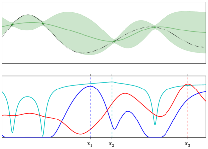
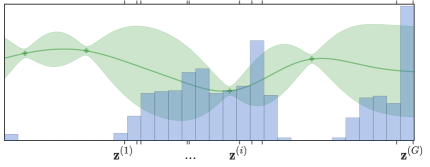
Figure 1: Visualization of Bayesian optimization with acquisition function portfolios. Top panel: visualization of the marginal GP posterior as well as the true objective function (dotted). Middle panel: plot of three acquisition functions in this portfolio, in this case EI (blue), PI (cyan), and TS (red). The purpose of Algorithm 2 is to select between these experts’ candidates $\mathbf{x}_{1}$, $\mathbf{x}_{2}$, and $\mathbf{x}_{3}$, respectively. Bottom panel: histogram of 1000 approximate samples from $p(\mathbf{x}_{\star}|\mathcal{D})$.

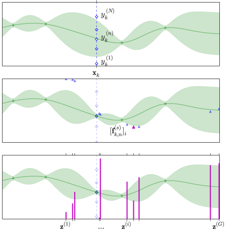
Figure 2: Visualization of the Entropy Search Portfolio. Top panel: for each candidate $\mathbf{x}_{k}$ (blue dashed line) we draw $N$ hallucinations $y_{k}^{(n)}$ (blue diamonds) from the predictive distribution. Middle panel: for each hallucination we augment the GP (green line and shaded area) and sample it $S$ times at the discrete points $\mathbf{z}^{(i)}$ to obtain the $\mathbf{f}_{kn}^{(s)}$ (blue triangles) for $s=1,\dots,S$. We find the minimizer of each vector $\mathbf{f}_{kn}^{(s)}$ (magenta triangle). Bottom panel: finally, we bin the $S$ minimizers into a discrete empirical distribution $\hat{p}$ depicted here as a magenta histogram.

3.1 Computing the ESP criterion

The utility function introduced in (4) can be approximated first by Monte Carlo integration, i.e.

$$u(\mathbf{x}_{k}|\mathcal{D})\approx\frac{1}{N}\sum_{n=1}^{N}H\big{[}\mathbf{x}_{\star}|\tilde{\mathcal{D}}_{k}^{(n)}\big{]}\;\text{for}\;y_{k}^{(n)} \sim p(y|\mathbf{x}_{k},\mathcal{D}),$$

where $\tilde{\mathcal{D}}_{k}^{(n)}=\mathcal{D}\cup\{(\mathbf{x}_{k},y_{k}^{(n)}\}$ is the hallucinated data. Note that this step only requires that we sample from our predictive distribution and in practice one can also use stratified or quasi-Monte Carlo to reduce the variance of this approximation. Next we must compute the entropy of the conditional distribution, given by $-\int p(\mathbf{x}_{\star}|\tilde{D})\log p(\mathbf{x}_{\star}|\tilde{\mathcal{D}})\,\mathrm{d}\mathbf{x}$. However, not only does this integral not have an analytic solution, but a simple Monte Carlo approximation is impractical because the quantity $\log p(\mathbf{x}_{\star}|\tilde{\mathcal{D}})$ is intractable to compute.

We will instead replace $p(\mathbf{x}_{\star}|\tilde{\mathcal{D}})$ with a discrete distribution $\hat{p}$ that is restricted to a particular discretization of the domain using a finite set of representer points. These points, denoted $\{\mathbf{z}^{(i)}\}_{i=1}^{G}$ will be sampled from some alternative measure as is done in (Hennig and Schuler, 2012). In order to obtain good performance it is desirable for the distribution of $\{\mathbf{z}^{(i)}\}$ to closely match the target distribution $p(\mathbf{x}_{\star}|\tilde{\mathcal{D}})$. Our proposed algorithm uses approximate samples from the distribution $p(\mathbf{x}_{\star}|\mathcal{D})$ which we expect to be closer to the target distribution than the functions EI or PI that were suggested previously. This step corresponds to Line 1 of Algorithm 2 after which the $\{\mathbf{z}^{(i)}\}$ are kept fixed for the remainder of the algorithm. In an effort to maintain the flow of this section, we defer the technical details of how these approximate samples are produced to Section 3.2.

Combining the Monte Carlo integration with this discretization, the utility for each recommendation can now be written as

$$u(\mathbf{x}_{k}|\mathcal{D})\approx\\ -\frac{1}{N}\sum_{n=1}^{N}\sum_{i=1}^{G}\hat{p}(\mathbf{x}_{\star}\!=\!\mathbf{z}^{(i)}|\tilde{\mathcal{D}}_{k}^{(n)})\log\hat{p}(\mathbf{x}_{\star}\!=\!\mathbf{z}^{(i)}|\tilde{\mathcal{D}}_{k}^{(n)}).$$

We are now left with the problem of computing the probability $\hat{p}(\mathbf{x}_{\star}=\mathbf{z}^{(i)}|\tilde{\mathcal{D}}_{k}^{(n)})$. Recall, however, that $\hat{p}$ is the distribution over minimizers of a GP-distributed function where the minimizers are restricted to a finite set. This can easily be sampled exactly. Let the random variable $[\mathbf{f}_{kn}]_{i}=f(\mathbf{z}^{(i)})$, $i=1,\ldots,G$, be a vector of latent function values evaluated at the representer points and conditioned on data $\tilde{\mathcal{D}}_{k}^{(n)}$. This vector simply has a Gaussian distribution and as a result we can produce $S$ samples $\mathbf{f}_{kn}^{(s)}\sim p(\cdot|\tilde{\mathcal{D}}_{k}^{(n)})$ from the resulting GP posterior. The probabilities necessary to compute the entropy can then be approximated by the relative counts

$$\hat{p}_{ikn}=\frac{1}{S}\sum_{s=1}^{S}\mathbb{I}\big{[}i=\operatorname*{arg\,min}_{j}[\mathbf{f}_{kn}^{(s)}]_{j}\big{]}$$ (6)

such that $\mathbf{z}^{(i)}$ is the minimizer among the sampled functions. Finally, by combining these ideas we can write our entropy-based meta-criterion as

$$u(\mathbf{x}_{k}|\mathcal{D})=-\frac{1}{N}\sum_{n=1}^{N}\sum_{i=1}^{G}\hat{p}_{ikn}\log\hat{p}_{ikn}.$$ (7)

Pseudocode computing this quantity is given in Algorithm 2 and we provide a corresponding visualization in Figure 2.

Algorithm 2 Entropy Search Portfolio (ESP)

0:  candidates $\{\mathbf{x}_{k}\}$, observations $\mathcal{D}$

1:  $\mathbf{z}^{(i)}\sim p(\mathbf{x}_{\star}|\mathcal{D}),\quad i=1,\dots,G$

2:  for $k=1:K$ do

3:     for $n=1:N$ do

4:        $y_{k}^{(n)}\sim p(y|\mathbf{x}_{k},\mathcal{D})$

5:        $\tilde{\mathcal{D}}_{k}^{(n)}=\mathcal{D}\cup\{(\mathbf{x}_{k},y_{k}^{(n)})\}$

6:        $\mathbf{f}_{kn}^{(s)}\sim p(\mathbf{f}|\tilde{\mathcal{D}}_{k}^{(n)})$ for $s=1:S$

7:        $\hat{p}_{ikn}=\frac{1}{S}\sum_{s}\mathbb{I}\big{[}i=\operatorname*{arg\,min}_{j}[\mathbf{f}_{kn}^{(s)}]_{j}\big{]}$

8:     end for

9:     $u_{k}=\frac{1}{N}\sum_{n=1}^{N}\sum_{i=1}^{G}\hat{p}_{ikn}\log\hat{p}_{ikn}$

10:  end for

11:  return  $\mathbf{x}_{k_{\star}}$ where $k_{\star}=\operatorname*{arg\,max}_{k}u_{k}$

3.2 Sampling posterior minimizers

The meta-criterion introduced in the previous section relied upon producing samples from (3), i.e. the posterior over global minima. While sampling from (3) is difficult in general, we can gain intuition by considering the finite domain setting. If the domain $\mathcal{X}$ is restricted to a finite set of $m$ points, the latent function $f$ takes the form of an $m$-dimensional vector $\mathbf{f}$. The probability that the $i$th element of $\mathbf{f}$ is optimal can then be written as $\int p(\mathbf{f}|\mathcal{D})\prod_{j\neq i}\mathbb{I}[f_{i}\leq f_{j}]\,d\mathbf{f}$. This suggests the following generative process: i) draw a sample from the posterior distribution $p(\mathbf{f}|\mathcal{D})$ and ii) return the index of the maximum element in the sampled vector. This process is known as Thompson sampling or probability matching when used as an arm-selection strategy in multi-armed bandits (Chapelle and Li, 2011). This same approach could be used for sampling the maximizer over a continuous domain $\mathcal{X}$. At first glance this would require constructing an infinite-dimensional object representing the function $f$. To avoid this, one could sequentially construct $f$ while it is being optimized. However, evaluating such an $f$ would ultimately have cost $\mathcal{O}(m^{3})$ where $m$ is the number of function evaluations necessary to find the optimum. Instead, we propose to sample and optimize an analytic approximation to $f$. We will briefly derive this approximation below.

Given a shift-invariant kernel $k$, a theorem of (Bochner, 1959) asserts the existence of its Fourier dual,

$$s(\mathbf{w})=\frac{1}{(2\pi)^{d}}\int e^{i\mathbf{w}^{\mathsf{T}}{\bm{\tau}}}k({\bm{\tau}},\mathbf{0})\,\mathrm{d}{\bm{\tau}},$$

i.e. the spectral density of $k$. Letting $p(\mathbf{w})=s(\mathbf{w})/\alpha$ be the associated normalized density, we can write the kernel as the expectation

$$k(\mathbf{x},\mathbf{x}^{\prime})=\alpha\,\mathbb{E}_{p(\mathbf{w})}[e^{-i\mathbf{w}^{\mathsf{T}}(\mathbf{x}-\mathbf{x}^{\prime})} ]$$ (8)

$$=2\alpha\,\mathbb{E}_{p(\mathbf{w},b)}[\cos(\mathbf{w}^{\mathsf{T}}\mathbf{x}+b) \cos(\mathbf{w}^{\mathsf{T}}\mathbf{x}^{\prime}+b)]\,,$$ (9)

where $b\sim\mathcal{U}[0,2\pi]$. Let ${\bm{\phi}}(\mathbf{x})=\sqrt{2\alpha/m}\cos(\mathbf{W}\mathbf{x}+\mathbf{b})$ denote an $m$-dimensional feature mapping and where $\mathbf{W}$ and $\mathbf{b}$ consist of $m$ stacked samples from $p(\mathbf{w},b)$. The kernel $k$ can then be approximated by the inner product of these features, $k(\mathbf{x},\mathbf{x}^{\prime})\approx{\bm{\phi}}(\mathbf{x})^{\mathsf{T}}{\bm{\phi}}(\mathbf{x}^{\prime})$. This approach was used by (Rahimi and Recht, 2007) as an approximation method in the context of kernel methods. The feature mapping ${\bm{\phi}}(\mathbf{x})$ allows us to approximate the Gaussian process prior for $f$ with a linear model $f(\mathbf{x})={\bm{\phi}}(\mathbf{x})^{\mathsf{T}}{\bm{\theta}}$ where ${\bm{\theta}}\sim\mathcal{N}(\mathbf{0},\mathbf{I})$ is a standard Gaussian. By conditioning on $\mathcal{D}$, the posterior for ${\bm{\theta}}$ is also multivariate Gaussian, ${\bm{\theta}}|\mathcal{D}\sim\mathcal{N}(\mathbf{A}^{-1}{\bm{\Phi}}^{\mathsf{T}}\mathbf{y},\sigma^{2}\mathbf{A}^{-1})$ where $\mathbf{A}={\bm{\Phi}}^{\mathsf{T}}{\bm{\Phi}}+\sigma^{2}\mathbf{I}$, $\mathbf{y}$ is the vector of the output data, and ${\bm{\Phi}}$ is a matrix of features evaluated on the input data.

Let ${\bm{\phi}}^{(i)}$ and ${\bm{\theta}}^{(i)}$ be a random set of features and the corresponding posterior weights sampled both according to the generative process given above. They can then be used to construct the function $f^{(i)}(\mathbf{x})={\bm{\phi}}^{(i)}(\mathbf{x})^{\mathsf{T}}{\bm{\theta}}^{(i)}$, which is an approximate posterior sample of $f$—albeit one with a finite parameterization. We can then maximize this function to obtain $\mathbf{z}^{(i)}=\operatorname*{arg\,min}_{\mathbf{x}\in\mathcal{X}}f^{(i)}(\mathbf{x})$, which is approximately distributed according to $p(\mathbf{x}_{\star}|\mathcal{D})$.

Finally, while this approach can be used to produce samples which implement the entropy meta-criterion of the previous section, it can also be used directly as an acquisition strategy. Consider the randomized strategy given by

$$\alpha_{\textsc{thompson}}(\mathcal{D})=\mathbf{x}_{\star}^{(0)}\quad\text{where}\quad\mathbf{x}_{\star}^{(0)}\sim p(\mathbf{x}_{\star}|\mathcal{D}).$$

Given the above description we can see that for finite $\mathcal{X}$ this is exactly the Thompson sampling algorithm. However, our derivation extends this approach to continuously varying functions. Finally we note that this technique was also used in a similar context by (Hernández-Lobato et al., 2014), albeit not directly as an acquisition function.

3.3 Additional details

In Algorithm 2 we summarize ESP, the meta-criterion developed in this work. The cost of this approach will be dominated by solving the linear system on line 6 of Algorithm 2. As a result the complexity will be on the order $\mathcal{O}(KNSt^{3})$, however this is only a constant-factor slowdown when compared to standard Bayesian optimization algorithms and can easily be parallelized.

One consideration we have not mentioned is the selection of hyperparameters, which can have a huge effect on the performance of any Bayesian optimization algorithm. For example, for kernels with lengthscale parameters chosen to be very small, then querying a point $\mathbf{x}$ will only allow the posterior to learn the model structure in a very small region around this point. If this parameter is chosen to be too small, this can greatly affect the optimization process as it will force the optimizer to uniformly explore small balls of width proportional to the lengthscale. For too large lengthscales, the model will be too smooth and similar difficulties arise.

Typical approaches to GP regression will often optimize the marginal likelihood as a means of setting these parameters. However, in the Bayesian optimization setting this approach is particularly ineffective due to the initial paucity of data. Even worse, such optimization can also lead to quite severe local maxima around the initial data points. In this work, we instead consider a fully Bayesian treatment of the hyperparameters. Let ${\bm{\psi}}$ denote a vector of hyperparameters which includes any kernel and likelihood parameters. Let $p({\bm{\psi}}|\mathcal{D})\propto p({\bm{\psi}})\,p(\mathcal{D}|{\bm{\psi}})$ denote the posterior distribution over these parameters where $p({\bm{\psi}})$ is a hyperprior and $p(\mathcal{D}|{\bm{\psi}})$ is the GP marginal likelihood. For a fully Bayesian treatment of ${\bm{\psi}}$ we must marginalize our acquisition strategy with respect to this posterior. The corresponding integral has no analytic expression and must be approximated using Monte Carlo.

Consider now drawing $M$ samples $\{{\bm{\psi}}^{(i)}\}$ from the posterior $p({\bm{\psi}}|\mathcal{D}_{t})$. Often an acquisition strategy is specified with respect to some internal acquisition function which is optimized at every iteration in order to select $\mathbf{x}_{t}$. These functions can then be approximately marginalized with respect to the hyperparameter samples in order to instead optimize an integrated acquisition function. This approach was taken in (Snoek et al., 2012) for the EI and PI acquisition functions. Note that the randomized Thompson sampling strategy, introduced in Section 3.2, only requires a single hyperparameter sample as we can see this as a joint sample from the hyperparameters and the function minimizer.

Our approach has additional complexity in that our candidate selection criterion depends on the hyperparameter samples as well. This occurs explicitly in lines (4–6) of Algorithm 2 which sample from the GP posterior. This can be solved simply by adding an additional loop over the hyperparameter samples. Our particular use of representer points in line 1 also depends on these hyperparameters. We can solve this problem by equally allocating our representers between the $M$ different hyperparameter samples.

4 Experiments

In this section, we evaluate the proposed method on several problems: two synthetic test functions commonly used for benchmarking in global optimization, two real-world datasets from the geostatistics community, and two simulated control problems. We compare ESP against two other portfolio methods, namely the Hedge portfolio of Hoffman et al. (2011) and RP, a random portfolio baseline which selects among its acquisition functions randomly.

All three portfolios consist of three commonly used base acquisition functions: EI, PI, and Thompson sampling. For EI we used the implementation available in the spearmint package, while the latter two were implemented in the same framework. All three methods were included in the portfolios. Note that we do not compare against GPUCB (Gaussian Process Upper Confidence Bounds) Srinivas et al. (2010) as the bounds do not apply directly when integrating over GP hyperparameters. This would require an additional derivation which we do not consider here.

The performance of the three constituent acquisition functions are provided in our figures for three reasons. First, the results show that indeed no single acquisition function is the top performer across all six objective functions that we optimized. Second, the purpose of the portfolio was to mitigate against a poor choice of acquisition function; therefore our target performance should be the best performing constituent. Surprisingly however, we find that, in two cases, the portfolio beat the top acquisition function. Recall that the portfolios do not know, a priori, which of their constituents will perform the best. Finally, this is also the first evaluation of Thompson sampling in continuous search spaces, although it was used for a separate purpose in the approximation method of Hernández-Lobato et al. (2014).

4.1 Model details and hyperparameter marginalization

For this set of experiments we use a Matérn kernel with smoothness parameter $\tfrac{5}{2}$. Note that this corresponds to a kernel of the form $k(\mathbf{x},\mathbf{x}^{\prime})=\nu^{2}\exp(-r)(1+r+\tfrac{1}{3}r^{2})$ where $r=\sqrt{5}(\mathbf{x}-\mathbf{x}^{\prime})^{\mathsf{T}}\mathup{diag}({\bm{\ell}}^{2})^{-1}(\mathbf{x}-\mathbf{x}^{\prime})$. Further, for the purposes of sampling the minimizer locations we need to sample from the spectral density of this kernel, which can be seen as a Student’s T distribution, $\mathcal{T}(0,\mathup{diag}({\bm{\ell}}^{2})^{-1},\tfrac{5}{2})$.

As noted in Section 3.3, rather than obtain maximum likelihood point estimates of the GP hyperparameters (i.e., kernel length-scale and amplitude, and prior constant mean), we marginalize them using 10 Markov chain Monte Carlo (MCMC) samples after each observation. Both improvement-based methods, EI and PI, can simply be evaluated with each sample and averaged. Meanwhile, in keeping with the Thompson strategy, our Thompson implementation only uses a single sample, namely the last one of the MCMC chain. As reported above, our proposed ESP method splits its 500 representer points equally among the hyperparameter samples. In other words, for each of the 10 MCMC samples we draw 50 points. In addition, in order to estimate $u(\mathbf{x}_{k}|\mathcal{D})$, for each of 5 simulated $y_{k}^{(n)}$ and each GP hyperparameter, ESP draws 1000 samples from $p(\mathbf{x}_{\star}|\tilde{\mathcal{D}}_{k}^{(n)})$, and then computes and averages the entropy estimates.

In the following experiments we evaluate the performance of each algorithm as a function of the number of function evaluations. When the true optimum is known, as in the case of the Branin and Hartmann 3 experiments, we measure performance by the absolute error. For all other minimization experiments, performance is given by the minimum function value obtained up to that iteration. Each experiment was repeated 25 times with different random seeds. For each method, we plot the mean performance over the repetitions as well as a shaded area one standard error away from the mean.

4.2 Global optimization test functions

We begin with two synthetic functions commonly used for benchmarking global optimization methods: Branin and Hartmann 3 (Lizotte, 2008). They are two- and three-dimensional, respectively, and are both continuous, bounded, and multimodal. The experiments were run up to a final horizon of $T=100$. Figure 3 reports the observed performance measured in absolute error on a logarithmic scale.

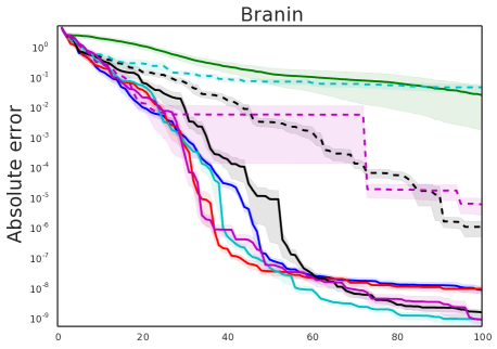
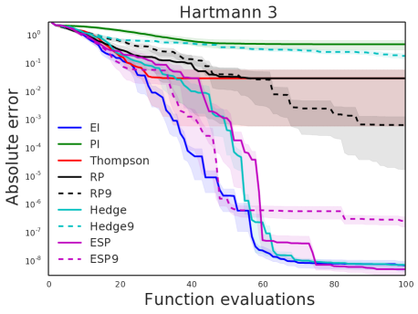
Figure 3: Absolute error of the best observation for the Branin and Hartmann 3 synthetic functions. The 9 additional random experts in RP9, GPHedge9, and ESP9 affect the RP and GPHedge methods much more dramatically than ESP on Hartmann 3. On Branin, a single outlier run out of 25 is negatively affecting the averaged results. When this run is masked, ESP9 achieves $<10^{-4}$ error by evaluation 40.

It is interesting to note that despite the poor performance of PI in this task, all portfolios still eventually outperform the base strategies. As expected, ESP makes the best use of its base experts and outperforms all other methods in both examples. In addition, note that each of the two domains have their own champion, EI being a clear winner on Hartmann 3, and Thompson being the more attractive option on Branin. This observation motivates the use of portfolios of acquisition functions.

In these synthetic experiments, we also demonstrate the robustness of ESP with respect to the inclusion of poor base strategies. We do so by adding 9 random experts to each portfolio (we denote these ESP9, RP9, etc.). These so-called random experts select a point uniformly at random in the bounding box $\mathcal{X}$. We expect this sort of random search to be comparable to the other base methods in the initial stage of the optimization and eventually provide too much exploration and not enough exploitation. Note that a few random experts in a portfolio could actually be beneficial in providing a constant source of purely exploratory candidates; precisely how many, however, is an interesting question we do not discuss in the present work. Nevertheless, for the dimensionality and difficulty of these examples, we propose 9 additional random experts as being too many and indeed we observe empirically that they substantially deteriorate performance for all portfolios.

In particular, we see that, especially on Hartmann 3, ESP is virtually unaffected until it reaches 6 digits of accuracy. Meanwhile, the progress made by RP is hindered by the random experts which it selects as frequently as the legitimate acquisition functions. Significantly worse is the performance of GPHedge which, due to the initial success of the random experts, favours these until the horizon is reached. Note in contrast that ESP does not rely on any expert’s past performance, which makes it robust to lucky guesses and time-varying expert performances. GPHedge could possibly be improved by tuning the reward function it uses internally but this is a difficult and problem dependent task. On Branin, a single outlier run is deteriorating the performance of ESP9. When masked, the mean performance achieves $10^{-4}$ by evaluation 40.

4.3 Geostatistics datasets

The next set of experiments were carried out on two datasets from the geostatistics community, referred to here as Brenda and Agromet (Clark and Harper, 2008). Since these datasets consist in finite sets of points, we transformed each of them into a function that we can query at arbitrary points via nearest neighbour interpolation. This produces a jagged piecewise constant function, which is outside the smoothness class of our surrogate models and hence a relatively difficult problem.

Brenda is a dataset of 1,856 observations in the depths of a copper mine in British Columbia, Canada, that was closed in 1990. The search domain is therefore three-dimensional and the objective function represents the quantity of underground copper. Agromet is a dataset of 18,188 observations taken in Natal Highlands, South Africa, where gold grade of the soil is the objective. The search domain here is two-dimensional.

We note that PI, which has so far been an under-achiever, outperforms EI on Agromet. This is further motivation for the use of portfolios, because our experience on the two synthetic experiments would have suggested that PI is a poor strategy. On both geological examples, RP is out-performed by GPHedge and ESP. We observe that ESP performs particularly well on Brenda, and on Agromet ESP is first, albeit by a very small margin. Recall that our original intention in using portfolios was to guard against choosing a poor acquisition function; however, on these examples ESP even outperforms the best of its constituent strategies (Thompson sampling in these two examples). This suggests that in addition to improving robustness to poor acquisition functions, portfolios could be used to boost overall performance.

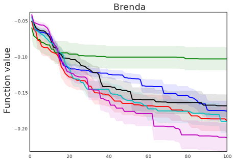
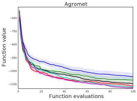
Figure 4: Best observed evaluation on mining datasets Brenda and Agromet. ESP outperforms the other portfolio methods while RP is dominated by all others.

4.4 Control tasks

Our final experiments compare the portfolio methods on two control tasks. Walker is an eight-dimensional control problem where the inputs are fed into a simulator which returns the walking speed of a bipedal robot (Westervelt and Grizzle, 2007). The code for the simulator is available online. This example was also used in a Bayesian optimization context by (Hernández-Lobato et al., 2014). Repeller is a nine-dimensional control problem considered in previous work on Bayesian optimisation portfolios (Hoffman et al., 2011, 2009). This problem simulates a particle in a two-dimensional world being dropped from a fixed starting region while accelerated downward by gravity. The task is to direct the falling particle through circular regions of low loss by placing 3 repellers with 3 degrees of freedom each, namely their position in the plane and repulsion strength. Figure 5 reports our results on both control tasks.

On these tasks, GPHedge performed poorly, while RP performs well. Meanwhile, ESP is the clear top performing portfolio method on Walker and competitive, if not tied, with RP on Repeller. We have also added the RP9, GPHedge9, and ESP9 methods in this experiment to once again demonstrate the robustness of ESP relative to its competitors. Indeed, both RP9 and GPHedge9 exhibit noticeably poorer performance than RP and GPHedge, while in contrast ESP9 is not significantly affected.

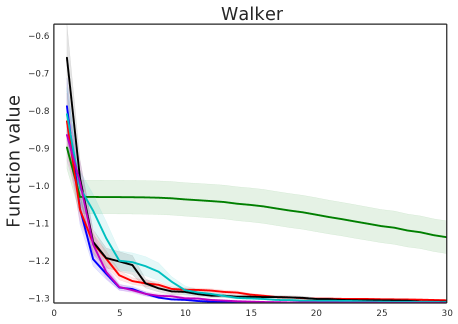
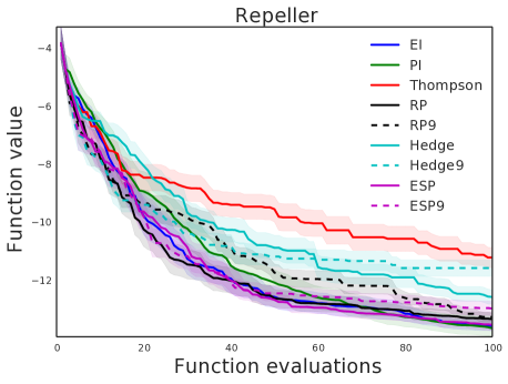
Figure 5: Best observed evaluation on the Walker and Repeller control tasks. Here we see ESP outperforming the other methods on Walker. On Repeller, ESP is once again competitive with the best methods and exhibits much more robustness to poor experts as evidenced by ESP9 following the performance of ESP so closely.

5 Conclusion

In this work we revisited the use of portfolios for Bayesian optimization. We introduced a novel, information-theoretic meta-criterion ESP which can indeed provide performance matching or even exceeding that of its component experts. This is particularly important since we show in our experiments that the best acquisition function varies between problem instances and is a priori unknown. We have also shown that ESP has robust behavior across functions of different dimensionality even when the members of its portfolio do not exhibit this behavior. Furthermore, ESP is more robust to poorly performing experts than other portfolio mechanisms.

Finally, we provided a mechanism for sampling representer points as a way of approximating $p(\mathbf{x}_{\star}|\mathcal{D})$ which is more principled than previous approaches which relied on slice sampling from surrogate measures. We additionally showed that this sampling mechanism can itself be used as an acquisition strategy, thereby extending the popular Thompson sampling approach to continuous spaces; we include the first empirical evaluation of this method within our results.

References

- Azimi et al. [2012] J. Azimi, A. Jalali, and X. Fern. Hybrid batch bayesian optimization. In ICML, 2012.
- Bergstra et al. [2011] J. Bergstra, R. Bardenet, Y. Bengio, and B. Kégl. Algorithms for hyper-parameter optimization. In Advances in Neural Information Processing Systems, pages 2546–2554, 2011.
- Bochner [1959] S. Bochner. Lectures on Fourier integrals. Princeton University Press, 1959.
- Brochu et al. [2009] E. Brochu, V. M. Cora, and N. de Freitas. A tutorial on Bayesian optimization of expensive cost functions, with application to active user modeling and hierarchical reinforcement learning. Technical Report UBC TR-2009-23 and arXiv:1012.2599v1, Dept. of Computer Science, University of British Columbia, 2009.
- Brochu et al. [2010] E. Brochu, T. Brochu, and N. de Freitas. A Bayesian interactive optimization approach to procedural animation design. In Proceedings of the 2010 ACM SIGGRAPH/Eurographics Symposium on Computer Animation, pages 103–112, 2010.
- Chapelle and Li [2011] O. Chapelle and L. Li. An empirical evaluation of Thompson sampling. In Advances in Neural Information Processing Systems, pages 2249–2257, 2011.
- Clark and Harper [2008] I. Clark and W. V. Harper. Practical Geostatistics 2000: Case Studies. Ecosse North America, 2008.
- de Freitas et al. [2012] N. de Freitas, A. Smola, and M. Zoghi. Exponential regret bounds for Gaussian process bandits with deterministic observations. In International Conference on Machine Learning, 2012.
- Freund and Schapire [1997] Y. Freund and R. E. Schapire. A decision-theoretic generalization of on-line learning and an application to boosting. Journal of computer and system sciences, 55(1):119–139, 1997.
- Garnett et al. [2010] R. Garnett, M. A. Osborne, and S. J. Roberts. Bayesian optimization for sensor set selection. In ACM/IEEE International Conference on Information Processing in Sensor Networks, pages 209–219. ACM, 2010.
- Hennig and Schuler [2012] P. Hennig and C. Schuler. Entropy search for information-efficient global optimization. The Journal of Machine Learning Research, 98888:1809–1837, 2012.
- Hernández-Lobato et al. [2014] J. M. Hernández-Lobato, M. W. Hoffman, and Z. Ghahramani. Predictive entropy search for efficient global optimization of black-box functions. In Advances in Neural Information Processing Systems, 2014.
- Hoffman et al. [2014] M. Hoffman, B. Shahriari, and N. de Freitas. On correlation and budget constraints in model-based bandit optimization with application to automatic machine learning. In AI and Statistics, pages 365–374, 2014.
- Hoffman et al. [2009] M. W. Hoffman, H. Kueck, N. de Freitas, and A. Doucet. New inference strategies for solving Markov decision processes using reversible jump MCMC. In Uncertainty in Artificial Intelligence, pages 223–231, 2009.
- Hoffman et al. [2011] M. W. Hoffman, E. Brochu, and N. de Freitas. Portfolio allocation for Bayesian optimization. In Uncertainty in Artificial Intelligence, pages 327–336, 2011.
- Hutter et al. [2011] F. Hutter, H. H. Hoos, and K. Leyton-Brown. Sequential model-based optimization for general algorithm configuration. In LION, pages 507–523, 2011.
- Jones [2001] D. Jones. A taxonomy of global optimization methods based on response surfaces. J. of Global Optimization, 21(4):345–383, 2001.
- Jones et al. [1998] D. Jones, M. Schonlau, and W. Welch. Efficient global optimization of expensive black-box functions. J. of Global optimization, 13(4):455–492, 1998.
- Lizotte [2008] D. Lizotte. Practical Bayesian Optimization. PhD thesis, University of Alberta, Canada, 2008.
- Lizotte et al. [2007] D. Lizotte, T. Wang, M. Bowling, and D. Schuurmans. Automatic gait optimization with Gaussian process regression. In Proc. of IJCAI, pages 944–949, 2007.
- Marchant and Ramos [2012] R. Marchant and F. Ramos. Bayesian optimisation for intelligent environmental monitoring. In NIPS workshop on Bayesian Optimization and Decision Making, 2012.
- Martinez-Cantin et al. [2007] R. Martinez-Cantin, N. de Freitas, A. Doucet, and J. A. Castellanos. Active policy learning for robot planning and exploration under uncertainty. Robotics Science and Systems, 2007.
- Močkus et al. [1978] J. Močkus, V. Tiesis, and A. Žilinskas. The application of bayesian methods for seeking the extremum. In L. Dixon and G. Szego, editors, Toward Global Optimization, volume 2. Elsevier, 1978.
- Osborne [2010] M. Osborne. Bayesian Gaussian Processes for Sequential Prediction, Optimization and Quadrature. PhD thesis, University of Oxford, 2010.
- Rahimi and Recht [2007] A. Rahimi and B. Recht. Random features for large-scale kernel machines. In Advances in Neural Information Processing Systems, pages 1177–1184, 2007.
- Rasmussen and Williams [2006] C. E. Rasmussen and C. K. I. Williams. Gaussian Processes for Machine Learning. The MIT Press, 2006.
- Snoek et al. [2012] J. Snoek, H. Larochelle, and R. P. Adams. Practical Bayesian optimization of machine learning algorithms. In Advances in Neural Information Processing Systems, pages 2951–2959, 2012.
- Srinivas et al. [2010] N. Srinivas, A. Krause, S. M. Kakade, and M. Seeger. Gaussian process optimization in the bandit setting: No regret and experimental design. In International Conference on Machine Learning, pages 1015–1022, 2010.
- Swersky et al. [2013] K. Swersky, J. Snoek, and R. P. Adams. Multi-task Bayesian optimization. In Advances in Neural Information Processing Systems, pages 2004–2012, 2013.
- Thornton et al. [2013] C. Thornton, F. Hutter, H. H. Hoos, and K. Leyton-Brown. Auto-WEKA: Combined selection and hyperparameter optimization of classification algorithms. In Knowledge Discovery and Data Mining, pages 847–855, 2013.
- Villemonteix et al. [2009] J. Villemonteix, E. Vazquez, and E. Walter. An informational approach to the global optimization of expensive-to-evaluate functions. J. of Global Optimization, 44(4):509–534, 2009.
- Wang et al. [2013] Z. Wang, S. Mohamed, and N. de Freitas. Adaptive Hamiltonian and Riemann manifold Monte Carlo samplers. In International Conference on Machine Learning, pages 1462–1470, 2013.
- Wang et al. [2014] Z. Wang, B. Shakibi, L. Jin, and N. de Freitas. Bayesian multi-scale optimistic optimization. In AI and Statistics, pages 1005–1014, 2014.
- Westervelt and Grizzle [2007] E. Westervelt and J. Grizzle. Feedback Control of Dynamic Bipedal Robot Locomotion. Control and Automation Series. CRC PressINC, 2007. ISBN 9781420053722.