Full Halo Coronal Mass Ejections: Arrival at the Earth
Abstract
A geomagnetic storm is mainly caused by a front-side coronal mass ejection (CME) hitting the Earth and then interacting with the magnetosphere. However, not all front-side CMEs can hit the Earth. Thus, which CMEs hit the Earth and when they do so are important issues in the study and forecasting of space weather. In our previous work (Shen et al., 2013), the de-projected parameters of the full-halo coronal mass ejections (FHCMEs) that occurred from 2007 March 1 to 2012 May 31 were estimated, and there are 39 front-side events could be fitted by the GCS model. In this work, we continue to study whether and when these front-side FHCMEs (FFHCMEs) hit the Earth. It is found that 59% of these FFHCMEs hit the Earth, and for central events, whose deviation angles , which are the angles between the propagation direction and the Sun-Earth line, are smaller than 45 degrees, the fraction increases to 75%. After checking the deprojected angular widths of the CMEs, we found that all of the Earth-encountered CMEs satisfy a simple criterion that the angular width () is larger than twice the deviation angle (). This result suggests that some simple criteria can be used to forecast whether a CME could hit the Earth. Furthermore, for Earth-encountered CMEs, the transit time is found to be roughly anti-correlated with the de-projected velocity, but some events significantly deviate from the linearity. For CMEs with similar velocities, the differences of their transit times can be up to several days. Such deviation is further demonstrated to be mainly caused by the CME geometry and propagation direction, which are essential in the forecasting of CME arrival.
1 Introduction
The halo coronal mass ejections (CMEs), which appear to surround the occulting disk of coronagraphs, are preliminarily supposed to be propagating along the Sun-Earth line(Howard et al., 1982). Under this assumption, the front-side halo CMEs might be good candidates for Earth-impacted CMEs; however, not all of the front-side halo CMEs can hit the Earth. The ratio of the front-side halo CMEs hitting the Earth varied from 65% to 80%, which has been reported in different literature reports(Yermolaev and Yermolaev, 2006, and reference therein). In addition, most works are concerned about the geoeffectiveness of halo CMEs(e.g. Webb, 2002; Wang et al., 2002; Zhao and Webb, 2003; Zhang et al., 2007; Gopalswamy et al., 2007). The ratio of the front-side halo CMEs with geoeffectiveness varied from 45% to 71%. All of these works suggested that not all front-side halo CMEs can hit the Earth. Thus, what type of front-side halo CMEs can hit the Earth has been discussed by many authors(e.g. Wang et al., 2002; Zhang et al., 2003; Kim et al., 2005; Moon et al., 2005). Before the launch of the Solar Terrestrial Relations Observatory (STEREO), only coronagraph images and in situ measurements could be used to observe the CMEs near the Sun and the interplanetary CMEs (ICME) near the Earth respectively. Thus, direct connections between the CMEs near the Sun and the ICMEs near 1 AU might be unclear, especially during the solar maximum. Recently, using the large field of view observations from the Heliospheric imagers in the Sun-Earth-Connection Coronal and Heliospheric Investigation (SECCHI) (Howard et al., 2008) onboard STEREO, the propagation of CMEs could be well tracked continuously from the Sun to 1 AU. In this manner, the ejecta observed near the Earth and the CMEs that occurred near the Sun can be related in a more precise way. Can we re-investigate how many and what type of front-side halo CMEs can hit the Earth? In addition, we note that the apparent angular width threshold used to define the halo CMEs in previous works varied greatly, such as 120∘, 130∘, 140∘ and 360∘. If we apply the apparent angular width = 360∘ only, will the ratio and the criteria of the front-side full halo CMEs arriving at the Earth be changed?
In addition, if a CME can hit the Earth, its arrival time becomes an important issue in space weather forecasting. Recently, various kinematics and magnetohydrodynamic (MHD) models have been developed to forecast the arrival time of CMEs(e.g. Fry et al., 2003; Odstrcil et al., 2004; Tóth et al., 2005; Mckenna-Lawlor et al., 2006; Feng and Zhao, 2006; Shen et al., 2007; Feng et al., 2007; Shen et al., 2010; Feng et al., 2010, and reference therein) In those models, the velocity, propagation direction and angular width of the CMEs are used as the initial parameters. However, the following basic questions are still not fully answered. What are the key parameters that determine the transit time of the CMEs from the Sun to the Earth? What is the extent of influence of the leading parameter? The CME’s initial speed has been correlated with the transit time of the CME from the Sun to 1 AU(Cane et al., 2000; Wang et al., 2002; Zhang et al., 2003; Schwenn et al., 2005; Shanmugaraju and Vršnak, 2014). Some simple equations were established to calculate the possible arrival time of the CMEs based on their initial velocities. However, the deviation between the calculated transit times and the observations is large. One possible reason for this deviation is that the CME’s velocity might change greatly during its propagation in the interplanetary space due to the influence of the background solar wind(e.g. Gopalswamy et al., 2000). Using a constant acceleration (or deceleration) assumption, Gopalswamy et al. (2001, 2005) developed an empirical CME arrival (ECA) model to predict the arrival time of Earth-directed CMEs. However, the acceleration (or deceleration) may also be changed during the propagation of CMEs in the interplanetary space. Recently, some other CME propagation time forecasting models were developed based on aerodynamic drag models(e.g. Vršnak et al., 2013). The aerodynamic drag models assume that the acceleration (or deceleration) of CMEs depends on the velocity difference between the CME and the background solar wind. Most of the above works are mainly focused on the velocity of the CME. Are there any other parameters that would exert significant influence on the propagation time of CMEs from the Sun to the Earth? How significant the influence of these parameters? The propagation direction of CMEs might be another important parameter. It has been taken into account in many CME arrival time forecasting models, such as the advanced version of the drag-based model (DBM, http://oh.geof.unizg.hr/DBM/dbm.php), the ENLIL model and other MHD models(e. g. Odstrcil, 2003). Recently, based on a self-similar expansion assumption and a theoretical computation(Davies et al., 2012), Möstl and Davies (2012) suggested that the propagation time of a CME is influenced by its propagation direction and the angular width.
In our previous work (Shen et al. (2013), referred to as Paper I hereafter), the projection effect of full-halo CMEs (FHCMEs) listed in the CDAW CME catalog(Yashiro et al., 2004) with an apparent angular width of 360∘ occurred from 2007 March 1 to 2012 May 31 was studied. In Paper I, the Graduated Cylindrical Shell (GCS) model (Thernisien et al., 2006, 2009; Thernisien, 2011) was applied on the STEREO/COR2 and SOHO observations to obtain the de-projected kinematic parameters of these FHCMEs. Among the total of 88 events studied in paper I, 48 events originated from the front of the solar disk. Table 1 in this paper and Table B in our online list (http://space.ustc.edu.cn/dreams/fhcmes/) present the parameters of these front-side full halo CMEs (FFHCMEs). Of the total of 48 FFHCMEs, there are nine events that could not be fitted by the GCS model. The remaining 39 events with well-established de-projected parameters will be studied in detail here. In this work, we will verify whether these FFHCMEs hit the Earth by using the continuous CME propagation observations of COR2, HI1, HI2 on board the STEREO spacecraft and the in situ measurements of the WIND and ACE satellites. Next, we attempt to answer the main questions of which and when the FFHCMEs will hit the Earth based on the de-projected parameters. In section 2, we introduce the method to determine the interplanetary counterpart for a given FFHCME. Based on the list of the FFHCMEs and their associated interplanetary counterparts, the type of the Earth-encountered FFHCMEs will be discussed in section 3. In section 4, the parameters that affect the transit time of CMEs from the Sun to the Earth will be discussed. A conclusion and some discussions of the results will be provided in the last section.
2 Methods
| No | CME date | Direction | begin | end | ||||
| 1 | 2009/12/16 04:30:03 | E07,N09 | 11 | 45 | 411 | — | 2009/12/19 09:49 | 2009/12/20 09:22 |
| 2 | 2010/02/07 03:54:03 | E06,S07 | 9 | 81 | 481 | 2010/02/11 00:00 | 2010/02/11 13:00 | 2010/02/11 22:00 |
| 3 | 2010/02/12 13:42:04 | E01,N11 | 11 | 84 | 550 | 2010/02/15 17:40 | 2010/02/16 04:00 | 2010/02/16 12:00 |
| 4 | 2010/04/03 10:33:58 | E01,S27 | 27 | 84 | 853 | 2010/04/05 07:56 | 2010/04/05 12:00 | 2010/04/06 16:00 |
| 5 | 2010/05/23 18:06:05 | W16,N07 | 17 | 70 | 365 | 2010/05/28 01:58 | 2010/05/28 19:00 | 2010/05/29 17:00 |
| 6 | 2010/05/24 14:06:05 | W26,S06 | 26 | 63 | 552 | — | — | — |
| 7 | 2010/08/01 13:42:05 | E38,N20 | 42 | 93 | 1262 | 2010/08/03 17:00 | 2010/08/04 10:00 | 2010/08/05 02:00 |
| 8 | 2010/08/07 18:36:06 | E36,S06 | 36 | 83 | 779 | — | 2010/08/11 05:00 | 2010/08/12 17:00 |
| 9 | 2010/08/14 10:12:05 | W42,S11 | 43 | 119 | 864 | — | — | — |
| 10 | 2010/12/14 15:36:05 | W35,N39 | 50 | 112 | 856 | — | — | — |
| 11 | 2011/02/14 18:24:05 | W08,N01 | 8 | 61 | 365 | — | 2011/02/18 10:30 | 2011/02/18 19:30 |
| 12 | 2011/02/15 02:24:05 | W05,S07 | 8 | 140 | 764 | 2011/02/18 01:00 | 2011/02/18 20:00 | 2011/02/20 08:00 |
| 13 | 2011/03/07 20:00:05 | W34,N33 | 45 | 104 | 1933 | — | — | — |
| 14 | 2011/06/02 08:12:06 | E30,S03 | 30 | 92 | 961 | 2011/06/04 20:00 | 2011/06/05 02:00 | 2011/06/05 18:00 |
| 15 | 2011/06/07 06:49:12 | — | — | — | —- | — | — | — |
| 16 | 2011/06/21 03:16:10 | E20,N07 | 21 | 93 | 964 | 2011/06/23 02:00 | 2011/06/23 06:00 | 2011/06/24 06:00 |
| 17 | 2011/08/03 14:00:07 | W10,N12 | 15 | 124 | 925 | 2011/08/04 21:15 | 2011/08/05 03:30 | 2011/08/05 17:30 |
| 18 | 2011/08/04 04:12:05 | W36,N24 | 42 | 107 | —- | 2011/08/05 17:30 | 2011/08/06 22:00 | 2011/08/07 22:00 |
| 19 | 2011/08/09 08:12:06 | W45,N16 | 47 | 133 | 1594 | — | — | — |
| 20 | 2011/09/06 02:24:05 | — | — | — | —- | — | 2011/09/08 10:00 | 2011/09/09 12:00 |
| 21 | 2011/09/06 23:05:57 | W41,N19 | 44 | 116 | 901 | 2011/09/09 12:00 | 2011/09/10 03:00 | 2011/09/10 15:00 |
| 22 | 2011/09/22 10:48:06 | E72,N06 | 72 | 131 | 1823 | — | — | — |
| 23 | 2011/09/24 12:48:07 | E47,N06 | 47 | 119 | 1768 | 2011/09/26 12:00 | 2011/09/26 20:00 | 2011/09/28 00:00 |
| 24 | 2011/09/24 19:36:06 | — | — | — | —- | — | — | — |
| 25 | 2011/10/22 01:25:53 | — | — | — | —- | — | — | — |
| 26 | 2011/10/22 10:24:05 | — | — | — | —- | 2011/10/24 17:38 | 2011/10/25 00:00 | 2011/10/25 16:00 |
| 27 | 2011/10/27 12:00:06 | E42,N26 | 48 | 51 | —- | — | — | — |
| 28 | 2011/11/09 13:36:05 | E36,N24 | 42 | 172 | 1074 | 2011/11/12 05:26 | 2011/11/12 14:51 | 2011/11/13 11:09 |
| 29 | 2011/11/26 07:12:06 | W35,N17 | 38 | 177 | 900 | 2011/11/28 20:51 | 2011/11/29 00:12 | 2011/11/29 04:53 |
| 30 | 2012/01/02 15:12:40 | — | — | — | —- | 2012/01/05 15:50 | 2012/01/04 00:00 | 2012/01/06 02:43 |
| 31 | 2012/01/16 03:12:10 | E57,N39 | 64 | 124 | 958 | — | — | — |
| 32 | 2012/01/19 14:36:05 | E17,N43 | 45 | 141 | 1090 | 2012/01/22 05:10 | 2012/01/23 00:13 | 2012/01/24 15:09 |
| 33 | 2012/01/23 04:00:05 | W16,N41 | 43 | 193 | 1906 | 2012/01/24 14:30 | — | — |
| 34 | 2012/01/26 04:36:05 | W71,N56 | 79 | 85 | 1033 | — | — | — |
| 35 | 2012/01/27 18:27:52 | W78,N27 | 79 | 179 | 1807 | 2012/01/30 15:56 | — | — |
| 36 | 2012/02/09 21:17:36 | E42,N29 | 49 | 79 | 648 | — | — | — |
| 37 | 2012/02/10 20:00:05 | E25,N20 | 31 | 74 | 583 | — | 2012/02/14 17:58 | 2012/02/16 05:33 |
| 38 | 2012/02/23 08:12:06 | W61,N28 | 64 | 135 | 442 | 2012/02/26 20:58 | 2012/02/27 17:53 | 2012/02/28 15:40 |
| 39 | 2012/03/04 11:00:07 | E41,N27 | 47 | 150 | 1190 | — | — | — |
| 40 | 2012/03/05 04:00:05 | — | — | — | —- | 2012/03/07 03:28 | 2012/03/07 20:50 | 2012/03/08 11:41 |
| 41 | 2012/03/07 00:24:06 | E36,N33 | 47 | 140 | 2012 | 2012/03/08 10:54 | 2012/03/09 05:19 | 2012/03/11 08:03 |
| 42 | 2012/03/09 04:26:09 | W01,N06 | 6 | 73 | 1188 | — | — | — |
| 43 | 2012/03/10 18:12:06 | W16,N18 | 23 | 107 | 1271 | 2012/03/12 08:17 | 2012/03/12 21:41 | 2012/03/15 08:42 |
| 44 | 2012/03/13 17:36:05 | W37,N33 | 47 | 104 | 1525 | 2012/03/15 12:05 | 2012/03/16 00:51 | 2012/03/16 12:09 |
| 45 | 2012/04/05 21:25:07 | — | — | — | —- | — | — | — |
| 46 | 2012/04/09 12:36:07 | W40,N12 | 41 | 94 | 892 | — | — | — |
| 47 | 2012/05/12 00:00:05 | E25,S10 | 26 | 65 | 939 | — | — | — |
| 48 | 2012/05/17 01:48:05 | — | — | — | —- | — | — | — |
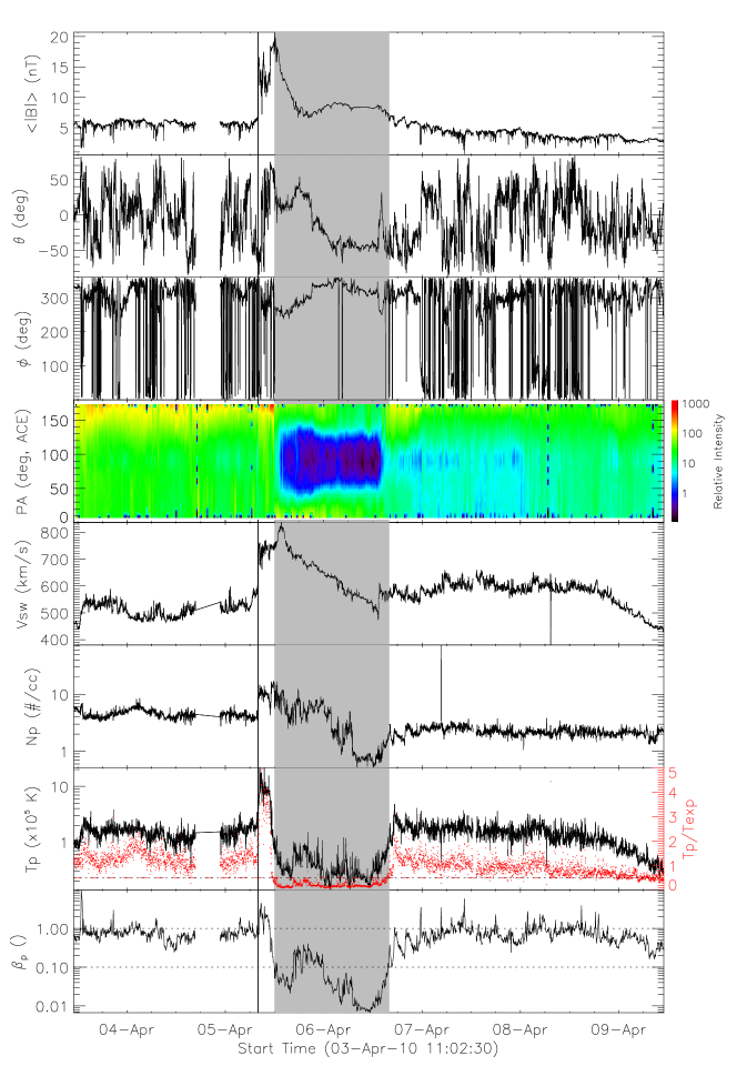
The interplanetary magnetic field and the solar wind plasma observations from WIND and ACE satellites are used to examine whether an interplanetary CME (ICME) was recorded near the Earth the six days following the launch of the CME with an Earthward potential. Previous works used different criteria to identify the ICME(e. g. Wang et al., 2002, 2004; Jian et al., 2006, and reference there in). In this paper, the following characteristics are used in the investigation: (1) enhanced magnetic field intensity, (2) smoothly changing field direction, (3) relatively low proton temperature, (4) low proton plasma beta, and (5) bidirectional streaming of electrons. An ICME structure is recognized when it fits at least three of the criteria listed above. The detailed observations of the identified ICME are provided in our online website (http://space.ustc.edu.cn/dreams/fhcmes/). Figure 1 shows the in situ observations from 2010 April 3 11:00UT to 2010 April 9 11:00UT, in the next six days after the launch of the CME occurred at 2010 April 3 10:33:58UT. For this event, an obvious ICME was recorded from 2010 April 5 12:00UT to 2010 April 6 16:00UT by WIND and ACE, which is indicated by the gray region in the Figure 1. This ICME is treated as the possible interplanetary counterpart of the 2010 April 3 10:33:58UT CME. In addition, a shock ahead of this ICME impacted the Earth at approximately 2010 April 5 08:00UT.
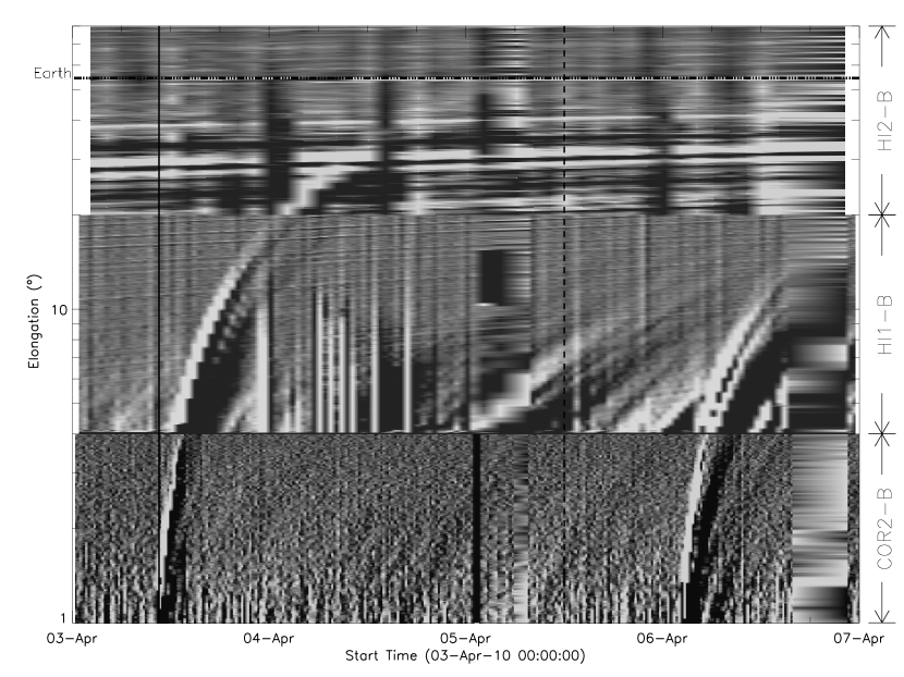
If there is at least one ICME recorded in the next six days after a CME was launched, the Time-Elongation Angle maps (J-maps) (e. g. Sheeley et al., 1999; Davis et al., 2009) are used to perform further verification of the association between the ICMEs recorded near the Earth and the FFHCMEs near the Sun. A 64-pixel-wide slice is placed along the ecliptical plane in the running-difference images from COR2, HI1 and HI2 on board STEREO, and the slices adopted at different times are stacked to obtain the J-map. A 64-pixel corresponds to 0.95 solar radius for COR2 and 1.25∘ and 4.38∘ of the elonagtion angle in the HI1 and HI2 field of view respectively. Figure 2 shows the J-map for the 2010 April 3 10:33:58UT CME. As seen in Figure 2, after the CME take-off (the vertical solid line), a black-white track that corresponds to the front of this CME extended to the region with an elongation angle of 60∘. At the time that the ICME was observed at 1 AU (indicated by the vertical dashed line), the front of this CME also reached a location near the Earth (shown by the horizontal dashed-dotted line). Thus, the ICME observed near the Earth from 2010 April 5 12:00UT to 2010 April 6 16:00UT was well associated with the 2010 April 3 10:33:58UT CME. In this manner, we found that a total of 27 of the 48 FFHCMEs considered hit the Earth. The 7th column of Table 1 shows the arrival time of the shock driven by the CME. The 8th and 9th columns present the beginning and ending times of the associated ICMEs. The ‘—’ symbol denotes that no ICME or shock was associated with this FFHCME.
3 Which CMEs arrived at the Earth?

Figure 3 shows the distribution of the propagation directions of all 39 FFHCMEs whose de-projected parameters were well established. It should be noted that, in the following analysis, only these 39 FFHCMEs were used. Those propagation directions were distributed in a large range, from E73∘ to W71∘ of longitude. According to their propagation longitudes, all 39 FFHCMEs can be classified into 20 eastern events and 19 western events. However, the propagation directions distribution in the north and south sides exhibit an obvious asymmetry. There are a total of 30 events propagating in the northern heliosphere and only nine events in the southern heliosphere. This asymmetry might be caused by the fact that the northern hemisphere is more active than the southern hemisphere in the ascending phase of the 24th solar cycle(e.g. Svalgaard and Kamide, 2013).
In the 39 events whose de-projected parameters have been obtained, 59% (23) of them hit the Earth. The solid dots in Figure 3 show the events that arrived at the Earth. The figure shows that their propagation longitudes are distributed in a range of [E47∘, W61∘], which is more narrow than the longitudinal distributions of all FFHCMEs. Note that the most eastern of the Earth-encountered events propagated at E47∘, and the most western event came from W61∘. This observation is consistent with the previous result that it is difficult for the east limb CMEs to hit the Earth(Wang et al., 2002; Zhang et al., 2003). In addition, the longitude range of most (21/23) of the Earth-encountered FFHCMEs is [E40∘,W40∘]. Meanwhile, for the FFHCMEs whose propagating longitudes located in this region, approximately 72% of them arrived at the Earth. This result suggests that the central events with propagation longitudes in the range of [E40∘, W40∘] are more likely to hit the Earth.
The deviation angle , which is defined as the angle between the propagation direction and the Sun-Earth line, is used to discriminate among the possible Earth-encountered CMEs. From Figure 4, 24 FFHCMEs propagated with and 75% (18) of them hit the Earth. Meanwhile, for the 13 FFHCMEs with , 77% (10) of them arrived at the Earth. For comparison, only one main body or the flux rope structure of five limb FFHCMEs with hit the Earth. It should be noted that, one shock driven by another limb CME hit the Earth. But, in this work, we mainly discussed whether the main body or the flux rope like structure of the CME hit the Earth. This observation confirms the previous result that the central CMEs can hit the Earth with higher possibility. In addition, five events with arrived at the Earth. Upon checking their de-projection parameters, we find that all of these events are wide events and that their minimum angular width is 103∘. This observation indicates that the limb CMEs can also impact the Earth if they are wide.

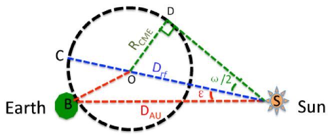
Simply by assuming that a CME moves as a self-similar expansion ball (e.g. Davies et al., 2012; Möstl and Davies, 2012) as shown in Figure 5, one can expect that the CME can hit the Earth when its angular width is larger than twice the deviation angle, i.e., . The dotted-dashed line in Figure 5 indicates . Based on the previous analysis, only CMEs located in the region above this line could hit the Earth. The observations that all of the Earth-encountered FFHCMEs are located in the upper region confirm the above conclusion. In addition, a large fraction (74%, 25/34) of FFHCMEs that fit the condition of hit the Earth. For comparison, all four events under the dotted-dashed line did not hit the Earth. This result indicates that the can be a useful criterion to forecast whether a CME would hit the Earth; therefore, the angular width is another important parameter in the space weather forecasting model.
Note that some CME events that were launched from regions close to the solar-disc center or fit the criterion of did not hit the Earth. One possible reason is that those CMEs may be deflected during their interaction with other CMEs(e.g. Xiong et al., 2009; Wang et al., 2011; Lugaz et al., 2012; Shen et al., 2012). Lugaz et al. (2012) studied the interaction between the CMEs occurred on 2010 May 23 and 2010 May 24, which are the No 5 and No 6 events, respectively, in our list. They found that the Earth-direct CME on 2010 May 24 had missed the Earth, which was a result of the interaction with the 2010 May 23 CME. In our investigation, six events with and did not hit the Earth. By carefully checking the heliospheric images from STEREO HI1 and HI2, we found that two events might be affected by their interaction with other CMEs: the 2012 May 24 event, which was studied by Lugaz et al. (2012), and the 2012 March 9 event. Why did the CMEs of the other four events not hit the Earth? A possible reason is that the CMEs might be deflected during their propagation in the corona (e.g. MacQueen et al., 1986; Gopalswamy and Thompson, 2000; Cremades and Bothmer, 2004; Kilpua et al., 2009; Gui et al., 2011; Shen et al., 2011; Zhou and Feng, 2013) as well as in the interplanetary space(e.g. Wang et al., 2004, 2006, 2013).
4 When did CMEs arrive at the Earth?

Figure 6 shows that the transit times of the CMEs from the Sun to 1 AU varied with the de-projection velocities of the CMEs. In Figure 6, the propagation time exhibits an anti-correlation with the de-projected velocities, but the dispersion is large. For the CMEs with similar velocities, the difference of the transit time can be up to tens of hours. For example, there are eight events whose velocities are 1000 (from 800 to 1200). The transit time of these events from the Sun to 1 AU varied from 37 hours for the 2011 August 3 event to 82 hours for the 2012 January 19 event. The difference between the propagation times is approximately 2 days.
Why do these CMEs with similar velocities have quite a different transit time from the Sun to 1 AU? It is probably because the CMEs have a circular-like front, and it is not always true that the leading front of a CME encounters the Earth. This effect means that in the case of ‘non-central’ impact, the CME forehead reaches a distance larger than 1 AU at the time when the CME arrival is recorded in the in situ observations near the Earth. A well-investigated case can be found in the most recent work by Wang et al. (2013), in which a CME occurred on 2008 September 13 passed through both the WIND and STEREO-B spacecraft at 1 AU. The arrival time of this CME at STEREO-B was approximately two days later than that at WIND. Again, we assume that the CME is a self-similar expansion ball radially propagating along the direction with a deviation angle of . When the observatory at 1 AU detected this CME, the real propagation distance of the CME tip along its propagation direction (, the length of SC in Figure 5) was obviously larger than 1 AU (). The difference between the and 1 AU, , depends on the angular width of the CME () and the propagation direction . The could be obtained by:
| (1) |
in which is the radius of this CME, which can be calculated from the equation of:
| (2) |
From Equations 1 and 2, the real propagation distance can be determined if the angular width and deviation angle are all known. To improve the comparison, we choose eight events with similar velocities in the range of for the further study. Figure 7 shows that calculated real propagation distance varied with the observed propagation time of these eight events based on the de-projected parameters obtained in paper I. Additionally, the of these events varied over a large range, from 1.04 AU to 1.53 AU. As shown in the previous analysis, could be treated as the real propagation distance of these CMEs along their propagation direction when they eventually arrived at 1 AU. As shown in Figure 7, the propagation time and the real propagating distance of these events have obvious positive correlation. This result indicates that the different transit time of CMEs with similar velocities might be caused primarily by the different part of the circular-like CME front arriving at 1 AU. From equations 1 and 2, the propagation distance of the CME tip is related to the angular width and the propagation direction. Thus, the true angular width and the propagation direction are all important parameters in the CME arrival time forecasting as well as the CME’s velocity and the background solar wind speed (e.g. Vršnak and Žic, 2007; Temmer et al., 2011).

The propagation of CMEs in the interplanetary space can be described by an aerodynamic drag model(e.g. Chen, 1996; Maloney and Gallagher, 2010; Vršnak et al., 2013; Lugaz and Kintner, 2012, and reference therein). Here, we use a simplified equation of the aerodynamic drag model from Maloney and Gallagher (2010) as:
| (3) |
in which C is a constant number. The dashed line in Figure 7 shows the result of the aerodynamic drag model by assuming the initiation speed of a CME is 1000, the solar wind speed is 450 . The value is obtained from a fitting process. In this figure, almost all of the points are close to the dashed line. Therefore, the propagation process of these CMEs could be well described by the aerodynamic drag model. Thus, the self-similar expansion model combined with the aerodynamic drag model might be a powerful tool to forecast the Earth arrival times of CMEs.
5 Conclusion and Discussion
In this work, we studied whether and when the front-side full halo CMEs that occurred from 2007 March 1 to 2012 May 31, hit the Earth. The de-projected parameters of those CMEs were obtained in our previous work(Shen et al., 2013). The in situ observations combined with the SECCHI/COR2 SECCHI/HI-1 and SECCHI/HI-2 observations from STEREO were used to verify whether these FFHCMEs hit the Earth. We conclude the following:
-
1.
Approximately 59% of the FFHCMEs studied in this work arrived at the Earth. The central CMEs, which propagated in the longitudinal range [E40∘, W40∘] or , can arrive at the Earth with higher probability.
-
2.
The FFHCMEs with an angular width of more than twice the deviation angle can hit the Earth. All of the Earth-encountered events fit the criterion , and 74% of the FFHCMEs events that fit the criterion of hit the Earth. Thus, the simple criterion () might be a useful tool to forecast whether a CME will hit the Earth.
-
3.
The propagation times exhibit an overall anti-correlation with the de-projected velocities. The self-similar expansion model can be used to adequately explain the different transit time of the CMEs from the Sun to 1 AU with similar velocities. Furthermore, we suggest that the self-similar expansion model combined with the aerodynamic model is a simple and useful tool to forecast the arrival time of CME.
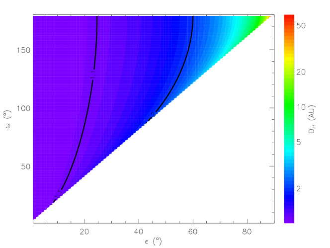
Based on the previous analysis, we found that the CME’s real propagating distance, , is determined by its angular width and the propagation direction. The propagating distance of the CME tip might be larger than 1 AU when the flank of the CME hit the Earth. To evaluate the influence of this effect, the values of with different angular widths and deviation angles were calculated. Assuming the deviation angle varied from 1∘ to 90∘ and the angular width varied from 1∘ to 180∘, Figure 8 shows the distribution of the values for the different cases. Note that the CMEs in the lower right half of the plot (, white regions in Figure 8) can not hit the Earth based on the SSE model. In other cases with , varied over a wide range, from 1 AU to more than 60 AU. Considering that a 10% uncertainty in the forecasting of the CME arrival time is acceptable, the influence of the different propagation direction and angular width on the travel time of a CME should be carefully considered in the cases with 1.1 AU. In a large fraction (60%) of the cases we discussed, the are larger than 1.1 AU, and those parameters must be considered. Inspecting Figure 8, one finds that at a given fixed value of , increases as the angular width decreases. Thus, the for narrower CMEs should be calculated first to forecast the arrival time of the CMEs. In addition, varies greatly with the change of the deviation angle, as shown in Figure 8. Larger values correspond to larger values. Figure 9 shows the maximum and minimum values of as a function of the deviation angle by assuming that the CME angular width varies from 1∘ to 180∘. It is found that both values increase with increasing . Particularly, when , the values of are always larger than 1.1 AU. Thus, combined with the previous results, we suggest that for narrow CMEs or the CME propagated with , the influence of the propagation direction and angular width on the CME’s transit distance is large, and the must be carefully calculated in the CME arrival time forecasting.

Acknowledgements.
We appreciate using of the CME catalog, the data from SECCHI instruments on STEREO and LASCO on SOHO. The CME catalog is generated and maintained at the CDAW Data Center by NASA and the Catholic University of America in cooperation with the Naval Research Laboratory. STEREO is the third mission in NASA Solar Terrestrial Probes program, and SOHO is a mission of international cooperation between ESA and NASA. We also thank the NSSDC at Goddard Space Flight Center/NASA for providing Wind and ACE data. The data for this paper are available at the official website of SOHO, STEREO, WIND and ACE satellites. The dataset we used are SOHO LASCO/C2, SOHO LASCO/C3, STEREO COR2, STEREO HI1, STEREO HI2, WIND MFI, WIND SWE and ACE SWEPAM. This work is supported by the Chinese Academy of Sciences (KZZD-EW-01), grants from the 973 key project 2011CB811403, NSFC 41131065, 41274173, 40874075, 41121003, and 41304145, CAS the 100-talent program, KZCX2-YW-QN511 and startup fund, and MOEC 20113402110001, the fundamental research funds for the central universities (WK2080000031) and the Strategic Priority Research Program on Space Science, the Chinese Academy of Sciences (Grant No. XDA04060801).References
- Cane et al. (2000) Cane, H. V., I. G. Richardson, and O. C. S. Cyr, Coronal mass ejections, interplanetray ejecta and geomagnetic storms, Geophysical Research Letters, 27(21), 3591–3594, 2000.
- Chen (1996) Chen, J., Theory of prominence eruption and propagation: Interplanetary consequences, Journal of Geophysical Research, 101(A), 27,499–27,520, 1996.
- Cremades and Bothmer (2004) Cremades, H., and V. Bothmer, On the three-dimensional configuration of coronal mass ejections, Astronomy and Astrophysics, 422(1), 307–322, 2004.
- Davies et al. (2012) Davies, J. A., et al., A Self-similar Expansion Model for Use in Solar Wind Transient Propagation Studies, Astrophysical Journal, 750(1), 23, 2012.
- Davis et al. (2009) Davis, C. J., J. A. Davies, M. Lockwood, A. P. Rouillard, C. J. Eyles, and R. A. Harrison, Stereoscopic imaging of an Earth‐impacting solar coronal mass ejection: A major milestone for the STEREO mission, Geophysical Research Letters, 36(8), L08,102, 2009.
- Feng and Zhao (2006) Feng, X., and X. Zhao, A New Prediction Method for the Arrival Time of Interplanetary Shocks, Solar Physics, 238(1), 167–186, 2006.
- Feng et al. (2007) Feng, X., Y. Zhou, and S. T. Wu, A novel numerical implementation for solar wind modeling by the modified conservation element/solution element method, Astrophysical Journal, 655, 1110, 2007.
- Feng et al. (2010) Feng, X., L. Yang, C. Xiang, S. T. Wu, Y. Zhou, and D. Zhong, Three-dimensional Solar WIND Modeling from the Sun to Earth by a SIP-CESE MHD Model with a Six-component Grid, Astrophysical Journal, 723(1), 300–319, 10.1088/0004-637X/723/1/300, 2010.
- Fry et al. (2003) Fry, C. D., M. Dryer, Z. Smith, W. Sun, C. S. Deehr, and S. I. Akasofu, Forecasting solar wind structures and shock arrival times using an ensemble of models, Journal of Geophysical Research, 108(A2), 1070, 2003.
- Gopalswamy and Thompson (2000) Gopalswamy, N., and B. J. Thompson, Early life of coronal mass ejections, Journal of Atmospheric and Solar-Terrestrial Physics, 62(16), 1457–1469, 2000.
- Gopalswamy et al. (2000) Gopalswamy, N., A. Lara, R. P. Lepping, M. L. Kaiser, D. Berdichevsky, and O. C. St Cyr, Interplanetary acceleration of coronal mass ejections, Geophysical Research Letters, 27, 145, 2000.
- Gopalswamy et al. (2001) Gopalswamy, N., A. Lara, S. Yashiro, M. L. Kaiser, and R. A. Howard, Predicting the 1-AU arrival times of coronal mass ejections, Journal of Geophysical Research, 106(A), 29,207–29,218, 2001.
- Gopalswamy et al. (2005) Gopalswamy, N., a. Lara, P. Manoharan, and R. Howard, An empirical model to predict the 1-AU arrival of interplanetary shocks, Advances in Space Research, 36(12), 2289–2294, 10.1016/j.asr.2004.07.014, 2005.
- Gopalswamy et al. (2007) Gopalswamy, N., S. Yashiro, and S. Akiyama, Geoeffectiveness of halo coronal mass ejections, Journal of Geophysical Research, 112(A), 6112, 2007.
- Gui et al. (2011) Gui, B., C. Shen, Y. Wang, P. Ye, and S. Wang, Quantitative Analysis of CME Deflections in the Corona, Solar Physics, 271, 111–139, 2011.
- Howard et al. (1982) Howard, R. A., D. J. Michels, N. R. SHEELEY, and M. J. Koomen, The Observation of a Coronal Transient Directed at Earth, Astrophysical Journal, 263(2), L101—-{&}, 1982.
- Howard et al. (2008) Howard, R. A., et al., Sun Earth Connection Coronal and Heliospheric Investigation (SECCHI), Space Science Reviews, 136(1), 67–115, 2008.
- Jian et al. (2006) Jian, L., C. T. Russell, J. G. Luhmann, and R. M. Skoug, Properties of Interplanetary Coronal Mass Ejections at One AU During 1995 – 2004, Solar Physics, 239(1-2), 337, 2006.
- Kilpua et al. (2009) Kilpua, E. K. J., J. Pomoell, A. Vourlidas, R. Vainio, J. Luhmann, Y. Li, P. Schroeder, A. B. Galvin, and K. Simunac, STEREO observations of interplanetary coronal mass ejections and prominence deflection during solar minimum period, Annales Geophysicae, 27(1), 4491–4503, 2009.
- Kim et al. (2005) Kim, R.-S., K.-S. Cho, Y.-J. Moon, Y.-H. Kim, Y. Yi, M. Dryer, S.-C. Bong, and Y.-D. Park, Forecast evaluation of the coronal mass ejection (CME) geoeffectiveness using halo CMEs from 1997 to 2003, Journal of Geophysical Research, 110(A11), A11,104, 2005.
- Lugaz and Kintner (2012) Lugaz, N., and P. Kintner, Effect of Solar Wind Drag on the Determination of the Properties of Coronal Mass Ejections from Heliospheric Images, Solar Physics, 2012.
- Lugaz et al. (2012) Lugaz, N., C. J. Farrugia, J. A. Davies, C. Möstl, C. J. Davis, I. I. Roussev, and M. Temmer, The Deflection of the Two Interacting Coronal Mass Ejections of 2010 May 23-24 as Revealed by Combined in Situ Measurements and Heliospheric Imaging, Astrophysical Journal, 759(1), 68, 2012.
- MacQueen et al. (1986) MacQueen, R. M., A. J. Hundhausen, and C. W. Conover, The propagation of coronal mass ejection transients, Journal of Geophysical Research, 91, 31, 1986.
- Maloney and Gallagher (2010) Maloney, S. A., and P. T. Gallagher, Solar Wind Drag and the Kinematics of Interplanetary Coronal Mass Ejections, The Astrophysical Journal Letters, 724(2), L127–L132, 2010.
- Mckenna-Lawlor et al. (2006) Mckenna-Lawlor, S. M. P., M. Dryer, M. D. Kartalev, Z. Smith, C. D. Fry, W. Sun, C. S. Deehr, K. Kecskemety, and K. Kudela, Near real-time predictions of the arrival at Earth of flare-related shocks during Solar Cycle 23, Journal of Geophysical Research, 111(A11), A11,103, 2006.
- Moon et al. (2005) Moon, Y., K. Cho, M. Dryer, Y. Kim, S. Bong, J. Chae, and Y. Park, New Geoeffective Parameters of Very Fast Halo Coronal Mass, American Geophysical Union, 23, 1, 2005.
- Möstl and Davies (2012) Möstl, C., and J. A. Davies, Speeds and Arrival Times of Solar Transients Approximated by Self-similar Expanding Circular Fronts, Solar Physics, 285(1-2), 411–423, 2012.
- Odstrcil (2003) Odstrcil, D., Modeling 3-D solar wind structure, Adv. Space Res., 32(4), 497–506, 2003.
- Odstrcil et al. (2004) Odstrcil, D., P. Riley, and X. P. Zhao, Numerical simulation of the 12 May 1997 interplanetary CME event, Journal of Geophysical Research, 109(A), 2116, 2004.
- Schwenn et al. (2005) Schwenn, R., A. Dal Lago, E. Huttunen, and W. D. Gonzalez, The association of coronal mass ejections with their effects near the Earth, Annales Geophysicae, 23(3), 1033–1059, 2005.
- Shanmugaraju and Vršnak (2014) Shanmugaraju, A., and B. Vršnak, Transit Time of Coronal Mass Ejections under Different Ambient Solar Wind Conditions, Solar Physics, 289, 339–349, 10.1029/2001/JA000120, 2014.
- Sheeley et al. (1999) Sheeley, N. R., J. H. Walters, Y. M. Wang, and R. A. Howard, Continuous tracking of coronal outflows: Two kinds of coronal mass ejections, Journal of Geophysical Research, 104(A), 24,739–24,768, 1999.
- Shen et al. (2011) Shen, C., Y. Wang, B. Gui, P. Ye, and S. Wang, Kinematic Evolution of a Slow CME in Corona Viewed by STEREO-B on 8 October 2007, Solar Physics, 269(2), 389–400, 2011.
- Shen et al. (2013) Shen, C., Y. Wang, Z. Pan, M. Zhang, P. Ye, and S. Wang, Full halo coronal mass ejections: Do we need to correct the projection effect in terms of velocity?, Journal of Geophysical Research: Space Physics, 118, 6858–6865, 10.1002/2013JA018872, 2013.
- Shen et al. (2012) Shen, C., et al., Super-elastic collision of large-scale magnetized plasmoids in the heliosphere, Nature Physics, 8(1), 923–928, 2012.
- Shen et al. (2007) Shen, F., X. Feng, S. T. Wu, and C. Xiang, Three-dimensional MHD simulation of CMEs in three-dimensional background solar wind with the self-consistent structure on the source surface as input: Numerical simulation of the January 1997 Sun-Earth connection event, Journal of Geophysical Research, 112(A6), 6109, 2007.
- Shen et al. (2010) Shen, F., X. Feng, C. Xiang, and W. Song, The statistical and numerical study of the global distribution of coronal plasma and magnetic field near 2.5Rs over a 10-year period, Journal of Atmospheric and Solar-Terrestrial Physics, 72(13), 1008–1018, 2010.
- Svalgaard and Kamide (2013) Svalgaard, L., and Y. Kamide, Asymmetric Solar Polar Field Reversals, The Astrophysical Journal, 763(1), 23, 2013.
- Temmer et al. (2011) Temmer, M., T. Rollett, C. Möstl, A. M. Veronig, B. Vršnak, and D. Odstrcil, Influence of the Ambient Solar Wind Flow on the Propagation Behavior of Interplanetary Coronal Mass Ejections, Astrophysical Journal, 743(2), 101, 2011.
- Thernisien (2011) Thernisien, A., Implementation of the Graduated Cylindrical Shell Model for the Three-dimensional Reconstruction of Coronal Mass Ejections, The Astrophysical Journal Supplement Series, 194, 33, 2011.
- Thernisien et al. (2009) Thernisien, A., A. Vourlidas, and R. A. Howard, Forward Modeling of Coronal Mass Ejections Using STEREO/SECCHI Data, Solar Physics, 256(1), 111–130, 2009.
- Thernisien et al. (2006) Thernisien, A. F. R., R. A. Howard, and A. Vourlidas, Modeling of Flux Rope Coronal Mass Ejections, Astrophysical Journal, 652, 763, 2006.
- Tóth et al. (2005) Tóth, G., et al., Space Weather Modeling Framework: A new tool for the space science community, Journal of Geophysical Research, 110(A12), 2005.
- Vršnak and Žic (2007) Vršnak, B., and T. Žic, Transit times of interplanetary coronal mass ejections and the solar wind speed, Astronomy and Astrophysics, 472(3), 937–943, 10.1051/0004-6361:20077499, 2007.
- Vršnak et al. (2013) Vršnak, B., et al., Propagation of Interplanetary Coronal Mass Ejections: The Drag-Based Model, Solar Physics, 285(1-2), 295–315, 2013.
- Wang et al. (2004) Wang, Y., C. Shen, S. Wang, and P. Ye, Deflection of coronal mass ejection in the interplanetary medium, Solar Physics, 222, 329, 2004.
- Wang et al. (2006) Wang, Y., X. Xue, C. Shen, P. Ye, S. Wang, and J. Zhang, Impact of Major Coronal Mass Ejections on Geospace during 2005 September 7-13, Astrophysical Journal, 646, 625, 2006.
- Wang et al. (2011) Wang, Y., C. Chen, B. Gui, C. Shen, P. Ye, and S. Wang, Statistical study of coronal mass ejection source locations: Understanding CMEs viewed in coronagraphs, Journal of Geophysical Research, 116(A4), A04,104, 2011.
- Wang et al. (2013) Wang, Y., B. Wang, C. Shen, and F. Shen, Deflected propagation of a coronal mass ejection from the corona to interplanetary space, Journal of Geophysical Research : Space Physics, p. Submitted, 2013.
- Wang et al. (2002) Wang, Y. M., P. Z. Ye, S. Wang, G. P. Zhou, and J. X. Wang, A statistical study on the geoeffectiveness of Earth-directed coronal mass ejections from March 1997 to December 2000, Journal of Geophysical Research, 107(A11), 1340, 2002.
- Webb (2002) Webb, D. F., CMEs and the solar cycle variation in their geoeffectiveness, In: Proceedings of the SOHO 11 Symposium on From Solar Min to Max: Half a Solar Cycle with SOHO, 508, 409, 2002.
- Xiong et al. (2009) Xiong, M., H. Zheng, and S. Wang, Magnetohydrodynamic simulation of the interaction between two interplanetary magnetic clouds and its consequent geoeffectiveness: 2. Oblique collision, Journal of Geophysical Research, 114(A), 11,101, 2009.
- Yashiro et al. (2004) Yashiro, S., N. Gopalswamy, G. Michalek, O. C. St Cyr, S. P. Plunkett, N. B. Rich, and R. A. Howard, A catalog of white light coronal mass ejections observed by the SOHO spacecraft, Journal of Geophysical Research, 109(A), 7105, 2004.
- Yermolaev and Yermolaev (2006) Yermolaev, Y. I., and M. Y. Yermolaev, Statistic study on the geomagnetic storm effectiveness of solar and interplanetary events, Advances in Space Research, 37(6), 1175–1181, 2006.
- Zhang et al. (2003) Zhang, J., K. P. Dere, R. A. Howard, and V. Bothmer, Identification of Solar Sources of Major Geomagnetic Storms between 1996 and 2000, Astrophysical Journal, 582(1), 520–533, 2003.
- Zhang et al. (2007) Zhang, J., et al., Solar and interplanetary sources of major geomagnetic storms ( Dst≤ −100 nT) during 1996–2005, Journal of Geophysical Research, 112(A10), A10,102, 2007.
- Zhao and Webb (2003) Zhao, X. P., and D. F. Webb, Source regions and storm effectiveness of frontside full halo coronal mass ejections, Journal of Geophysical Research, 108(A6), 1234, 2003.
- Zhou and Feng (2013) Zhou, Y. F., and X. S. Feng, MHD numerical study of the latitudinal deflection of coronal mass ejection, Journal of Geophysical Research, 118(10), 6007–6018, 2013.