Abstract

Phylogenetic analyses which include fossils or molecular sequences that are sampled through time require models that allow one sample to be a direct ancestor of another sample. As previously available phylogenetic inference tools assume that all samples are tips, they do not allow for this possibility.

We have developed and implemented a Bayesian Markov Chain Monte Carlo (MCMC) algorithm to infer what we call sampled ancestor trees, that is, trees in which sampled individuals can be direct ancestors of other sampled individuals.

We use a family of birth-death models where individuals may remain in the tree process after the sampling, in particular we extend the birth-death skyline model [Stadler et al, 2013] to sampled ancestor trees. This method allows the detection of sampled ancestors as well as estimation of the probability that an individual will be removed from the process when it is sampled. We show that sampled ancestor birth-death models where all samples come from different time points are non-identifiable and thus require one parameter to be known in order to infer other parameters.

We apply this method to epidemiological data, where the possibility of sampled ancestors enables us to identify individuals that infected other individuals after being sampled and to infer fundamental epidemiological parameters.

We also apply the method to infer divergence times and diversification rates when fossils are included among the species samples, so that fossilisation events are modelled as a part of the tree branching process. Such modelling has many advantages as argued in literature.

The sampler is available as an open-source BEAST2 package
(https://github.com/gavryushkina/sampled-ancestors).

Author Summary

A central goal of phylogenetic analysis is to estimate evolutionary relationships and population parameters such as speciation and extinction rates or the rate of infectious disease spread from molecular data. The statistical methods used in these analyses require that the underlying tree branching process be specified. Standard models for the branching process which were originally designed to describe the evolutionary past of present day species do not allow for direct ancestors within the sampled taxa, that is, they do not allow one sampled taxon to be the ancestor of another. However the probability of sampling a direct ancestor is not negligible for many types of data. For example, when fossil and living species are analysed together to infer species divergence times, fossil species may or may not be direct ancestors of living species. In epidemiology, a sampled individual (a host from which a pathogen sequence was obtained) can infect other individuals after sampling, which then go on to be sampled themselves. Recently, models that allow for direct ancestors have been introduced. Such models produce phylogenetic trees with a different structure from the classic phylogenetic trees and so using these models in inference requires new computational methods. Here we developed and implemented a Bayesian Markov chain Monte Carlo framework for phylogenetic analysis allowing for the possibility of direct ancestors.

Introduction

Phylogenetic analysis uses molecular sequence data to infer evolutionary relationships between organisms and to infer evolutionary parameters. Since the introduction of Bayesian inference in phylogenetics [1, 2, 3], it has become the standard approach for fully probabilistic inference of evolutionary history with many popular implementations [4, 5, 6, 7] of Markov chain Monte Carlo (MCMC) [8, 9] sampling over the space of phylogenetic trees. Initial descriptions of Bayesian phylogenetic analysis were restricted to considering bifurcating trees [1, 2], but have been extended to include explicit polytomies [10]. Here we tackle phylogenetic inference with trees that may contain sampled ancestors [11].

Standard phylogenetic models developed for inferring the evolutionary past of present day species assume that all samples are terminal (leaf) nodes in the estimated phylogenetic tree. However, serially sampled data generated by different evolutionary processes can be analysed using phylogenetic methods [12] and, in some cases, the assumption that all sampled taxa are leaf nodes is not appropriate.

One case in point is when inferring epidemiological parameters from viral sequence data obtained from infected hosts [13, 14, 15, 16, 17]. Viral sequences are obtained from distinct hosts and treated as samples from the transmission process. Using standard models to describe the infectious disease transmission process entails the assumption that a host becomes uninfectious at sampling (where sampling is obtaining a sequence or sequences from the pathogen population residing in a single infected host). However in many cases, hosts remain infectious after sampling and, when sampling is sufficiently dense, the probability of sampling an individual that later infects another individual which is also sampled is not negligible [18, 19, 20].

A recent analysis of a well-characterised HIV transmission chain [20] employed a hierarchical model of a gene tree inside a transmission tree to infer the differences in evolutionary rates (substitution rates) within and among hosts. Hierarchical modelling of gene trees inside transmission trees has also been used to infer transmission events for small epidemic outbreaks where epidemiological data is available in the form of known infection and recovery times for each host [16]. In both cases the inference of transmission trees assumes complete sampling of the hosts involved, and the host sampling process is not explicitly modelled.

Incomplete sampling is explicitly modelled by birth-death-sampling models [21, 15, 22, 23], for which the probability density functions of the trees are available in closed form, thus making these models tractable for use in Bayesian inference. The birth-death-sampling models do not assume that individuals are removed from the tree process after the sampling. However, applications of models allowing for infection after sampling has not been possible due to a lack of software, meaning that many applications simply ignore sampled ancestors [15, 23].

Another problem that may require sampled ancestor models is inferring species divergence times using fossil data. Without the means to calibrate the times of divergences, the length of branches in the estimated molecular phylogeny of contemporaneous sequences are typically described in units of expected substitutions per site. Geologically dated fossil data can be employed to calibrate a phylogenetic tree, thus providing absolute branch lengths. The most common approach here is to specify age limits or a probability density function on specific divergence times in the phylogeny, where the constraints are defined using the fossil data [24, 25, 26, 27, 28]. There are several drawbacks connected to this approach [29, 30]. First, there is potential for inconsistency when applying two priors on the phylogeny [31]: a calibration prior on one or more divergence times and a tree process prior on the entire tree. Second, it is not obvious how to specify a calibration density so that it reflects prior knowledge about divergence times [29, 30]. Finally, such densities usually only use the oldest fossil within a particular clade, thus discarding much of the information available in the fossil record [30].

An approach that addresses these issues requires modelling fossilisation events as a part of the tree process prior. This allows for the joint analysis of fossil and recent taxa together in a unified framework [32, 33, 29, 30, 34]. Models that jointly describe the processes of macroevolution and fossilisation should account for possible ancestor-descendant relationships between fossil and living species [35], and thus include sampled ancestors.

A birth-death model with sampled ancestors have been used to estimate speciation and extinction rates from phylogenies in [22]. Heath et al. [30] have used the birth-death model with sampled ancestors (they call this the fossilized birth-death process) to explicitly model fossilisation events and estimate divergence times in a Bayesian framework. In their approach, the tree topology relating the extant species has to be known for the inference [30]. So a method that simultaneously estimates the divergence times and tree topology while modelling incorporation of sampled fossil taxa is an obvious next step.

Full Bayesian MCMC inference using models with sampled ancestors is complicated by the fact that such models produce trees, which we call sampled ancestor trees [11], that are not strictly binary. They may have sampled nodes that lie on branches, forming an internal node with one direct ancestor and one direct descendent. Thus, modelling sampled ancestors induces a tree space where the tree has a variable number of dimensions (a function of the number of sampled ancestors), which necessitates extensions to the standard MCMC tree algorithms.

Here we describe a reversible-jump MCMC proposal kernel [36] to effectively traverse the space of sampled ancestor trees and implement it within the BEAST2 software platform [6]. We study the limitations of birth-death models with sampled ancestors and extend the birth-death skyline model [23] to sampled ancestor trees. We apply the new posterior sampler to two types of data: a serially sampled viral data set (from HIV), and molecular phylogeny of bear sequences with fossil samples.

Methods

Tree models with sampled ancestors

In this section, we consider birth-death sampling models [21, 15, 22, 23] under the assumption that sampled individuals are not necessarily removed from the process at sampling. This results in a type of phylogenetic tree that may contain degree two nodes called sampled ancestors.

An important characteristic of the models we consider here is incomplete sampling, i.e., we only observe a part of the tree produced by a process. Consider a birth-death process that starts at some point in time (the time of origin) with one lineage and then each existing lineage may bifurcate or go extinct. Further, the lineages are randomly sampled through time. An example of a full tree produced by such process is shown in Figure 1 on the left. We have information only about the portion of the process that produces the samples, shown as labeled nodes, and do not observe the full tree. Thus we only consider this subtree relating to the sample, which is called the reconstructed tree (or the sampled tree) and is shown on the right of Figure 1.

The sampled ancestor birth-death model

Here we describe a serially-sampled birth-death model with sampled ancestors [21, 15].

The process begins at the time of origin $t_{or}>0$ measured in time units before the present. Moving towards the present, each existing lineage bifurcates or goes extinct according to two independent Poisson processes with constant rates $\lambda$ and $\mu$, respectively. Concurrently, each lineage is sampled with Poisson rate $\psi$ and is removed from the process at sampling with probability $r$. The process is stopped at time $0$. This process can be used to model the transmission of infectious disease and we call it the transmission birth-death process.

The transmission process produces trees that have degree two nodes corresponding to sampling events when a lineage was sampled but was not removed. We call these trees sampled ancestor trees (whether or not any sampled ancestors are present). The reconstructed tree has degree-two nodes when a lineage is sampled but not removed and then it, or a descendent lineage, is sampled again. The reconstructed tree in Figure 1 (on the right) is an example of a sampled ancestor tree. Note that the root of a sampled ancestor tree is the most recent common ancestor of the sampled nodes and therefore it may be a sampled node. There is no origin node in the tree because the time of origin is a model parameter and not an outcome of the process.

A tree (or genealogy) $g$ consists of the discrete component $\mathcal{T}$, which is called a tree topology, and the continuous component $\bar{\tau}$, which is called a time vector. The tree topology of a sampled ancestor tree is a sampled ancestor phylogenetic tree, which is a ranked labeled phylogenetic tree with labeled degree-two vertices (a rigorous definition of a sampled ancestor phylogenetic tree can be found in [11], where it is called an FRS tree). The time vector is a real-valued vector of the same dimension as the number of ranks (nodes) in the tree topology and with coordinates going in the descending order so that each node in the tree topology can be unambiguously assigned a time from the time vector.

Further, we have three types of nodes: bifurcation nodes, sampled tip nodes, sampled internal nodes. Let $m$ be the number of leaves, then $m-1$ is the number of bifurcation events. Let $\bar{x}=(x_{1},\ldots,x_{m-1})$ be a vector of bifurcation times, where $x_{m-1}<\ldots<x_{1}$. Let $\bar{y}=(y_{1},\ldots,y_{m})$ be a vector of tip times, where $y_{m}<\ldots<y_{1}$. Further let $\bar{z}=(z_{1},\ldots,z_{k})$ be a vector of times of sampled two degree nodes, where $z_{k}<\ldots<z_{1}$ and $k$ is the number of such nodes. Then $\bar{\tau}$ can be obtained by combining elements of $\bar{x}$, $\bar{y}$, and $\bar{z}$ and ordering them in the descending order (see also Figure 1). A genealogy may be written as $(\mathcal{T},\bar{x},\bar{y},\bar{z})$.

Stadler et al. [15] derive the density of a genealogy $g=(\mathcal{T},\bar{x},\bar{y},\bar{z})$ given the transmission birth-death process parameters $\lambda,\mu,\psi,r$ and time of origin $t_{or}$. In [21], it was indicated that we should also condition on the event, $S$, of sampling at least one individual because only non-empty samples are observed. The density is

$$f[g|\lambda,\mu,\psi,r,t_{or},S]=\frac{1}{(m+k)!}\frac{(\psi(1-r))^{k}q(t_{or})}{1-p_{0}(t_{or})}\prod_{i=1}^{m-1}2\lambda q(x_{i})\prod_{i=1}^{m}\frac{\psi(r+(1-r)p_{0}(y_{i}))}{q(y_{i})},$$ (1)

where the function $p_{0}(x)$ is the probability that an individual has no sampled descendants for a time span of length $x$ so that

$$p_{0}(x)=\frac{\lambda+\mu+\psi+c_{1}\frac{e^{-c_{1}x}(1-c_{2})-(1+c_{2})}{e^{-c_{1}x}(1-c_{2})+(1+c_{2})}}{2\lambda}$$

where

$$c_{1}=|\sqrt{(\lambda-\mu-\psi)^{2}+4\lambda\psi}|,\quad c_{2}=-\frac{\lambda-\mu-\psi}{c_{1}}$$

and

$$q(x)=\frac{4}{2(1-c_{2}^{2})+e^{-c_{1}x}(1-c_{2})^{2}+e^{c_{1}x}(1+c_{2})^{2}}.$$

Throughout this paper, we consider non-oriented labeled trees. So equation (1) differs from the equation on page 350 in [15], written for oriented trees, by a factor accounting for the switch from oriented to labeled trees and also by the term for conditioning on $S$. Note also that the definition of the function $q$ here is different from the definition in [15].

We show in the Supporting Information that function (1) depends only on three parameters: $\lambda-\mu-\psi$, $\lambda\psi$, and $\psi(1-r)$, and does not depend on parameters $\lambda$, $\mu$, $\psi$ and $r$ independently. This means that the tree model is unidentifiable but, as we show in simulation studies, if we specify one of the parameters we can estimate the others.

When applying this model to data, we typically shift time such that the most recent tip occurs at present, $y_{m}=0$, as we often do not have information about the length of time between the last sample and the end of the sampling effort. This is done to reduce our set of unknown quantities by one (namely setting $y_{m}=0$).

We extend the model to allow the possibility of sampling individuals at present, where each lineage at time 0 is sampled with probability $\rho$. This process, with $r$ set to zero, can be used to model speciation processes with fossilisation events, hence it is called the fossilized birth-death process [30]. Let $S_{\rho}$ denote the event of sampling at least one individual at present then according to [21] and accounting for labeled trees:

$$f[g|\lambda,\mu,\psi,\rho,t_{or},S_{\rho}]=\frac{1}{(m+k)!}\frac{\psi^{k}\rho^{n}q(t_{or})}{1-\hat{p}_{0}(t_{or})}\prod_{i=1}^{m+n-1}2\lambda q(x_{i})\prod_{i=1}^{m}\frac{\psi p_{0}(y_{i})}{q(y_{i})}$$ (2)

where $n$ is the number of $\rho$-sampled tips and

$$\hat{p}_{0}(t_{or})=1-\frac{\rho(\lambda-\mu)}{\lambda\rho+(\lambda(1-\rho)-\mu)e^{-(\lambda-\mu)t}}.$$

In contrast to the transmission birth-death process, where only three out of the four parameters $\lambda$, $\mu$, $\psi$, and $r$ can be inferred, under the fossilized birth-death process, all four parameters $\lambda$, $\mu$, $\psi$, and $\rho$ can be identified from the phylogeny.

It is possible to re-write density (2) conditioning on the time of the most recent common ancestor of sampled individuals rather than conditioning on the time of origin. In this case, we discard trees in which the root is a sampled node. In other words, we assume that the process starts with a bifurcation event and we only consider trees with sampled nodes on both sides of the initial bifurcation event. Then the time of the most recent common ancestor of the sample is the time of the root, $x_{1}$. Accounting for labeled trees, the probability density function can thus be written [21] as:

$$f[g|\lambda,\mu,\psi,\rho,x_{1},S_{\rho}]=\frac{1}{(m+k)!}\frac{\psi^{k}\rho^{n}q(x_{1})}{\lambda(1-\hat{p}_{0}(x_{1}))^{2}}\prod_{i=1}^{m+n-1}2\lambda q(x_{i})\prod_{i=1}^{m}\frac{\psi p_{0}(y_{i})}{q(y_{i})}.$$ (3)

The sampled ancestor skyline model

Here we extend the sampled ancestor birth-death model so that parameters may change through time in a piecewise manner. This model combines two models from [15] and [23].

Let there be $l$ time intervals $[t_{i},t_{i-1})$ for $i\in\{1,\ldots,l\}$ defined by vector $\bar{t}=(t_{0},\ldots,t_{l-1})$ and $t_{l}=0$ with $t_{l}<t_{l-1}<\ldots<t_{1}<t_{0}$ (where $t_{0}$ plays the role of the origin time, i.e., $t_{or}=t_{0}$). We use notation $t_{l}$ for time zero only for convenience and do not include it as a model parameter. Within each interval $[t_{i},t_{i-1})$, $i\in\{1,\ldots,l\}$ the constant birth-death parameters $\lambda_{i}$, $\mu_{i}$, $\psi_{i}$, and $r_{i}$ apply. At the end of each interval at times $t_{i}$, $i\in\{1,\ldots,l\}$, each individual may be sampled with probability $\rho_{i}$ (see also Figure 1). Thus, the model has $6l$ parameters: $\bar{\lambda}$, $\bar{\mu}$, $\bar{\psi}$, $\bar{r}$, $\bar{\rho}$, and $\bar{t}$. We prove in the Supporting Information that the probability density of a reconstructed sampled ancestor tree $g=(\mathcal{T}|\bar{x},\bar{y},\bar{z})$ produced by this process is (not conditioned on survival),

$$\begin{multlined}f[g|\bar{\lambda},\bar{\mu},\bar{\psi},\bar{r},\bar{\rho},\bar{t}]=\frac{1}{(m+M+k+K)!}\times\\ q_{1}(t_{0})\prod_{i=1}^{k}(1-r_{\mathbf{i}_{z_{i}}})\psi_{\mathbf{i}_{z_{i}}}\prod_{i=1}^{m+M-1}2\lambda_{\mathbf{i}_{x_{i}}}q_{\mathbf{i}_{x_{i}}}(x_{i})\prod_{i=1}^{m}\frac{\psi_{\mathbf{i}_{y_{i}}}(r_{\mathbf{i}_{y_{i}}}+(1-r_{\mathbf{i}_{y_{i}}})p_{\mathbf{i}_{y_{i}}}(y_{i}))}{q_{\mathbf{i}_{y_{i}}}(y_{i})}\times\\ \prod_{i=1}^{l}((1-\rho_{i})q_{i+1}(t_{i}))^{n_{i}}\rho_{i}^{N_{i}}((1-r_{i+1})q_{i+1}(t_{i}))^{K_{i}}(r_{i+1}+(1-r_{i+1})p_{i+1}(t_{i}))^{M_{i}}\end{multlined}f[g|\bar{\lambda},\bar{\mu},\bar{\psi},\bar{r},\bar{\rho},\bar{t}]=\frac{1}{(m+M+k+K)!}\times\\ q_{1}(t_{0})\prod_{i=1}^{k}(1-r_{\mathbf{i}_{z_{i}}})\psi_{\mathbf{i}_{z_{i}}}\prod_{i=1}^{m+M-1}2\lambda_{\mathbf{i}_{x_{i}}}q_{\mathbf{i}_{x_{i}}}(x_{i})\prod_{i=1}^{m}\frac{\psi_{\mathbf{i}_{y_{i}}}(r_{\mathbf{i}_{y_{i}}}+(1-r_{\mathbf{i}_{y_{i}}})p_{\mathbf{i}_{y_{i}}}(y_{i}))}{q_{\mathbf{i}_{y_{i}}}(y_{i})}\times\\ \prod_{i=1}^{l}((1-\rho_{i})q_{i+1}(t_{i}))^{n_{i}}\rho_{i}^{N_{i}}((1-r_{i+1})q_{i+1}(t_{i}))^{K_{i}}(r_{i+1}+(1-r_{i+1})p_{i+1}(t_{i}))^{M_{i}}$$ (4)

where $m$ is the number of $\psi$-sampled tips; $k$ is the number of $\psi$-sampled nodes that have sampled descendants; $M_{i}$ is the number of tips sampled at time $t_{i}$; $K_{i}$ is the number of nodes sampled at time $t_{i}$ and having sampled descendants; $N_{i}=K_{i}+M_{i}$ is the total number of nodes sampled at time $t_{i}$; $n_{i}$ is the number of lineages present in the tree at time $t_{i}$ but not sampled at this time for $i~{}\in~{}\{1,\ldots,l\}$; $M=\sum\limits_{i=1}^{l}M_{i}$; $K=\sum\limits_{i=1}^{l}K_{i}$; ${\bf i}_{x}$ is an index such that $t_{{\bf i}_{x}}\leq x<t_{{\bf i}_{x}-1}$; and functions $p_{i}$ and $q_{i}$ are defined presently.

The probability $p_{i}(t)$ that an individual alive at time $t$ has no sampled descendants when the process is stopped (i.e., in the time interval $[t_{l},t]$), with $t_{i}\leq t<t_{i-1}$ ($i=1,\ldots,l$) is

$$p_{i}(t)=\frac{\lambda_{i}+\mu_{i}+\psi_{i}-A_{i}\frac{e^{A_{i}(t-t_{i})}(1+B_{i})-(1-B_{i})}{e^{A_{i}(t-t_{i})}(1+B_{i})+(1-B_{i})}}{2\lambda_{i}}$$

where

$$A_{i}=\sqrt{(\lambda_{i}-\mu_{i}-\psi_{i})^{2}+4\lambda_{i}\psi_{i}}$$

and

$$B_{i}=\frac{(1-2(1-\rho_{i})p_{i+1}(t_{i}))\lambda_{i}+\mu_{i}+\psi_{i}}{A_{i}}$$

for $i=1,\ldots,l$ and $p_{l+1}(t_{l})=1$. Further,

$$q_{i}(t)=\frac{4e^{A_{i}(t-t_{i})}}{(e^{A_{i}(t-t_{i})}(1+B_{i})+(1-B_{i}))^{2}}$$

for $i=1,\ldots,l$. Note that $q_{l+1}(t_{l})$ does not appear in the equation because $n_{l}$ (which is the number of lineages present in the tree at time $t_{l}$ but not sampled at that time) and $K_{l}$ (which is the number of two degree nodes at time $t_{l}$) are always zero. Also, $r_{l+1}$ cancels out because $K_{l}$ is always zero and $p_{l+1}(t_{l})=1$.

We obtain two special cases of this general model that correspond to the skyline variants of the transmission and fossilized birth-death processes by setting some of the parameters to zero.

To obtain the skyline transmission process, we set $\bar{\rho}=0$. This implies $K_{i}=0$, $M_{i}=0$, and $N_{i}=0$ for all $i$. As before, we condition on the event, $S$, of sampling at least one individual, where $f[S|\bar{\lambda},\bar{\mu},\bar{\psi},\bar{t}]=1-p_{1}(t_{0})$. The tree density is

$$\begin{multlined}f[g|\bar{\lambda},\bar{\mu},\bar{\psi},\bar{r},\bar{t},S]=\frac{1}{(m+M+k+K)!}\times\\ \frac{q_{1}(t_{0})}{1-p_{1}(t_{0})}\prod_{i=1}^{k}(1-r_{\mathbf{i}_{z_{i}}})\psi_{\mathbf{i}_{z_{i}}}\prod_{i=1}^{m-1}2\lambda_{\mathbf{i}_{x_{i}}}q_{\mathbf{i}_{x_{i}}}(x_{i})\prod_{i=1}^{m}\frac{\psi_{\mathbf{i}_{y_{i}}}(r_{\mathbf{i}_{y_{i}}}+(1-r_{\mathbf{i}_{y_{i}}})p_{\mathbf{i}_{y_{i}}}(y_{i}))}{q_{\mathbf{i}_{y_{i}}}(y_{i})}\prod_{i=1}^{l}(q_{i+1}(t_{i}))^{n_{i}}\end{multlined}f[g|\bar{\lambda},\bar{\mu},\bar{\psi},\bar{r},\bar{t},S]=\frac{1}{(m+M+k+K)!}\times\\ \frac{q_{1}(t_{0})}{1-p_{1}(t_{0})}\prod_{i=1}^{k}(1-r_{\mathbf{i}_{z_{i}}})\psi_{\mathbf{i}_{z_{i}}}\prod_{i=1}^{m-1}2\lambda_{\mathbf{i}_{x_{i}}}q_{\mathbf{i}_{x_{i}}}(x_{i})\prod_{i=1}^{m}\frac{\psi_{\mathbf{i}_{y_{i}}}(r_{\mathbf{i}_{y_{i}}}+(1-r_{\mathbf{i}_{y_{i}}})p_{\mathbf{i}_{y_{i}}}(y_{i}))}{q_{\mathbf{i}_{y_{i}}}(y_{i})}\prod_{i=1}^{l}(q_{i+1}(t_{i}))^{n_{i}}$$ (5)

We show in the Supporting Information that (5) can be re-parameterised with

$$d_{i}=\lambda_{i}-\mu_{i}-\psi_{i} i=1,\ldots,l$$ for (6)

$$f_{i}=\lambda_{i}\psi_{i} i=1,\ldots,l$$ for

$$g_{i}=(1-r_{i})\psi_{i} i=1,\ldots,l,\mbox{ and}$$ for

$$k_{i}=\frac{\lambda_{i}}{\lambda_{i+1}} i=1,\ldots,l-1.$$ for

Thus, of the original $4l$ parameters, only $4l-1$ may be estimated.

For the skyline fossilized birth-death model, we set $\rho_{1},\ldots,\rho_{l-1}=0$ and $\bar{r}=0$ and condition on $S_{\rho}$, the event of sampling at least one extant individual (i.e., at time $t_{l}$). The tree density becomes

$$\begin{multlined}f[g|\bar{\lambda},\bar{\mu},\bar{\psi},\rho_{l},\bar{t},S_{\rho}]=\frac{1}{(m+M+k+K)!}\times\\ \rho_{l}^{N_{l}}\frac{q_{1}(t_{0})}{1-\hat{p}_{1}(t_{0})}\prod_{i=1}^{k}\psi_{\mathbf{i}_{z_{i}}}\prod_{i=1}^{m+N_{l}-1}2\lambda_{\mathbf{i}_{z_{i}}}q_{\mathbf{i}_{x_{i}}}(x_{i})\prod_{i=1}^{m}\frac{\psi_{\mathbf{i}_{y_{i}}}p_{\mathbf{i}_{y_{i}}}(y_{i})}{q_{\mathbf{i}_{y_{i}}}(y_{i})}\prod_{i=1}^{l}(q_{i+1}(t_{i}))^{n_{i}}\end{multlined}f[g|\bar{\lambda},\bar{\mu},\bar{\psi},\rho_{l},\bar{t},S_{\rho}]=\frac{1}{(m+M+k+K)!}\times\\ \rho_{l}^{N_{l}}\frac{q_{1}(t_{0})}{1-\hat{p}_{1}(t_{0})}\prod_{i=1}^{k}\psi_{\mathbf{i}_{z_{i}}}\prod_{i=1}^{m+N_{l}-1}2\lambda_{\mathbf{i}_{z_{i}}}q_{\mathbf{i}_{x_{i}}}(x_{i})\prod_{i=1}^{m}\frac{\psi_{\mathbf{i}_{y_{i}}}p_{\mathbf{i}_{y_{i}}}(y_{i})}{q_{\mathbf{i}_{y_{i}}}(y_{i})}\prod_{i=1}^{l}(q_{i+1}(t_{i}))^{n_{i}}$$ (7)

where

$$\hat{p}_{1}(t)=p_{1}(t|\bar{\psi}=0).$$

This probability density can be re-parameterised as in (6) with one additional equation $h=\lambda_{l}\rho_{l}$ (see Supporting Information). Now there are $3l+1$ initial parameters: $\bar{\lambda}$, $\bar{\mu}$, $\bar{\psi}$, and $\rho_{l}$ and $4l$ equations defining the re-parameterisation. Since $r_{i}=0$, $g_{i}$ defines $\psi_{i}$, then $f_{i}$ yields $\lambda_{i}$, then $d_{i}$ yields $\mu_{i}$, $h$ yields $\rho_{l}$ and the $l-1$ equations for $k_{i}$ are not needed at all, thus $3l+1$ equations define the reparameterization of the $3l+1$ parameters, thus this re-parameterisation does not reduce the number of parameters.

Markov chain Monte Carlo Operators

We introduce a number of operators to explore the space of sampled ancestor trees with a fixed number of sampled nodes. Throughout this section, we denote the height (or the age) of a node $a$ by $\tau_{a}$.

Extension of Wilson Balding operator

We extend the Wilson Balding operator (a type of subtree prune and regraft) [37] to sampled ancestor trees so that it is identical to the original operator when it is restricted to trees with no sampled ancestors. The operator may propose a significant change to a tree and may change its dimension, that is, the number of nodes in the tree. We use the reversible jump formalism of [36].

First, we describe a reduced version of the operator that does not change the root. Let $g=(\mathcal{T},\bar{\tau})$ be a genealogy. There are three steps in proposing a new tree.

1. Choose edge $e_{1}=\langle p_{1},c_{1}\rangle$ uniformly at random such that $p_{1}$ is not the root ($p_{1}$ is the parent of $c_{1}$). Recall that we do not consider the origin as a node belonging to the tree.

2. Choose either edge $e_{2}=\langle p_{2},c_{2}\rangle$ or leaf $l$. The method of selection depends on the type of $e_{1}$:

   1. if node $c_{1}$ has a sibling then, uniformly at random from all possibilities, either choose edge $e_{2}$ which is not adjacent to $e_{1}$ and at least one end of which is above $c_{1}$ (i.e., $p_{2}$ is older than $c_{1}$) or leaf $l$ which is older than $c_{1}$;

   2. if node $c_{1}$ does not have a sibling (so $p_{1}$ is a sampled node) then choose edge $e_{2}$ such that at least one of its ends is older than $c_{1}$ or a leaf which is older than $c_{1}$ uniformly at random.

   If there is no such edge nor leaf, do nothing and propose no new tree.

3. If an item was chosen in step 2, then prune the subtree rooted at node $p_{1}$ and reattach it to edge $e_{2}$ or leaf $l$. When attaching to an edge, we draw a new height for the parent of node $c_{1}$ uniformly at random from the interval $[\max(\tau_{c_{1}},\tau_{c_{2}}),\tau_{p_{2}}]$.

Figure 2 illustrates pruning from a branch (case 2a) and from a node (case 2b) and attaching to a branch and to a leaf. Let the resulting new genealogy be $g^{*}=(\mathcal{T}^{*},\bar{\tau}^{*})$.

Now we extend this move to add the possibility of changing the root. We modify the described procedure in two ways. First, we allow to choose $e_{1}$ for which $p_{1}$ is the root at the first step. Second, we can also choose the root edge at the second step, i.e., the edge which connects the root with the origin. Although we do not usually consider this edge as a part of the tree, for convenience we assume we can choose it. In this case, the parent of node $c_{1}$ becomes a new root with the height obtained by drawing a difference between the new root height and the old root height from the exponential distribution with rate $\lambda_{e}$.

To calculate the Hastings ratio, $\frac{q(g^{*}|g)}{q(g|g^{*})}$, for this move we derive the proposal density, $q(g^{*}|g)$. $q(g^{*}|g)$ is a product of the probability of choosing edge $e_{1}$ at the first step, the probability of choosing edge $e_{2}$ (or leaf $l$) at the second step, and the probability density of choosing a new age at the third stage (or one if we attach to a leaf).

Let $D$ denote the number of edges in tree $\mathcal{T}$. Then the contribution of the first step to the proposal density is $\frac{1}{D}$. The probability at the second step depends on the number of choices there. However, since we choose the same subtree to prune in the forward and backward moves and then, at step two, choose from the items remaining in the tree after pruning the subtree, the second terms in the product will cancel in the ratio and we do not calculate them.

The contribution of the third step depends on the type of a move. When attaching to a leaf it is equal to one. When attaching to a branch it is equal to the probability density of a random variable $\tau^{new}$ which defines a new age for the parent of $c_{1}$. So it is either

$$f(\tau^{new})=\frac{1}{|I_{1}|},\text{ where $I_{1}=(\tau_{p_{2}},max\{\tau_{c_{1}},\tau_{c_{2}}\})$}$$

or

$$f(\tau^{new})=\begin{cases}e^{-\lambda_{e}h_{1}},&\text{if $h_{1}=\tau^{new}-\tau_{1}>0$};\\ 0,&\text{otherwise.}\end{cases}$$

where $\tau_{a}$ denotes the height of node $a$. The Hastings ratio for the different cases is summarised in Table 1.

Leaf to sampled ancestor jump

This is a dimension changing move that jumps between two trees where a particular sampled node is a sampled ancestor in one tree and a leaf in the other. It randomly chooses a sampled node $i$. If $i$ is a sampled ancestor, we propose a new tree where $i$ is a leaf as follows. Let $p$ be the parent of $i$ and $c$ be the child of $i$. Create a new node $j$ with height chosen uniformly at random from the interval $[\tau_{i},\tau_{p}]$. Make $p$ the parent of $j$ and make $i$ (now a leaf) and $c$ the children of $j$.

If $i$ is a leaf then it becomes a sampled ancestor replacing its parent if possible. It is not be possible if $i$ has no sibling or the sibling of $i$ is older than $i$. When this is possible, let node $b$ be the parent of $i$ in the proposed tree. The Hastings ratio for this move is $\frac{1}{\tau_{p}-\tau_{i}}$ when $i$ is a sampled ancestor and $(\tau_{b}-\tau_{i})$ when $i$ is a leaf.

Note that these same trees can be proposed under the extended Wilson Balding operator. We introduce this more specific, or local, operator to improve mixing.

Other operators

We extend the narrow and wide exchange operators used in BEAST2 to sampled ancestor trees. The narrow exchange operator swaps a randomly chosen node with its aunt if possible. It chooses a non-root node $c$ such that its parent $p$ is not the root either. If the parent $b$ of node $p$ is not a sampled node and, therefore, has another child $u$ and the height of $u$ is less than the height of $c$ then we remove edges $\langle p,c\rangle$ and $\langle b,u\rangle$ and add edges $\langle p,u\rangle$ and $\langle b,c\rangle$. Otherwise no tree is proposed. The wide exchange operator swaps two randomly chosen nodes along with the subtrees descendant from these nodes if none of them is a parent to another one and the ages of the parents allow to swap the children. The Hastings ratio is 1 for both operators.

To propose height changes we use a scale operator and a uniform operator. The scale operator scales non-sampled internal nodes by a scale factor drawn from the uniform distribution on the interval $(\frac{1}{\beta},\beta)$, where $\beta>1$. If the scaling makes some parent node younger than its children then no tree is proposed. The Hastings ratio for this operator is $\alpha^{k-2}$, where $\alpha$ is the scale factor and $k$ is the number of internal non-sampled nodes (the number of scaled dimensions). The uniform operator proposes a new height for internal nodes chosen uniformly at random from the interval bounded by the heights of the parent and the oldest child of the chosen node. The Hastings ratio for this operator is 1.

Simulations and empirical data analysis

Simulating the fossilized birth-death process

We simulated 100 trees under the sampled ancestor birth-death model with $\rho$-sampling and $r=0$. We fix the tree model parameters in this simulation:

$\lambda=1.5$	$t_{or}=3.5$
$\mu=0.5$	$\rho=0.7$
$\psi=0.4$

Since the time of the origin is one of the model parameters, we simulate each tree on the time interval of $3.5$. We discard trees with less than five sampled nodes, which constitute 8% of the trees. The remaining trees have 55 sampled nodes on average. Then we simulated sequences along each tree under the GTR model with a strict molecular clock model and ran the MCMC with the sequences and sampled node dates as the input data. For these runs, we use the re-parameterisation:

net diversification rate $$d=\lambda-\mu=1.0$$

turnover rate

sampling proportion = 0.44

(8)

along with the time of origin, $t_{or}$ and $\rho$. The sampling proportion is the proportion of individuals which are sampled before they are removed, meaning it is the proportion of sampled individuals out of all individuals in the full tree. Since this set of parameters has only two parameters ($d$ and $t_{or}$) which are on the unbounded interval $(0,\infty)$ with the others defined on $[0,1]$, this is a convenient parametrisation for defining uninformative priors. For the tree prior distribution we use the distribution with probability density function (2) multiplied by priors for hyper parameters: $\nu$, $s$, and $\rho\sim$ Uniform(0,1) for and Uniform(0,1000) for $d$ and $t_{or}$.

We estimate a tree, tree model parameters, GTR rates, and the clock rate. The parameters of interest include tree model parameters ($d$, $\nu$, $s$ and $\rho$) and features of the tree including the time of the origin ($t_{or}$), tree height and number of sampled ancestors.

Simulating the transmission birth-death process

In this process, there is no $\rho$-sampling but $r>0$. Here we again use $d$, $\nu$, and $s$ parametrisation defined by Equations (8). We fix the time of the origin, $t_{or}=3$, and draw the tree model parameters from the distributions

$d$	$\sim$	Uniform(1,2)
$\nu$	$\sim$	Uniform(0,1)
$s$	$\sim$	Uniform(0.5,1)
$r$	$\sim$	Uniform(0,1)

and simulate a tree under the transmission birth-death process with drawn parameters on the fixed time interval. We choose these prior distributions because they cover a wide range of parameter combinations of interest and produce trees of reasonable size. We discard trees with less than 5 or greater than 250 sampled nodes, which constitute 21% of the sample. In total, we report the results on 100 trees with the mean number of sampled nodes being 53. We simulate sequences along each tree under the GTR model with a strict molecular clock.

In the MCMC runs, we fix the fossilisation proportion, $s$, to its true value, as only three out of the four birth-death parameters can be inferred. The tree prior distribution is (1) with uniform prior distributions for hyper parameters $d$, $\nu$, $s$, and $r$, on the same intervals as above and Uniform(0,1000) prior distribution for the time of the origin. We estimate the tree, tree model parameters, GTR rates and clock rate and assess the estimates of the tree model parameters and properties of the tree.

Simulating under the sampled ancestor skyline model

We simulated the skyline transmission process under three different sets of parameters and then estimated the parameters in MCMC with fixed trees and with some parameters fixed. We have tried scenarios with two and three intervals, fixing either $r$ or $\psi$. In one scenario, only $\psi$ changes through time from zero to none-zero value and the other parameters stay constant. In the second scenario, all parameters except $r$ change through time. In the final scenario, all parameters change through time and the whole vector $\bar{r}$ is fixed in the inference. For a full description of the parameter and prior settings see the Supporting Information.

Bear dataset analysis

We re-analyzed the bear dataset from [30]. The fossilized birth-death model we use is the same model as in the original analysis by Heath et al. [30] but we use a strict clock instead of a relaxed clock model. We perform two analyses, both with a strict clock, using our implementation in BEAST2 and the implementation in DPPDiv by Heath et al.

The tree prior density is (3) with transformed parameters $d$, $\nu$, and $s$ for which we chose uniform priors and $\rho=1$ is fixed. We use the strict molecular clock model with and exponential prior for the clock rate and the GTR model with gamma categories with uniform priors for GTR rates and gamma shape.

The prior distributions in both analysis (in BEAST2 and DPPDiv) are all the same except the priors for GTR rates and gamma shape. In DPPDiv,

$$(\eta_{AC},\eta_{AG},\eta_{AT},\eta_{CG},\eta_{CT},\ \eta_{GT})\sim\mbox{Dirichlet}(1,1,1,1,1,1)$$

In BEAST2, we fix $\eta_{AG}$ to one and use Uniform(0, 100) priors for other rates. We place a uniform prior for gamma shape parameter in BEAST2 and exponential in DPPDiv.

HIV 1 dataset analysis

We re-analyzed UK HIV-1 subtype B data from [38]. We use the skyline model without $\rho$-sampling and with one rate shift time (in 1999) because no samples were taken before this time. The tree prior density is (5). We use the following parameterisation and prior distributions:

effective reproductive number	$R_{0}=\frac{\lambda}{\mu+\psi r}$	$\sim$	LogNormal(0.5,1)
total removal rate	$\delta=\mu+\psi r$	$\sim$	LogNormal(-1,1)
leaf sampling proportion	$s_{l}=\frac{\psi r}{\mu+\psi r}$	$\sim$	Uniform(0,1)
removal probability	$r$	$\sim$	Beta(5,2)
time of origin	$t_{or}$	$\sim$	LogNormal(3.28,0.5)

The leaf sampling proportion is the proportion of individuals who are removed by sampling out of all removed individuals, thus it is the proportion of sampled tips out of all tips in the full tree. The parameterisation and prior distributions are different from the distributions used in simulation studies. We chose the prior distributions for $R_{0}$, $\delta$, and $s_{l}$ following [23] and the prior distribution for $r$ assuming that diagnosed patients are likely to change their behaviour. Recall that this model is unidentifiable and we need to have a good prior knowledge about at least one of the parameters.

We suppose that only leaf sampling proportion changes through time and it changes from zero to a non-zero value. Other parameters stay constant through time. We use a GTR model with gamma categories and a molecular clock model with the substitution rate fixed to $2.48\times 10^{-3}$ as was estimated in [23].

Results

We developed a Bayesian MCMC framework for phylogenetic inference with models that allow sampled ancestors. We implemented a sampled ancestor MCMC algorithm as an add-on to software package BEAST2 [6] thereby making several sampled ancestor birth-death prior models available to users. We test the accuracy and limitations of these models in simulation studies and apply the sampler to infer divergence times for a biological dataset comprised of extant species and fossil samples and to an HIV dataset. In case of the fossil-bear dataset, we compare the results obtained from our implementation to the result obtained from an alternative implementation [30].

Simulation of sampled ancestor models

We simulated the sampled ancestor birth-death process and sampled ancestor skyline process under different scenarios. In all cases, the simulations show that we can recover the tree and model parameters from sequence data and sampling times.

For some variants of the model, one of the tree model parameters has to be fixed for the inference to its true value as was discussed in the Methods section. Simulation studies show that fixing one of the parameters allows to recover the remaining parameters. In particular, we showed that function (1) depends exactly on three parameters because fixing $\psi$ allows recovery of $\lambda$, $\mu$ and $r$ while function (2) depends on all four parameters: $\lambda$, $\mu$, $\psi$ and $\rho$. We also simulated scenarios where we fixed different parameters, for example, $r$ or $\psi$. All scenarios give accurate estimates of the remaining parameters.

We present here detailed results of two sets of simulations: one for the fossilized birth-death process and another one for the transmission birth-death process. Further simulation results can be found in the Supporting Information.

In these two scenarios, we first simulated trees and then sequences along the trees. Then we ran the sampler to recover tree model parameters and genealogies from simulated data comprised of sequences and sampling times. We assess the results by calculating summary statistics including: the median estimate of a parameter, the error and relative bias of the median estimate, and the relative 95% highest posterior density (HPD) interval width. We assess whether the true value belongs to the 95% HPD interval. To summarise the results from a collection of runs we calculate the medians of the summary statistics (i.e, the median of the estimated medians, the median of the relative errors and so forth) and count the number of times when the true value belongs to the 95% HPD interval. To assess the power of the method with regard to estimation of sampled ancestors we performed the receiver operating characteristic analysis [39] which estimates false positive and false negative error rates under different decision rules.

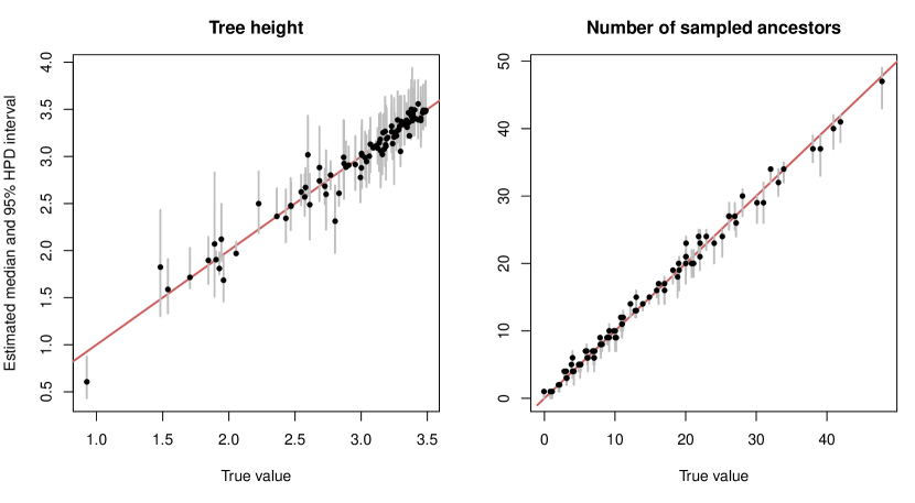
Figure 3: Properties of the tree estimated from simulated data (fossilized birth-death process). The graph shows median estimates (black dots) and 95% HPD intervals (grey lines) against true values for the tree height (on the left) and number of sampled ancestors (on the right).

For the fossilized birth-death process (the process with $\rho$-sampling and zero removal probability), we simulated a set of trees under a fixed set of the tree model parameters. Each parameter was estimated and, in the worst case, the median of the relative errors for all runs was 0.22. The median of the relative errors for tree properties, such as the time of origin, tree height and number of sampled ancestors, was at most 0.09. The true parameters and tree properties were within the estimated 95% HPD intervals at least 95% of the time in all cases. The estimates of the number of sampled ancestors and the tree height are shown in Figure 3. Figure 4 shows how the amount of uncertainty in turnover rate estimates decreases with the size of the tree (i.e., with the number of sampled nodes).

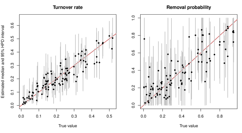
Figure 5: Parameter estimates for simulated data (transmission process). The graph shows median estimates (black dots) and 95% HPD intervals (grey lines) against true values for the turnover rate, $\nu$, (on the left) and removal probability, $r$, (on the right).

To simulate from the transmission birth-death process, i.e., the sampled ancestor birth-death process without $\rho$-sampling and with non-zero removal probability, we draw tree model parameters from uniform distributions for each simulation. The tree model parameters were estimated with the maximum median of relative errors of 0.28 and, for the tree properties, of 0.06. In the worst case a parameter or a tree property was inside the 95% HPD interval 92% of the time. The estimates of the parameters are shown in Figure 5.

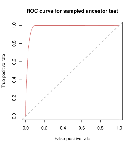
Figure 6: ROC curve for identifying sampled ancestors based on simulated data (transmission process). We identify a node as being a sampled ancestor if the posterior probability that the node is a sampled ancestor is greater than some threshold. The curve is parameterised by the threshold and shows the trade-off between true positive rate (sensitivity) and false positive rate (specificity) (any increase in sensitivity will be accompanied by a decrease in specificity) for different values of the threshold. The dashed diagonal line corresponds to a ‘random guess’ test. The closer the ROC curve to the upper-left boarder of the ROC space (the whole area of the graph), the more accurate the test. The optimal value of the threshold for this curve is 0.45.

We used the data simulated from the transmission process to perform the receiver operating characteristic (ROC) analysis of the sampled ancestor predictor, which makes a prediction relying on the posterior distribution of genealogies. A node is predicted to be a sampled ancestor with a probability calculated as a fraction of trees in the posterior sample in which the node is a sampled ancestor. The total number of non-final sampled nodes (we exclude the most recent node in each case as it can not be a sampled ancestor) in all simulated trees was 5225 and 1814 of these nodes were sampled ancestors. The ROC curve constructed from this data and predictions obtained from the MCMC runs is shown in Figure 6.

Application of the fossilized birth-death model to a bear dataset

In [30], Heath et al. analysed a bear dataset comprised of sequence data of 10 extant species and occurrence dates of 24 fossil samples to estimate divergence times in a Bayesian MCMC framework. They assumed that the tree topology on the extant species is known and each fossil sample is assigned to a clade in the tree. Here, we replicate this analysis using the MCMC implementation of the fossilized birth-death model in BEAST2.

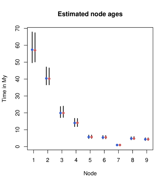
Figure 7: Divergence time estimates for the bear dataset. The estimates are obtained from the analyses with DPPDiv [30] (left bars with blue dots) and BEAST2 (right bars with red dots) implementations of the fossilised birth-death model, which give the same results. The bars are 95% HPD intervals and the dots are mean estimates. The node numbering follows the original analysis [30]: nodes 1 and 2 represent the most recent common ancestors of the bear clade and two outgroups (gray wolf and spotted seal). Node 3 is the most recent common ancestor of all living bear species and nodes 4-9 are the divergence times within the bear clade.

We run two analysis with BEAST2 and with the DPPDiv implementation by Heath et al. under the same model. The tree topology relating all living bear species and two outgroup species is fixed in the analyses and we estimate the divergence times and tree model parameters. The estimates are the same in both analyses as expected. The estimated divergence times are shown in Figure 7.

Application of sampled ancestor Skyline model to HIV dataset

We analysed an HIV-1 subtype B dataset from the United Kingdom, consisting of 62 sequences that were originally analysed in [38] and later analysed using the skyline model without sampled ancestors in [23]. The posterior probability of being a sampled ancestors for three sampled nodes was 61%, 59%, and 49%. For other sampled nodes the probability was less than 4%. There is positive evidence that three sampled nodes with high posterior probabilities are sampled ancestors. The Bayes factors are 5.9, 8.7, and 4.2, respectively.

We chose a random tree among the trees in the posterior sample that have exactly these three nodes as sampled ancestors. The tree is shown in Figure 8. It is noticeable that all three sampled ancestors are clustered on a clade of 16 (out of 62) samples. The median of the posterior distribution of the number of sampled ancestors was 2 with 95% HPD interval $[1,3]$. The removal probability was estimated to be 0.74 with 95% HPD interval $[0.46,0.97]$.

Discussion

The MCMC sampler developed here enables analyses under models in which the probability of one sample being the direct ancestor of another sample is not negligible. These models are useful for describing infectious transmission processes, including identifying transmission chains. They are also useful for estimating divergence times for macroevolutionary data in the presence of fossil samples.

In the analysis of a phylogeny of bears we show that the sampler can be applied to data comprised of both fossil and recent taxa to infer divergence times. This dataset was previously analysed using the fossilized birth-death model by Heath et al. [30]. While the underlying model is the same and thus producing the same results, there is a conceptual difference between the two MCMC frameworks. In the analysis by Heath et al, MCMC was used to integrate over fossil attachment times while the topological attachment of the fossils was integrated out analytically. To achieve this, the topology of the phylogeny relating the extant taxa had to be assumed to be known. In our implementation, we integrate over the trees relating fossil and extant taxa, i.e., over both the fossil attachment times and topological attachment points, using MCMC. In order to facilitate a direct comparison we constrained the topology of the extant species, however the sampler does not require this. For datasets where the tree topology is well resolved, analytical calculation results in faster mixing but when there is uncertainty in the extant phylogeny, which is the more common case, our sampler can account for it. Since the two implementations of the method were made completely independently of one another, this result also provides strong evidence that our implementation is sampling from the correct posterior distribution.

A natural extension to the analysis of the bear phylogeny would be to include morphological data to inform the inference regarding the precise placement of fossils on the tree [32, 33], however this requires models of morphological character evolution [40, 29]. Another direction for application of the sampler is using the skyline version of the fossilized birth-death model to analyse datasets where fossil samples come from different stratigraphic layers, so that rates of fossilisation and discovery may change through time. Fossils are better preserved in some layers than in other layers and therefore the sampling rate varies from layer to layer and this can be modelled as a skyline plot.

Simulation studies show that the MCMC sampler for sampled ancestor trees allows for the detection of direct ancestors within the sample. In epidemiological studies, sampled ancestors can be interpreted as sampled individuals that have later infected other individuals. In the analysis of the HIV dataset, we equated the transmission tree directly with the viral gene tree. This approximation is good enough to demonstrate the method. But for chronic infectious diseases such as Hepatitis C and HIV where the genetic diversity of the pathogen population within a single host can be substantial (e.g. [41, 20]) the inferential power would be improved by a hierarchical model that explicitly models the difference between the sampled ancestor) transmission tree and the (binary) viral gene tree. Regardless of the modelling details, such analyses allow for the estimation of the removal at sampling parameter $r$, which controls the prevalence of sampled ancestors. In most situations this parameter reflects the probability with which patients remain able to cause further infections after they were diagnosed.

Analytic calculations (presented in the Supporting Information) and simulation studies show that there is a degree of non-identifiably of parameters in the transmission birth-death models that include the $r$ parameter. In other words, these models require one of the parameters to be fixed or strongly constrained by prior information to achieve unambiguous inference. In epidemiological studies with a known sampling scheme, a candidate parameter to fix is the sampling proportion. For epidemics with a period of infection, such as influenza, the total removal rate, $\delta$, could be fixed. Under the fossilized birth-death model, it is possible to infer all the parameters of the tree process prior when time-stamped comparative data is available. This is an interesting insight: if no fossils are available, we can only infer two out of the three parameters $\lambda,\mu,\rho$ (as the likelihood only depends on $\lambda-\mu,\lambda\rho$) while in presence of fossils we can estimate all four parameters $\lambda,\mu,\rho,\psi$ (as the likelihood depends on $\lambda-\mu,\lambda\rho,\lambda\psi,\psi$). As sequence data of fossil organisms is rarely available and thus information about fossil locations on the tree obtained by phylogenetic modelling of morphological data [40, 29] may become important to enable effective inference.

To our knowledge this is the first full implementation of an MCMC sampler of sampled ancestor trees and we anticipate that such samplers will form the computational basis for further developments in both fossil-calibrated divergence time dating and phylodynamics.

Figures

Figure 1: Full tree versus reconstructed tree. A full tree produced by the sampled ancestor birth-death process on the left and a reconstructed tree on the right. The sampled nodes are indicated by dots labeled by letters A through H. Nodes A, B and D are sampled ancestors. The reconstructed tree is represented by a sampled ancestor tree $g=(\mathcal{T},(x_{1},x_{2},x_{3},x_{4},y_{1},z_{1},z_{2}))$, where $\mathcal{T}$ denotes the ranked tree topology and $\bar{x}$, $\bar{y}$, and $\bar{z}$ denote the node ages. In the reconstructed tree the root is a sampled node. In the skyline model, birth-death parameters vary from interval to interval. There are two intervals in this figure bounded by the time of origin $t_{0}$, parameter shift time $t_{1}$, and present time $t_{2}$. Between $t_{0}$ and $t_{1}$ parameters $\lambda_{1}$, $\mu_{1}$, $\psi_{1}$ and $r_{1}$ apply and between $t_{1}$ and $t_{2}$ parameters $\lambda_{2}$, $\mu_{2}$, $\psi_{2}$, and $r_{2}$. There are additional sampling attempts at times $t_{1}$ and $t_{2}$ with sampling probabilities $\rho_{1}$ and $\rho_{2}$.

Figure 2: The Wilson Balding operator. The operator proposes a sampled ancestor tree topology and node ages and may propose a tree of larger or smaller dimension (the number of nodes in the tree) than the original tree. First, it prunes a subtree rooted at edge $e_{1}$ (blue edge) either from a branch, coloured black, in case a.1 or from a node, coloured black, in case a.2. Then it attaches the subtree either to an edge $e_{2}$ (black edge) at a random height in case b.1 or to a leaf $l$ (black node) in case b.2. Case a.1 followed by b.2 removes a node from the tree and case a.2 followed by b.1 introduces a new node into the tree.

Figure 4: Uncertainty in estimates for simulated data (fossilized birth-death process). The graph shows the widths of relative 95% HPD intervals of the turnover rate, $\nu$, against tree sizes for simulated fossilized birth-death process.

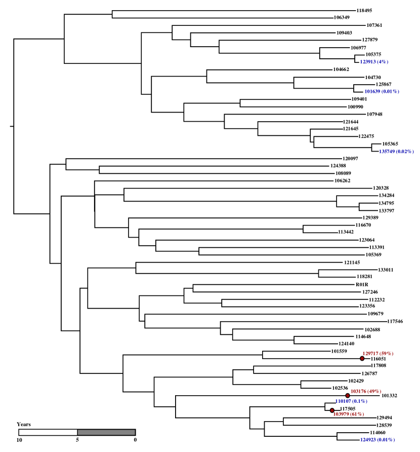
Figure 8: A tree sampled from the posterior of the HIV 1 dataset analysis. The tree exhibits three estimated sampled ancestors shown as red circles. The samples with positive posterior probabilities of being sampled ancestors are shown in colour (red for the nodes with evidence of being sampled ancestors and blue for other nodes with non-zero probabilities) with the posterior probabilities in round brackets.

Tables

Table 1: Hastings ratio for the extension of the Wilson Balding operator

Pruning from /Attaching to	internal branch	leaf	root branch
internal branch	$\frac{|I_{2}|}{|I_{1}|}$	$\frac{D}{(D-1)}\frac{1}{|I_{1}|}$	$\frac{e^{\lambda_{e}h_{2}}}{|I_{1}|}$
internal node	$\frac{D}{(D+1)}|I_{2}|$	$1$	$\frac{D}{(D+1)}e^{\lambda_{e}h_{2}}$
root branch	$\frac{|I_{2}|}{e^{\lambda_{e}h_{1}}}$	$\frac{D}{(D-1)}\frac{1}{e^{\lambda_{e}h_{1}}}$	-

The table summarises the Hastings ratio $\frac{q(g^{*}|g)}{q(g|g^{*})}$ for the extended Wilson Balding operator.

Supporting Information

1 Sampled ancestor Skyline model

Theorem 1.

The probability density function for a reconstructed tree $g=(\mathcal{T},\bar{x},\bar{y},\bar{z})$ produced by the SABD skyline process with parameters $\bar{\lambda},\bar{\mu},\bar{\psi},\bar{r},\bar{\rho},\bar{t}$ is equal to

$$\begin{multlined}f[g|\bar{\lambda},\bar{\mu},\bar{\psi},\bar{r},\bar{\rho},\bar{t}]=\frac{2^{m+M-1}}{(m+M+k+K)!}\times\\ q_{1}(t_{0})\prod_{i=1}^{k}(1-r_{\mathbf{i}_{z_{i}}})\psi_{\mathbf{i}_{z_{i}}}\prod_{i=1}^{m+M-1}\lambda_{\mathbf{i}_{x_{i}}}q_{\mathbf{i}_{x_{i}}}(x_{i})\prod_{i=1}^{m}\frac{\psi_{\mathbf{i}_{y_{i}}}(r_{\mathbf{i}_{y_{i}}}+(1-r_{\mathbf{i}_{y_{i}}})p_{\mathbf{i}_{y_{i}}}(y_{i}))}{q_{\mathbf{i}_{y_{i}}}(y_{i})}\times\\ \prod_{i=1}^{l}((1-\rho_{i})q_{i+1}(t_{i}))^{n_{i}}\rho_{i}^{N_{i}}((1-r_{i+1})q_{i+1}(t_{i}))^{K_{i}}(r_{i+1}+(1-r_{i+1})p_{i+1}(t_{i}))^{M_{i}},\end{multlined}f[g|\bar{\lambda},\bar{\mu},\bar{\psi},\bar{r},\bar{\rho},\bar{t}]=\frac{2^{m+M-1}}{(m+M+k+K)!}\times\\ q_{1}(t_{0})\prod_{i=1}^{k}(1-r_{\mathbf{i}_{z_{i}}})\psi_{\mathbf{i}_{z_{i}}}\prod_{i=1}^{m+M-1}\lambda_{\mathbf{i}_{x_{i}}}q_{\mathbf{i}_{x_{i}}}(x_{i})\prod_{i=1}^{m}\frac{\psi_{\mathbf{i}_{y_{i}}}(r_{\mathbf{i}_{y_{i}}}+(1-r_{\mathbf{i}_{y_{i}}})p_{\mathbf{i}_{y_{i}}}(y_{i}))}{q_{\mathbf{i}_{y_{i}}}(y_{i})}\times\\ \prod_{i=1}^{l}((1-\rho_{i})q_{i+1}(t_{i}))^{n_{i}}\rho_{i}^{N_{i}}((1-r_{i+1})q_{i+1}(t_{i}))^{K_{i}}(r_{i+1}+(1-r_{i+1})p_{i+1}(t_{i}))^{M_{i}},$$ (9)

where, for $i=1,\ldots,l$ and $t_{i}\leq t<t_{i-1}$,

$$p_{i}(t)=\frac{\lambda_{i}+\mu_{i}+\psi_{i}-A_{i}\frac{e^{A_{i}(t-t_{i})}(1+B_{i})-(1-B_{i})}{e^{A_{i}(t-t_{i})}(1+B_{i})+(1-B_{i})}}{2\lambda_{i}}$$

with

$$A_{i}=\sqrt{(\lambda_{i}-\mu_{i}-\psi_{i})^{2}+4\lambda_{i}\psi_{i}}$$

and

$$B_{i}=\frac{(1-2(1-\rho_{i})p_{i+1}(t_{i}))\lambda_{i}+\mu_{i}+\psi_{i}}{A_{i}};$$

$p_{l+1}(t_{l})=1$; and, for $i=1,\ldots,l$,

$$q_{i}(t)=\frac{4e^{A_{i}(t-t_{i})}}{(e^{A_{i}(t-t_{i})}(1+B_{i})+(1-B_{i}))^{2}}.$$

The other notation is summarised in table 2

Table 2: Sampled ancestor Skyline model notation

Notation	Description
$l$	the number of intervals or parameter shift times,
$t_{or}$	$t_{or}=t_{0}$ the time of origin,
$t_{i}$	is parameter shift time or $\rho$-sampling time for $i\in\{1,\ldots,l\}$ with $t_{l}=0$,
$\bar{t}$	$(t_{0},\ldots,t_{l-1})$ is a vector of those time parameters which are necessary to define the model,
$m$	the number of $\psi$-sampled tips,
$\bar{y}$	$(y_{1},\ldots,y_{m})$ is a vector of times of $\psi$-sampled tips,
$M_{i}$	the number of tips sampled at time $t_{i}$ for $i\in\{1,\ldots,l\}$,
$M$	$\sum\limits_{i=1}^{l}M_{i}$,
$\bar{x}$	$(x_{1},\ldots,x_{m+M})$ is a vector of bifurcation times,
$k$	the number of $\psi$-sampled nodes that have sampled descendants,
$\bar{z}$	$(z_{1},\ldots,z_{k})$ is a vector of times of $\psi$-sampled nodes with sampled descendants,
$K_{i}$	the number of nodes, with sampled descendants, sampled at time $t_{i}$ for $i\in\{1,\ldots,m\}$
$K$	$\sum\limits_{i=1}^{l}K_{i}$,
$N_{i}$	$K_{i}+M_{i}$ the total number of nodes sampled at time $t_{i}$ for $i\in\{1,\ldots,l\}$,
$n_{i}$	the number of lineages presented in the tree at time $t_{i}$ but not sampled at this time for $i~{}\in~{}\{1,\ldots,l\}$,
${\bf i}_{x}$	an index such that $t_{{\bf i}_{x}}\leq x<t_{{\bf i}_{x}-1}$.

Proof.

First, we consider the same process but where at each bifurcation time, we label one of the new lineages as left and another as right and we do not label sampled nodes. In this case, the process produces oriented trees instead of labeled trees.

The probability $p_{i}(t)$ that an individual alive at time $t$ has no sampled descendants when the process is stopped (i.e., in the time interval $[t_{l},t]$), with $t_{i}\leq t<t_{i-1}$ ($i=1,\ldots,l$) was derived in [23] for the birth-death skyline model without sampled ancestor (i.e. $r=1$).

Consider an event that the individual that started the process at time $t_{or}$ has no sampled descendants in the time interval $[t_{l},t_{or}]$. This event does not depend on the behaviour of the process if an individual was sampled (such as the possibility to remain in the process after sampling, i.e., $r<1$) because it states that no individual was sampled. That implies $p_{1}(t_{or}|\lambda,\mu,\psi,r)=p_{1}(t_{or}|\lambda,\mu,\psi)$. Since the evolution of each lineage is independent of the evolution of other coexisting lineages under this model, we can state the same for the event that an individual alive at some time $t<t_{or}$ has no sampled descendant when the process is stopped, that is, $p_{i}(t|\lambda,\mu,\psi,r)=p_{i}(t|\lambda,\mu,\psi)$ for $i$ as above.

For convenience, we split every edge existing at time $t_{i}$ (for $i=1,\ldots,l-1$) with a two degree node dated at this time. Let $g_{i,e}(t)$ be the probability density that an infected individual in the tree at time $t$ corresponding to edge $e$ (with $t_{i}\leq t\leq t_{i-1}$) evolved between $t$ and the present as observed in the tree.

The Master equation for $g_{i,e}(t)$ along an edge with starting time $t_{s}$ and ending time $t_{b}$ ($t_{e}\leq t\leq t_{b}$) is

$$\frac{d}{dt}g_{i,e}(t)=-(\lambda_{i}+\mu_{i}+\psi_{i})g_{i,e}(t)+2\lambda_{i}p_{i}(t)g_{i,e}(t)$$

Note that $r$ does not occur in the equation and will only be introduced in the initial values of $g_{i,e}$. The solution to this equation is given in [23]:

$$g_{i,e}(t)=g_{i,e}(t_{e})\frac{q_{i}(t)}{q_{i}(t_{e})}.$$

Further, the initial values are, for $t_{e}\neq t_{i}$,

$$g_{i,e}(t_{e})=\begin{cases}\lambda_{i}g_{i,e_{1}}(t_{e})g_{i,e_{2}}(t_{e})&\text{ if $e$ has two descendant edges $e_{1}$, $e_{2}$,}\\ \psi_{i}(r_{i}+(1-r_{i})p_{i}(t_{e}))&\text{ if $e$ is a leaf edge, }\\ \psi_{i}(1-r_{i})g_{i,e_{1}}(t_{e})&\text{ if $e$ has one descendant edge $e_{1}$;}\\ \end{cases}$$

and for $t_{e}=t_{i}$,

$$g_{i,e}(t_{e})=\begin{cases}(1-\rho_{i})g_{i+1,e_{1}}(t_{e})&\parbox[t]{172.99496pt}{if $e$ has one descendant edge $e_{1}$ and $e$ is not a sampled node,}\\ \rho_{i}(1-r_{i+1})g_{i+1,e_{1}}(t_{e})&\parbox[t]{172.99496pt}{if $e$ has one descendant edge $e_{1}$ and $e$ is a sampled node,}\\ \rho_{i}(r_{i+1}+(1-r_{i+1})p_{i+1}(t_{e}))&\text{if $e$ is a leaf edge;}\\ \end{cases}$$

Then the probability density of the genealogy is

$$f[g|\bar{\lambda},\bar{\mu},\bar{\psi},\bar{r},\bar{\rho},\bar{t}]=g_{1,e_{root}}(t_{0})$$

Traversing the tree from tips to the root and finding $g_{i,e}(t_{e})$ for each time $t_{e}$ (note that $q_{i}(t_{i})=1$), we derive that $g_{1,e_{root}}(t_{0})$ is as in (9) without the first term, which comes from the fact that we considered oriented trees instead of labeled trees.

Indeed, the expression without the first term is the probability density function for oriented trees. Having the model parameters fixed (including $\bar{t}$), it only depends on branching times, sampling times of tips, sampling times of two degree nodes, the number of sampled two-degree nodes at time $t_{i}$, and the number of sampled tips at time $t_{i}$ (i.e., on $\bar{x}$, $\bar{y}$, $\bar{z}$, $\bar{K}$, and $\bar{M}$), but not on how the lineages are connected, i.e. not on the particular topology. The density of an oriented and labeled genealogy which has the given oriented tree embedded is the oriented tree probability divided by the $(m+M+k+K)!$ possible labelings. Ignoring the $2^{m+M-1}$ orientations establishes the theorem. ∎

Re-parameterisation

Let $\rho_{1},\ldots,\rho_{l-1}=0$ and consider the re-parameterisation, collapsing the original $4l+1$ parameters into $4l$ parameters:

$$d_{i}=\lambda_{i}-\mu_{i}-\psi_{i} \text{ for }i=1,\ldots,l$$ (10)

$$f_{i}=\lambda_{i}\psi_{i} \text{ for }i=1,\ldots,l$$

$$g_{i}=(1-r_{i})\psi_{i} \text{ for }i=1,\ldots,l$$

$$h=\rho_{l}\lambda_{l}$$

$$k_{i}=\frac{\lambda_{i}}{\lambda_{i+1}} \text{ for }i=1,\ldots,l-1$$

We will show in the following that the tree likelihood derived in Theorem 1 conditioned on $\psi$-sampling at least one individual and with $\rho_{1},\ldots,\rho_{l-1}=0$ depends only on the $4l$ parameters obtained from the re-parameterisation, thus in the original parameter set of size $4l+1$, one parameter cannot be identified from the sampled tree.

Lemma 1.

Let $\zeta_{i}(t)=A_{i}\frac{e^{A_{i}(t-t_{i})}(1+B_{i})-(1-B_{i})}{e^{A_{i}(t-t_{i})}(1+B_{i})+(1-B_{i})}$. Then

$$A_{i}=\sqrt{d_{i}^{2}+4f_{i}} \text{ for }i =1,\ldots,l;$$

$$B_{i}=\frac{k_{i}(d_{i+1}+\zeta_{i+1}(t_{i}))-d_{i}}{A_{i+1}} \text{ for }i =1,\ldots,l-1;$$

$$B_{l}=\frac{2h-d_{l}}{A_{l}};$$

$$r_{i}+(1-r_{i})p_{i}(t)=\frac{g_{i}}{2f_{i}}\Bigl{(}\frac{2f_{i}}{g_{i}}-d_{i}-\zeta_{i}(t)\Bigr{)} \text{ for }i =1,\ldots,l;\text{ and}$$

$$1-p_{i+1}(t)=\frac{d_{i+1}+\zeta_{i+1}(t)}{2\lambda_{i+1}} \text{ for }i =0,\ldots,l-1.$$

Proof.

We show only one case:

$$r_{i}+(1-r_{i})p_{i}(t)=r_{i}+(1-r_{i})\frac{\lambda_{i}+\mu_{i}+\psi_{i}-\zeta_{i}(t)}{2\lambda_{i}}=$$

$$\frac{(1-r_{i})}{2\lambda_{i}}\Bigl{(}\frac{2\lambda_{i}r_{i}}{(1-r_{i})}+\lambda_{i}+\mu_{i}+\psi_{i}-\zeta_{i}(t)\Bigr{)}=$$

$$\frac{g_{i}}{2f_{i}}\Bigl{(}\frac{2\lambda_{i}}{(1-r_{i})}-2\lambda_{i}+\lambda_{i}+\mu_{i}+\psi_{i}-\zeta_{i}(t)\Bigr{)}=\frac{g_{i}}{2f_{i}}\Bigl{(}\frac{2f_{i}}{g_{i}}-d_{i}-\zeta_{i}(t)\Bigr{)}$$

Other equations can be verified by substituting parameters $\bar{d}$, $\bar{f}$, $h$, and $\bar{k}$ with expressions given in (10).

∎

Theorem 2.

When $\rho_{1},\ldots,\rho_{l-1}=0$, the tree density function for the sampled ancestor model conditioned on $\psi$-sampling at least one individual, which is

$$f[g|\bar{\lambda},\bar{\mu},\bar{\psi},\bar{r},\rho_{l},\bar{t},S]\propto$$

$$\rho_{l}^{N_{l}}\frac{q_{1}(t_{0})}{1-p_{1}(t_{0})}\prod_{i=1}^{k}(1-r_{\mathbf{i}_{z_{i}}})\psi_{\mathbf{i}_{z_{i}}}\prod_{i=1}^{m+N_{l}-1}2\lambda_{\mathbf{i}_{x_{i}}}q_{\mathbf{i}_{x_{i}}}(x_{i})\prod_{i=1}^{m}\frac{\psi_{\mathbf{i}_{y_{i}}}(r_{\mathbf{i}_{y_{i}}}+(1-r_{\mathbf{i}_{y_{i}}})p_{\mathbf{i}_{y_{i}}}(y_{i}))}{q_{\mathbf{i}_{y_{i}}}(y_{i})}\prod_{i=1}^{l}(q_{i+1}(t_{i}))^{n_{i}}$$

can be re-parameterised with parameters given in Equations (10).

Proof.

We can write this function as follows:

$$\rho_{l}^{N_{l}}\lambda_{1}\prod_{i=1}^{m+N_{l}-1}\lambda_{\mathbf{i}_{x_{i}}}\prod_{i=1}^{m}\psi_{\mathbf{i}_{y_{i}}}\times$$

$$\frac{q_{1}(t_{0})}{\lambda_{1}(1-p_{1}(t_{0}))}\prod_{i=1}^{k}(1-r_{\mathbf{i}_{z_{i}}})\psi_{\mathbf{i}_{z_{i}}}\prod_{i=1}^{m+N_{l}-1}2q_{\mathbf{i}_{x_{i}}}(x_{i})\prod_{i=1}^{m}\frac{(r_{\mathbf{i}_{y_{i}}}+(1-r_{\mathbf{i}_{y_{i}}})p_{\mathbf{i}_{y_{i}}}(y_{i}))}{q_{\mathbf{i}_{y_{i}}}(y_{i})}\prod_{i=1}^{l}(q_{i+1}(t_{i}))^{n_{i}}$$

From lemma 1, it follows that $q_{i}(t)$, $\lambda_{1}(1-p_{1}(t_{0}))$, $r_{i}+(1-r_{i})p_{i}(t)$ depend only on parameters $\bar{d}$, $\bar{f}$, $\bar{g}$, $h$ and $\bar{k}$ and do not depend on $\bar{\lambda}$, $\bar{\mu}$, $\bar{\psi}$, $\bar{r}$, $\rho_{l}$ individually. It remains to show that

$$\rho_{l}^{N_{l}}\lambda_{1}\prod_{i=1}^{m+N_{l}-1}\lambda_{\mathbf{i}_{x_{i}}}\prod_{i=1}^{m}\psi_{\mathbf{i}_{y_{i}}}$$

also depends only on $\bar{d}$, $\bar{f}$, $\bar{g}$, $h$ and $\bar{k}$.

Note that

$$\psi_{i}\lambda_{j}=f_{i}k_{i}\ldots k_{i} \text{ for }j<i,$$

$$\rho_{l}\lambda_{i}=hk_{i}\ldots k_{l} \text{ for }j<l.$$

and we can decompose the last term in $m+N_{l}$ terms in either of the two forms: $\psi_{i}\lambda_{j}$ and $\psi_{l}\lambda_{i}$. ∎

Setting $\rho_{l}$ to zero in re-parameterisation (10), we can see that function (4) depends on $4l-1$ parameters: $\bar{d}$, $\bar{f}$, $\bar{g}$ and $k_{1},\ldots,k_{l-1}$, out of $4l$ parameters: $\bar{\lambda}$, $\bar{\mu}$, $\bar{\psi}$ and $\bar{r}$. Also, setting $l=1$, $\lambda_{1}=\lambda$, $\mu_{1}=\mu$, $\psi_{1}=\psi$, and $r_{1}=r$ gives us that $p_{1}(t)=p_{0}(t)$ and $q_{1}(t)=q(t)$ and that $f[g|\lambda,\mu,\psi,r,t_{0},S]$ is basically the same function as in (1). That means that we can re-parameterise function (1) with $\lambda-\mu-\psi$, $\lambda\psi$ and $\psi(1-r)$.

In a similar manner, we can show that when $\bar{r}=0$, $\rho_{l}\neq 0$ and conditioning on sampling at least one extant individual (i.e., considering skyline fossilised birth-death process with tree probability density (5)), function $\lambda_{1}(1-\hat{p}_{1}(t))=\lambda_{1}(1-p_{1}(t|\bar{\psi}=0))$ depends on

$$\hat{d}_{i}=\lambda_{i}-\mu_{i} \text{ for }i =1,\ldots,l;$$

$$k_{i}=\frac{\lambda_{i}}{\lambda_{i+1}} \text{ for }i =1,\ldots,l-1;\text{ and}$$

$$h=\rho_{l}\lambda_{l}.$$

Note that $\hat{d}_{i}=d_{i}-g_{i}$ because $r_{i}=0$ implying $g_{i}=\psi_{i}$ for all $i$. That means we can re-parameterise (5) with (10). But for this model, we have $3l+1$ initial parameters: $\bar{\lambda}$, $\bar{\mu}$, $\bar{\psi}$, and $\rho_{l}$, and $4l$ new parameters: $\bar{d}$, $\bar{f}$, $\bar{g}$, $k_{1},\ldots,k_{l-1}$ and $h$; implying that re-parameterisation (10) does not reduce the number of parameters in function (5).

2 Testing Operators

We introduced a number of operators for a random walk in the space of sampled ancestor trees and implemented the operators as a sampled ancestor add-on to the BEAST2 software. To test the implementation we run the MCMC sampler to obtain a sample from the tree distribution defined by the sampled ancestor birth-death model [15] and compare the results with calculations made in Mathematica software.

The probability density of the tree distribution is

$$f[g|\lambda,\mu,\psi,r,t_{or}]=\frac{1}{(k+m)!}q(t_{or})(\psi(1-r))^{k}\prod_{i=1}^{m-1}2\lambda q(x_{i})\prod_{i=1}^{m}\frac{\psi(r+(1-r)p_{0}(y_{i}))}{q(y_{i})}$$

We fix sample size $n=k+m$, sampling dates $\bar{y}$ and all the model parameters except for the time of origin $t_{or}$ placing a uniform distribution on it. So we sample genealogies from the distribution with probability density:

$$f[g,t_{or}|\lambda,\mu,\psi,r;n,\bar{y}]=f[g|\lambda,\mu,\psi,r,t_{or};n,\bar{y}]f_{or}(t_{or})$$ (11)

where $f_{or}(x)$ is a probability density of the origin. We set,

$\lambda=2$	$\mu=1$	$\psi=0.5$	$r=0.9$
$t_{or}\sim$ Uniform(0, 1000)
$n=3$	$y_{1}=2$	$y_{2}=1$	$y_{3}=0$

We run 100 MCMC analysis to test different operators that do not change sampled node’s times.

To assess whether the obtained tree samples are from distribution (11) with the given parameters we calculate the true marginal probabilities for all non-ranked tree topologies on three sequentially sampled individuals in Mathematica. There are eight different non-ranked tree topologies. Denote them $T_{1},\ldots,T_{8}$. To fix string representations for the topologies we label the individual sampled at time $y_{1}$ as $1$, at time $y_{2}$ as $2$, and at time $y_{3}$ as $3$. The true probabilities are shown in the table below:

Non-ranked tree topology	String representation	Probability in %
$T_{1}$	$((3,2),1)$	$77.8327$
$T_{2}$	$((3,2))1$	$7.8642$
$T_{3}$	$((3)2,1)$	$3.8657$
$T_{4}$	$(3,(2,1))$	$4.3189$
$T_{5}$	$((3,1),2)$	$4.3189$
$T_{6}$	$((3)2)1$	$0.4135$
$T_{7}$	$(3,(2)1)$	$0.6930$
$T_{8}$	$((3)1,2)$	$0.6930$

Further we compare the estimated marginal probabilities with the true marginal probabilities. We calculate the standard errors of the estimated probabilities for each tree topology and assess if the estimated value is within two standard errors of the true value. To calculate a standard error given by:

$$\frac{p_{true}(1-p_{true})}{\sqrt{ESS}}$$

we need to find the number of independent samples, i.e. the effective sample size (ESS). To find the ESS we assign an integer to each of the eight topologies to obtain a sample from $\{1,\ldots,8\}$ instead of a tree sample and calculate the ESS for the integer sample.

The obtained results for 100 runs are summarised in the following table:

Operators	Accuracy for non-ranked tree topologies (in %)
	$T_{1}$	$T_{2}$	$T_{3}$	$T_{4}$	$T_{5}$	$T_{6}$	$T_{7}$	$T_{8}$
WB	96	96	99	95	96	98	95	95
WB	98	95	94	92	93	96	96	98
WB and S	97	95	97	98	97	98	99	97
WB, LSJ, and Ex	92	97	97	99	98	98	95	96
WB, LSJ, Ex, and S	95	94	96	98	93	92	99	98
WB, LSJ, Ex, U, and S	94	93	91	97	93	92	94	95

3 Simulation studies

We divide the simulations in two groups. In one group of simulations (Scenario 1), we simulate trees and then estimate tree model parameters with the trees fixed in MCMC. In the second type of simulations (Scenario 2), we simulate trees and sequences along the simulated trees and then run MCMC with sequences and sampled node dates as the input data to estimate tree model parameters, trees, and molecular model parameters.

We simulate 100 trees in all the scenarios except for the last scenario of the skyline model simulations. When simulating trees, we either fix a set of tree model parameters and simulate each tree under the model with the fixed parameters or draw a new set of parameters from prior distributions for each tree. Further we either simulate the process until it reaches a pre-defined number of sampled nodes or until a pre-defined time length (the time of origin) is reached.

For models without $\rho$-sampling, we fix one of the parameters to its true value in MCMC (as not all parameters can be inferred). In all scenarios, we place a uniform prior on $[0,1000]$ for the time of origin.

We simulate sequences of 2000 bp under the GTR model with fixed rates and frequencies:

$$(\eta_{AC},\eta_{AG},\eta_{AT},\eta_{CG},\eta_{CT},\eta_{GT})=(0.4,1.0,0.1,0.15,1.04,0.15)$$

$$(\pi_{A},\pi_{C},\pi_{G},\pi_{T})=(0.25,0.25,0.25,0.25)$$

We use the strict molecular clock model with a fixed substitution rate.

For each estimated parameter, we take the median of its posterior distribution as a point estimate. We calculate the error and relative bias of the median estimate and relative 95% high probability density (HPD) interval width. And we assess whether the true value is inside the 95% HPD interval.

$$error=\frac{|true~{}value-median|}{true~{}value}$$

$$relative~{}bias=\frac{true~{}value-median}{true~{}value}$$

$$relative~{}95\%HPD~{}width=\frac{upper-lower}{true~{}value}$$

where $upper$ and $lower$ are the upper and lower bounds of the 95% HPD interval.

Then we summarise the statistics from 100 runs and report medians of 100 errors, 100 relative biases, and 100 relative 95% HPD width. We also report the 95% HPD accuracy, which is the number of times when the true value was inside the 95% HPD interval.

Simulation of the sampled ancestor birth-death model

Scenario 1

In scenarios 1.1, 1.2, and 1.4, we simulate under the model without $\rho$-sampling, i.e., $\rho=0$. In Scenarios 1.1 and 1.2, parameters are fixed and we stop simulations when a sample of 200 is reached. In Scenario 1.3, we simulate trees on a fixed time interval of $t_{or}$. We discard trees with too small or too large numbers of sampled nodes. In Scenario 1.4, we draw parameters $\lambda$, $\mu$, $\psi$, and $r$ from uniform prior distributions and simulate trees with 100 sampled nodes.

	true value	prior	median	error	relative bias	relative 95% HPD width	95% HPD accuracy in %
Scenario 1.1: $\psi$ fixed in MCMC.
$\lambda$	0.9	U(0,100)	0.9222	0.0735	0.0247	0.4056	96
$\mu$	0.2	U(0,100)	0.2219	0.3885	0.1096	2.2460	94
$\psi$ (fixed)	0.3	-	-	-	-	-	-
$r$	0.6	U(0,1)	0.5823	0.0880	-0.0295	0.4087	93
Scenario 1.2: $r$ fixed in MCMC.
$\lambda$	1.0	U(0,100)	1.0861	0.0921	0.0861	0.5020	96
$\mu$	0.1	U(0,100)	0.1871	0.8705	0.8705	4.8774	98
$\psi$	0.4	U(0,100)	0.3841	0.0888	-0.0399	0.4821	93
$r$ (fixed)	0.5	-	-	-	-	-	-
Scenario 1.3: $r=0$ and simulations stop at $t_{or}$.
$t_{or}$	5.0	U(0,1000)	4.8545	0.0815	-0.0291	0.4509	97
$\lambda$	1.5	U(0,100)	1.6077	0.1112	0.0718	0.7094	93
$\mu$	0.5	U(0,100)	0.6494	0.4088	0.2988	2.1971	94
$\psi$	0.2	U(0,100)	0.1884	0.1840	-0.0579	0.8871	90
$\rho$	0.8	U(0,1)	0.7756	0.0916	-0.0305	0.5446	97
Scenario 1.4: parameters drawn from priors.
$\lambda$	-	U(1,1.5)	1.2899	0.0640	-0.0106	0.3324	95
$\mu$	-	U(0.5, 1)	0.6727	0.1546	0.0321	0.6520	92
$\psi$ (fixed)	-	U(4,5)	-	-	-	-	-
$r$	-	U(0,1)	0.0499	0.4630	-0.0853	2.0262	92

Scenario 2

In Scenarios 2.1.1 and 2.1.2, we use the model without $\rho$-sampling and stop simulations when a sample of 200 is reached. The tree model parameters are fixed. In Scenarios 2.2 and 2.3, we use $d$, $r_{t}$, and $s$ parameterisation, i.e., we estimate and place priors on parameters

$d=\lambda-\mu$

$r_{t}=\frac{\mu}{\lambda}$

$s=\frac{\psi}{\mu+\psi}$

instead of $\lambda$, $\mu$ and $\psi$.

In Scenario 2.2, we set $r=0$ and stop simulations when time $t_{or}=3.5$ reached. The average number of sampled nodes is 50. We discard trees with less than 5 sampled nodes, and analyse 92 remaining trees.

In Scenario 2.3, the tree model parameters drawn from the prior distributions. The stop simulation condition is when the time of origin reaches $3.0$. We discard trees with less than 5 or more than 250 sampled nodes, which constitutes in total 21% of simulated trees. The average number of sampled nodes in remaining trees is 53. $s$ is fixed in MCMC.

	true value	prior	median	error	relative bias	relative 95% HPD width	95% HPD accuracy in %
Scenario 2.1.1: $\mu_{s}=0.02$
$t_{or}$	-	U(0,1000)	-	0.0347	0.0066	0.2398	95
Tree height	-	SABD	-	0.0065	-1e05	0.0404	97
# SA	-	SABD	-	0.0714	0.0000	0.3043	97
$\lambda$	1.0	U(0,100)	1.0486	0.0825	0.0486	0.4231	93
$\mu$	0.2	U(0, 100)	0.2456	0.3436	0.2279	2.5473	95
$\psi$ (fixed)	0.4	-	-	-	-	-	-
$r$	0.7	U(0,1)	0.6753	0.057	-0.0353	0.3301	93
Scenario 2.1.2: $\mu_{s}=0.0002$
$t_{or}$	-	U(0,1000)	-	0.0504	0.0009	0.2856	94
Tree height	-	SABD	-	0.0221	-0.0067	0.1423	96
# SA	-	SABD	-	0.3784	0.2660	1.9307	98
$\lambda$	1.0	U(0,100)	1.1206	0.1343	0.1206	0.7940	95
$\mu$	0.2	U(0,100)	0.3397	0.6984	0.6984	4.0758	95
$\psi$ (fixed)	0.4	-	-	-	-	-	-
$r$	0.7	U(0,1)	0.5726	0.1915	-0.1820	1.0405	93

	true value	prior	median	error	relative bias	relative 95% HPD width	95% HPD accuracy in %
Scenario 2.2: $r=0$ and simulations stop at $t_{or}$
$t_{or}$	3.5	U(0,1000)	3.5776	0.0857	0.0222	0.5816	96
Tree height	-	SABD	-	0.0170	0.0000	0.1480	95
# SA	-	SABD	-	0.0241	0.0000	0.1905	99
$\mu_{s}$	0.01	ln$\mathcal{N}$(-4.6, 1.25)	0.0099	0.0342	-0.0076	0.2304	95
$d$	1.0	U(0,1000)	1.0266	0.1872	0.0266	1.0317	95
$r_{t}$	0.3333	U(0,1)	0.3343	0.2236	0.0029	1.7816	100
$s$	0.4444	U(0,1)	0.4343	0.1844	-0.0229	1.2984	98
$\rho$	0.7	U(0,1)	0.6854	0.1116	-0.0209	0.8005	95
Scenario 2.3: $\rho=0$, parameters drawn from priors and simulations stop at $t_{or}$
$t_{or}$	3.0	U(0,1000)	3.0084	0.05096	0.0157	0.4301	98
Tree height	-	SABD	-	0.0168	-1e-07	0.1322	94
# SA	-	SABD	-	0.0493	0.0000	0.3636	98
$\mu_{s}$	0.01	ln$\mathcal{N}$(-4.6, 1.25)	0.0100	0.0550	0.0023	0.2515	93
$d$	-	U(1,2)	1.5217	0.1053	0.0023	0.5239	93
$r_{t}$	-	U(0,1)	0.1956	0.2084	0.0037	0.8309	95
$r$	-	U(0,1)	0.3146	0.2814	-0.0065	1.3304	92
$s$ (fixed)	-	U(0.5, 1)	-	-	-	-

Simulation of the sampled ancestor skyline model

In all three scenarios for simulation of the skyline model, we simulate the process until a sample of 200 is reached. We only simulate trees and do not simulate sequences in these scenarios. In Scenario 1.1, there are two intervals and only sampling rate shifts from zero to non-zero value. In Scenario 1.2, there are two intervals and all parameters except $r$, which is fixed in the MCMC, shifts at time $t_{1}=5.0$. In Scenario 1.3, we have three intervals with the shift times: $t_{1}=3.0$ and $t_{2}=6.0$. All parameters shift. All elements of vector $\bar{r}$ are fixed in MCMC. In this last scenario, we simulated 50 trees and present the results on 42 successful MCMC runs (other runs did not converge with the chain length of 20M states).

	true value	prior	median	error	relative bias	relative 95% HPD width	95% HPD accuracy in %
Scenario 1.1: two intervals and only $\psi$ shifts from zero to non-zero value.
$\lambda$	0.8	U(0,100)	0.8107	0.0861	0.0134	0.4577	92
$\mu$	0.4	U(0,100)	0.4199	0.2070	0.0499	1.1330	94
$\psi$ (fixed)	0.2	-	-	-	-	-	-
$r$	0.8	Uniform(0,1)	0.7874	0.0394	-0.0158	0.2516	97
Scenario 1.2: two intervals and all parameters except $r$ shift.
$\lambda_{1}$	1.0	U(0, 100)	1.1869	0.2072	0.1869	1.1345	100
$\lambda_{2}$	0.8	U(0, 100)	0.8442	0.065	0.0552	0.6402	100
$\mu_{1}$	0.2	U(0, 100)	0.3660	0.8298	0.8298	6.0261	100
$\mu_{2}$	0.2	U(0, 100)	0.2640	0.4035	0.3200	3.1496	100
$\psi_{1}$	0.4	U(0, 100)	0.3452	0.2056	-0.1371	0.9341	94
$\psi_{2}$	0.5	U(0, 100)	0.4847	0.0915	-0.0305	0.5592	96
$r$ (fixed)	0.7	-	-	-	-	-	-
Scenario 1.3: three intervals, all parameters shift and vector $\bar{r}$ fixed.
$\lambda_{1}$	1.5	U(0, 100)	1.6988	0.2385	0.1325	1.2336	95
$\lambda_{2}$	1.2	U(0, 100)	1.3945	0.2014	0.1621	0.8813	95
$\lambda_{3}$	0.5	U(0, 100)	0.5480	0.1568	0.0960	1.2625	100
$\mu_{1}$	0.5	U(0, 100)	0.7108	0.5132	0.4216	3.5732	100
$\mu_{2}$	0.6	U(0, 100)	0.8086	0.4067	0.3477	1.9862	90
$\mu_{3}$	0.2	U(0, 100)	0.2594	0.4856	0.2968	3.2805	100
$\psi_{1}$	0.4	U(0, 100)	0.4057	0.2359	0.0141	1.2262	90
$\psi_{2}$	0.5	U(0, 100)	0.4497	0.1706	-0.1006	0.6650	90
$\psi_{3}$	0.1	U(0, 100)	0.0967	0.1933	-0.0327	1.0046	98
$r_{1}$ (fixed)	0.1	-	-	-	-	-	-
$r_{2}$ (fixed)	0.5	-	-	-	-	-	-
$r_{3}$ (fixed)	0.9	-	-	-	-	-	-

4 HIV-1 data analysis

For some of the taxon names in the tree in Figure 8M the accession numbers are given in the table.

taxon name	accession number	taxon name	accession number
129717	AY362152.1	103979	AY362145.1
126787	AY362151.1	134795	AY362101.1
102429	AY362149.1	134284	AY362100.1
103176	AY362148.1	101559	AY362057.1
124923	AY362147.1	102536	AY362056.1
117505	AY362146.1	RO1R	AF494119.1

References

- 1. Yang Z, Rannala B (1997) Bayesian phylogenetic inference using DNA sequences: a Markov chain Monte Carlo method. Mol Biol Evol 14: 717-24.
- 2. Mau B, Newton MA, Larget B (1999) Bayesian phylogenetic inference via Markov chain Monte Carlo methods. Biometrics 55: 1-12.
- 3. Huelsenbeck JP, Ronquist F (2001) MRBAYES: Bayesian inference of phylogenetic trees. Bioinformatics 17: 754-5.
- 4. Drummond AJ, Suchard MA, Xie D, Rambaut A (2012) Bayesian phylogenetics with BEAUti and the BEAST 1.7. Mol Biol Evol 29: 1969-73.
- 5. Ronquist F, Teslenko M, van der Mark P, Ayres DL, Darling A, et al. (2012) MrBayes 3.2: efficient Bayesian phylogenetic inference and model choice across a large model space. Syst Biol 61: 539–42.
- 6. Bouckaert R, Heled J, Künert D, Vaughan TG, Wu CH, et al. (2014) BEAST2: A software platform for Bayesian evolutionary analysis. PLoS Comput Biol 10: e1003537.
- 7. Lartillot N, Lepage T, Blanquart S (2009) PhyloBayes 3: a Bayesian software package for phylogenetic reconstruction and molecular dating. Bioinformatics 25: 2286-8.
- 8. Metropolis N, Rosenbluth A, Rosenbluth M, Teller A, Teller E (1953) Equations of state calculations by fast computing machines. Journal of Chemistry and Physics 21: 1087–1092.
- 9. Hastings W (1970) Monte Carlo sampling methods using Markov chains and their applications. Biometrika 57: 97–109.
- 10. Lewis PO, Holder MT, Holsinger KE (2005) Polytomies and Bayesian phylogenetic inference. Syst Biol 54: 241–253.
- 11. Gavryushkina A, Welch D, Drummond AJ (2013) Recursive algorithms for phylogenetic tree counting. Algorithms for Molecular Biology 8: 26.
- 12. Drummond A, Pybus O, Rambaut A, Forsberg R, Rodrigo A (2003) Measurably evolving populations. Trends in Ecology & Evolution 18: 481–488.
- 13. Pybus OG, Charleston MA, Gupta S, Rambaut A, Holmes EC, et al. (2001) The epidemic behavior of the hepatitis C virus. Science 292: 2323-2325.
- 14. Grenfell BT, Pybus OG, Gog JR, Wood JLN, Daly JM, et al. (2004) Unifying the epidemiological and evolutionary dynamics of pathogens. Science 303: 327-32.
- 15. Stadler T, Kouyos RD, von Wyl V, Yerly S, Böni J, et al. (2011) Estimating the basic reproductive number from viral sequence data. Molecular Biology and Evolution 29: 347-357.
- 16. Ypma RJ, van Ballegooijen WM, Wallinga J (2013) Relating phylogenetic trees to transmission trees of infectious disease outbreaks. Genetics 195: 1055-1062.
- 17. Künert D, Stadler T, Vaughan TG, Drummond AJ (2014) Simultaneous reconstruction of evolutionary history and epidemiological dynamics from viral sequences with the birth-death SIR model. J R Soc Interface 11: 20131106.
- 18. Volz EM, Frost SD (2013) Inferring the source of transmission with phylogenetic data. PLoS computational biology 9: e1003397.
- 19. Teunis P, Heijne JCM, Sukhrie F, van Eijkeren J, Koopmans M, et al. (2013) Infectious disease transmission as a forensic problem: who infected whom? J R Soc Interface 10: 20120955.
- 20. Vrancken B, Rambaut A, Suchard MA, Drummond A, Baele G, et al. (2014) The genealogical population dynamics of HIV-1 in a large transmission chain: Bridging within and among host evolutionary rates. PLoS Comput Biol 10: e1003505.
- 21. Stadler T (2010) Sampling-through-time in birth-death trees. Journal of Theoretical Biology 267: 396-404.
- 22. Didiera G, Royer-Carenzib M, Laurinc M (2012) The reconstructed evolutionary process with the fossil record. J Theor Biol 315: 26–37.
- 23. Stadler T, Künert D, Bonhoeffer S, Drummond AJ (2013) Birth-death skyline plot reveals temporal changes of epidemic spread in HIV and hepatitis C virus (HCV). Proc Natl Acad Sci USA 110: 228–33.
- 24. Sanderson M (1997) A nonparametric approach to estimating divergence times in the absence of rate consistency. Molecular Biology and Evolution 14: 1218–1231.
- 25. Thorne JL, Kishino H, Painter IS (1998 Dec) Estimating the rate of evolution of the rate of molecular evolution. Mol Biol Evol 15: 1647–1657.
- 26. Drummond AJ, Ho SYW, Phillips MJ, Rambaut A (2006) Relaxed phylogenetics and dating with confidence. PLoS Biol 4: e88.
- 27. Rannala B, Yang Z (2007) Inferring speciation times under an episodic molecular clock. Systematic Biology 56: 453–466.
- 28. Ho SYW, Phillips MJ (2009) Accounting for calibration uncertainty in phylogenetic estimation of evolutionary divergence times. Syst Biol 58: 367–380.
- 29. Ronquist F, Klopfstein S, Vilhelmsen L, Schulmeister S, Murray DL, et al. (2012) A total-evidence approach to dating with fossils, applied to the early radiation of the hymenoptera. Syst Biol 61: 973-999.
- 30. Heath T, Huelsenbeck J, Stadler T (2013) The fossilised birth-death process: A coherent model of fossil calibration for divergence time estimation. Proc Natl Acad Sci U S A : In press.
- 31. Heled J, Drummond AJ (2012) Calibrated tree priors for relaxed phylogenetics and divergence time estimation. Syst Biol 61: 138-49.
- 32. Pyron RA (2011) Divergence time estimation using fossils as terminal taxa and the origins of Lissamphibia. Syst Biol 60: 466–81.
- 33. Wood HM, Matzke NJ, Gillespie RG, Griswold CE (2013) Treating fossils as terminal taxa in divergence time estimation reveals ancient vicariance patterns in the palpimanoid spiders. Syst Biol 62: 264–284.
- 34. Silvestro D, Schnitzler J, Liow LH, Antonelli A, Salamin N (2014) Bayesian estimation of speciation and extinction from incomplete fossil occurrence data. Syst Biol 63: 349-367.
- 35. Foote M (1996) On the probability of ancestors in the fossil record. Paleobiology 22: 141–151.
- 36. Green PJ (1995) Reversible jump Markov chain Monte Carlo computation and Bayesian model determination. Biometrica 82: 771–732.
- 37. Wilson IJ, Balding DJ (1998) Genealogical inference from microsatellite data. Genetics 150: 499-510.
- 38. Hué S, Pillay D, Clewley JP, Pybus OG (2005) Genetic analysis reveals the complex structure of HIV-1 transmission within defined risk groups. Proc Natl Acad Sci USA 102: 4425-4429.
- 39. Swets JA (1996) Signal detection theory and ROC analysis in psychology and diagnostics : collected papers. Lawrence Erlbaum Associates, Mahwah, NJ.
- 40. Lewis PO (2001) A likelihood approach to estimating phylogeny from discrete morphological character data. Syst Biol 50: 913-25.
- 41. Shankarappa R, Margolick J, Gange S, Rodrigo A, Upchurch D, et al. (1999) Consistent viral evolutionary changes associated with the disease progression of human immunodeficiency virus type 1 infection. Journal virology 73: 10489–10502.