Diffusion of topological charge in lattice QCD simulations
Abstract
We study the autocorrelations of observables constructed from the topological charge density, such as the topological charge on a time slice or in a subvolume, using a series of hybrid Monte Carlo simulations of pure SU(3) gauge theory with both periodic and open boundary conditions. We show that the autocorrelation functions of these observables obey a simple diffusion equation and we measure the diffusion coefficient, finding that it scales like the square of the lattice spacing. We use this result and measurements of the rate of tunneling between topological charge sectors to calculate the scaling behavior of the autocorrelation times of these observables on periodic and open lattices. There is a characteristic lattice spacing at which open boundary conditions become worthwhile for reducing autocorrelations and we show how this lattice spacing is related to the diffusion coefficient, the tunneling rate, and the lattice Euclidean time extent.
1 Introduction
It is well known that in hybrid Monte Carlo (HMC) simulations of lattice QCD the autocorrelation time of the topological charge increases very rapidly as the lattice spacing is reduced [1, 2, 3, 4]. This is understood to be a consequence of the fact that in a periodic volume the topological charge of a continuum gauge field cannot change by any continuous deformation, while the topological charge of a lattice gauge field can only change by passing through non-continuum-like configurations with large values of the action. As the coupling is made weaker such configurations are more and more strongly suppressed, so that eventually “tunneling” between the topological sectors of field space becomes very rare.
The resulting increase in the autocorrelation time of the topological charge is dangerous, because when autocorrelation times become comparable to or longer than the total length of a simulation there is no guarantee that the statistical errors on measured quantities can be reliably estimated. The whole calculation then becomes suspect. Modern simulations of QCD are being performed at lattice spacings fine enough that this problem is a real and pressing one.
In [5], it was proposed that switching from periodic to open boundary conditions for the Euclidean time direction should slow the increase of the autocorrelation time of the topological charge. The reason is that when open boundary conditions are used topological charge can flow into or out of the lattice through the boundaries and thus the topological charge can change continuously without the need for rare tunneling events. Ref. [5] provided evidence for this hypothesis by studying the dependence of autocorrelation times on the lattice spacing in simulations of pure SU(3) gauge theory with open boundary conditions. Autocorrelation times were observed to scale like at fine enough lattice spacings, which is a slower increase than expected with periodic boundary conditions. However, that work was not able to make a direct comparison between periodic and open boundary conditions because only open boundaries were simulated.
The present authors attempted such a comparison in [6] and did not find any dramatic improvement from switching to open boundary conditions, but the small statistics of that study made it impossible to draw precise conclusions. That motivated this work, in which we collect very high statistics and carry out a systematic comparison of periodic and open boundary conditions across a wide range of lattice spacings. There has not yet been such a systematic study, although some smaller-scale comparisons have been made [3, 7, 8] and a similar study was recently done in the context of the Schrödinger functional [4].
A systematic direct comparison between periodic and open boundaries is needed because open boundary conditions have some drawbacks: they distort the physics in the region of the lattice immediately adjacent to the boundaries and they also break time-translational symmetry. These effects can be avoided by working far from the lattice boundaries, but this requires sacrificing some of the lattice volume to boundary effects. It is therefore important to find out under what circumstances open boundary conditions can produce a worthwhile reduction in autocorrelation times compared to traditional periodic boundary conditions.
In answering this question, we do more than provide raw numerical data on autocorrelation times. We focus on observables constructed from the topological charge density (which we will call “topological observables”) and we show that their autocorrelation functions can be reproduced by a simple mathematical model that postulates only two processes: a tunneling process and a diffusion process. This model fits our data surprisingly well and provides insight into how the topological charge density evolves during the HMC algorithm. For example, the model will tell us how quickly topological charge moves into the lattice after being created at an open boundary.
The free parameters of the model are the tunneling rate and the diffusion coefficient. We measure the scaling of these parameters with and then use this knowledge to compute the scaling behavior of topological autocorrelation times. In the end, the model provides a criterion for deciding when open boundary conditions are useful for reducing autocorrelation times.
This paper is organized as follows. In Section 2 we describe the numerical simulations that form the basis of this work. In Section 3 we discuss which observables should be used in comparisons between periodic and open boundary conditions and give the measured integrated autocorrelation times of these observables as a function of the lattice spacing. In Section 4 we develop our mathematical model for topological autocorrelation functions, compare it to the data, and derive its predictions for the scaling behavior of autocorrelation times.
2 Numerical simulations
In this section we describe the parameters of our simulations and define the observables that we will study in later sections.
2.1 Ensembles
We simulate pure SU(3) gauge theory using the DBW2 gauge action [9], which is defined by
| (2.1) |
where is the sum of all unoriented plaquettes and is the sum of all unoriented rectangles. For our purposes, the advantage of the DBW2 action is that it lets us study the effects of nearly-frozen topology at relatively coarse lattice spacings [10]. Already at fm the topological charge has autocorrelations of thousands of molecular dynamics (MD) time units (MDU). To study such long autocorrelations with, for example, the Wilson gauge action would require going to fm. By allowing us to study the freezing of topology on relatively coarse lattices, the DBW2 action lets us save computing resources by using relatively small lattice volumes for a given physical volume.
In the case of open boundary conditions there is some freedom to choose the details of the action at the temporal boundaries. We make the following simple choice: the action is given by Eq. (2.1) except that any plaquette or rectangle which extends beyond one of the temporal boundaries is omitted from the action. In our conventions the temporal boundaries are at Euclidean times and (so the lattice comprises time slices).
Table 2.1 summarizes the parameters of our simulations, which span a factor of two in lattice spacing. Our lattices all have physical spatial extent fm, with lattice volumes ranging from to . The Euclidean time extent of our lattices is always twice the spatial extent. At the coarsest lattice spacings, topological tunneling is very frequent, while at the finest lattice spacings topology is nearly frozen and autocorrelation times are extremely long. We have collected enough statistics to accurately measure these long autocorrelations even on the finest lattices.
Each row of Table 2.1 represents two simulations: one with periodic boundary conditions and one with open boundary conditions. The row is an exception: for this lattice spacing we generated 4 independent ensembles for each boundary condition, for a total of 8 ensembles at this lattice spacing (this was simply a convenient strategy given the computer resources we used). All of our results at this lattice spacing are averages over these sets of four independent ensembles.
Following [5], we scale the molecular dynamics trajectory length111We use the conventions in [13] to define MD time. Other conventions exist which differ by a factor of . In particular, a unit-length MD trajectory in our conventions is longer by a factor of than a unit-length trajectory in [5]. like and take measurements at an MD time interval which we scale approximately like . We perform the molecular dynamics integration with a force gradient integrator [11, 12] and choose step sizes that lead to acceptance rates for all ensembles. For each pair of ensembles we find identical acceptance rates for periodic and open boundary conditions.
| (fm) | Volume | MD time | Acc. | ||||
|---|---|---|---|---|---|---|---|
| 0.7796 | 0.2000(20) | 1.00 | 8 | 10 |
& 94% 0.8319 0.1600(16) 1.25 12 15 157875 95% 0.8895 0.1326(13) 1.50 15 21 228438 93% 0.9465 0.1143(11) 1.75 20 28 510944 93% 1.0038 0.1000(10) 2.00 24 40 830560 93%
2.2 Observables
The basic observables we study are the sums of the topological charge density over single time slices, which we call :
| (2.2) |
In the continuum the topological charge density is
| (2.3) |
On the lattice we use the “5Li” discretization of this formula, defined in [15]. We always measure the topological charge density after smearing the gauge field by running the Wilson flow to the reference flow time [16].
From the time slice observables we can also construct observables on 4D subvolumes. As we will see, the charge summed over a large subvolume has a longer autocorrelation time than the charge summed over a single time slice. We define the topological charge summed over the Euclidean time interval by
| (2.4) |
A particularly important special case is the “global” topological charge summed over the entire lattice, .
In our discussion of boundary effects in Section 3.1 we will also consider one observable unrelated to topology: , the Yang-Mills action density averaged over a single time slice, given by
| (2.5) |
In this formula we use the “clover” discretization of the field strength tensor [16]. As with the topological charge density, we measure the action density after running the Wilson flow to the reference flow time .
3 Results
3.1 Boundary effects
When open boundary conditions are used in a lattice QCD simulation, there is a region near each open boundary in which the simulated physics is very different from infinite-volume QCD. For example, Figure 1 shows the dimensionless quantity on open lattices as a function of the Euclidean time near the open boundary at . The definition of is such that the true value of this observable is exactly in an infinite volume, but it is evident that in the immediate vicinity of the action density is quite different from its value in the central region of the lattice.
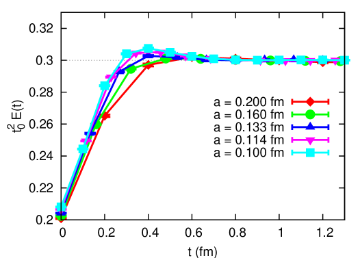
Similar boundary effects will be present in all observables. Ultimately, the physics we are interested in is infinite-volume QCD, which means the physics in the central region of Euclidean time, where measurements are independent of the boundary conditions. We will call the central region of the lattice where the physics is independent of the boundary conditions the “bulk,” in contrast to the “boundary regions” near and where open and periodic boundary conditions show significant differences. Figure 1 suggests that on our lattices a safe estimate for the width of the boundary region is fm. We also examined boundary effects in observables constructed from , such as , and found the boundary region to be no wider than that for . The width of the boundary region is presumably determined by a combination of QCD correlation lengths (inverse glueball masses, in the pure gauge theory) and the smearing radius fm of the Wilson flow [16]. The boundary region is likely narrower for observables defined without smearing.
The fact that the physics is altered in the boundary regions means that a useful comparison between periodic and open boundary conditions requires some care. The boundary regions on an open lattice are simulating physics which is not infinite-volume QCD and which has no analogue on a corresponding periodic lattice. Therefore it is not sensible to include the boundary regions in any comparison between an open ensemble and a periodic ensemble. For example, we will not compare the autocorrelations of the global topological charge on periodic and open lattices because this observable contains large contributions from the boundary regions. It turns out that autocorrelation times tend to be much shorter in the boundary regions than in the bulk, so observables with contributions from boundary regions will show artificially low autocorrelation times on open lattices compared to periodic lattices. But when the goal is to simulate infinite-volume QCD, this effect does not represent a speedup because it comes from regions of the open lattice where the physics is very different from infinite-volume QCD. The interesting question is whether autocorrelation times in the bulk are reduced by using open boundary conditions. Therefore when we discuss autocorrelations we will only make comparisons between open and periodic lattices using observables defined within the central region of Euclidean time, which we found above to have boundary-independent physics.
3.2 Measured autocorrelations of topological observables
In this section we give some measurements of autocorrelations of topological observables on our ensembles. First we briefly clarify our conventions for measures of autocorrelation. Suppose we measure some observable as a function of MD time . Then , the autocorrelation function of , is defined as
| (3.1) |
The normalized autocorrelation function and integrated autocorrelation time are defined by
| (3.2) |
where is the MD time interval at which we measure . We always report integrated autocorrelation times in molecular dynamics time units. Ref.’s [1, 5] contain useful formulas for calculating statistical errors on the estimators of these quantities.
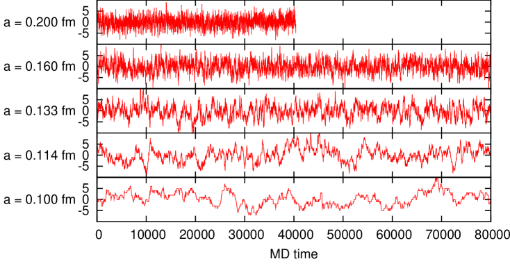
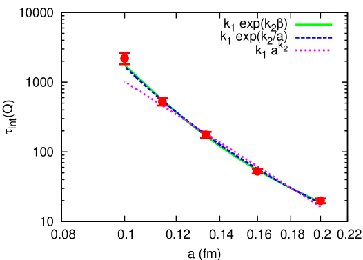
As discussed in the introduction, the global topological charge rapidly develops longer and longer autocorrelations as the lattice spacing is decreased. In Figure 2 we show portions of the MD time histories of on our periodic lattices at each simulated lattice spacing. The dramatic slowdown of as is obvious. Table 2.1 gives , the integrated autocorrelation time of the global topological charge, on each of our periodic lattices. increases by a factor of about 100 from our coarsest to our finest lattice. Figure 3 shows that we obtain a good fit to the scaling behavior of with the ansatz
| (3.3) |
This fit form is motivated by the notion that there is some action barrier to topological tunneling which should therefore be suppressed by a factor . We can also obtain a good fit using the form
| (3.4) |
A power law with , can approximately fit the data, but this fit is not as good, as Figure 3 shows.
These results for the -dependence of are quite similar to those of [1], which simulated the pure gauge theory with the Wilson gauge action, and found that both the form of Eq. (3.4) and the power law form (with exponent around ) described the data reasonably well. While we use the DBW2 gauge action and so becomes large at a coarser lattice spacing, the same fit forms apparently work reasonably well for both actions.
| (fm) | Periodic | Periodic | Open | Periodic | Open |
| 0.2000 | |||||
& 13.0(4) 13(1) 18(1) 18(1) 0.1600 53(4) 28(1) 28(2) 44(2) 41(3) 0.1326 175(18) 66(4) 62(5) 129(11) 105(9) 0.1143 525(63) 151(11) 136(11) 353(35) 270(22) 0.1000 2197(389) 465(66) 217(19) 1307(214) 464(43)
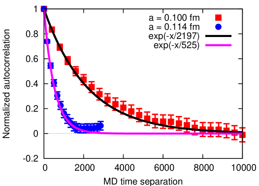
On all of our periodic lattices we find that the autocorrelation function of has the form of a single exponential to within our statistical precision. Figure 4 shows this for our two finest lattice spacings.
As discussed in Section 3.1, the global topological charge is not the best observable to use for comparisons between periodic and open lattices. We should instead look at observables defined on subvolumes that lie entirely within the bulk. For the moment we focus on two such observables: , the topological charge summed over the central time slice, and , the topological charge summed over the central half of the lattice volume.
Table 2.1 gives the integrated autocorrelation times of these observables on both periodic and open lattices at each lattice spacing. Like , these integrated autocorrelation times rise very rapidly as the lattice spacing is reduced. However, the -dependence of these autocorrelation times is not captured by a simple function like Eq. (3.3) or (3.4). We determine the scaling behavior of these autocorrelation times in Section 4 below. Note that the half-volume charge always has a significantly longer autocorrelation time than the time-slice charge .
The results of Table 2.1 show that open boundary conditions do indeed lead to reduced (but still quite long) autocorrelation times at fine enough lattice spacings. At the very finest lattice spacing, fm, open boundary conditions produce a more than a factor of 2 reduction in the integrated autocorrelation times. At fm and 0.133 fm, the next two finest lattice spacings, open boundary conditions show slightly shorter autocorrelations than periodic boundary conditions, with the improvement clearer for the half-volume charge . At the two coarsest lattice spacings the integrated autocorrelation times are independent of the boundary conditions to within the limits of our measurements.
The reason for the difference between periodic and open boundary conditions at fine lattice spacings is exactly that envisaged in [5]. At fine lattice spacings on periodic lattices, the autocorrelation functions of topological observables like the time-slice charge and the half-volume charge develop long tails proportional to the autocorrelation function of the global charge. As the autocorrelation time of the global charge becomes very long, so do these tails. Autocorrelation functions on open lattices do not develop such long tails, because the global charge does not slow down as drastically. On open lattices the topological charge can flow in and out through the boundaries and so the global charge can change without having to wait for rare tunneling events. Figure 5 demonstrates this, comparing the autocorrelation function of the half-volume charge between open and periodic boundary conditions at the coarsest and finest lattice spacings.
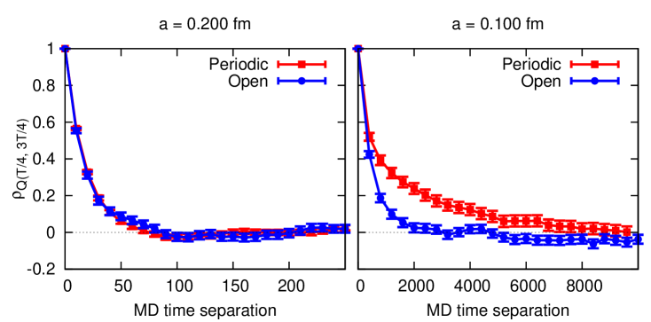
In the rest of this paper we will develop a model for topological autocorrelations which will precisely reproduce the measured autocorrelation functions of topological observables, such as those plotted in Figure 5. Among other things this model lets us predict the lattice spacing at which integrated autocorrelation times on periodic lattices start to become much longer than those on open lattices. Thus the model will tell us when open boundary conditions start to become useful for reducing autocorrelations.
4 Diffusion of topological charge
The mechanism by which the global topological charge changes during an HMC evolution is moderately well-understood. As discussed in the introduction, the global charge on a periodic lattice can only change via lattice artifacts: “tears” or “dislocations” in the gauge field where the field is not smooth and continuum-like. These dislocations are likely to be small structures, with size of order the lattice scale, in order to minimize their action. When the global topological charge changes by means of one of these dislocations we speak of the lattice gauge field tunneling between adjacent topological sectors. The rate of tunneling can be quantified by, for example, the integrated autocorrelation time of the global topological charge.
Less well-understood is how the topological charge moves around the lattice in the absence of these tunneling events. In particular, when considering open boundary conditions it would be very useful to know how fast this motion is, because open boundary conditions are supposed to reduce autocorrelations by allowing topological charge to be created or destroyed at the open boundaries and then move into the bulk of the lattice. The effectiveness of open boundary conditions will therefore be directly related to the speed at which topological charge moves through the lattice in the absence of tunneling. (This question is also interesting for simulations which deliberately run in a fixed topological sector; then the rate at which charge moves around will determine how long it takes the lattice to decorrelate within a given topological sector.)
One of the strengths of the mathematical model we will now develop is that it provides a clean and quantitative definition of the vague notion of “how fast topological charge moves around the lattice.” This will enable us to develop a theoretical understanding of the circumstances in which open boundary conditions will reduce autocorrelations.
4.1 The diffusion model
In this section we give a mathematical model that reproduces the autocorrelation function of , the topological charge summed over a single time slice. With this model we will be able to determine the scaling behavior of the autocorrelation times of Section 3.2 and we will show how to determine the lattice spacing at which the autocorrelation times measured on open and periodic lattices start to differ.
Denote by the topological charge summed over the time slice with Euclidean time coordinate on the configuration at MD time . We will focus on the correlation function222Henceforth “” will always be a Euclidean time and should not be confused with the Wilson flow reference time.
| (4.1) |
This correlation function tells us about the movement of topological charge through the lattice during the HMC evolution. Roughly speaking, will be large when a lump of topological charge present on time slice at some MD time is likely to move to time slice by MD time . As a special case, is the autocorrelation function of .
We can measure the correlation function straightforwardly with our high statistics. We find empirically that it obeys a simple diffusion-decay equation:333This generalization of the diffusion equation to a position-dependent diffusion coefficient is just one of many possibilities. This form is the first that we tried and we found it to work well. Later we tried altering the diffusion term to . This form also works well but led to slightly larger values of the defined in Eq. (4.6)
| (4.2) |
Here the derivatives with respect to Euclidean time should be understood as finite differences and is a function defined at Euclidean times midway between the lattice time slices. We will call Eq. (4.2) the “diffusion model.” The free parameters of the model are the function and the quantity .
is a -dependent diffusion coefficient with units of . It quantifies how fast topological charge diffuses in the Euclidean time direction and answers the question raised above of how fast topological charge moves around the lattice in the absence of tunneling events. By time-translation invariance, is a constant function on periodic lattices or in the bulk region of open lattices, but it can have nontrivial -dependence near open boundaries. In fact we will find in Section 4.2 that is somewhat enhanced in the immediate vicinity of an open boundary. However, we will often treat as a constant, , unless we are interested in this boundary effect.
, which we call the “tunneling timescale,” has units of MD time and quantifies the rate of tunneling between topological sectors. In fact, on a periodic lattice it is exactly the integrated autocorrelation time of the global topological charge. This can be seen as follows. Summing over and gives the autocorrelation function of the global topological charge:
| (4.3) |
where here denotes the global topological charge at MD time . Then if we sum Eq. (4.2) over and , the diffusion term drops out because it is a total derivative, leaving
| (4.4) |
This implies that the autocorrelation function of the global charge is a simple exponential, as found in Section 3.2, and that the area under the normalized autocorrelation function is , as claimed. Thus on periodic lattices we have .
In principle, could be a function of Euclidean time near an open boundary. However, we are unable to resolve any such -dependence in our data, and so we always take to be a constant throughout the lattice.
The boundary conditions satisfied by the correlation function depend on the boundary conditions for the lattice gauge field. On periodic lattices is periodic in and in . On open lattices goes to zero at the Euclidean time boundaries in the continuum limit:
| (4.5) |
These boundary conditions let the correlations measured by “leak out” through the open boundaries, just as the topological charge itself can leak out. They arise from the fact that open boundary conditions correspond to setting the color-electric field to zero at the boundaries [5]. Therefore the topological charge density, which is proportional to , also vanishes at the boundaries, as do correlation functions of the charge density such as .
The diffusion model provides a concrete way of thinking about how the topological charge density changes during an HMC evolution. There are two processes: a diffusion process that proceeds at a rate given by and a tunneling process that proceeds at a rate given by . As we will now demonstrate, this simple model suffices to completely explain our measurements of the autocorrelations of topological observables. The integrated autocorrelation time is of course a well-known quantity but as far as we know the diffusion coefficient has not been identified before.
4.2 Diffusion model fits to simulation data
In this section we discuss our method for estimating the free parameters of Eq. (4.2) from our data and demonstrate the close agreement between the model and our simulation data.
Eq. (4.2) predicts for MD time separations given the “initial condition” , which gives the correlations between the at zero MD time separation. The free parameters in the differential equation are the diffusion coefficient and the tunneling timescale . must be a constant function on periodic lattices, but on open lattices we allow it to be a general function of , except that we impose time-reversal symmetry (i.e., symmetry under ). So on periodic lattices, the model has two free parameters, and , while on open lattices the model has free parameters, and the values of for .
For a given choice of the parameters and , we define a measure of the goodness of fit as follows. We measure the function from our data, then numerically integrate Eq. (4.2) to obtain the prediction for the correlation function at , which we will denote by . We then measure the function from our data, obtaining an estimate with statistical error . These measurements are made for a discrete set of MD time separations , . Finally we define the goodness of fit
| (4.6) |
We find the best estimates of and by varying them to minimize this . Finally we estimate statistical errors on and by the jackknife method. We use a blocked jackknife with blocks much longer than the longest measured autocorrelation time.
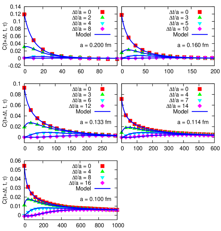
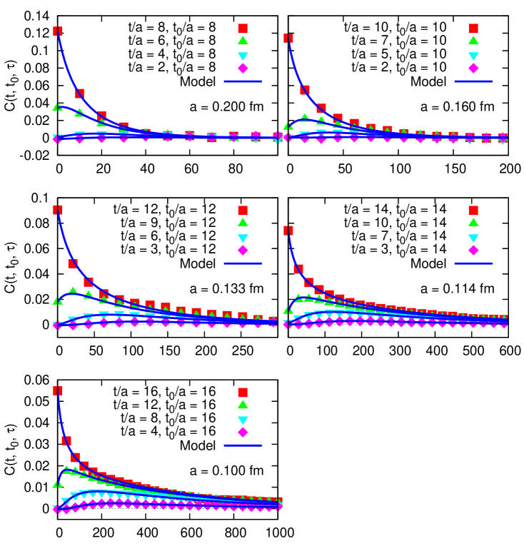
The resulting fits are shown in Figures 6 and 7 where for each ensemble we plot for several choices of and alongside the model fit. In every case our simple model produces remarkably good agreement with the measured correlation functions. We stress that and are determined only once per ensemble: the in Eq. (4.6) sums over all values of and . After minimizing , the resulting estimates for and are used to predict the for any and any .
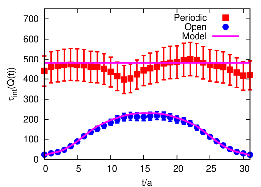
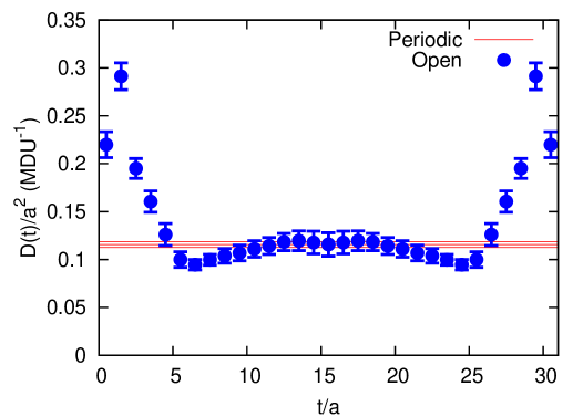
We can integrate the diffusion model predictions for autocorrelation functions to get predictions for integrated autocorrelation times. Figure 8 compares measurements of , the integrated autocorrelation time of , to model predictions on our finest pair of ensembles. The predictions are computed using the estimates of and from the above fitting procedure. There is close agreement, and the diffusion model correctly reproduces the nontrivial -dependence of in the presence of open boundary conditions.
The best estimates for and (the diffusion coefficient at the center of the lattice) are summarized in Table 2.1. At a given lattice spacing, the measured values of these quantities on the periodic and open lattices are consistent with each other. This is expected: the boundary conditions should not affect the rate of tunneling or diffusion in the bulk. Furthermore, the measured values of in Table 2.1 are consistent with the measured values of the integrated autocorrelation time on periodic lattices in Table 2.1, as expected since Eq. (4.4) predicts . The estimates from open lattices tend to have larger error bars: this is because the model has more free parameters on open lattices since is allowed to depend on .
& 20(2) 0.090(12) 0.099(30) 0.1600 56(3) 51(3) 0.1018(73) 0.113(18) 0.1326 185(20) 162(19) 0.1085(97) 0.088(15) 0.1143 561(59) 737(143) 0.1080(56) 0.120(14) 0.1000 2350(389) 1973(621) 0.1155(29) 0.116(12)
While is identical in the bulk between periodic and open lattices, when is close to an open boundary we observe that is enhanced relative to its bulk value. As an example, Figure 9 shows the fit results for the function at our finest lattice spacing, comparing the open result to the (time-translation invariant) periodic result.
is a property of the HMC algorithm and not a physical observable. However, we expect that the width of the boundary region in which is enhanced is controlled, as for physical observables, by a combination of the Wilson flow smearing radius and QCD correlation lengths.
4.3 Scaling of the diffusion coefficient
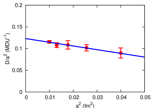
In Section 3.2 we gave some fits to the -dependence of , which is identical to the diffusion model parameter . It is very interesting to ask how the diffusion coefficient , the other parameter of the diffusion model, depends on the lattice spacing. The answer is that over the range of lattice spacings we simulated scales like up to small corrections. Figure 10 plots the fit results for as a function of on periodic lattices, finding good agreement with a fit of the form
| (4.7) |
As we will discuss below in Section 4.7, the parameters and depend on the parameters of the HMC algorithm, in particular the trajectory length. In our simulations, we have chosen to scale the trajectory length like . It may be that a different choice for the scaling of the trajectory length would lead to different scaling behaviors for and . In the rest of this paper we will assume that scales like , but it should be kept in mind that this could be modified to some extent by difference choices for the scaling of the trajectory length.
The diffusion coefficient and the lattice Euclidean time extent together define a characteristic MD time we will call the “diffusion timescale,”
| (4.8) |
With the factor of 8 included, this is roughly the MD time it takes a lump of topological charge to diffuse across a distance . It should be thought of as the speed at which the center of the lattice can communicate with the boundaries. From the scaling of , the characteristic MD time interval scales like at fixed Euclidean time extent .
4.4 The tunneling- and diffusion-dominated regimes
The diffusion model thus identifies a tunneling timescale and a diffusion timescale . There are two limiting cases where one of these timescales is much shorter than the other. In the “tunneling-dominated” regime characterized by , diffusion is much slower than tunneling, while in the “diffusion-dominated” regime where diffusion is much faster than tunneling.
The tunneling-dominated regime corresponds to large (because then tunneling is fast) or large (because then it takes a long time to diffuse across the lattice). Conversely the diffusion-dominated regime corresponds to small or small . For a fixed physical value of , coarse enough lattices will be tunneling-dominated while fine enough lattices will be diffusion-dominated. Similarly, for a fixed value of , short enough lattices will be diffusion-dominated while long enough lattices will be tunneling-dominated.
The transition region between these regimes is the region of parameter space where . Given the measurements of and shown in Figure 11, this happens in our set of ensembles at fm. It should be kept in mind that the transition between the tunneling- and diffusion-dominated regimes will happen at a different lattice spacing depending on the action, Euclidean time extent, and the HMC algorithm parameters. For example, if we used an action that was better at topological tunneling, such as the Wilson gauge action, this transition would occur at a finer lattice spacing.

Tunneling happens at equal rates on periodic and open lattices. Therefore in the tunneling-dominated regime there will be little difference between the autocorrelation times on periodic and open lattices. Because is so short, autocorrelations are destroyed by tunneling much faster than the timescale on which the boundaries can affect the bulk. In the diffusion-dominated regime, however, we expect significant differences between autocorrelation times on open and periodic lattices. On open lattices, in the diffusion-dominated regime, the topological charge in the bulk can change even in the absence of tunneling by exchanging topological charge with the boundaries, where topological charge can be created and destroyed freely.
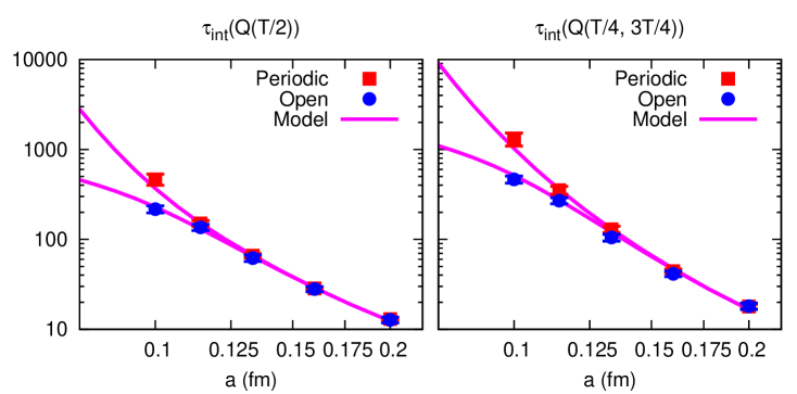
Figure 12 shows that the integrated autocorrelation times of the time slice charge and the half-volume charge both follow this pattern. At coarse lattice spacings, periodic and open boundary conditions produce identical autocorrelation times. At fine lattice spacings, open boundary conditions produce much shorter autocorrelation times. The transition region between these two regimes indeed occurs at fm.
Also plotted in Figure 12 are the integrated autocorrelation times for these observables calculated with the diffusion model, using as inputs the measured scaling behavior of and (we have neglected the boundary region enhancement of on open lattices, which has only a minor effect on these integrated autocorrelation times). The model curves correctly reproduce the observed behavior and show that if we ran simulations at even finer lattice spacings the difference between periodic and open boundary conditions would become very large.
How exactly do autocorrelation times scale with ? How much do open boundary conditions improve the scaling the diffusion-dominated regime? In principle to answer these questions all we have to do is numerically integrate Eq. (4.2), making use of our knowledge of the simple -dependence of and . That is what we have done in Figure 12. However, we can do better: in the tunneling- or diffusion-dominated limits we can obtain analytic results for some integrated autocorrelation times in the diffusion model. We work these out in the next section.
4.5 Analytic scaling laws in the tunneling- and diffusion-dominated regimes
In this section we use Eq. (4.2) to compute the integrated autocorrelation time of , the topological charge on the time slice at Euclidean time , in the tunneling- and diffusion-dominated regimes on periodic and open lattices. We will obtain analytic results telling us how this integrated autocorrelation time scales with in each of these limits. While we will carry out the computations for the specific observable , some of the results will generalize to all topological observables.
In these calculations we make a few simplifications to make the problem more analytically tractable. First, we will treat Euclidean time as continuous, so that the ’s in Eq. (4.2) will be actual derivatives instead of finite differences. This is a good approximation because is always fairly smooth as a consequence of the Wilson flow smearing that goes into measuring . Second, we will ignore the fact that in real simulations measurements are only conducted at discrete MD times separated by an interval ; we will simply compute the integrated autocorrelation time as an integral:
| (4.9) |
whereas in an actual simulation would have to be computed as a discrete sum. Finally, we will ignore the -dependence of near the open boundaries, which will not change the qualitative conclusions as long as is significantly larger than the boundary region in which is not constant.
In order to make predictions we need as input the equal-MD-time correlation function . In our simulations, we find that is very close to Gaussian:
| (4.10) |
where is a physical length scale which we find to be about 0.22 fm. The scaling predictions in this section use this Gaussian form for . However the exact shape of is not important for the qualitative conclusions we will draw about scaling.
With these simplifications the problem amounts to solving the simple linear differential equation Eq. (4.2) with initial conditions given by Eq. (4.10) and then performing the integral in Eq. (4.9). We relegate the details to an appendix and just give the results here.
4.5.1 The tunneling-dominated regime
In the tunneling dominated regime, autocorrelation times are independent of the boundary conditions for observables located far enough from the boundaries. Here “far enough” means a distance greater than about . If satisfies this condition, we find
| (4.11) |
where the approximation is good up to corrections down by powers of . These corrections become small at fine enough lattice spacings, well before the lattice spacing becomes fine enough that we transition from the tunneling-dominated to the diffusion-dominated regime. Eq. (4.11) says that in the tunneling-dominated regime this integrated autocorrelation time scales essentially like . This scaling is not quite as bad as that of itself but it is still quite bad. We will now see that the scaling in the diffusion-dominated regime is worse than this on periodic lattices, but better than this on open lattices.
4.5.2 The diffusion-dominated regime on periodic lattices
On a periodic lattice, the large- behavior of the normalized autocorrelation function of is:
| (4.12) |
In the diffusion-dominated limit, is very large and becomes dominated by the area under this tail, so that
| (4.13) |
So on periodic lattices in the diffusion-dominated regime, scales in the same (very bad) way as , the integrated autocorrelation time of the global topological charge.
This result generalizes beyond the time-slice charge: in the diffusion-dominated limit on a periodic lattice all topological autocorrelation times scale like , and thus increase very rapidly as . The reason is that all topological autocorrelation functions develop long tails of the form with , and for large enough the area under this tail dominates the integrated autocorrelation time.
4.5.3 The diffusion-dominated regime on open lattices
On an open lattice in the diffusion-dominated limit, we find
| (4.14) |
where is a near-unity coefficient. This formula gives the form of the -dependence of on open lattices, although it should be kept in mind that the exact form of the -dependence will be modified by the time-dependence of the diffusion coefficient near the boundaries, which we have neglected in this calculation.
Eq. (4.14) shows that in the diffusion-dominated regime scales in the same way as . Above we found that scales like , so in this regime the integrated autocorrelation time of scales like . In fact this scaling behavior generalizes to all topological autocorrelation times. This is because in the diffusion-dominated limit on open lattices the term in Eq. (4.2) proportional to can be dropped. Then any quantity with units of MD time that we can construct from the parameters of the diffusion model is proportional to . Thus in the diffusion-dominated limit on open lattices, all topological autocorrelation times scale like .
Finally, we see that at fixed this integrated autocorrelation time is proportional to . So while the scaling is an improvement over the scaling seen with periodic boundary conditions, if the lattice has a large Euclidean time extent the coefficient in front of the will be large.
4.6 More general topological observables
The mathematical model we have given describes the MD-time correlation functions of the time-slice topological charges . We can combine these to find the autocorrelation function of , the charge summed over a finite Euclidean time extent by expressing the subvolume charge as a sum of time slice charges:
| (4.15) |
where here is the value of the subvolume charge at the MD time . The diffusion model gives all the correlation functions on the right-hand side, so we can use it to compute the left-hand side also. For example, in Figure 13 we plot the normalized autocorrelation functions of several subvolume charges on the periodic fm ensemble and demonstrate that they are in close agreement with the model predictions calculated using Eq. (4.15).
We can also use the model to compute the autocorrelations of squared charges like and . As noted in [5], if is any observable defined by a sum over a region of the lattice much larger than the longest physical QCD correlation length, then there is a simple relationship
| (4.16) |
between the normalized autocorrelation function of and the normalized autocorrelation function of . Thus for instance we can predict the normalized autocorrelation function of just by squaring the prediction for the normalized autocorrelation function of .

4.7 Dependence of diffusion model parameters on HMC algorithm parameters
Autocorrelation times are properties of the HMC algorithm and not properties of the simulated theory alone. Therefore the tunneling and diffusion timescales that we have defined may depend not just on the lattice spacing and the Euclidean time extent but also on the parameters of the simulation algorithm. Here the only parameter we will consider is the trajectory length.
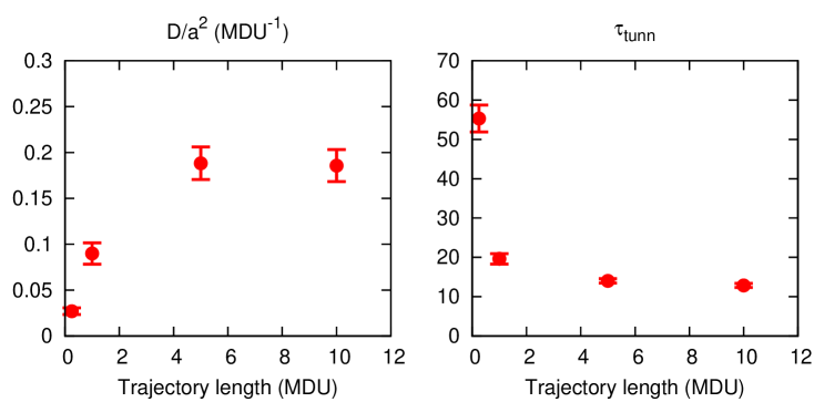
We ran several additional simulations with different HMC trajectory lengths at our coarsest lattice spacing in order to measure the influence of the trajectory length on the diffusion coefficient and the tunneling timescale . The measurement interval MDU was held constant as the trajectory length was varied, and the MD integrator step size was adjusted to keep acceptance high. As shown in Figure 14, we find that longer trajectories lead to larger and smaller . This is consistent with previous experience which suggests that increasing the trajectory length can decrease autocorrelation times [17, 1].
5 Conclusions
We have shown that the autocorrelation functions of topological observables are predicted very accurately by a surprisingly simply mathematical model that incorporates only two processes: diffusion of topological charge and tunneling between topological sectors. The rates of these processes are given by the diffusion coefficient and the tunneling timescale (which on a periodic lattice is just the integrated autocorrelation time of the global topological charge). We find that scales like while scales like with uncomfortably large.
The relative rates of the tunneling process and the diffusion process determine whether open boundary conditions are useful for reducing autocorrelation times. The characteristic timescale of the diffusion process is . Open boundary conditions show drastically improved scaling of autocorrelation times in the diffusion-dominated regime, when
| (5.1) |
In this regime, topological autocorrelation times scale like on open lattices, while on periodic lattices they are proportional to . It is when Eq. (5.1) is satisfied that open boundary conditions are useful for reducing autocorrelation times.
In the opposite limit of the simulation is tunneling-dominated. In this regime autocorrelation times in the bulk are independent of the boundary conditions and open boundary conditions will not reduce autocorrelation times.
As an example of applying this criterion, we can consider the Wilson gauge action simulations of [6], mentioned in the introduction, in which we attempted to compare open and periodic boundary conditions with the Wilson gauge action at , fm, . The statistics of those simulations were quite low given the long autocorrelations, but we can estimate the order of magnitude of the tunneling timescale from the high-statistics simulations of [1]. There a simulation with the same gauge action (but a slightly different simulation algorithm) at the nearby value of found the integrated autocorrelation time of to be several thousand MDU; this gives the right order of magnitude for , which is the integrated autocorrelation time of . Meanwhile if the diffusion constant for the Wilson gauge action is similar to the value measured here with the DBW2 action, then the diffusion timescale is MDU. The situation is therefore likely similar to the DBW2 lattices at fm in this paper: is smaller than by a factor of a few, so open boundary conditions should decrease autocorrelation times by a factor of a few. However both timescales are quite long, and with the limited statistics we collected in [6] we were not able to measure the long autocorrelations accurately enough to detect this difference.
Eq. (5.1) will be satisfied eventually for small enough , so open boundary conditions will always be useful if the lattice spacing is fine enough. How small needs to be depends on the lattice action (which controls the tunneling timescale) and the Euclidean time extent. The faster the tunneling timescale and the longer the lattice, the finer the lattice spacing needs to be before open boundary conditions will be useful. Long lattices have an additional drawback: in the diffusion-dominated regime on open lattices some integrated autocorrelation times are proportional to .
6 Acknowledgements
We thank Martin Lüscher and Stefan Schaefer as well as our fellow members of the RBC collaboration for useful conversations. We thank RIKEN-BNL Research Center and Brookhaven National Lab for the use of the Blue Gene/Q computers. This work was supported by US DOE grant #DE-FG02-92ER40699.
Appendix A Appendix: Analytic calculation of
Here we supply some of the details in the calculations of in Section 4.5.
For convenience we will scale so that ; then the normalized autocorrelation function of is .
A.1 The tunneling-dominated regime
In the tunneling-dominated regime, as long as is not too close to an open boundary we can pretend that we are working with a lattice of infinite Euclidean time extent, because the correlations measured by are destroyed by tunneling before they can diffuse to the boundaries of the lattice. Solving Eq. (4.2) on an infinite domain with initial conditions given by Eq. (4.10) we obtain
| (A.1) |
The normalized autocorrelation function of is then
| (A.2) |
and the integrated autocorrelation time is
| (A.3) |
where .
A.2 The diffusion-dominated regime on periodic lattices
At finite , Eq. (4.2) can be solved by solving the eigenvalue equation
| (A.4) |
where the satisfy periodic boundary conditions, and then expanding in the eigenmodes as
| (A.5) |
The integrated autocorrelation time of is then
| (A.6) |
Without loss of generality we will take . The eigenfunctions and eigenvalues are
| (A.7) |
where we have ignored the odd eigenfunctions of Eq. (A.4) because they are orthogonal to the initial state . In the diffusion-dominated limit, becomes large and so becomes much smaller than all the other eigenvalues. In this limit, the normalized autocorrelation function develops a long tail at large :
| (A.8) |
In the diffusion-dominated limit, becomes dominated by the area under this tail, so that
| (A.9) |
A.3 The diffusion-dominated regime on open lattices
On open lattices we again must solve the eigenvalue problem Eq. (A.4) but this time the boundary conditions are . The eigenfunctions and eigenvalues are
| (A.10) |
This time there is no near-zero eigenvalue when becomes large, so the sum in Eq. (A.6) is not dominated by a single mode. Therefore in the diffusion-dominated limit we can drop the term in Eq. (A.10). For , a good approximation is
| (A.11) |
For , goes rapidly to zero. Then using Eq. (A.6) we can write a good approximation to :
| (A.12) |
We can extend this finite sum to an infinite sum at the cost of an error. Then using the fact that, for ,
| (A.13) |
we get
| (A.14) |
where is some coefficient of order that accounts for the error introduced by going from a finite sum to an infinite one.
References
- [1] S. Schaefer et al. [ALPHA Collaboration], “Critical slowing down and error analysis in lattice QCD simulations,” Nucl. Phys. B 845, 93 (2011) [arXiv:1009.5228 [hep-lat]].
- [2] L. Del Debbio, H. Panagopoulos and E. Vicari, “ dependence of SU(N) gauge theories,” JHEP 0208, 044 (2002) [hep-th/0204125].
- [3] M. Lüscher, “Topology, the Wilson flow and the HMC algorithm,” PoS LATTICE 2010, 015 (2010) [arXiv:1009.5877 [hep-lat]].
- [4] M. Lüscher, “Step scaling and the Yang-Mills gradient flow,” arXiv:1404.5930 [hep-lat].
- [5] M. Lüscher and S. Schaefer, “Lattice QCD without topology barriers,” JHEP 1107, 036 (2011) [arXiv:1105.4749 [hep-lat]].
- [6] G. McGlynn and R. D. Mawhinney, “Scaling, topological tunneling and actions for weak coupling DWF calculations,” PoS Lattice 2013, 027 (2013) [arXiv:1311.3695 [hep-lat]].
- [7] A. Chowdhury, A. Harindranath, J. Maiti and P. Majumdar, “Topological susceptibility in lattice Yang-Mills theory with open boundary condition,” JHEP 1402, 045 (2014) [arXiv:1311.6599 [hep-lat]].
- [8] M. Bruno and R. Sommer, “On the -dependence of gluonic observables,” PoS LATTICE 2013, 321 (2013) [arXiv:1311.5585 [hep-lat]].
- [9] T. Takaishi, “Heavy quark potential and effective actions on blocked configurations,” Phys. Rev. D 54, 1050 (1996).
- [10] Y. Aoki, T. Blum, N. Christ, C. Cristian, C. Dawson, T. Izubuchi, G. Liu and R. Mawhinney et al., “Domain wall fermions with improved gauge actions,” Phys. Rev. D 69, 074504 (2004) [hep-lat/0211023].
- [11] M. A. Clark, B. Joo, A. D. Kennedy and P. J. Silva, “Improving dynamical lattice QCD simulations through integrator tuning using Poisson brackets and a force-gradient integrator,” Phys. Rev. D 84, 071502 (2011) [arXiv:1108.1828 [hep-lat]].
- [12] H. Yin and R. D. Mawhinney, “Improving DWF Simulations: the Force Gradient Integrator and the Möbius Accelerated DWF Solver,” PoS LATTICE 2011, 051 (2011) [arXiv:1111.5059 [hep-lat]].
- [13] S. A. Gottlieb, W. Liu, D. Toussaint, R. L. Renken and R. L. Sugar, “Hybrid Molecular Dynamics Algorithms for the Numerical Simulation of Quantum Chromodynamics,” Phys. Rev. D 35, 2531 (1987).
- [14] S. Necco, “Universality and scaling behavior of RG gauge actions,” Nucl. Phys. B 683, 137 (2004) [hep-lat/0309017].
- [15] P. de Forcrand, M. Garcia Perez and I. -O. Stamatescu, “Topology of the SU(2) vacuum: A Lattice study using improved cooling,” Nucl. Phys. B 499, 409 (1997) [hep-lat/9701012].
- [16] M. Lüscher, “Properties and uses of the Wilson flow in lattice QCD,” JHEP 1008, 071 (2010) [Erratum: JHEP 1403, 092 (2014)] [arXiv:1006.4518 [hep-lat]].
- [17] H. B. Meyer, H. Simma, R. Sommer, M. Della Morte, O. Witzel and U. Wolff, “Exploring the HMC trajectory-length dependence of autocorrelation times in lattice QCD,” Comput. Phys. Commun. 176, 91 (2007) [hep-lat/0606004].