Arc-Search Infeasible Interior-Point Algorithm for Linear Programming

Abstract

Mehrotra’s algorithm has been the most successful infeasible interior-point algorithm for linear programming since 1990. Most popular interior-point software packages for linear programming are based on Mehrotra’s algorithm. This paper proposes an alternative algorithm, arc-search infeasible interior-point algorithm. We will demonstrate, by testing Netlib problems and comparing the test results obtained by arc-search infeasible interior-point algorithm and Mehrotra’s algorithm, that the proposed arc-search infeasible interior-point algorithm is a more efficient algorithm than Mehrotra’s algorithm.

Keywords: Arc-search, infeasible interior-point algorithm, linear programming.

1 Introduction

Interior-point method is now regarded as a mature technique of linear programming [1, page 2], following many important developments in 1980-1990, such as, a proposal of path-following method [2], the establishment of polynomial bounds for path-following algorithms [3, 4], the development of Mehrotra’s predictor-corrector (MPC) algorithm [5] and independent implementation and verification [6, 7], and the proof of the polynomiality of infeasible interior-point algorithm [8, 9]. Although many more algorithms have been proposed since then (see, for example, [10, 11, 12, 13, 14]), there is no significant improvement in the best polynomial bound for interior-point algorithms, and there is no report of a better algorithm than MPC for general linear programming problems. In fact, the most popular interior-point method software packages implemented MPC, for example, LOQO [16], PCx [17] and LIPSOL [18].

However, there were some interesting results obtained in recent years. For example, higher-order algorithms that used second or higher-order derivatives were demonstrated to improve the computational efficiency [5, 7]. Higher-order algorithms, however, had either a poorer polynomial bound than first-order algorithms [19] or did not even have a polynomial bound [5, 20]. This dilemma was partially solved in [21] which proved that higher-order algorithms can achieve the best polynomial bound. An arc-search interior-point algorithm for linear programming was devised in [21]. The algorithm utilized the first and second-order derivatives to construct an ellipse to approximate the central path. Intuitively, searching along this ellipse should generate a larger step size than searching along any straight line. Indeed, it was shown in [21] that the arc-search algorithm has the best polynomial bound and it may be very efficient in practical computation. This result was extended to prove a similar result for convex quadratic programming and the numerical test result was very promising [22].

The algorithms proposed in [21, 22] assume that the starting point is feasible and the central path does exist. Available Netlib test problems are limited because most Netlib problems may not even have an interior-point as noted in [23]. To better demonstrate the claims in the previous papers, we propose an infeasible arc-search interior-point algorithm in this paper, which allows us to test a lot more Netlib problems. The proposed algorithm keeps a nice feature developed in [21, 22], i.e., it searches optimizer along an arc (part of an ellipse). It also adopts some strategies used in MPC, such as using different step sizes for the vector of primal variables and the vector of slack variables. We will show that the proposed arc-search infeasible interior-point algorithm is very competitive in computation by testing all Netlib problems in standard form and comparing the results to those obtained by MPC. To have a fair comparison, both algorithms are implemented in MATLAB; for all test problems, the two Matlab codes use the same pre-processor, start from the same initial point, use the same parameters, and terminate with the same stopping criterion. Since the main cost in computation for both algorithms is to solve linear systems of equations which are exactly the same for both algorithms, and the arc-search infeasible interior-point algorithm uses less iterations in most tested problems than MPC, we believe that the proposed algorithm is more attractive than the MPC algorithm.

The remaining of the paper is organized as follows. Section 2 briefly describes the problem. Section 3 presents the proposed algorithm and some simple but important properties. Section 4 discusses implementation details for both algorithms. Section 5 provides numerical results and compares the results obtained by both arc-search method and Mehrotra’s method. Conclusions are summarized in Section 6.

2 Problem Descriptions

Consider the Linear Programming in the standard form:

$$\min\hskip 3.61371ptc^{{\rm T}}x,\hskip 10.84006pt\mbox{\rm subject to}\hskip 7.22743ptAx=b,\hskip 7.22743ptx\geq 0,$$ (1)

where $A\in{\bf R}^{m\times n}$, $b\in{\bf R}^{m}$, $c\in{\bf R}^{n}$ are given, and $x\in{\bf R}^{n}$ is the vector to be optimized. Associated with the linear programming is the dual programming that is also presented in the standard form:

$$\max\hskip 3.61371ptb^{{\rm T}}\lambda,\hskip 10.84006pt\mbox{\rm subject to}\hskip 7.22743ptA^{{\rm T}}\lambda+s=c,\hskip 7.22743pts\geq 0,$$ (2)

where dual variable vector $\lambda\in{\bf R}^{m}$, and dual slack vector $s\in{\bf R}^{n}$.

Throughout the paper, we will denote the residuals of the equality constraints (the deviation from the feasibility) by

$$r_{b}=Ax-b,\hskip 7.22743ptr_{c}=A^{{\rm T}}\lambda+s-c,$$ (3)

the duality measure by

$$\mu=\frac{x^{{\rm T}}s}{n},$$ (4)

the $i$th component of $x$ by $x_{i}$, the Euclidean norm of $x$ by $\|x\|$, the identity matrix of any dimension by $I$, the vector of all ones with appropriate dimension by $e$, the Hadamard (element-wise) product of two vectors $x$ and $s$ by $x\circ s$. To make the notation simple for block column vectors, we will denote, for example, a point in the primal-dual problem $[x^{{\rm T}},\lambda^{{\rm T}},s^{{\rm T}}]^{{\rm T}}$ by $(x,\lambda,s)$. We will denote a vector initial point of any algorithm by $(x^{0},\lambda^{0},s^{0})$, the corresponding scalar duality measure by $\mu_{0}$, the point after the $k$th iteration by $(x^{k},\lambda^{k},s^{k})$, the corresponding duality measure by $\mu_{k}$, the optimizer by $(x^{*},\lambda^{*},s^{*})$, the corresponding duality measure by $\mu_{*}$. For $x\in{\bf R}^{n}$, we will denote a related diagonal matrix by $X\in{\bf R}^{n\times n}$ whose diagonal elements are components of the vector $x$.

The central path ${\cal C}(t)$ of the primal-dual linear programming problem is parameterized by a scalar $t\geq 0$ as follows. For each interior point $(x,\lambda,s)\in{\cal C}(t)$ on the central path, there is a $t\geq 0$ such that

$$Ax=b$$ (5a)

$$A^{{\rm T}}\lambda+s=c$$ (5b)

$$(x,s)\geq 0$$ (5c)

$$x_{i}s_{i}=t,\hskip 7.22743pti=1,\ldots,n.$$ (5d)

Therefore, the central path is an arc in ${\bf R}^{2n+m}$ parameterized as a function of $t$ and is denoted as

$${\cal C}(t)=\{(x(t),\lambda(t),s(t)):t\geq 0\}.$$ (6)

As $t\rightarrow 0$, the central path $(x(t),\lambda(t),s(t))$ represented by (5) approaches to a solution of LP represented by (1) because (5) reduces to the KKT condition as $t\rightarrow 0$.

Because of high cost of finding an initial feasible point and the central path described in (5), we consider a modified problem which allows infeasible initial point.

$$Ax-b=r_{b}$$ (7a)

$$A^{{\rm T}}\lambda+s-c=r_{c}$$ (7b)

$$(x,s)\geq 0$$ (7c)

$$x_{i}s_{i}=t,\hskip 7.22743pti=1,\ldots,n.$$ (7d)

We search the optimizer along an infeasible central path neighborhood. The infeasible central path neighborhood ${\cal F}(\gamma)$ considered in this paper is defined as a collection of points that satisfy the following conditions,

$${\cal F}(\gamma(t))=\{(x,\lambda,s):\|(r_{b}(t),r_{c}(t))\|\leq\gamma(t)\|(r_{b}^{0},r_{c}^{0})\|,\hskip 0.72229pt(x,s)>0\},$$ (8)

where $r_{b}(1)=r_{b}^{0}$, $r_{c}(1)=r_{c}^{0}$, $\gamma(t)\in[0,1]$ is a monotonic function of $t$ such that $\gamma(1)=1$ and $\gamma(t)\rightarrow 0$ as $t\rightarrow 0$. It is worthwhile to note that this central path neighborhood is the widest in any neighborhood considered in existing literatures.

3 Arc-Search Algorithm for Linear Programming

Starting from any point $(x^{0},\lambda^{0},s^{0})$ in a central path neighborhood that satisfies $(x^{0},s^{0})>0$, for $k\geq 0$, we consider a special arc parameterized by $t$ and defined by the current iterate as follows:

$$Ax(t)-b=tr_{b}^{k},$$ (9a)

$$A^{{\rm T}}\lambda(t)+s(t)-c=tr_{c}^{k},$$ (9b)

$$(x(t),s(t))>0,$$ (9c)

$$x(t)\circ s(t)=tx^{k}\circ s^{k}.$$ (9d)

Clearly, each iteration starts at $t=1$; and $(x(1),\lambda(1),s(1))=(x^{k},\lambda^{k},s^{k})$. We want the iterate stays inside ${\cal F}(\gamma)$ as $t$ decreases. We denote the infeasible central path defined by (9) as

$${\cal H}(t)=\{(x(t),\lambda(t),s(t)):t\geq\tau\geq 0\}.$$ (10)

If this arc is inside ${\cal F}(\gamma)$ for $\tau=0$, then as $t\rightarrow 0$, $(r_{b}(t),r_{c}(t)):=t(r_{b}^{k},r_{c}^{k})\rightarrow 0$; and equation (9d) implies that $\mu(t)\rightarrow 0$; hence, the arc will approach to an optimal solution of (1) because (9) reduces to KKT condition as $t\rightarrow 0$. To avoid computing the entire infeasible central path ${\cal H}(t)$, we will search along an approximation of ${\cal H}(t)$ and keep the iterate stay in ${\cal F}(\gamma)$. Therefore, we will use an ellipse ${\cal E}(\alpha)$ [24] in $2n+m$ dimensional space to approximate the infeasible central path ${\cal H}(t)$, where ${\cal E}(\alpha)$ is given by

$${\cal E}(\alpha)=\{(x(\alpha),\lambda(\alpha),s(\alpha)):(x(\alpha),\lambda(\alpha),s(\alpha))=\vec{a}\cos(\alpha)+\vec{b}\sin(\alpha)+\vec{c}\},$$ (11)

$\vec{a}\in{\bf R}^{2n+m}$ and $\vec{b}\in{\bf R}^{2n+m}$ are the axes of the ellipse, and $\vec{c}\in{\bf R}^{2n+m}$ is the center of the ellipse. Given the current iterate $y=(x^{k},\lambda^{k},s^{k})=(x(\alpha_{0}),\lambda(\alpha_{0}),s(\alpha_{0}))\in{\cal E}(\alpha)$ which is also on ${\cal H}(t)$, we will determine $\vec{a}$, $\vec{b}$, $\vec{c}$ and $\alpha_{0}$ such that the first and second derivatives of ${\cal E}(\alpha)$ at $(x(\alpha_{0}),\lambda(\alpha_{0}),s(\alpha_{0}))$ are the same as those of ${\cal H}(t)$ at $(x(\alpha_{0}),\lambda(\alpha_{0}),s(\alpha_{0}))$. Therefore, by taking the first derivative for (9) at $(x(\alpha_{0}),\lambda(\alpha_{0}),s(\alpha_{0}))=(x^{k},\lambda^{k},s^{k})\in\cal{E}$, we have

$$\left[\begin{array}[]{ccc}A&0&0\\ 0&A^{{\rm T}}&I\\ S^{k}&0&X^{k}\end{array}\right]\left[\begin{array}[]{c}\dot{{x}}\\ \dot{\lambda}\\ \dot{{s}}\end{array}\right]=\left[\begin{array}[]{c}r_{b}^{k}\\ r_{c}^{k}\\ {x^{k}}\circ{s^{k}}\end{array}\right],$$ (12)

These linear systems of equations are very similar to those used in [21] except that equality constraints in (5) are not assumed to be satisfied. By taking the second derivative, we have

$$\left[\begin{array}[]{ccc}A&0&0\\ 0&A^{{\rm T}}&I\\ S^{k}&0&X^{k}\end{array}\right]\left[\begin{array}[]{c}\ddot{x}\\ \ddot{\lambda}\\ \ddot{s}\end{array}\right]=\left[\begin{array}[]{c}0\\ 0\\ -2\dot{x}\circ\dot{s}\end{array}\right].$$ (13)

Similar to [5], we modify (13) slightly to make sure that a substantial segment of the ellipse stays in ${\cal F}(t)$, thereby making sure that the step size along the ellipse is significantly greater than zero,

$$\left[\begin{array}[]{ccc}A&0&0\\ 0&A^{{\rm T}}&I\\ S^{k}&0&X^{k}\end{array}\right]\left[\begin{array}[]{c}\ddot{x}(\sigma_{k})\\ \ddot{\lambda}(\sigma_{k})\\ \ddot{s}(\sigma_{k})\end{array}\right]=\left[\begin{array}[]{c}0\\ 0\\ \sigma_{k}\mu_{k}e-2\dot{x}\circ\dot{s}\end{array}\right],$$ (14)

where the duality measure $\mu_{k}$ is evaluated at $(x^{k},\lambda^{k},s^{k})$, and we set the centering parameter $\sigma_{k}$ satisfying $0<\sigma_{k}<\sigma_{\max}\leq 0.5$. We emphasize that the second derivatives are functions of $\sigma_{k}$ which is selected by using a heuristic of [5] to speed up the convergence of the proposed algorithm. Several relations follow immediately from (12) and (14).

Lemma 3.1

Let $(\dot{x},\dot{\lambda},\dot{s})$ and $(\ddot{x},\ddot{\lambda},\ddot{s})$ be defined in (12) and (14). Then, the following relations hold.

$$s^{{\rm T}}\dot{x}+x^{{\rm T}}\dot{s}=x^{{\rm T}}{s}=n\mu,\hskip 7.22743pts^{{\rm T}}\ddot{x}+x^{{\rm T}}\ddot{s}=\sigma\mu n-2\dot{x}^{{\rm T}}\dot{s},\hskip 7.22743pt\ddot{x}^{{\rm T}}\ddot{s}=0.$$ (15)

Equations (12) and (14) can be solved in either unreduced form, or augmented system form, or normal equation form as suggested in [1]. We solve the normal equations for $(\dot{x},\dot{\lambda},\dot{s})$ and $(\ddot{x},\ddot{\lambda},\ddot{s})$ as follows:

$$({A}XS^{-1}{A}^{{\rm T}})\dot{\lambda}=AXS^{-1}r_{c}-b,$$ (16a)

$$\dot{s}=r_{c}-{A}^{{\rm T}}\dot{\lambda},$$ (16b)

$$\dot{x}=x-XS^{-1}\dot{s},$$ (16c)

and

$$({A}XS^{-1}{A}^{{\rm T}})\ddot{\lambda}=-{A}S^{-1}(\sigma\mu n-2\dot{x}\circ\dot{s}),$$ (17a)

$$\ddot{s}=-{A}^{{\rm T}}\ddot{\lambda}.$$ (17b)

$$\ddot{x}=S^{-1}(\sigma\mu e-X\ddot{s}-2\dot{x}\circ\dot{s}).$$ (17c)

Given the first and second derivatives defined by (12) and (14), an analytic expression of the ellipse that is used to approximate the infeasible central path is derived in [21].

Theorem 3.1

Let $(x(\alpha),\lambda(\alpha),s(\alpha))$ be an arc defined by (11) passing through a point $(x,\lambda,s)\in{\cal E}\cap{\cal H}$, and its first and second derivatives at $(x,\lambda,s)$ be $(\dot{x},\dot{\lambda},\dot{s})$ and $(\ddot{x},\ddot{\lambda},\ddot{s})$ which are defined by (12) and (14). Then the ellipse approximation of ${\cal H}(t)$ is given by

$$x(\alpha,\sigma)=x-\dot{x}\sin(\alpha)+\ddot{x}(\sigma)(1-\cos(\alpha)).$$ (18)

$$\lambda(\alpha,\sigma)=\lambda-\dot{\lambda}\sin(\alpha)+\ddot{\lambda}(\sigma)(1-\cos(\alpha)).$$ (19)

$$s(\alpha,\sigma)=s-\dot{s}\sin(\alpha)+\ddot{s}(\sigma)(1-\cos(\alpha)).$$ (20)

In the algorithm proposed below, we suggest taking step size $\alpha^{s}_{k}=\alpha^{\lambda}_{k}$ which may not be equal to the step size of $\alpha^{x}_{k}$.

Algorithm 3.1

Data: $A$, $b$, $c$, and step scaling factor $\beta\in(0,1)$.  
Initial point: ${\lambda}^{0}=0$, $x^{0}>0$, $s^{0}>0$, and $\mu_{0}=\frac{{x^{0}}^{{\rm T}}s^{0}}{n}$.  
for iteration $k=0,1,2,\ldots$

• Step 1: Calculate $(\dot{x},\dot{\lambda},\dot{s})$ using (16) and set

  $$\alpha_{x}^{a}:=\arg\max\{\alpha\in[0,1]|x-\alpha\dot{x}\geq 0\},$$ (21a)

  $$\alpha_{s}^{a}:=\arg\max\{\alpha\in[0,1]|s-\alpha\dot{s}\geq 0\}.$$ (21b)

• Step 2: Calculate $\mu^{a}=\frac{(x+\alpha^{a}_{x})^{{\rm T}}(s+\alpha^{a}_{s})}{n}$ and compute the centering parameter

  $$\sigma=\left(\frac{\mu^{a}}{\mu}\right)^{3}.$$ (22)

• Step 3: Computer $(\ddot{x},\ddot{\lambda},\ddot{s})$ using (17).

• Step 4: Set

  $$\alpha^{x}=\arg\max\{\alpha\in[0,\frac{\pi}{2}]|x^{k}-\dot{x}\sin(\alpha)+\ddot{x}(1-\cos(\alpha))\geq 0\},$$ (23a)

  $$\alpha^{s}=\arg\max\{\alpha\in[0,\frac{\pi}{2}]|s^{k}-\dot{s}\sin(\alpha)+\ddot{s}(1-\cos(\alpha))\geq 0\}.$$ (23b)

• Step 5: Scale the step size by $\alpha^{x}_{k}=\beta\alpha^{x}$ and $\alpha^{s}_{k}=\beta\alpha^{s}$ such that the update

  $$x^{k+1}=x^{k}-\dot{x}\sin(\alpha^{x}_{k})+\ddot{x}(1-\cos(\alpha^{x}_{k}))>0,$$ (24a)

  $$\lambda^{k+1}=\lambda^{k}-\dot{\lambda}\sin(\alpha^{s}_{k})+\ddot{\lambda}(1-\cos(\alpha^{s}_{k})),$$ (24b)

  $$s^{k+1}=s^{k}-\dot{s}\sin(\alpha^{s}_{k})+\ddot{s}(1-\cos(\alpha^{s}_{k}))>0.$$ (24c)

• Step 6: Set $k\leftarrow k+1$. Go back to Step 1.

end (for)       

Remark 3.1

The main difference between the proposed algorithm and Mehrotra’s algorithm is in Steps 4 and 5 where the iterate moves along the ellipse instead of a straight line. More specifically, instead of using (23) and (24), Mehrotra’s method uses

$$\alpha^{x}=\arg\max\{\alpha\in[0,1]|x^{k}-\alpha(\dot{x}-\ddot{x})\geq 0\},$$ (25a)

$$\alpha^{s}=\arg\max\{\alpha\in[0,1]|s^{k}-\alpha(\dot{s}-\ddot{s})\geq 0\}.$$ (25b)

and

$$x^{k+1}=x^{k}-\alpha^{x}_{k}(\dot{x}-\ddot{x})>0,$$ (26a)

$$\lambda^{k+1}=\lambda^{k}-\alpha^{s}_{k}(\dot{\lambda}-\ddot{\lambda}),$$ (26b)

$$s^{k+1}=s^{k}-\alpha^{s}_{k}(\dot{s}-\ddot{s})>0.$$ (26c)

Note that the end points of arc-search algorithm $(\alpha^{x}_{k},\alpha^{s}_{k})=(0,0)$ or $(\alpha^{x}_{k},\alpha^{s}_{k})=(\frac{\pi}{2},\frac{\pi}{2})$ in (23) and (24) are equat to the end points of Mehrotra’s formulae in (25) and (26); for any $(\alpha^{x}_{k},\alpha^{s}_{k})$ between $(0,\frac{\pi}{2})$, the ellipse is a better approximation of the infeasible central path. Therefore, the proposed algorithm should have a larger step size than Mehrotra’s method and be more efficient. This intuitive has been verified in our numerical test.

The following lemma shows that searching along the ellipse in iterations will reduce the residuals of the equality constraints to zero as $k\rightarrow\infty$ provided that $\alpha^{x}_{k}$ and $\alpha^{s}_{k}$ are bounded below from zero.

Lemma 3.2

Let $r_{b}^{k}=Ax^{k}-b$, $r_{c}^{k}=A^{{\rm T}}\lambda^{k}+s^{k}-c$, $\varrho_{k}=\prod_{j=0}^{k-1}(1-\sin(\alpha^{x}_{j}))$. and $\nu_{k}=\prod_{j=0}^{k-1}(1-\sin(\alpha^{s}_{j}))$. Then, the following relations hold.

$$r_{b}^{k}=r_{b}^{k-1}(1-\sin(\alpha^{x}_{k-1}))=\cdots=r_{b}^{0}\prod_{j=0}^{k-1}(1-\sin(\alpha^{x}_{j}))=r_{b}^{0}\varrho_{k},$$ (27a)

$$r_{c}^{k}=r_{c}^{k-1}(1-\sin(\alpha^{s}_{k-1}))=\cdots=r_{c}^{0}\prod_{j=0}^{k-1}(1-\sin(\alpha^{s}_{j}))=r_{c}^{0}\nu_{k}.$$ (27b)

• From Theorem 20, searching along ellipse generates iterate as follows.

  $$x^{k+1}-x^{k}=-\dot{x}\sin(\alpha^{x}_{k})+\ddot{x}(1-\cos(\alpha^{x}_{k})),$$

  $$\lambda^{k+1}-\lambda^{k}=-\dot{\lambda}\sin(\alpha^{s}_{k})+\ddot{\lambda}(1-\cos(\alpha^{s}_{k})),$$

  $$s^{k+1}-s^{k}=-\dot{s}\sin(\alpha^{s}_{k})+\ddot{s}(1-\cos(\alpha^{s}_{k})).$$

  In view of (12) and (14), we have

  $$r_{b}^{k+1}-r_{b}^{k} = A(x^{k+1}-x^{k})=A(-\dot{x}\sin(\alpha^{x}_{k})+\ddot{x}(1-\cos(\alpha^{x}_{k}))$$ (29)

  $$= -A\dot{x}\sin(\alpha^{x}_{k})=-r_{b}^{k}\sin(\alpha^{x}_{k}),$$

  therefore, $r_{b}^{k+1}=r_{b}^{k}(1-\sin(\alpha^{x}_{k}))$; this proves (27a). Similarly,

  $$r_{c}^{k+1}-r_{c}^{k} = A^{{\rm T}}(\lambda^{k+1}-\lambda^{k})+(s^{k+1}-s^{k})$$ (30)

  $$= A^{{\rm T}}(-\dot{\lambda}\sin(\alpha^{s}_{k})+\ddot{\lambda}(1-\cos(\alpha^{s}_{k}))-\dot{s}\sin(\alpha^{s}_{k})+\ddot{s}(1-\cos(\alpha^{s}_{k}))$$

  $$= -(A^{{\rm T}}\dot{\lambda}+\dot{s})\sin(\alpha^{s}_{k})+(A^{{\rm T}}\ddot{\lambda}+\ddot{s})(1-\cos(\alpha^{s}_{k}))$$

  $$= -r_{c}^{k}\sin(\alpha^{s}_{k}),$$

  therefore, $r_{c}^{k+1}=r_{c}^{k}(1-\sin(\alpha^{s}_{k}))$; this proves (27b).       

To show that the duality measure decreases with iterations, we present the following lemma.

Lemma 3.3

Let ${\alpha}_{x}$ be the step length for $x(\sigma,\alpha)$ and $\alpha_{s}$ be the step length for $s(\sigma,\alpha)$ and $\lambda(\sigma,\alpha)$ defined in Theorem 20. Assume that ${\alpha}_{x}=\alpha_{s}:=\alpha$, then, the updated duality measure can be expressed as

$$\mu(\alpha) = \mu[1-\sin(\alpha)+\sigma(1-\cos(\alpha))]$$ (31)

$$+ \frac{1}{n}\left[(\ddot{x}^{{\rm T}}r_{c}-\ddot{\lambda}^{{\rm T}}r_{b})\sin(\alpha)(1-\cos(\alpha))+(\dot{x}^{{\rm T}}r_{c}-\dot{\lambda}^{{\rm T}}r_{b})(1-\cos(\alpha))^{2}\right].$$

• First, from (12) and (14), we have

  $$\dot{x}^{{\rm T}}A^{{\rm T}}\dot{\lambda}-\dot{x}^{{\rm T}}\dot{s}=\dot{x}^{{\rm T}}r_{c},$$

  this gives

  $$\dot{x}^{{\rm T}}\dot{s}=\dot{\lambda}^{{\rm T}}r_{b}-\dot{x}^{{\rm T}}r_{c}.$$

  Similarly,

  $$\dot{x}^{{\rm T}}\ddot{s}=-\dot{x}^{{\rm T}}A^{{\rm T}}\ddot{\lambda}=-\ddot{\lambda}^{{\rm T}}r_{b},\hskip 28.90755pt\ddot{x}^{{\rm T}}\dot{s}=\ddot{x}^{{\rm T}}\dot{s}+\ddot{x}^{{\rm T}}A^{{\rm T}}\dot{\lambda}=\ddot{x}^{{\rm T}}r_{c}.$$

  Using these relations with (4) and Lemmas 15, we have

  $$\mu({\alpha}) = \left(x-\dot{x}\sin(\alpha_{x})+\ddot{x}(1-\cos(\alpha_{x}))\right)^{{\rm T}}\left(s-\dot{s}\sin(\alpha_{s})+\ddot{s}(1-\cos(\alpha_{s}))\right)/n$$ (32)

  $$= \frac{x^{{\rm T}}s}{n}-\frac{x^{{\rm T}}\dot{s}\sin(\alpha_{s})+s^{{\rm T}}\dot{x}\sin(\alpha_{x})}{n}+\frac{x^{{\rm T}}\ddot{s}(1-\cos(\alpha_{s}))+s^{{\rm T}}\ddot{x}(1-\cos(\alpha_{x}))}{n}$$

  $$+\frac{\dot{x}^{{\rm T}}\dot{s}\sin(\alpha_{s})\sin(\alpha_{x})}{n}-\frac{\dot{x}^{{\rm T}}\ddot{s}\sin(\alpha_{x})(1-\cos(\alpha_{s}))+\dot{s}^{{\rm T}}\ddot{x}\sin(\alpha_{s})(1-\cos(\alpha_{x}))}{n}$$

  $$= \mu[1-\sin(\alpha)+\sigma(1-\cos(\alpha))]+\frac{\dot{x}^{{\rm T}}\dot{s}\sin^{2}(\alpha)-2\dot{x}^{{\rm T}}\dot{s}(1-\cos(\alpha))}{n}$$

  $$-\frac{\dot{x}^{{\rm T}}\ddot{s}\sin(\alpha)(1-\cos(\alpha))+\dot{s}^{{\rm T}}\ddot{x}\sin(\alpha)(1-\cos(\alpha))}{n}$$

  $$= \mu[1-\sin(\alpha)+\sigma(1-\cos(\alpha))]$$

  $$+ \frac{1}{n}\left[(\ddot{x}^{{\rm T}}r_{c}-\ddot{\lambda}^{{\rm T}}r_{b})\sin(\alpha)(1-\cos(\alpha))+(\dot{x}^{{\rm T}}r_{c}-\dot{\lambda}^{{\rm T}}r_{b})(1-\cos(\alpha))^{2}\right].$$

  This finishes the proof.       

The following simple result clearly holds.

Lemma 3.4

For $\alpha\in[0,\frac{\pi}{2}]$,

$$\sin^{2}(\alpha)=1-\cos^{2}(\alpha)\geq 1-\cos(\alpha)\geq\frac{1}{2}\sin^{2}(\alpha).$$

 

Remark 3.2

In view of Lemma 27, if $\sin(\alpha)$ is bounded below from zero, then $r_{b}\rightarrow 0$ and $r_{c}\rightarrow 0$ as $k\rightarrow\infty$. Therefore, in view of Lemmas 3.3 and 3.4, we have, as $k\rightarrow\infty$,

$$\mu(\alpha)\approx\mu[1-\sin(\alpha)+\sigma(1-\cos(\alpha))]\leq\mu[1-\sin(\alpha)+\sigma\sin^{2}(\alpha)]<\mu$$

provided that $\dot{\lambda}$, $\dot{x}$, $\ddot{\lambda}$, and $\ddot{x}$ are bounded. This means that equation $\mu(\alpha)<\mu$ for any $\alpha\in(0,\frac{\pi}{2})$ as $k\rightarrow\infty$. As a matter of fact, in all numerical test, we have observed the decrease of the duality measure in every iteration even for ${\alpha}_{x}\neq\alpha_{s}$.

Positivity of $x(\sigma,\alpha_{x})$ and $s(\sigma,\alpha_{s})$ is guaranteed if $(x,s)>0$ holds and $\alpha_{x}$ and $\alpha_{s}$ are small enough. Assuming that $\dot{x}$, $\dot{s}$, $\ddot{x}$, and $\ddot{s}$ are bounded, the claim can easily be seen from the following relations

$$x(\sigma,\alpha_{x})=x-\dot{x}\sin(\alpha_{x})+\ddot{x}(1-\cos(\alpha_{x}))>0,$$ (33)

$$s(\sigma,\alpha_{s})=s-\dot{s}\sin(\alpha_{s})+\ddot{x}(1-\cos(\alpha_{s}))>0.$$ (34)

4 Implementation details

In this section, we discuss factors that are normally not discussed in the main body of algorithms but affect noticeably, if not significantly, the effectiveness and efficiency of the infeasible interior-point algorithms. Most of these factors have been discussed in wide spread literatures, and they are likely implemented differently from code to code. We will address all of these implementation topics and provide detailed information of our implementation. As we will compare arc-search method and Mehrotra’s method, to make a meaningful and fair comparison, we will implement everything discussed in this section the same way for both methods, so that the only differences of the two algorithms in our implementations are in Steps $4$ and $5$, where the arc-search method uses formulae (23) and (24) and Mehrotra’s method uses (25) and (26). But the difference of the computational cost is very small because these computations are all analytic.

4.1 Initial point selection

Initial point selection has been known an important factor in the computational efficiency for most infeasible interior-point algorithms. However, many commercial software packages do not provide sufficient details, for example, [17, 18]. We will use the methods proposed in [5, 7]. We compare the duality measures obtained by these two methods and select the initial point with smaller duality measure as we guess this selection will reduce the number of iterations.

4.2 Pre-process

Pre-process or pre-solver is a major factor that can significantly affect the numerical stability and computational efficiency. Many literatures have been focused on this topic, for example, [1, 7, 25, 26, 27]. As we will test all linear programming problems in standard form in Netlib, we focus on the strategies only for the standard linear programming problems in the form of (1) and solved in normal equations. We will use $A_{i,\cdot}$ for the ith row of A, $A_{\cdot,j}$ for the $j$th column of $A$, and $A_{i,j}$ for the element at $(i,j)$ position of $A$. While reducing the problem, we will express the objective function into two parts, $c^{{\rm T}}x=f_{obj}+\sum_{k}c_{k}x_{k}$. The first part $f_{obj}$ at the beginning is zero and is updated all the time as we reduce the problem (remove some $c_{k}$ from $c$); the terms in the summation in the second part are continuously reduced and $c_{k}$ are updated as necessary when we reduce the problem.

The first $6$ pre-process methods presented below were reported in various literatures, such as [1, 17, 25, 26, 27]; the rest of them, to the best of our knowledge, are not reported anywhere.

• 1. Empty row
  If $A_{i,\cdot}=0$ and $b_{i}=0$, this row can be removed. If $A_{i,\cdot}=0$ but $b_{i}\neq 0$, the problem is infeasible.

• 2. Duplicate rows
  If there is a constant $k$ such that $A_{i,\cdot}=kA_{j,\cdot}$ and $b_{i}=kb_{j}$, a duplicate row can be removed. If $A_{i,\cdot}=kA_{j,\cdot}$ but $b_{i}\neq kb_{j}$, the problem is infeasible.

• 3. Empty column
  If $A_{\cdot,i}=0$ and $c_{i}\geq 0$, $x_{i}=0$ is the right choice for the minimization, the $i$th column $A_{\cdot,i}$ and $c_{i}$ can be removed. If $A_{\cdot,i}=0$ but $c_{i}<0$, the problem is unbounded as $x_{i}\rightarrow\infty$.

• 4. Duplicate columns
  If $A_{\cdot,i}=A_{\cdot,j}$, then $Ax=b$ can be expressed as $A_{\cdot,i}(x_{i}+x_{j})+\sum_{k\neq i,j}A_{\cdot,k}x_{k}=b$, Moreover, if $c_{i}=c_{j}$, $c^{{\rm T}}x$ can be expressed as $c_{i}(x_{i}+x_{j})+\sum_{k\neq i,j}c_{k}x_{k}$. Since $x_{i}\geq 0$ and $x_{j}\geq 0$, we have $(x_{i}+x_{j})\geq 0$. Hence, a duplicate column can be removed.

• 5. Row singleton
  If $A_{i,\cdot}$ has exact one nonzero element, i.e., $A_{i,k}\neq 0$ for some $k$, and for $\forall j\neq k$, $A_{i,j}=0$; then $x_{k}=b_{i}/A_{i,k}$ and $c^{{\rm T}}x=c_{k}b_{i}/A_{i,k}+\sum_{j\neq k}c_{j}x_{j}$. For $\ell\neq i$, $A_{\ell,\cdot}x=b_{\ell}$ can be rewritten as $\sum_{j\neq k}A_{\ell,j}x_{j}=b_{\ell}-A_{\ell,k}b_{i}/A_{i,k}$. This suggests the following update: (i) if $x_{k}<0$, the problem is infeasible, otherwise, continue, (ii) $f_{opt}+c_{k}b_{i}/A_{i,k}\rightarrow f_{opt}$, (iii) remove $c_{k}$ from $c$, and (iv) $b_{\ell}-A_{\ell,k}b_{i}/A_{i,k}\rightarrow b_{\ell}$. With these changes, we can remove the $i$th row and the $k$th column.

• 6. Free variable
  If $A_{\cdot,i}=-A_{\cdot,j}$ and $c_{i}=-c_{j}$, then we can rewrite $Ax=b$ as $A_{\cdot,i}(x_{i}-x_{j})+\sum_{k\neq i,j}A_{\cdot,k}x_{k}$, and $c^{{\rm T}}x=c_{i}(x_{i}-x_{j})+\sum_{k\neq i,j}c_{k}x_{k}$. The new variable $x_{i}-x_{j}$ is a free variable which can be solved if $A_{\alpha,i}\neq 0$ for some row $\alpha$ (otherwise, it is an empty column which has been discussed). This gives

  $$x_{i}-x_{j}=\frac{1}{A_{\alpha,i}}\left(b_{\alpha}-\sum_{k\neq i,j}A_{\alpha,k}x_{k}\right).$$

  For any $A_{\beta,i}\neq 0$, $\beta\neq\alpha$, $A_{\beta,\cdot}x=b_{\beta}$ can be expressed as

  $$A_{\beta,i}(x_{i}-x_{j})+\sum_{k\neq i,j}A_{\beta,k}x_{k}=b_{\beta},$$

  or

  $$\frac{A_{\beta,i}}{A_{\alpha,i}}\left(b_{\alpha}-\sum_{k\neq i,j}A_{\alpha,k}x_{k}\right)+\sum_{k\neq i,j}A_{\beta,k}x_{k}=b_{\beta},$$

  or

  $$\sum_{k\neq i,j}\left(A_{\beta,k}-\frac{A_{\beta,i}A_{\alpha,k}}{A_{\alpha,i}}\right)x_{k}=b_{\beta}-\frac{A_{\beta,i}b_{\alpha}}{A_{\alpha,i}}.$$

  Also, $c^{{\rm T}}x$ can be rewritten as

  $$\frac{c_{i}}{A_{\alpha,i}}\left(b_{\alpha}-\sum_{k\neq i,j}A_{\alpha,k}x_{k}\right)+\sum_{k\neq i,j}c_{k}x_{k},$$

  or

  $$\frac{c_{i}b_{\alpha}}{A_{\alpha,i}}+\sum_{k\neq i,j}\left(c_{k}-\frac{c_{i}A_{\alpha,k}}{A_{\alpha,i}}\right)x_{k}.$$

  This suggests the following update: (i) $f_{obj}+\frac{c_{i}b_{\alpha}}{A_{\alpha,i}}\rightarrow f_{obj}$, (ii) $c_{k}-\frac{c_{i}A_{\alpha,k}}{A_{\alpha,i}}\rightarrow c_{k}$, (iii) $A_{\beta,k}-\frac{A_{\beta,i}A_{\alpha,k}}{A_{\alpha,i}}\rightarrow A_{\beta,k}$, (iv) $b_{\beta}-\frac{A_{\beta,i}b_{\alpha}}{A_{\alpha,i}}\rightarrow b_{\beta}$, (v) delete $A_{\alpha,\cdot}$, $b_{\alpha}$, $m-1\rightarrow m$, delete $A_{\cdot,i}$, $A_{\cdot,j}$, $c_{i}$, $c_{j}$, and $n-2\rightarrow n$.

• 7. Fixed variable defined by a single row
  If $b_{i}<0$ and $A_{i,\cdot}\geq 0$ with at least one $j$ such that $A_{i,j}>0$, then, the problem is infeasible. Similarly, If $b_{i}>0$ and $A_{i,\cdot}\leq 0$ with at least one $j$ such that $A_{i,j}<0$, then, the problem is infeasible. If $b_{i}=0$, but either $\max(A_{i,\cdot})\leq 0$ or $\min(A_{i,\cdot})\geq 0$, then for any $j$ such that $A_{i,j}\neq 0$, $x_{j}=0$ has to hold. Therefore, we can remove all such rows in $A$ and $b$, and such columns in $A$ and $c$.

• 8. Fixed variable defined by multiple rows
  If $b_{i}=b_{j}$, but either $\max(A_{i,\cdot}-A_{j,\cdot})\leq 0$ or $\min(A_{i,\cdot}-A_{j,\cdot})\geq 0$, then for any $k$ such that $A_{i,k}-A_{j,k}\neq 0$, $x_{k}=0$ has to hold. This suggests the following update: (i) remove $k$th columns of $A$ and $c$ if $A_{i,k}-A_{j,k}\neq 0$, and (ii) remove either $i$th or $j$th row depending on which has more nonzeros. The same idea can be used for the case when $b_{i}+b_{j}=0$.

• 9. Positive variable defined by signs of $A_{i,\cdot}$ and $b_{i}$
  Since

  $$x_{i}=\frac{1}{A_{\alpha,i}}\left(b_{\alpha}-\sum_{k\neq i}A_{\alpha,k}x_{k}\right),$$

  if the sign of $A_{\alpha,i}$ is the same as $b_{\alpha}$ and opposite to all $A_{\alpha,k}$ for $k\neq i$, then $x_{i}\geq 0$ is guaranteed. We can solve $x_{i}$, and substitute back into $Ax=b$ and $c^{{\rm T}}x$. This suggests taking the following actions: (i) if $A_{\beta,i}\neq 0$, $b_{\beta}-\frac{A_{\beta,i}b_{\alpha}}{A_{\alpha,i}}\rightarrow b_{\beta}$, (ii) moreover, if $A_{\alpha,k}\neq 0$, then $A_{\beta,k}-\frac{A_{\beta,i}A_{\alpha,k}}{A_{\alpha,i}}\rightarrow A_{\beta,k}$, (iii) $f_{obj}+\frac{c_{i}b_{\alpha}}{A_{\alpha,i}}\rightarrow f_{obj}$, (iv) $c_{k}-\frac{c_{i}A_{\alpha,k}}{A_{\alpha,i}}\rightarrow c_{k}$, and (v) remove the $\alpha$th row and $i$th column.

• 10. A singleton variable defined by two rows
  If $A_{i,\cdot}-A_{j,\cdot}$ is a singleton and $A_{i,k}-A_{j,k}\neq 0$ for one and only one $k$, then $x_{k}=\frac{b_{i}-b_{j}}{A_{i,k}-A_{j,k}}$. This suggests the following update: (i) if $x_{k}\geq 0$ does not hold, the problem is infeasible, (ii) if $x_{k}\geq 0$ does hold, for $\forall\ell\neq i,j$ and $A_{\ell,k}\neq 0$, $b_{\ell}-A_{\ell,k}\frac{b_{i}-b_{j}}{A_{i,k}-A_{j,k}}\rightarrow b_{\ell}$, (iii) remove either the $i$th or the $j$th row, and remove the $k$th column from $A$, (iv) remove $c_{k}$ from $c$, and (v) update $f_{obj}+c_{k}\frac{b_{i}-b_{j}}{A_{i,k}}\rightarrow f_{obj}$.

We have tested all these ten pre-solvers, and they all work in terms of reducing the problem sizes and making the problems easier to solve in most cases. But pre-solvers $2,\,\,4,\,\,6,\,\,8$ and $10$ are observed to be significantly more time consuming than pre-solvers $1,\,\,3,\,\,5,\,\,7$ and $9$. Moreover, our experience shows that pre-solvers $1,\,\,3,\,\,5,\,\,7$ and $9$ are more efficient in reducing the problem sizes than pre-solvers $2,\,\,4,\,\,6,\,\,8$ and $10$. Therefore, in our implementation, we use only pre-solvers $1,\,\,3,\,\,5,\,\,7$ and $9$ for all of our test problems.

Remark 4.1

Our extensive experience (by testing Netlib problems with various combinations of the pre-solves and comparing results composed of the first five columns of Table 1 in the next section and the corresponding columns of Table 1 in [17]) shows that the set of our pre-process methods uses less time and reduces the problem size more efficiently than the set of pre-process methods discussed and implemented in [17].

4.3 Matrix scaling

For ill-conditioned matrix $A$ where the ratio $\frac{\max{|A_{i,j}|}}{\min{\{|A_{k,l}|A_{k,l}\neq 0\}}}$ is big, scaling is believed to be a good practice, for example, see [17]. PCx adopted a scaling strategy proposed in [29]. Let $\Phi=\mathop{\mathrm{diag}}(\phi_{1},\cdots,\phi_{m})$ and $\Psi=\mathop{\mathrm{diag}}(\psi_{1},\cdots,\psi_{n})$ be the diagonal scaling matrices of $A$. The scaling for matrix $A$ in [17, 29] is equivalent to minimize

$$\sum_{A_{ij}\neq 0}\log^{2}\Big{|}\frac{A_{ij}}{\phi_{i}\psi_{j}}\Big{|}.$$

Different methods are proposed to solve this problem [17, 29]. Our extensive experience with these methods and some variations (by testing all standard problems in Netlib and comparing the results) makes us to believe that although scaling can improve efficiency and numerical stability of infeasible interior-point algorithms for many problems, but over all, it does not help a lot. There are no clear criteria on what problems may benefit from scaling and what problems may be adversely affected by scaling. Therefore, we decide not to use scaling in all our test problems.

4.4 Removing row dependency from $A$

Theoretically, convergence analyses in most existing literatures assume that the matrix $A$ is full rank. Practically, row dependency causes some computational difficulties. However, many real world problems including some problems in Netlib have dependent rows. Though using standard Gaussian elimination method can reduce $A$ into a full rank matrix, the sparse structure of $A$ will be destroyed. In [30], Andersen reported an efficient method that removes row dependency of $A$. The paper also claimed that not only the numerical stability is improved by the method, but the cost of the effort can also be justified. One of the main ideas is to identify most independent rows of $A$ in a cheap and easy way and separate these independent rows from those that may be dependent. A variation of Andersen’s method can be summarized as follows.

First, it assumes that all empty rows have been removed by pre-solver. Second, matrix $A$ often contains many column singletons (the column has only one nonzero), for example, slack variables are column singletons. Clearly, a row containing a column singleton cannot be dependent. If these rows are separated (temporarily removed) from rest rows of $A$, new column singletons may appear and more rows may be separated. This process may separate most rows from rest rows of $A$ in practice. Permutation operations can be used to move the singletons to the diagonal elements of $A$. The dependent rows are among the rows left in the process. Then, Gaussian elimination method can be applied with pivot selection using Markowitz criterion [31, 32]. Some implementation details include (a) break ties by choosing element with the largest magnitude, and (b) use threshold pivoting.

Our extensive experience makes us to believe that although Andersen’s method may be worthwhile for some problems and significantly improve the numerical stability, but it may be expensive for many other problems. We choose to not use this function unless we feel it is necessary when it is used as part of handling degenerate solutions discussed later. To have a fair comparison between two algorithms, we will make it clear in our test report what algorithms and/or problems use this function and what algorithms and/or problems do not use this function.

4.5 Linear algebra for sparse Cholesky matrix

Similar to Mehrotra’s algorithm, the majority of the computational cost of our proposed algorithm is to solve sparse Cholesky systems (16) and (17), which can be expressed as an abstract problem as follows.

$$AD^{2}A^{{\rm T}}u=v,$$ (35)

where $D=X^{\frac{1}{2}}S^{-\frac{1}{2}}$ is identical in (16) and (17), but $u$ and $v$ are different vectors. Many popular LP solvers [17, 18] call a software package [33] which uses some linear algebra specifically developed for the sparse Cholesky decomposition [34]. However, MATLAB does not yet have this function to call. This is the major difference of our implementation comparing to other popular LP solvers, which is most likely the main reason that our test results are slightly different from test results reported in other literatures.

4.6 Handling degenerate solutions

An important result in linear programming [35] is that there always exist strictly complementary optimal solutions which meet the conditions $x^{*}\circ s^{*}=0$ and $x^{*}+s^{*}>0$. Therefore, the columns of $A$ can be partitioned as $B\subseteq\{1,2,\ldots,n\}$, the set of indices of the positive coordinates of $x^{*}$, and $N\subseteq\{1,2,\ldots,n\}$, the set of indices of the positive coordinates of $s^{*}$, such that $B\cup N=\{1,2,\ldots,n\}$ and $B\cap N=\emptyset$. Thus, we can partition $A=(A_{B},A_{N})$, and define the primal and dual optimal faces by

$${\cal P}_{*}=\{x:A_{B}x_{B}=b,x\geq 0,x_{N}=0\},$$

and

$${\cal D}_{*}=\{(\lambda,s):A^{{\rm T}}_{N}\lambda+S_{N}=c_{N},s_{B}=0,s\geq 0\}.$$

However, not all optimal solutions in linear programming are strictly complementary. A simple example is provided in [1, Page 28]. Although many interior-point algorithms are proved to converge strictly to complementary solutions, this claim may not be true for Mehrotra’s method and arc-search method proposed in this paper.

Recall that the problem pair (1) and (2) is called to have a primal degenerate solution if a primal optimal solution $x^{*}$ has less than $m$ positive coordinates, and have a dual degenerate solution if a dual optimal solution $s^{*}$ has less than $n-m$ positive coordinates. The pair $(x^{*},s^{*})$ is called degenerate if it is primal or dual degenerate. This means that as $x^{k}\rightarrow x^{*}$, equation (35) can be written as

$$(A_{B}X_{B}S_{B}^{-1}A^{{\rm T}}_{B})u=v,$$ (36)

If the problem converges to a primal degenerate solution, then the rank of $(A_{B}X_{B}S_{B}^{-1}A^{{\rm T}}_{B})$ is less than $m$ as $x^{k}\rightarrow x^{*}$. In this case, there is a difficulty to solve (36). Difficulty caused by degenerate solutions in interior-point methods for linear programming has been realized for a long time [36]. We have observed this troublesome incidence in quite a few Netlib test problems. Similar observation was also reported in [37]. Though we don’t see any special attention or report on this troublesome issue from some widely cited papers and LP solvers, such as [5, 6, 7, 17, 18], we noticed from [1, page 219] that some LP solvers [17, 18] twisted the sparse Cholesky decomposition code [33] to overcome the difficulty.

In our implementation, we use a different method to avoid the difficulty because we do not have access to the code of [33]. After each iteration, minimum $x^{k}$ is examined. If $\min\{x^{k}\}\leq\epsilon_{x}$, then, for all components of $x$ satisfying $x_{i}\leq\epsilon_{x}$, we delete $A_{.i}$, $x_{i}$, $s_{i}$, $c_{i}$, and the $i$th component of $r_{c}$; use the method proposed in Subsection 4.4 to check if the updated $A$ is full rank and make the updated $A$ full rank if it is necessary.

The default $\epsilon_{x}$ is $10^{-6}$. For problems that needs a different $\epsilon_{x}$, we will make it clear in the report of the test results.

4.7 Analytic solution of $\alpha^{x}$ and $\alpha^{s}$

We know that $\alpha^{x}$ and $\alpha^{s}$ in (25) can easily be calculated in analytic form. Similarly, $\alpha^{x}$ and $\alpha^{s}$ in (23) can also be calculated in analytic form as follows. For each $i\in\{1,\ldots,n\}$, we can select the largest $\alpha_{x_{i}}$ such that for any $\alpha\in[0,\alpha_{x_{i}}]$, the $i$th inequality of (23a) holds, and the largest $\alpha_{s_{i}}$ such that for any $\alpha\in[0,\alpha_{s_{i}}]$ the $i$th inequality of (23b) holds. We then define

$${\alpha^{x}}=\min_{i\in\{1,\ldots,n\}}\{\alpha_{x_{i}}\},$$ (37)

$${\alpha^{s}}=\min_{i\in\{1,\ldots,n\}}\{\alpha_{s_{i}}\}.$$ (38)

$\alpha_{x_{i}}$ and $\alpha_{s_{i}}$ can be given in analytical forms according to the values of $\dot{x}_{i}$, $\ddot{x}_{i}$, $\dot{s}_{i}$, $\ddot{s}_{i}$. First, from (23), we have

$$x_{i}+\ddot{x}_{i}\geq\dot{x}_{i}\sin(\alpha)+\ddot{x}_{i}\cos(\alpha).$$ (39)

Clearly, let $\beta=\sin(\alpha)$, this is equivalent to finding $\beta\in(0,1]$ such that

$$x_{i}-\dot{x}_{i}\beta+\ddot{x}_{i}(1-\sqrt{1-\beta^{2}})\geq 0.$$ (40)

But we prefer to use (39) in the following analysis because of its geometric property.

Case 1 ($\dot{x}_{i}=0$ and $\ddot{x}_{i}\neq 0$):

For $\ddot{x}_{i}\geq-x_{i}$, and for any $\alpha\in[0,\frac{\pi}{2}]$, $x_{i}(\alpha)\geq 0$ holds. For $\ddot{x}_{i}\leq-x_{i}$, to meet (39), we must have $\cos(\alpha)\geq\frac{x_{i}+\ddot{x}_{i}}{\ddot{x}_{i}}$, or, $\alpha\leq\cos^{-1}\left(\frac{x_{i}+\ddot{x}_{i}}{\ddot{x}_{i}}\right)$. Therefore,

$$\alpha_{x_{i}}=\left\{\begin{array}[]{ll}\frac{\pi}{2}&\quad\mbox{if $x_{i}+\ddot{x}_{i}\geq 0$}\\ \cos^{-1}\left(\frac{x_{i}+\ddot{x}_{i}}{\ddot{x}_{i}}\right)&\quad\mbox{if $x_{i}+\ddot{x}_{i}\leq 0$}.\end{array}\right.$$ (41)

Case 2 ($\ddot{x}_{i}=0$ and $\dot{x}_{i}\neq 0$):

For $\dot{x}_{i}\leq x_{i}$, and for any $\alpha\in[0,\frac{\pi}{2}]$, $x_{i}(\alpha)\geq 0$ holds. For $\dot{x}_{i}\geq x_{i}$, to meet (39), we must have $\sin(\alpha)\leq\frac{x_{i}}{\dot{x}_{i}}$, or $\alpha\leq\sin^{-1}\left(\frac{x_{i}}{\dot{x}_{i}}\right)$. Therefore,

$$\alpha_{x_{i}}=\left\{\begin{array}[]{ll}\frac{\pi}{2}&\quad\mbox{if $\dot{x}_{i}\leq x_{i}$}\\ \sin^{-1}\left(\frac{x_{i}}{\dot{x}_{i}}\right)&\quad\mbox{if $\dot{x}_{i}\geq x_{i}$}\end{array}\right.$$ (42)

Case 3 ($\dot{x}_{i}>0$ and $\ddot{x}_{i}>0$):

Let $\dot{x}_{i}=\sqrt{\dot{x}_{i}^{2}+\ddot{x}_{i}^{2}}\cos(\beta)$, and $\ddot{x}_{i}=\sqrt{\dot{x}_{i}^{2}+\ddot{x}_{i}^{2}}\sin(\beta)$, (39) can be rewritten as

$$x_{i}+\ddot{x}_{i}\geq\sqrt{\dot{x}_{i}^{2}+\ddot{x}_{i}^{2}}\sin(\alpha+\beta),$$ (43)

where

$$\beta=\sin^{-1}\left(\frac{\ddot{x}_{i}}{\sqrt{\dot{x}_{i}^{2}+\ddot{x}_{i}^{2}}}\right).$$ (44)

For $\ddot{x}_{i}+x_{i}\geq\sqrt{\dot{x}_{i}^{2}+\ddot{x}_{i}^{2}}$, and for any $\alpha\in[0,\frac{\pi}{2}]$, $x_{i}(\alpha)\geq 0$ holds. For $\ddot{x}_{i}+x_{i}\leq\sqrt{\dot{x}_{i}^{2}+\ddot{x}_{i}^{2}}$, to meet (43), we must have $\sin(\alpha+\beta)\leq\frac{x_{i}+\ddot{x}_{i}}{\sqrt{\dot{x}_{i}^{2}+\ddot{x}_{i}^{2}}}$, or $\alpha+\beta\leq\sin^{-1}\left(\frac{x_{i}+\ddot{x}_{i}}{\sqrt{\dot{x}_{i}^{2}+\ddot{x}_{i}^{2}}}\right)$. Therefore,

$$\alpha_{x_{i}}=\left\{\begin{array}[]{ll}\frac{\pi}{2}&\quad\mbox{if $x_{i}+\ddot{x}_{i}\geq\sqrt{\dot{x}_{i}^{2}+\ddot{x}_{i}^{2}}$}\\ \sin^{-1}\left(\frac{x_{i}+\ddot{x}_{i}}{\sqrt{\dot{x}_{i}^{2}+\ddot{x}_{i}^{2}}}\right)-\sin^{-1}\left(\frac{\ddot{x}_{i}}{\sqrt{\dot{x}_{i}^{2}+\ddot{x}_{i}^{2}}}\right)&\quad\mbox{if $x_{i}+\ddot{x}_{i}\leq\sqrt{\dot{x}_{i}^{2}+\ddot{x}_{i}^{2}}$}\end{array}\right.$$ (45)

Case 4 ($\dot{x}_{i}>0$ and $\ddot{x}_{i}<0$):

Let $\dot{x}_{i}=\sqrt{\dot{x}_{i}^{2}+\ddot{x}_{i}^{2}}\cos(\beta)$, and $\ddot{x}_{i}=-\sqrt{\dot{x}_{i}^{2}+\ddot{x}_{i}^{2}}\sin(\beta)$, (39) can be rewritten as

$$x_{i}+\ddot{x}_{i}\geq\sqrt{\dot{x}_{i}^{2}+\ddot{x}_{i}^{2}}\sin(\alpha-\beta),$$ (46)

where

$$\beta=\sin^{-1}\left(\frac{-\ddot{x}_{i}}{\sqrt{\dot{x}_{i}^{2}+\ddot{x}_{i}^{2}}}\right).$$ (47)

For $\ddot{x}_{i}+x_{i}\geq\sqrt{\dot{x}_{i}^{2}+\ddot{x}_{i}^{2}}$, and for any $\alpha\in[0,\frac{\pi}{2}]$, $x_{i}(\alpha)\geq 0$ holds. For $\ddot{x}_{i}+x_{i}\leq\sqrt{\dot{x}_{i}^{2}+\ddot{x}_{i}^{2}}$, to meet (46), we must have $\sin(\alpha-\beta)\leq\frac{x_{i}+\ddot{x}_{i}}{\sqrt{\dot{x}_{i}^{2}+\ddot{x}_{i}^{2}}}$, or $\alpha-\beta\leq\sin^{-1}\left(\frac{x_{i}+\ddot{x}_{i}}{\sqrt{\dot{x}_{i}^{2}+\ddot{x}_{i}^{2}}}\right)$. Therefore,

$$\alpha_{x_{i}}=\left\{\begin{array}[]{ll}\frac{\pi}{2}&\quad\mbox{if $x_{i}+\ddot{x}_{i}\geq\sqrt{\dot{x}_{i}^{2}+\ddot{x}_{i}^{2}}$}\\ \sin^{-1}\left(\frac{x_{i}+\ddot{x}_{i}}{\sqrt{\dot{x}_{i}^{2}+\ddot{x}_{i}^{2}}}\right)+\sin^{-1}\left(\frac{-\ddot{x}_{i}}{\sqrt{\dot{x}_{i}^{2}+\ddot{x}_{i}^{2}}}\right)&\quad\mbox{if $x_{i}+\ddot{x}_{i}\leq\sqrt{\dot{x}_{i}^{2}+\ddot{x}_{i}^{2}}$}\end{array}\right.$$ (48)

Case 5 ($\dot{x}_{i}<0$ and $\ddot{x}_{i}<0$):

Let $\dot{x}_{i}=-\sqrt{\dot{x}_{i}^{2}+\ddot{x}_{i}^{2}}\cos(\beta)$, and $\ddot{x}_{i}=-\sqrt{\dot{x}_{i}^{2}+\ddot{x}_{i}^{2}}\sin(\beta)$, (39) can be rewritten as

$$x_{i}+\ddot{x}_{i}\geq-\sqrt{\dot{x}_{i}^{2}+\ddot{x}_{i}^{2}}\sin(\alpha+\beta),$$ (49)

where

$$\beta=\sin^{-1}\left(\frac{-\ddot{x}_{i}}{\sqrt{\dot{x}_{i}^{2}+\ddot{x}_{i}^{2}}}\right).$$ (50)

For $\ddot{x}_{i}+x_{i}\geq 0$ and any $\alpha\in[0,\frac{\pi}{2}]$, $x_{i}(\alpha)\geq 0$ holds. For $\ddot{x}_{i}+x_{i}\leq 0$, to meet (49), we must have $\sin(\alpha+\beta)\geq\frac{-(x_{i}+\ddot{x}_{i})}{\sqrt{\dot{x}_{i}^{2}+\ddot{x}_{i}^{2}}}$, or $\alpha+\beta\leq\pi-\sin^{-1}\left(\frac{-(x_{i}+\ddot{x}_{i})}{\sqrt{\dot{x}_{i}^{2}+\ddot{x}_{i}^{2}}}\right)$. Therefore,

$$\alpha_{x_{i}}=\left\{\begin{array}[]{ll}\frac{\pi}{2}&\quad\mbox{if $x_{i}+\ddot{x}_{i}\geq 0$}\\ \pi-\sin^{-1}\left(\frac{-(x_{i}+\ddot{x}_{i})}{\sqrt{\dot{x}_{i}^{2}+\ddot{x}_{i}^{2}}}\right)-\sin^{-1}\left(\frac{-\ddot{x}_{i}}{\sqrt{\dot{x}_{i}^{2}+\ddot{x}_{i}^{2}}}\right)&\quad\mbox{if $x_{i}+\ddot{x}_{i}\leq 0$}\end{array}\right.$$ (51)

Case 6 ($\dot{x}_{i}<0$ and $\ddot{x}_{i}>0$):

Clearly (39) always holds for $\alpha\in[0,\frac{\pi}{2}]$. Therefore, we can take

$$\alpha_{x_{i}}=\frac{\pi}{2}.$$ (52)

Case 7 ($\dot{x}_{i}=0$ and $\ddot{x}_{i}=0$):

Clearly (39) always holds for $\alpha\in[0,\frac{\pi}{2}]$. Therefore, we can take

$$\alpha_{x_{i}}=\frac{\pi}{2}.$$ (53)

Similar analysis can be performed for $\alpha^{s}$ in (23) and similar results can be obtained for $\alpha_{s_{i}}$. For completeness, we list the formulae without repeating the proofs.

Case 1a ($\dot{s}_{i}=0$, $\ddot{s}_{i}\neq 0$):

$$\alpha_{s_{i}}=\left\{\begin{array}[]{ll}\frac{\pi}{2}&\quad\mbox{if $s_{i}+\ddot{s}_{i}\geq 0$}\\ \cos^{-1}\left(\frac{s_{i}+\ddot{s}_{i}}{\ddot{s}_{i}}\right)&\quad\mbox{if $s_{i}+\ddot{s}_{i}\leq 0$}.\end{array}\right.$$ (54)

Case 2a ($\ddot{s}_{i}=0$ and $\dot{s}_{i}\neq 0$):

$$\alpha_{s_{i}}=\left\{\begin{array}[]{ll}\frac{\pi}{2}&\quad\mbox{if $\dot{s}_{i}\leq s_{i}$}\\ \sin^{-1}\left(\frac{s_{i}}{\dot{s}_{i}}\right)&\quad\mbox{if $\dot{s}_{i}\geq s_{i}$}\end{array}\right.$$ (55)

Case 3a ($\dot{s}_{i}>0$ and $\ddot{s}_{i}>0$):

$$\alpha_{s_{i}}=\left\{\begin{array}[]{ll}\frac{\pi}{2}&\quad\mbox{if $s_{i}+\ddot{s}_{i}\geq\sqrt{\dot{s}_{i}^{2}+\ddot{s}_{i}^{2}}$}\\ \sin^{-1}\left(\frac{s_{i}+\ddot{s}_{i}}{\sqrt{\dot{s}_{i}^{2}+\ddot{s}_{i}^{2}}}\right)-\sin^{-1}\left(\frac{\ddot{s}_{i}}{\sqrt{\dot{s}_{i}^{2}+\ddot{s}_{i}^{2}}}\right)&\quad\mbox{if $s_{i}+\ddot{s}_{i}<\sqrt{\dot{s}_{i}^{2}+\ddot{s}_{i}^{2}}$}\end{array}\right.$$ (56)

Case 4a ($\dot{s}_{i}>0$ and $\ddot{s}_{i}<0$):

$$\alpha_{s_{i}}=\left\{\begin{array}[]{ll}\frac{\pi}{2}&\quad\mbox{if $s_{i}+\ddot{s}_{i}\geq\sqrt{\dot{s}_{i}^{2}+\ddot{s}_{i}^{2}}$}\\ \sin^{-1}\left(\frac{s_{i}+\ddot{s}_{i}}{\sqrt{\dot{s}_{i}^{2}+\ddot{s}_{i}^{2}}}\right)+\sin^{-1}\left(\frac{-\ddot{s}_{i}}{\sqrt{\dot{s}_{i}^{2}+\ddot{s}_{i}^{2}}}\right)&\quad\mbox{if $s_{i}+\ddot{s}_{i}\leq\sqrt{\dot{s}_{i}^{2}+\ddot{s}_{i}^{2}}$}\end{array}\right.$$ (57)

Case 5a ($\dot{s}_{i}<0$ and $\ddot{s}_{i}<0$):

$$\alpha_{s_{i}}=\left\{\begin{array}[]{ll}\frac{\pi}{2}&\quad\mbox{if $s_{i}+\ddot{s}_{i}\geq 0$}\\ \pi-\sin^{-1}\left(\frac{-(s_{i}+\ddot{s}_{i})}{\sqrt{\dot{s}_{i}^{2}+\ddot{s}_{i}^{2}}}\right)-\sin^{-1}\left(\frac{-\ddot{s}_{i}}{\sqrt{\dot{s}_{i}^{2}+\ddot{s}_{i}^{2}}}\right)&\quad\mbox{if $s_{i}+\ddot{s}_{i}\leq 0$}\end{array}\right.$$ (58)

Case 6a ($\dot{s}_{i}<0$ and $\ddot{s}_{i}>0$):

Clearly (39) always holds for $\alpha\in[0,\frac{\pi}{2}]$. Therefore, we can take

$$\alpha_{s_{i}}=\frac{\pi}{2}.$$ (59)

Case 7a ($\dot{s}_{i}=0$ and $\ddot{s}_{i}=0$):

Clearly (39) always holds for $\alpha\in[0,\frac{\pi}{2}]$. Therefore, we can take

$$\alpha_{s_{i}}=\frac{\pi}{2}.$$ (60)

4.8 Step scaling parameter

A fixed step scaling parameter is used in PCx [17]. A more sophisticated step scaling parameter is used in LIPSOL according to [1, Pages 204-205]. In our implementation, we use an adaptive step scaling parameter which is given below

$$\beta=1-e^{-(k+2)},$$ (61)

where $k$ is the number of iterations. This parameter will approach to one as $k\rightarrow\infty$.

4.9 Terminate criteria

The main stopping criterion used in our implementations of arc-search method and Mehrotra’s method is similar to that of LIPSOL [18]

$$\frac{\|r_{b}^{k}\|}{\max\{1,\|b\|\}}+\frac{\|r_{c}^{k}\|}{\max\{1,\|c\|\}}+\frac{\mu_{k}}{\max\{1,\|c^{{\rm T}}x^{k}\|,\|b^{{\rm T}}\lambda^{k}\|\}}<10^{-8}.$$

In case that the algorithms fail to find a good search direction, the programs also stop if step sizes $\alpha_{k}^{x}<10^{-8}$ and $\alpha_{k}^{s}<10^{-8}$.

Finally, if due to the numerical problem, $r_{b}^{k}$ or $r_{c}^{k}$ does not decrase but $10r_{b}^{k-1}<r_{b}^{k}$ or $10r_{c}^{k-1}<r_{c}^{k}$, the programs stop.

5 Numerical Tests

In this section, we first examine a simple problem and show graphically what feasible central path and infeasible central path look like, why ellipsoidal approximation may be a better approximation to infeasible central path than a straight line, and how arc-search is carried out for this simple problem. Using a plot, we can easily see that searching along the ellipse is more attractive than searching along a straight line. We then provide the numerical test results of larger scale Netlib test problems to validate our observation from this simple problem.

5.1 A simple illustrative example

Let us consider

Example 5.1

$$\min x_{1},\hskip 10.84006pts.t.\hskip 7.22743ptx_{1}+x_{2}=5,\hskip 7.22743ptx_{1}\geq 0,\hskip 7.22743ptx_{2}\geq 0.$$

The feasible central path $(x,s)$ defined in (5) satisfies the following conditions:

$$x_{1}+x_{2}=5,$$

$$\left[\begin{array}[]{c}1\\ 1\end{array}\right]\lambda+\left[\begin{array}[]{c}s_{1}\\ s_{2}\end{array}\right]=\left[\begin{array}[]{c}1\\ 0\end{array}\right],$$

$$x_{1}s_{1}=\mu,\hskip 10.84006ptx_{2}s_{2}=\mu.$$

The optimizer is given by $x_{1}=0$, $x_{2}=5$, $\lambda=0$, $s_{1}=1$, and $s_{2}=0$. The feasible central path of this problem is given analytically as

$$\lambda=\frac{5-2\mu-\sqrt{(5-2\mu)^{2}+20\mu}}{10},$$ (62a)

$$s_{1}=1-\lambda,\hskip 7.22743pts_{2}=-\lambda,\hskip 7.22743ptx_{1}s_{1}=\mu,\hskip 7.22743ptx_{2}s_{2}=\mu.$$ (62b)

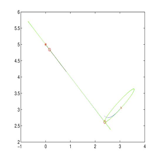
Figure 1: Arc-search for the simple example.

The feasible and infeasible central paths are arcs in $5$-dimensional space $(\lambda,x_{1},s_{1},x_{2},s_{2})$. If we project the central paths into $2$-dimensional subspace spanned by $(x_{1},x_{2})$, they are arcs in $2$-dimensional subspace. Figure 1 shows the first two iterations of Algorithm 3.1 in the $2$-dimensional subspace spanned by $(x_{1},x_{2})$. In Figure 1, the initial point $(x_{1}^{0},x_{2}^{0})$ is marked by ’x’ in red; the optimal solution is marked by ’*’ in red; $(\dot{x},\dot{s},\dot{\lambda})$ is calculated by using (12); $(\ddot{x},\ddot{s},\ddot{\lambda})$ is calculated by using (14); the projected feasible central path ${\cal C}(t)$ near the optimal solution is calculated by using (62) and is plotted as a continuous line in black; the infeasible central path ${\cal H}(t)$ starting from current iterate is calculated by using (9) and plotted as the dotted lines in blue; and the projected ellipsoidal approximations ${\cal E}(\alpha)$ are the dotted lines in green (they may look like continuous line some times because many dots are used). In the first iteration, the iterate ’x’ moves along the ellipse (defined by in Theorem 20) to reach the next iterate marked as ’o’ in red because the calculation of infeasible central path (the blue line) is very expensive and ellipse is cheap to calculate and a better approximation to the infeasible central path than a straight line. The rest iterations are simply the repetition of the process until it reaches the optimal solution $(s^{*},x^{*})$. Only two iterations are plotted in Figure 1.

It is worthwhile to note that in this simple problem, the infeasible central path has a sharp turn in the first iteration which may happen a number of times for general problem as discussed in [38]. The arc-search method is expected to perform better than Mehrotra’s method in iterations that are close to the sharp turns. In this simple problem, after the first iteration, the feasible central path ${\cal C}(t)$, the infeasible central path ${\cal H}(t)$, and the ellipse ${\cal E}(\alpha)$ are all very close to each other and close to a straight line.

5.2 Netlib test examples

The algorithm developed in this paper is implemented in a Matlab function. Mehrotra’s algorithm is also implemented in a Matlab function. They are almost identical. Both algorithms use exactly the same initial point, the same stopping criteria, the same pre-process, and the same parameters. The only difference of the two implementations is that arc-search method searches optimizer along an ellipse and Mehrotra’s method searches optimizer along a straight line. Numerical tests for both algorithms have been performed for all Netlib LP problems that are presented in standard form. The iteration numbers used to solve these problems are listed in Table 1. Only one Netlib problem Osa_60 ($m=10281$ and $n=232966$) presented in standard form is not included in the test because the PC computer used for the testing does not have enough memory to handle this problem.

Table 1: Numerical results for test problems in Netlib

Problem	before prep		after prep		Arc-search			Mehrotra
	m	n	m	n	iter	objective	infeas	iter	objective	infeas
Adlittle	56	138	54	136	15	2.2549e+05	1.0e-07	15	2.2549e+05	3.4e-08
Afiro	27	51	8	32	9	-464.7531	1.0e-11	9	-464.7531	8.0e-12
Agg	488	615	391	479	18	-3.5992e+07	5.0e-06	22	-3.5992e+07	5.2e-05
Agg2	516	758	514	755	18	-2.0239e+07	4.6e-07	20	-2.0239e+07	5.2e-07
Agg3	516	758	514	755	17	1.0312e+07	3.1e-08	18	1.0312e+07	8.8e-09
Bandm	305	472	192	347	19	-158.6280	3.2e-11	22	-158.6280	8.3e-10
Beaconfd	173	295	57	147	10	3.3592e+04	1.4e-12	11	3.3592e+04	1.4e-10
Blend	74	114	49	89	12	-30.8121	1.0e-09	14	-30.8122	4.9e-11
Bnl1	643	1586	429	1314	32	1.9776e+03	2.7e-09	35	1.9776e+03	3.4e-09
Bnl2	2324	4486	1007	3066	32	1.8112e+03	5.4e-10	37	1.8112e+03	9.3e-07
Brandy	220	303	113	218	20	1.5185e+03	3.0e-06	19	1.5185e+03	6.2e-08
Degen2*	444	757	440	753	16	-1.4352e+03	1.9e-08	17	-1.4352e+03	2.0e-10
Degen3*	1503	2604	1490	2591	22	-9.8729e+02	7.0e-05	22	-9.8729e+02	1.2e-09
fffff800	525	1208	487	991	26	5.5568e+005	4.3e-05	31	5.5568e+05	7.7e-04
Israel	174	316	174	316	23	-8.9664e+05	7.4e-08	29	-8.9665e+05	1.8e-08
Lotfi	153	366	113	326	14	-25.2647	3.5e-10	18	-25.2647	2.7e-07
Maros_r7	3136	9408	2152	7440	18	1.4972e+06	1.6e-08	21	1.4972e+06	6.4e-09
Osa_07*	1118	25067	1081	25030	37	5.3574e+05	4.2e-07	35	5.3578e+05	1.5e-07
Osa_14	2337	54797	2300	54760	35	1.1065e+06	2.0e-09	37	1.1065e+06	3.0e-08
Osa_30	4350	104374	4313	104337	32	2.1421e+06	1.0e-08	36	2.1421e+06	1.3e-08
Qap12	3192	8856	3048	8712	22	5.2289e+02	1.9e-08	24	5.2289e+02	6.2e-09
Qap15*	6330	22275	6105	22050	27	1.0411e+03	3.9e-07	44	1.0410e+03	1.5e-05
Qap8*	912	1632	848	1568	12	2.0350e+02	1.2e-12	13	2.0350e+02	7.1e-09
Sc105	105	163	44	102	10	-52.2021	3.8e-12	11	-52.2021	9.8e-11
Sc205	205	317	89	201	13	-52.2021	3.7e-10	12	-52.2021	8.8e-11
Sc50a	50	78	19	47	10	-64.5751	3.4e-12	9	-64.5751	8.3e-08
Sc50b	50	78	14	42	8	-70.0000	1.0e-10	8	-70.0000	9.1e-07
Scagr25	471	671	343	543	19	-1.4753e+07	5.0e-07	18	-1.4753e+07	4.6e-09
Scagr7	129	185	91	147	15	-2.3314e+06	2.7e-09	17	-2.3314e+06	1.1e-07
Scfxm1+	330	600	238	500	20	1.8417e+04	3.1e-07	21	1.8417e+04	1.6e-08
Scfxm2	660	1200	479	1003	23	3.6660e+04	2.3e-06	26	3.6660e+04	2.6e-08
Scfxm3+	990	1800	720	1506	24	5.4901e+04	1.9e-06	23	5.4901e+04	9.8e-08
Scrs8	490	1275	115	893	23	9.0430e+02	1.2e-11	30	9.0430e+02	1.8e-10
Scsd1	77	760	77	760	12	8.6666	1.0e-10	13	8.6666	8.7e-14
Scsd6	147	1350	147	1350	14	50.5000	1.5e-13	16	50.5000	7.9e-13
Scsd8	397	2750	397	2750	13	9.0500e+02	6.7e-10	14	9.0500e+02	1.3e-10
Sctap1	300	660	284	644	20	1.4122e+03	2.6e-10	24	1.4123e+03	2.1e-09
Sctap2	1090	2500	1033	2443	20	1.7248e+03	2.1e-10	21	1.7248e+03	4.4e-07
Sctap3	1480	3340	1408	3268	20	1.4240e+03	5.7e-08	22	1.4240e+03	5.9e-07
Share1b	117	253	102	238	22	-7.6589e+04	6.5e-08	25	-7.6589e+04	1.5e-06
Share2b	96	162	87	153	13	-4.1573e+02	4.9e-11	15	-4.1573e+02	7.9e-10
Ship04l	402	2166	292	1905	17	1.7933e+06	5.2e-11	18	1.7933e+06	2.9e-11
Ship04s	402	1506	216	1281	17	1.7987e+06	2.2e-11	20	1.7987e+06	4.5e-09
Ship08l**	778	4363	470	3121	18	1.9090e+06	1.6e-07	20	1.9091e+06	1.0e-10
Ship08s+	778	2467	274	1600	17	1.9201e+06	3.7e-08	19	1.9201e+06	4.5e-12
Ship12l*	1151	5533	610	4171	19	1.4702e+06	4.7e-13	20	1.4702e+06	1.0e-08
Ship12s+	1151	2869	340	1943	17	1.4892e+06	1.0e-10	19	1.4892e+06	2.1e-13
Stocfor1*	117	165	34	82	14	-4.1132e+04	2.8e-10	15	-4.1132e+04	1.1e-10
Stocfor2	2157	3045	766	1654	22	-3.9024e+04	2.1e-09	22	-3.9024e+04	1.6e-09
Stocfor3	16675	23541	5974	12840	34	-3.9976e+04	4.7e-08	38	-3.9976e+04	6.4e-08
Truss	1000	8806	1000	8806	22	4.5882e+05	1.7e-07	36	4.5882e+05	9.5e-06

Several problems have degenerate solutions which make them difficult to solve or need significantly more iterations. We choose to use the option described in Section 4.6 to solve these problems. For problems marked with ’+’, this option is called only for Mehrotra’s method. For problems marked with ’*’, both algorithms need to call this option for better results. For the problem with ’**’, in addition to call this option, the default value of $10^{-6}$ has to be changed to $10^{-4}$ for Mehrotra’s method. We need to keep in mind that although using the option described in Section 4.6 reduces the iteration count significantly, these iterations are significantly more expensive. Therefore, simply comparing iteration counts for problem(s) marked with ’+’ will lead to a conclusion in favor of Mehrotra’s method (which is what we will do in the following discussions).

Since the major cost in each iteration for both algorithms are solving linear systems of equations, which are identical in these two algorithms, we conclude that iteration numbers is a good measure of efficiency. In view of Table 1, it is clear that Algorithm 3.1 uses less iterations than Mehrotra’s algorithm to find the optimal solutions for majority tested problems. Among $51$ tested problems, Mehrotra’s method uses fewer iterations ($7$ iterations in total) than arc-search method for only $6$ problems (brandy, osa_07, sc205, sc50a, scagr25, scfxm3), while arc-search method uses fewer iterations ($126$ iterations in total) than Mehrotra’s method for $40$ problems. For the rest $5$ problems, both methods use the same number of iterations. Arc-search method is numerically more stable than Mehrotra’s method because for problems scfxm1, scfxm3, ship08s, ship12s, arc-search method does not need to use the option described in Section 4.6 but Mehrotra’s method need to use the option to solve the problems. For problem ship08l, Mehrotra’s method need to adjust parameter in the option to find the optimizer but arc-search method does not need to adjust the parameter.

6 Conclusions

This paper proposes an arc-search interior-point path-following algorithm that searches optimizers along the ellipse that approximate infeasible central path. The proposed algorithm is different from Mehrotra’s method only in search path. Both arc-search method and Mehrotra’s method are implemented in Matlab so that the two methods use exactly same initial point, the same pre-process, the same parameters, and the same stopping criteria. By doing this, we can compare both algorithms in a fair and controlled way. Numerical test is conducted for Netlib problems for both methods. The results show that the proposed arc-search method is more efficient and reliable than the well-known Mehrotra’s method.

7 Acknowledgments

The author would like to thank Mr. Mike Case, the Director of the Division of Engineering in the Office of Research at US NRC, and Dr. Chris Hoxie, in the Office of Research at US NRC, for their providing computational environment for this research.

References

- [1] S. Wright, Primal-Dual Interior-Point Methods, SIAM, Philadelphia, 1997.
- [2] N. Megiddo, Pathway to the optimal set in linear propramming, in Program in Mathematical Programming: interior point and related methods, N. Megiddo, ed., Springer Verlag, New York, (1989), pp. 131-158.
- [3] M. Kojima, S. Mizuno, and A. Yoshise, A polynomial-time algorithm for a class of linear complementarity problem, Mathematical Programming, 44, (1989), pp. 1-26.
- [4] M. Kojima, S. Mizuno, and A. Yoshise, A primal-dual interior point algorithm for linear programming, in Progress in Mathematical Programming: Interior-point and Related Methods, N. Megiddo, ed., Springer-Verlag, New York, 1989.
- [5] S. Mehrotra, On the implementation of a primal-dual interior point method, SIAM Journal on Optimization, 2, (1992), pp. 575-601.
- [6] I. Lustig, R. Marsten, and D. Shannon, Computational experience with a primal-dual interior-point method for linear programming, Linear Algebra and Its Applications, 152, (1991), pp. 191-222.
- [7] I. Lustig, R. Marsten, and D. Shannon, On implementing Mehrotra’s predictor-corrector interior-point method for linear programming, SIAM Journal on Optimization, 2, (1992), pp. 432-449.
- [8] S. Mizuno, Polynomiality of the Kojima-Megiddo-Mizuno infeasible interior point algorithm for linear programming, Mathematical Programming, 67, (1994), pp. 109-119.
- [9] Y. Zhang, On the convergence of a class of infeasible-interior-point methods for the horizontal linear complementarity problem, SIAM Journal on Optimization, Vol.4, (1994), pp. 208-227.
- [10] S. Mizuno, M. Todd, and Y. Ye, On adaptive step primal-dual interior-point algorithms for linear programming, Mathematics of Operations Research, 18, (1993), pp. 964-981.
- [11] J. Miao, Two infeasible interior-point predictor-corrector algorithms for linear programming, SIAM Journal on Optimization, Vol. 6, (1996), pp. 587-599.
- [12] C. Roos, A full-Newton step infeasible interior-point algorithm for linear optimization, SIAM Journal on Optimization, Vol. 16(4), (2006), pp. 1110-1136.
- [13] M. Salahi, J. Peng, and T. Terlaky, On Mehrotra-Type Predictor-Corrector Algorithms, SIAM J. on Optimization, 18, (2007), pp. 1377-1397.
- [14] B. Kheirfam, K. Ahmadi, and F. Hasani, A modified full-Newton step infeasible interior-point algoirhm for linear optimization, Asia-Pacific Journal of Operational Research, Vol. 30, (2013), pp.11-23.
- [15] L. B. Winternitz A. L. Tits P.-A. Absil, Addressing Rank Degeneracy in Constraint-Reduced Interior-Point Methods for Linear Optimization, J Optim Theory Appl 160, (2014), pp. 127-157.
- [16] R.J. Vanderbei. LOQO: An interior point code for quadratic programming. Optimization Methods and Software, (1999), 12:451 484.
- [17] J. Czyzyk, S. Mehrotra, M. Wagner, and S. J. Wright, PCx User Guide (version 1.1), Technical Report OTC 96/01, Optimization Technology Center, 1997.
- [18] Y. Zhang, Solving large-scale linear programs by interior-point methods under the matlab environment, Technical Report TR96-01, Department of Mathematics and Statistics, University of Maryland, 1996.
- [19] R. Monteiro, I. Adler, and M. Resende, A polynomial-time primal-dual affine scaling algorithm for linear and convex quadratic programming and its power series extension, Mathematics of Operations Research, 15, (1990), pp. 191-214.
- [20] C. Cartis, Some disadvantages of a Mehrotra-type primal-dual corrector interior point algorithm for linear programming, Applied Numerical Mathematics, 59, (2009), pp. 1110-1119.
- [21] Y. Yang, A Polynomial Arc-Search Interior-Point Algorithm for Linear Programming, Journal of Optimization Theory and Applications, Vol. 158, (2013), pp. 859-873.
- [22] Y. Yang, A polynomial arc-search interior-point algorithm for convex quadratic programming, European Journal of Operational Research, Vol. 215, (2011), pp. 25-38.
- [23] C. Cartis and N.I.M. Gould, Finding a point in the relative interior of a polyhedron, Technical Report NA-07/01, Computing Laboratory, Oxford University, 2007.
- [24] M. P. Do Carmo, Differential Geometry of Curves and Surfaces, Prentice-Hall, New Jersey, 1976.
- [25] A.L. Brearley, G. Mitra, and H.P. Williams, Analysis of methematical programming problems prior to applying the simplex algorithm, Mathematical Programming, 8, (1975), pp. 54-83.
- [26] E.D. Andersen and K. D. Andersen, Presolving in linear programming, Mathematical Programming, 71, (1993), pp. 221-245.
- [27] A. Mahajan, Presolving mixed-integer linear programs, Preprint ANL/MCS-P1752-0510, Argonne National Laboratory, 2010.
- [28] C. T.L.S. Ghidini, , A.R.L. Oliveira, Jair Silvab, and M.I. Velazco, Combining a hybrid preconditioner and a optimal adjustment algorithm to accelerate the convergence of interior point methods, Linear Algebra and its Applications Vol. 436, (2012), pp.1267-1284.
- [29] A.R. Curtis and J.K. Reid, On the automatic scaling of matrices for Gaussian elimination, J. Inst. Maths Applics, Vol. 10, (1972), pp. 118-124.
- [30] E.D. Andersen, Finding all linearly dependent rows in large-scale linear programming, Optimization Methods and Software, Vol. 6, (1995), pp. 219-227.
- [31] J.F. Duff, A.M. Erisman, and J.K. Reid, Direct method for sparse matrices, Oxford University Press, New York, 1989.
- [32] J. Dobes, A modified Markowitz criterion for the fast modes of the LU factorization. Proceedings of 48th Midwest Symposium on Circuits and Systems, (2005), pp. 955-959.
- [33] E. Ng and B.W. Peyton, Block sparse Cholesky algorithm on advanced uniprocessor computers, SIAM Journal on Scientific Computing, 14, (1993), pp. 1034-1056.
- [34] J.W. Liu, Modification of the minimum degree algorithm by multiple elimination, ACM Transactions on Mathematical Software, 11, (1985), pp.141-153.
- [35] A.J. Goldman and A.W. Tucker, Theory of linear programming, Linear Equalities and Related Systems, eds., H.W. Kuhn and Tucker, Princeton University Press, Princeton, N.J, (1956), pp.53-97.
- [36] O. Guler, D. den Hertog, C. Roos, T. Terlaky and Tsuchiya, Degeneracy in interior-point methods for linear programming: a survey, Annals of Operations Research, 46, (1993), pp. 107-138.
- [37] P.E. Gill, W. Murray, M.A. Saunders, J.A. Tomlin, and M.H. Wright, On projected Newton barrier methods for linear programming and an equivalence of Karmarkar’s projective method, Mathematical Programming, Vol. 36, (1986), pp. 183-209.
- [38] S. A. Vavasis and Y. Ye, A primal dual interior-point method whose running time depends on the constraint matrix, Mathematical Programming A, Vol. 74, (1996), pp.79-120.