Probing the $\nu=2/3$ fractional quantum Hall edge by momentum-resolved tunneling

Abstract

The nature of the fractional quantum Hall state with filling factor $\nu=2/3$ and its edge modes continues to remain an open problem in low-dimensional condensed matter physics. Here, we suggest an experimental setting to probe the $\nu=2/3$ edge by tunnel-coupling it to a $\nu=1$ integer quantum Hall edge in another layer of a two-dimensional electron gas (2DEG). In this double-layer geometry, the momentum of tunneling electrons may be boosted by an auxiliary magnetic field parallel to the two planes of 2DEGs. The threshold behavior of the current as a function of bias voltage and the boosting magnetic field yields information about the spectral function of the $\nu=2/3$ edge, and in particular about the nature of the chiral edge modes. Our theoretical analysis accounts also for the effects of Coulomb interaction and disorder.

Introduction.

In the conditions of quantum Hall effect, the compressible regions remain only at the edges of a sample and are known as edge states [1, 2]. Edges of fractional Hall states are strongly-correlated chiral electron liquids [3]. The situation becomes even more intriguing for systems with filling factors different from those of Laughlin states, for which $\nu=1/m$ with odd integer $m>0$. Here we consider the particular case of a quantum Hall system with filling factor $\nu=2/3$.

A prominent conjecture [4, 5] considers the $\nu=2/3$ edge [6, 7] as composed of two spatially separated edge channels: an outer channel with filling factor $\nu=1$ and an inner counter-propagating one corresponding to a $\nu=1/3$ liquid of hole states. Coulomb interactions between the two channels and backscattering off disorder enrich the physical picture and in the low-energy limit drive the system into a state with universal two-terminal and Hall conductance $G=2e^{2}/3h$ [8]. Theory [8] predicts two effective edge modes, a charge-carrying mode and a counter-propagating neutral one. Recent shot noise measurements at a quantum point contact [9] have provided indirect evidence for the existence of such a neutral mode and a mechanism of upstream heating by neutral currents [9, 10, 11]. However, two observations put the picture of two counter-propagating modes in question and favor the possibility of two co-propagating $\nu=1/3$ modes as alternatively suggested long ago [12]. One is the observation of a $G=e^{2}/3h$ plateau [13, 14] in the conductance through quantum point contacts. The second is the effective charge, detected through shot noise measurements [14], which crosses over from $e/3$ at higher temperature to $2e/3$ at lower ones. A “unified” theory has recently [15] been proposed in terms of a four-channel model for a reconstructed edge. In this situation of competing theories, direct experimental evidence about the internal structure of the $\nu=2/3$ edge is called for.

In this paper, we are suggesting a bilayer experiment to investigate the spectral function and, in particular, the nature of the chiral modes of the $\nu=2/3$ edge. In this experiment, the fractional quantum Hall edge is probed by momentum-resolved tunneling into or from the edge of an integer quantum Hall state with filling factor $\nu=1$, which we understand rather well. Applying an in-plane magnetic field $B_{y}$ allows one to extract the spectral function upon measuring the current $I$ as a function of $B_{y}$ and bias voltage $V$ in a two-terminal setting. We show how the geometry of the edge channels corresponds in the $V$–$B_{y}$ plane to a pattern of equidistant valleys of current $I$, where lines of non-analyticity with exponents characteristic to the filling factor intersect.

The suggested experiment on the $\nu=2/3$ edge is inspired by experiments on tunnel-coupled parallel quantum wires [16]. In the latter setup, measuring the tunnel current as a function of bias voltage and a transverse magnetic field provided direct information about the threshold lines (in energy–momentum space) for the spectral function and, hence, about the velocities of the spin and charge modes of the one-dimensional electron liquid [17]. In the context of the quantum Hall effect, similar settings using momentum-conserved tunneling have been discussed in Refs. [18, 19, 20, 21]. Bilayer settings like the one we are suggesting are to be distinguished from tunnel-coupled lateral quantum Hall systems [22].

Setting.

Figure 1 presents the double-layer layout we suggest for probing the $\nu=2/3$ state. Each layer contains a 2DEG with suitable individual gating and doping such that the magnetic field $B_{z}$ establishes a $\nu=2/3$ state in the lower layer and a $\nu=1$ state in the upper one. The distance $d$ between the layers is chosen such that the layers are coupled via electron tunneling. The specific feature of our setting is that the edges of the two quantum Hall states are aligned on top of each other. This may be achieved by applying voltages to a top-right gate and a bottom-left gate that deplete the right part of the upper and the left part of the lower 2DEG. Full depletion of one layer’s halfplane without affecting the other layer is possible for screening lengths of the order of the Bohr radius, which in realistic experiments can be the case [23]. In the absence of quantum Hall features ($B_{z}=0$), momentum-resolved tunneling between two parallel 2DEGs was experimentally realized [24] for $d\approx 70\ \mathrm{\AA}$ and in-plane magnetic fields up to $B_{y}\sim 8\ \mathrm{T}$. Scanning over a width of the magnetic length $\ell_{B_{z}}=\sqrt{\hbar/eB_{z}}\sim 100\ \mathrm{\AA}$ requires fields $B_{y}$ up to $10\ \mathrm{T}$. In order to avoid such strong transverse fields, one may equivalently adjust the gate voltages to move the edges by $\Delta y$ [25], corresponding to a momentum boost $\hbar\Delta y/\ell_{B_{z}}^{2}$, and resort to a $B_{y}$ of smaller magnitude for fine-tuned momentum scans close to a valley.

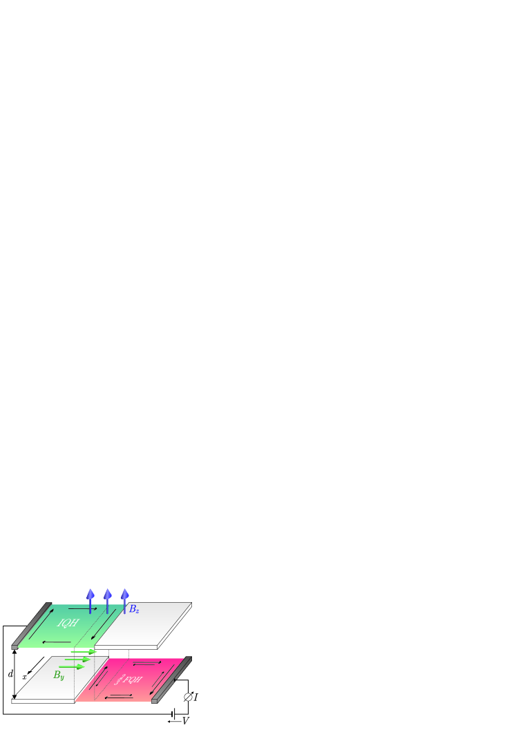
Figure 1: (Color online) Suggested experimental setup to study the $\nu=2/3$ fractional quantum Hall (FQH) edge. The tunnel current $I$ between the FQH edge and the probing $\nu=1$ integer quantum Hall (IQH) edge is measured as a function of bias voltage $V$ and transverse magnetic field $B_{y}$, which boosts the momentum of tunneling electrons by $Q=eB_{y}d$.

Model.

The upper integer quantum Hall edge, which serves to probe the $\nu=2/3$ edge, is described using a simple model of chiral electrons with spectrum $\varepsilon_{0,k}=u_{0}k-\varepsilon_{0}$ that propagate in a positive (upward) $x$-direction. For the $\nu=2/3$ edge, we adopt the low-energy fixed-point theory by Kane, Fisher, and Polchinski (KFP) [8] for a theoretical discussion of the suggested experiment. KFP assume in the bare picture an exterior downward-propagating $\nu=1$ and an inner upward-propagating $\nu=1/3$ edge channel [3, 4, 5] associated with bosonic fields $\phi_{1}(x)$ and $\phi_{2}(x)$, respectively. These satisfy the commutation relations $[\phi_{i}(x),\phi_{j}(x^{\prime})]=(\mathrm{i}\pi\delta_{ij}/K_{i})\ \mathrm{sgn}(x-x^{\prime})$ with $K_{1}=-1$ and $K_{2}=3$.

The clean $\nu=2/3$ edge is described by the Hamiltonian

$$\hat{H}_{2/3} =\int\frac{\mathrm{d}x}{4\pi}\ \big{[}u_{1}(\nabla\phi_{1})^{2}+3u_{2}(\nabla\phi_{2})^{2}+2u_{12}\nabla\phi_{1}\nabla\phi_{2}\big{]}\ .$$ (1)

We assume that velocities $u_{1}$ and $u_{2}$ have already been renormalized by intrachannel Coulomb interactions. If interchannel Coulomb interactions are absent ($u_{12}=0$), the Hamiltonians for the probing edge and the $\nu=2/3$ edge lead to the spectrum in Fig. 2. The spatial separation of the two channels inside the $\nu=2/3$ edge implies a (gauge-invariant) distance $\kappa$ between their Fermi points in canonical momentum space. It is determined by the chemical potential $\mu$, the field $B_{z}$ establishing the quantum Hall regime, and details of the edge potential.

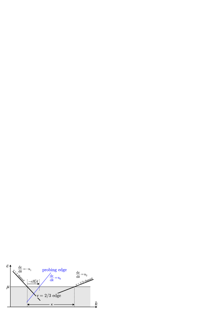
Figure 2: (Color online) Spectrum of the $\nu=2/3$ edge channels (solid lines) containing a branch for the outer downward-propagating $\nu=1$ channel and the the inner counter-propagating $\nu=1/3$ channel. The dashed blue line represents the edge of the probing $\nu=1$ integer quantum Hall edge of the upper layer.

At finite $u_{12}$, the independently propagating modes are given, instead of $\phi_{1,2}$, by $\phi_{+}=\sqrt{\eta-1}\phi_{1}+\sqrt{3\eta}\phi_{2}$ and $\phi_{-}=\sqrt{\eta}\phi_{1}+\sqrt{3(\eta-1)}\phi_{2}$, propagating with velocities $u_{\pm}=(u_{2}-u_{1})/2\pm(u_{1}+u_{2})\gamma/2$. Herein, $\eta=(1+\gamma)/2\gamma$, $\gamma=\sqrt{1-c^{2}}$, and $c=(2/\sqrt{3})\ u_{12}/(u_{1}+u_{2})$. The coefficient $\eta$ takes values between $\eta=1$ for $u_{12}=0$ and $\eta=3/2$ at the low-energy fixed point [8]. In terms of the effective modes,

$$\hat{H}_{2/3} =\int\frac{\mathrm{d}x}{4\pi}\ \big{[}-u_{-}(\nabla\phi_{-})^{2}+u_{+}(\nabla\phi_{+})^{2}\big{]}\ .$$ (2)

We assume $u_{+}<u_{0}$, consistent with slow neutral modes.

At the low-energy fixed point $\eta=3/2$, charge transport only involves $\phi_{-}$ whereas $\phi_{+}$ is a counter-propagating neutral mode [8]. Reaching this fixed point requires an equilibration mechanism such as backscattering off impurities. The most relevant Hamiltonian for interchannel backscattering reads

$$\hat{H}_{D} =\int\mathrm{d}x\ \xi(x)\ \exp\big{\{}-\mathrm{i}(\phi_{1}+3\phi_{2})\big{\}}+\mathrm{H.c.}$$ (3)

Herein, the operator $\exp(-\mathrm{i}\phi_{1})$ creates a quasi-particle of charge $-e$ in the outer channel while $\exp(-3\mathrm{i}\phi_{2})$ annihilates three quasi-particles, each of charge $-e/3$, in the inner channel. Following KFP, we assume Gaussian disorder, $\langle\xi(x)\xi^{*}(x^{\prime})\rangle=w\delta(x-x^{\prime})$. At $\eta=3/2$, $\hat{H}_{D}=\int\mathrm{d}x\ \xi(x)\exp(-\mathrm{i}\sqrt{2}\phi_{+})+\mathrm{H.c.}$, so only the neutral mode is affected.

Finally, we choose a proper model for interedge tunneling. We assume the barrier between the probing and fractional edge homogeneous, implying momentum-conserving tunneling at zero transverse field $B_{y}$. A finite $B_{y}$ boosts the momentum of the tunneling electron by $Q=eB_{y}d$. Assuming tunneling matrix elements $t_{0}\delta_{kk^{\prime}}$ in the space of canonical momentum $k$, we are led to the tunneling Hamiltonian

$$\hat{H}_{T} =t_{0}\sum_{k}\hat{\psi}^{\dagger}_{2/3,k}\hat{\psi}^{\phantom{\dagger}}_{0,k+Q}+\mathrm{H.c.}$$ (4)

Here $\hat{\psi}_{0}$ is the electron field operator for the probing edge. The most general field operator for the annihilation of charge $-e$ in the $\nu=2/3$ edge has the form

$$\hat{\psi}_{2/3}(x) =\frac{\mathrm{e}^{\mathrm{i}\phi_{1}(x)}}{(2\pi\alpha)^{1/2}}\sum_{n=-\infty}^{\infty}A_{n}\mathrm{e}^{\mathrm{i}n\kappa x}\mathrm{e}^{-\mathrm{i}n[\phi_{1}(x)+3\phi_{2}(x)]}$$ (5)

with amplitudes $A_{n}$ and ultraviolet length cutoff $\alpha$. If the channels were uncoupled, all $A_{n}$ would be zero except for $A_{0}$ and $A_{1}$. These two correspond to annihilation of charge $-e$ in the $\nu=1$ and $\nu=1/3$ channels, respectively. Terms different from these two additionally transfer integer multiples of charge $e$ between the two channels, thus generating dipole excitations. We assume $A_{n}\sim 1$ for all $n$ as is the case in a generic Luttinger liquid [17], where $\kappa$ is given by twice the Fermi momentum.

Kinematic picture.

Before delving into effects of disorder and interaction, let us discuss the kinematics of the setup in Fig. 1. A finite bias voltage $V$ effectively shifts both the spectrum and the chemical potential of the probing edge (Fig. 2) in vertical direction while a momentum boost by $B_{y}$ corresponds to a horizontal shift of the spectrum of the probing edge. There exists a unique value $B_{y}^{(0)}$ such that interlayer tunneling couples the Fermi momentum state of the probing edge to that of the $\nu=1$ channel in the fractional edge. Henceforth, we denote by $B_{y}$ the magnetic field measured from $B_{y}^{(0)}$. In $\hat{H}_{T}$, Eq. (4), this has already been assumed.

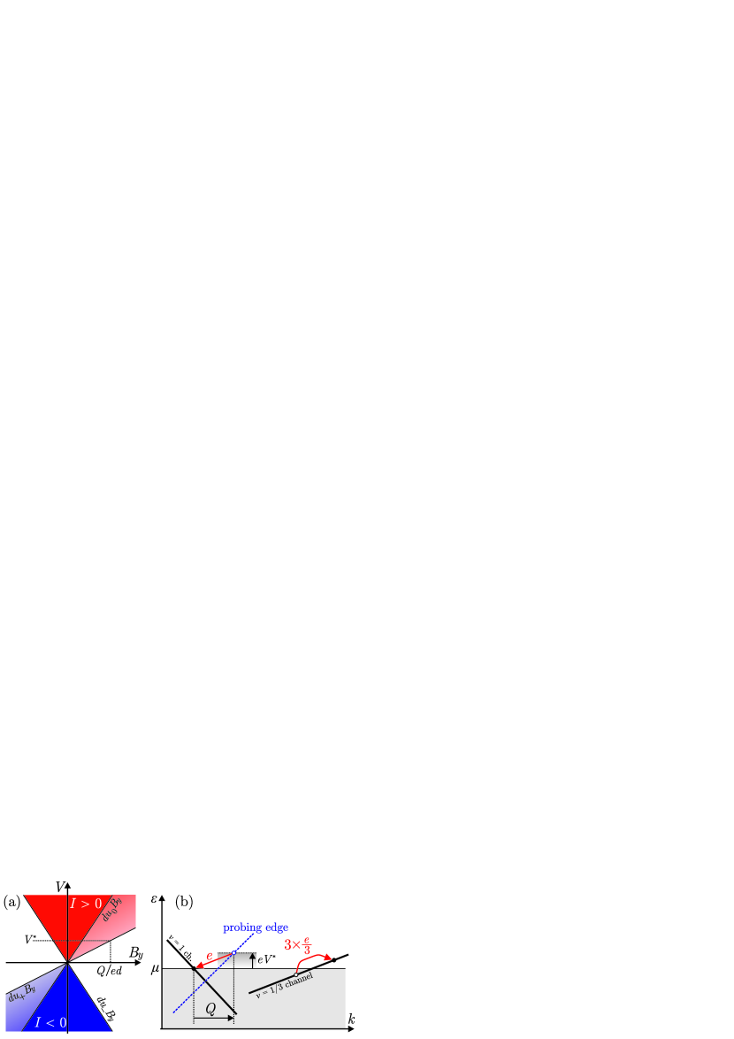
Figure 3: (Color online) Kinematic picture for tunneling between the probing edge and the $\nu=1$ channel of the $\nu=2/3$ edge. (a) Regions of non-zero tunnel current in the $B_{y}$–$V$ plane. (b) Interaction-induced tunneling at (positive) bias voltage $V^{*}=Qu_{+}/e$.

Neglecting interchannel Coulomb interactions, $u_{-}=-u_{1}$ and $u_{+}=u_{2}$. For small $Q=eB_{y}d$, the probing edge is close to the outer channel of the $\nu=2/3$ edge, and we need to retain only the term $n=0$ in the sum of Eq. (5). Momentum-resolved tunneling between the edges requires the intercept point $k_{\times}$ of the edge bands to correspond to an occupied state in the shifted probing edge ($\varepsilon_{0,Q+k_{\times}}<\mu+eV$) and to an empty one in the fractional quantum Hall edge ($\varepsilon_{1,k_{\times}}>\mu$) or vice versa. At zero temperature, this condition is met for pairs $(B_{y},V)$ in the dark-colored regions in Fig. 3(a) with boundaries defined by velocities $u_{-}$ and $u_{0}$. In these regions, Fermi’s golden rule yields a current per unit length of value $I=\pm et_{0}^{2}/(u_{0}+u_{1})$ (see Appendix A).

Consider now the bias voltage $V^{*}=Qu_{+}/e$ [Fig. 3(b)]. Clearly, $V^{*}$ is not strong enough for momentum-resolved tunneling as discussed above, yet imagine an electron at the Fermi point of the probing edge tunneling into the lowest unoccupied state of the nearby fractional quantum Hall edge channel. This violates momentum and energy conservation. But, since the quotient of energy and momentum mismatches equals the slope $u_{+}$ of the inner $\nu=1/3$ channel, an interaction-induced quasi-particle excitation in this inner channel can restore overall momentum and energy conservation. This Coulomb-supported tunneling works for voltages above $Qu_{+}/e$, annexing the light-colored zones in Fig. 3(a) to the regions of non-zero current, whose boundaries are thus determined solely by the spectrum of the $\nu=2/3$ edge.

Similar considerations at $Q\sim\kappa$ lead to another valley in the $B_{y}$–$V$ plane for tunneling between the probing edge and the $\nu=1/3$ channel, corresponding to the $A_{1}$ term in Eq. (5). Including all $A_{n}$ leads to a pattern of valleys situated at integer multiples of $\kappa$. The additional valleys are analogs to the “shadow bands” in one-dimensional systems [26]. We now turn to studying the current within the proper Luttinger-liquid formalism.

Current.

In linear-response theory with respect to interlayer electron tunneling $\hat{H}_{T}$, we obtain the tunnel current per unit length between the $\nu=2/3$ and the probing edge by expanding $I=-2et_{0}\sum_{k}\mathrm{Im}\langle\hat{\psi}^{\dagger}_{2/3,k}\hat{\psi}^{\phantom{\dagger}}_{0,k+Q}\rangle$ to order $t_{0}^{2}$. In the absence of disorder, the Luttinger-liquid formalism [27] then yields $I=\sum_{n=-\infty}^{\infty}|A_{n}|^{2}I_{n}$ with

$$I_{n} =\frac{et_{0}^{2}}{\pi^{2}}\int\mathrm{d}x\int_{-\infty}^{0}\mathrm{d}t\ \mathrm{Im}\Big{[}\frac{\sin(eVt-(Q-n\kappa)x)}{x-u_{0}t-\mathrm{i}\alpha}\ C_{n}(x,t)\Big{]}\ ,$$ (6)

where

$$C_{n}(x,t) =\frac{\alpha^{\mu^{+}_{n}+\mu^{-}_{n}-1}}{(x-u_{+}t-\mathrm{i}\alpha)^{\mu^{+}_{n}}(x-u_{-}t+\mathrm{i}\alpha)^{\mu^{-}_{n}}}$$ (7)

with valley-specific exponents $\mu^{\pm}_{n}$ is the zero-temperature correlation function for valley $n$. For valley $n$, e.g., $\mu^{+}_{0}=\eta-1$ and $\mu^{-}_{0}=\eta$. Letting $x=-tu$ [27], we readily integrate over time $t$. Studying the remaining integral over $u$, we identify regions of non-zero current and derive asymptotes for $eV$ close to $u_{\zeta}Q$ for $\zeta\in\{\pm,0\}$. Characteristic exponents resulting from such calculations (see Appendix A) are presented in the $I$-$V$ diagrams of Figs. 4(b) and (c) for the valleys $n=0$ and $1$. Numerical evaluation of Eq. (6) leads to the plot in Fig. 4(a) showing the first four valleys. The slopes of the non-analytic lines that limit the regions of non-zero current are determined by the velocities $u_{\pm}$ of the effective modes [Eq. (2)].

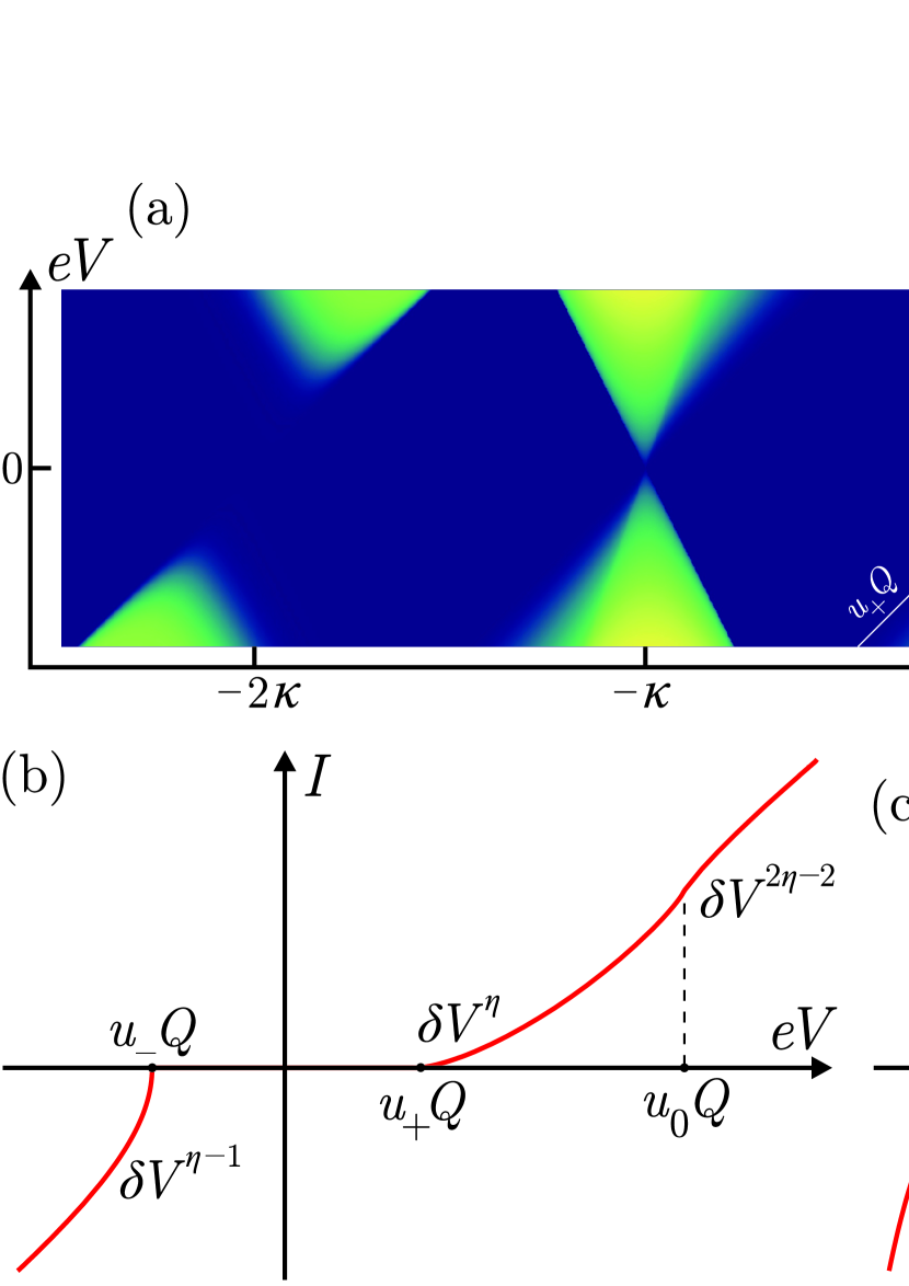
Figure 4: (Color online) (a) First four valleys for the current $I(V,Q)$ where $Q=eB_{y}d$. Coarse control of $Q$ on the scale of $\kappa$ is possible also by tuning the gate voltages. (b), (c) $I(V)$ curves for valleys $n=0$ and $1$ and asymptotic power laws close to non-analytic lines, $V=u_{\zeta}Q/e+\delta V$ where $\zeta\in\{\pm,0\}$. At $\eta=3/2$, the power law $\delta V^{2\eta-2}$ turns into $-\delta V\ln|\delta V|$.

In the universal limit $\eta=3/2$, the exponents in (7) for the valley at $n\kappa$ are given by the simple formulas $\mu^{+}_{n}=(2n+1)^{2}/2$ and $\mu^{-}_{n}=3/2$ [18]. The exponent $\mu^{+}_{n}$ of the non-analytic line defined by $u_{-}$ is smallest for $n=0$ and $-1$. These are the most relevant terms in $\hat{\psi}_{2/3}$ [Eq. (5)]. However, the exponent $\mu^{-}_{n}$, which describes the non-analytic behavior at the line defined by $u_{+}$, is $n$-independent. This in the context of Luttinger liquid theory [17] unusual feature of the spectral function is readily understood: Indeed, the number of excited charge modes of a summand in $\hat{\psi}_{2/3}$ does not depend on $n$, which counts neutral modes $\phi_{+}\propto\phi_{1}+3\phi_{2}$ only.

An exponent $\mu^{-}_{n}=3/2$, universal for all valleys, is reminiscent of the scaling $I\propto V^{1/\nu}$ seen [28] in tunneling from a lead into fractional quantum Hall layers regardless of $\nu$ not being a primary filling factor — an observation contrary to earlier theoretical predictions [29]. The point of view of momentum-conserving tunneling may thus open new possibilities in understanding the observation. In the experiment suggested here, the universality of $\mu^{-}_{n}$ may be smeared for large $n$ due to the increasing exponent at the nearby other non-analytic line and, in the presence of disorder, by scattering, whose effect on $I$ grows with $n$.

We note that other edge models [12, 15] would lead to patterns that differ from the one in Fig. 4. Specifically, the slopes of lines separating the bright (high-current) and dark regions as well as distances between bright regions are model-dependent; the same is true for the exponents $\mu_{n}$. The suggested experiment would thus distinguish between possible models.

Role of disorder.

For strong Coulomb interaction, backscattering off impurities [Eq. (3)] is a relevant perturbation in the renormalization group sense [30] and drives the $\nu=2/3$ quantum Hall layer to universal conductance $G=2e^{2}/3h$ at low energies [8]. In the following discussion, we already assume the low-energy fixed point and treat $l=2u_{+}^{2}/w$ as the effective mean free path [31].

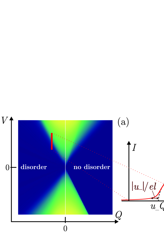
Figure 5: (Color online) (a) Current $I(V,Q)$ in the clean limit and for weak disorder. (b) $I(V)$ for $V$ close to $|u_{-}Q|$ in the presence and absence (dashed) of disorder.

Let us have a closer look at voltages $V=u_{-}Q/e+\delta V$ with small $\delta V$ in the valley $n=0$. Here the smallest exponent occurs ($\mu^{+}_{0}=1/2$). As long as disorder is weak compared to the boosting field, $l^{-1}\ll Q$, its effect is merely to blur the non-analytic lines in the current function $I(V,B_{y})$, see Fig. 5(a). In fact, since $Q\sim 10^{7}\ \mathrm{m}^{-1}[B_{y}/1\ \mathrm{T}]$ and since experimental evidence (e.g. [14]) indicates that $l$ should be at least $\sim 1\ \mu\mathrm{m}$, the assumption of weak disorder seems valid. Technically, disorder introduces in the correlation function $C_{0}(x,t)$, Eq. (7), a factor $\exp(-|x|/l)$ (see Appendix B). Close to the non-analytic line $eV=u_{\zeta}Q$, however, an explicit evaluation of $I(V)$ is still possible (see Appendix A). Along the vertical bar in Fig. 5(a),

$$I(\delta V)\simeq\frac{4et_{0}^{2}\alpha|u_{-}|^{\frac{1}{2}}}{\pi(u_{0}-u_{-})(u_{+}-u_{-})^{\frac{1}{2}}}\frac{|Q|^{\frac{1}{2}}}{l^{\frac{1}{2}}}\ g\Big{(}\frac{\delta V}{|u_{-}|/el}\Big{)}\ .$$ (8)

The shape of the blurring [see Fig. 5(b)] is described by the function $g(x)=-\mathrm{Im}[(-x-\mathrm{i})^{1/2}]$. For $x\gg 1$, $g(x)\simeq\sqrt{x}$, restoring the $I\propto\delta V^{1/2}$ power law of the clean edge at large bias voltage. For $x\rightarrow-\infty$, $g(x)\simeq(-x)^{-1/2}/2$ and we find a power law decay $I\propto l^{-1}(-\delta V)^{-1/2}$ at bias voltages below $|u_{-}Q|$. In the clean limit, $l\rightarrow\infty$, we recover $I=0$ for $\delta V<0$. Finally, as shown in Fig. 5(b), the function $I(V)$ in the presence of disorder is slightly displaced in the positive $V$-direction. This shift $\sim(|u_{-}|/e)(l^{3}|Q|)^{-1/2}$ is a next-to-leading order correction to formula (8).

Conclusion.

We have suggested a bilayer experimental setup to study the spectral function of the $\nu=2/3$ state in a two-terminal measurement of current as a function of bias voltage and transverse magnetic field. The edge model of two counter-propagating channels may be tested by its predicted pattern of current valleys. We studied the non-analyticities in the current-voltage characteristics associated with the channels, finding universal exponents. Discussing the role of disorder, we quantified its blurring effect for the non-analytical features of the current found here.

Acknowledgments.

We thank I. Petković for discussions. This work was supported by the U.S.-Israel Binational Science Foundation (Grant 2010366), by NSF DMR-1206612, by the German-Israeli Foundation (GIF), and by the DFG. H.M. acknowledges the Yale Prize Postdoctoral Fellowship.

I Appendix A: Calculation of tunnel current

In this Appendix, we present the explicit evaluation of the tunnel current in the absence and presence of disorder. We consider here only the $n=0$ term in the field operator $\hat{\psi}_{2/3}$ [Eq. (5)], corresponding to tunneling between the probing edge and the $\nu=1$ channel of the fractional edge without exciting additional neutral modes. We are going to focus on bias voltages $V=(u_{-}+\delta u)Q/e$ (where $Q=eB_{y}d$) mostly in the limit of small $\delta u$, i.e. $|\delta u|\ll|u_{-}|,u_{+}$. We remind the reader that $u_{-}<0$.

I.1 Free chiral electrons

As a warm-up exercise, we consider tunneling between the probing edge and the $\nu=1$ channel of the $\nu=2/3$ edge in the absence of both disorder and Coulomb interactions, $u_{12}=0$. Then, clearly, $u_{+}=u_{2}$ and $u_{-}=-u_{1}$. In the limit of non-interacting free electrons, we straightforwardly obtain the current per unit length $I$ using Fermi’s golden rule,

$$I =\frac{2\pi e}{L}\sum_{k,k^{\prime}}|t_{kk^{\prime}}|^{2}\delta(-u_{1}(k-Q)-u_{0}k+eV)\big{\{}f(-u_{1}(k-Q))\big{[}1-f(u_{0}k)\big{]}-\big{[}1-f(-u_{1}(k-Q))\big{]}f(u_{0}k)\big{\}}\ ,$$ (9)

where $L$ is the length of the tunnel-coupled edges, $t_{kk^{\prime}}$ the tunneling matrix element, and $f(\varepsilon)=[\exp(\varepsilon/T)+1]^{-1}$ the Fermi distribution function. For momentum-resolved tunneling, $t_{kk^{\prime}}=t_{0}\delta_{kk^{\prime}}$, cf. Eq. (4). In the zero-temperature limit $T\rightarrow 0$, the evaluation of the then trivial integrals in Eq. (9) yields

$$I =\frac{et_{0}^{2}}{u_{0}+u_{1}}\big{[}\Theta(eV-u_{0}Q)-\Theta(-eV-u_{1}Q)\big{]}\ .$$ (10)

In this formula, $\Theta$ denotes the Heaviside step function. Plotting $I$, Eq. (10), as a function of $V$ and $B_{y}$ leads to the two dark-colored regions in Fig. 3(a) with constant non-zero current $I=et_{0}^{2}/(u_{0}+u_{1})$ for $V>0$ and $I=-et_{0}^{2}/(u_{0}+u_{1})$ for $V<0$.

I.2 Strongly-correlated edge

Let us now turn to the physically more realistic model of the strongly-correlated $\nu=2/3$ edge as studied in Ref. [8]. For simplicity, we assume transverse magnetic fields $B_{y}$ such that $Q>0$. We thus start with the following expression for the current $I=I_{0}$, cf. Eq. (6):

$$I =\frac{t_{0}^{2}\alpha^{2\eta-2}}{\pi^{2}}\int_{-\infty}^{0}\mathrm{d}t\int\mathrm{d}x\sin(eVt-Qx)\exp(-|x|/l)\ \mathrm{Im}\Big{[}\frac{1}{(x-u_{0}t-\mathrm{i}\alpha)(x-u_{+}t-\mathrm{i}\alpha)^{\eta-1}(x-u_{-}t+\mathrm{i}\alpha)^{\eta}}\Big{]}\ .$$ (11)

The factor $\exp(-|x|/l)$ is due to disorder. We present a derivation of it starting from the microscopic model used in the main text in Appendix B. In the clean limit, $l\rightarrow\infty$ and this factor becomes unity. Transforming the spatial variable as $x=-tu$ and $\mathrm{d}x=-t\mathrm{d}u$ [27], we are in the position to immediately perform the integration over time $t$. We obtain

$$I =\frac{t_{0}^{2}\alpha^{2\eta-2}Q^{2\eta-2}}{\pi^{2}}\int\mathrm{d}u\ \Gamma(2-2\eta)\ \mathrm{Im}\Big{[}\frac{\mathrm{i}}{2}\frac{\mathrm{e}^{\mathrm{i}\pi\eta}(u_{-}+\delta u+u-\mathrm{i}\varepsilon|u|)^{2\eta-2}-\mathrm{e}^{-\mathrm{i}\pi\eta}(u_{-}+\delta u+u+\mathrm{i}\varepsilon|u|)^{2\eta-2}}{(u+u_{0}-\mathrm{i}\tilde{\alpha})(u+u_{+}-\mathrm{i}\tilde{\alpha})^{\eta-1}(u+u_{-}+\mathrm{i}\tilde{\alpha})^{\eta}}\Big{]}$$ (12)

with $\varepsilon=1/(lQ)$ and $\tilde{\alpha}\rightarrow 0^{+}$.

I.3 Clean limit

In the clean limit, $l\rightarrow\infty$ (or $\varepsilon\rightarrow 0$) and Eq. (12) reduces to

$$I =-\frac{t_{0}^{2}\alpha^{2\eta-2}Q^{2\eta-2}}{\pi^{2}}\sin(\pi\eta)\int\mathrm{d}u\ \Gamma(2-2\eta)\ \mathrm{Im}\Big{[}\frac{\mathrm{sgn}(u_{-}+\delta u+u)|u_{-}+\delta u+u|^{2\eta-2}}{(u+u_{0}-\mathrm{i}\tilde{\alpha})(u+u_{+}-\mathrm{i}\tilde{\alpha})^{\eta-1}(u+u_{-}+\mathrm{i}\tilde{\alpha})^{\eta}}\Big{]}\ .$$ (13)

The integration contour of the integral (13) lies between two branch cuts, see Fig. 6(a). Poles of order $\geq 1$ are at $-u_{0}+\mathrm{i}\tilde{\alpha}$ and $-u_{-}-\mathrm{i}\tilde{\alpha}$, another pole of order $<1$ is found at $-u_{+}+\mathrm{i}\tilde{\alpha}$. The numerator introduces a non-analyticity at $u=-u_{-}-\delta u$. We evaluate the integral separately for the two cases $\delta u>0$ and $\delta u<0$. In the following, we interpret for each step the order of integration over $u$ and taking the imaginary part in the way as it is more convenient, since these two operations commute.

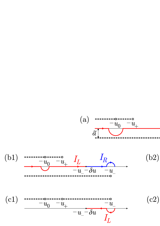
Figure 6: (a) Contour of integration in Eq. (13). For $u>-u_{-}$, the imaginary part and, hence, the integrand vanishes. For $\delta u>0$, (b1) shows the decomposition of the integration contour into the two sub-contours for integrals $I_{L}$ and $I_{R}$ along which the argument of $\mathrm{Im}$ is analytic; (c1) shows the deformed integration contour of the “reorganized” integrand of Eq. (14). One finds that $I_{L}$ and $I_{R}$ cancel each other. For $\delta V<0$, (b2) shows a convenient decomposition of the integral $I$, whose left part $I_{L}$ is similarly “reorganized”. The contour of $I_{L}$ is then deformed as shown in (c2). $I_{R}$ and $I_{L}$ together produce the finite contribution to the current given in Eq. (16).

Case $\delta u>0$.

In the case $\delta u>0$, we cut the integration contour at the non-analytic point $u=-u_{-}-\delta u<-u_{-}$ into a left ($L$) and right ($R$) part, see Fig. 6(b1). For the left part, we “reorganize” the integrand as

$$I_{L} =\frac{t_{0}^{2}\alpha^{2\eta-2}Q^{2\eta-2}}{\pi^{2}}\sin(\pi\eta)\int_{-\infty}^{-u_{-}-\delta u}\mathrm{d}u\ \Gamma(2-2\eta)\ \mathrm{Im}\Big{[}\frac{(u_{-}+\delta u+u-\mathrm{i}\tilde{\alpha})^{2\eta-2}}{(u+u_{0}-\mathrm{i}\tilde{\alpha})(u+u_{+}-\mathrm{i}\tilde{\alpha})^{\eta-1}(u+u_{-}-\mathrm{i}\tilde{\alpha})^{\eta}}\Big{]}\ .$$ (14)

In the form of Eq. (14), all poles and branch cuts are located in the upper half-plane and we may deform the contour as shown in Fig. 6(c1). Investigating $I_{L}$ along the new contour, we quickly recognize that $I_{L}=-I_{R}$ so that for $\delta u>0$, we find

$$I(\delta u>0)=0\ .$$ (15)

Note that this holds for all $\delta u$ with $0<\delta u<u_{+}-u_{-}$, independently from whether $\delta u$ is small.

Case $\delta u<0$.

In the case $\delta u<0$, the non-analyticity of the numerator lies to the right of $-u_{-}$. We thus split the integration contour at $u=-u_{-}-\rho$ with $\rho\rightarrow 0$ the radius of the semi-circle around the pole at $-u_{-}$, see Fig. 6(b2). For the left part, we reorganize the poles as in Eq. (14) and deform the integration contour as in Fig. 6(c2). Contrarily to the case $\delta u>0$, there is evidently no cancellation of $I_{L}$ and $I_{R}$. We calculate $I_{R}$ and $I_{L}$ in the limit of small $\delta u$ separately for finite $\rho$, leading to two divergent contributions in the limit $\rho\rightarrow 0$. The sum $I_{L}+I_{R}$, however, is regular as it should be, and reexpressing $\delta u$ in terms of a small (negative) voltage $\delta V=Q\delta u/e$, we find

$$I(\delta V) \simeq-\frac{C_{-}et_{0}^{2}\alpha^{2\eta-2}}{(u_{0}-u_{-})(u_{+}-u_{-})^{\eta-1}}Q^{\eta-1}(-e\delta V)^{\eta-1}$$ (16)

with $C_{-}=4^{\eta-1}\Gamma(\eta-\tfrac{1}{2})/(\pi^{1/2}\Gamma(\eta)\Gamma(2\eta-1))$. In particular, in the universal limit $\eta=3/2$, we find

$$I(\delta V) \simeq-\frac{4et_{0}^{2}\alpha}{\pi(u_{0}-u_{-})(u_{+}-u_{-})^{\frac{1}{2}}}Q^{\frac{1}{2}}(-e\delta V)^{\frac{1}{2}}\ .$$ (17)

Equations (15) and (17) accurately describe the $I$-$V$ characteristic in the asymptotic limit close to voltages $V=Qu_{-}/e$, cf. Fig. 4(b).

I.4 Finite mean free path

In case of a finite mean free path $l$, the numerator in Eq. (12) introduces two more branch cuts. As a result, an analytical evaluation for a general $\eta$ becomes very difficult even in the asymptotic limit. In the universal limit $\eta=3/2$, the situation is simpler and allows for a rather straightforward asymptotic calculation. Furthermore, we are assuming a large mean free path $l\gg Q^{-1}$, i.e. $\varepsilon=1/(lQ)\ll 1$. Taking the limit $\eta\rightarrow 3/2$ from below in the integrand of Eq. (12), we find

$$I =-\frac{t_{0}^{2}\alpha Q}{2\pi^{2}}\int\mathrm{d}u\ \mathrm{Im}\Big{[}\frac{W(u)}{(u+u_{0}-\mathrm{i}\tilde{\alpha})(u+u_{+}-\mathrm{i}\tilde{\alpha})^{\frac{1}{2}}(u+u_{-}+\mathrm{i}\tilde{\alpha})^{\frac{3}{2}}}\Big{]}$$ (18)

with $W(u)=W_{1}(u)+W_{2}(u)+W_{\varepsilon=0}(u)$ where

$$W_{1}(u) =\pi\varepsilon|u|\mathrm{sgn}(u+u_{-}+\delta u)\ ,$$ (19)

$$W_{2}(u) =(u+u_{-}+\delta u)\ln\Big{[}\frac{(u+u_{-}+\delta u)^{2}+\varepsilon^{2}u^{2}}{(u+u_{-}+\delta u)^{2}}\Big{]}-\mathrm{i}\varepsilon|u|\ln\Big{[}\frac{u+u_{-}+\delta u-\mathrm{i}\varepsilon|u|}{u+u_{-}+\delta u+\mathrm{i}\varepsilon|u|}\Big{]}\ ,$$ (20)

$$W_{\varepsilon=0}(u) =(u+u_{-}+\delta u)\ln\Big{[}\frac{(u+u_{-}+\delta u)^{2}}{(u+u_{+}-\mathrm{i}\tilde{\alpha})(u+u_{-}+\mathrm{i}\tilde{\alpha})}\Big{]}\ .$$ (21)

Accordingly, we split $I=J_{1}+J_{2}+J_{\varepsilon=0}$. The integral of $J_{1}$ can be calculated using the same strategies as in the clean limit,

$$J_{1} =-\frac{2t_{0}^{2}\alpha Q}{\pi(u_{0}-u_{-})(u_{+}-u_{-})^{\frac{1}{2}}}\ u_{-}\varepsilon\ \frac{\Theta(\delta u)}{|\delta u|^{\frac{1}{2}}}+\Delta I$$ (22)

with

$$\Delta I =\frac{t_{0}^{2}\alpha}{2\pi}\ \varepsilon\ \Big{[}\frac{\pi u_{0}}{(u_{0}-u_{+})^{\frac{1}{2}}(u_{0}-u_{-})^{\frac{3}{2}}}$$ (23)

$$\quad-\int_{0}^{u_{+}}\frac{\mathrm{d}u\ (u_{+}-u_{-})}{u^{\frac{1}{2}}[u+(u_{0}-u_{+})][-u+(u_{+}-u_{-})]^{\frac{3}{2}}}\Big{]}\ .$$

Equation (22) constitutes the leading correction to the clean result of Eqs. (15) and (17) in the intermediate regime of $\varepsilon|u_{-}|\ll|\delta u|\ll|u_{-}|$ but is completely inaccurate for $\delta u\rightarrow 0$ where it diverges as $\Theta(\delta u)|\delta u|^{-1/2}$. Here, $J_{2}$ has to be taken into account. $J_{2}$ itself is again difficult to evaluate because of the various branch cuts due to $W_{2}(u)$. It is possible, though, to avoid these difficulties by evaluating $\partial^{2}J_{2}/\partial\varepsilon^{2}$ instead and recover the current $I$ as

$$I=J_{1}+\int_{0}^{\varepsilon}\mathrm{d}\varepsilon^{\prime}\int_{0}^{\varepsilon^{\prime}}\mathrm{d}\varepsilon^{\prime\prime}\ \frac{\partial^{2}J_{2}}{\partial\varepsilon^{2}}\Big{|}_{\varepsilon=\varepsilon^{\prime\prime}}\ .$$ (24)

The lower limits of $0$ in the integrations actually become clear only during the subsequent analysis. They are imposed by the necessity to compensate for the $|\delta u|^{-1/2}$ divergency in $J_{1}$ and the requirement to reproduce Eqs. (15) and (17) in the limit $\varepsilon\rightarrow 0$.

Using

$$\frac{\partial^{2}W_{2}(u)}{\partial\varepsilon^{2}} =-\frac{2u^{2}(u+u_{-}+\delta u)}{(u+u_{-}+\delta u)^{2}+\varepsilon^{2}u^{2}}\ ,$$ (25)

and $\mathrm{Im}[(u+u_{-}+\mathrm{i}0^{+})^{-\frac{3}{2}}]=\mathrm{Im}[\mathrm{i}(-u-u_{-}+\mathrm{i}0^{+})^{-\frac{3}{2}}]$, we find that

$$\frac{\partial^{2}J_{2}}{\partial\varepsilon^{2}} =-\frac{t_{0}^{2}\alpha Q}{\pi^{2}}\int\mathrm{d}u\ \mathrm{Im}\Big{[}\frac{u^{2}(u+u_{-}+\delta u)}{(u+u_{-}+\delta u)^{2}+\varepsilon^{2}u^{2}}\ \frac{\mathrm{i}}{(u+u_{0}-\mathrm{i}\tilde{\alpha})(u+u_{+}-\mathrm{i}\tilde{\alpha})^{\frac{1}{2}}(-u-u_{-}+\mathrm{i}\tilde{\alpha})^{\frac{3}{2}}}\Big{]}$$ (26)

no longer contains branch cuts in the lower half-plane. Instead, the lower half-plane now only features a single pole at $-(u_{-}+\delta u)(1-\mathrm{i}\varepsilon)/(1+\varepsilon^{2})$. Closing the contour around this pole, we obtain in the leading order in both $\varepsilon$ and $\delta u$ the expression

$$\frac{\partial^{2}J_{2}}{\partial\varepsilon^{2}} \simeq-\frac{t_{0}^{2}\alpha Q}{\pi}\ \frac{u_{-}^{2}}{(u_{0}-u_{-})(u_{+}-u_{-})^{\frac{1}{2}}}\mathrm{Im}\Big{[}-\frac{1}{(\delta u-\mathrm{i}\varepsilon u_{-})^{\frac{3}{2}}}\Big{]}\ .$$ (27)

Integrating twice over $\varepsilon$ as in Eq. (24), we find

$$\int_{0}^{\varepsilon}\mathrm{d}\varepsilon^{\prime}\int_{0}^{\varepsilon^{\prime}}\mathrm{d}\varepsilon^{\prime\prime}\ \frac{\partial^{2}J_{2}}{\partial\varepsilon^{2}}\Big{|}_{\varepsilon=\varepsilon^{\prime\prime}} =\frac{4t_{0}^{2}\alpha Q}{\pi(u_{0}-u_{-})(u_{+}-u_{-})^{\frac{1}{2}}}\Big{\{}\mathrm{Im}\big{[}(\delta u-\mathrm{i}\varepsilon u_{-})^{\frac{1}{2}}\big{]}+\frac{u_{-}\varepsilon}{2}\ \frac{\Theta(\delta u)}{|\delta u|^{\frac{1}{2}}}\Big{\}}\ .$$ (28)

The last term just cancels the divergency coming from $J_{1}$, Eq. (22). Since the first term is a smooth function of the real variable $\delta u$, we find that as a result the entire expression for the current, given by Eq. (24), is regular.

Thus combining Eqs. (22), (24), and (28), the leading-order current at bias voltage $V=u_{-}Q/e+\delta V$ for small $\delta V$, positive $Q=eB_{y}d$, and weak disorder ($l\gg Q^{-1}$) is given by

$$I(\delta V) \simeq\frac{4t_{0}^{2}\alpha|u_{-}|\ (Q/l)^{\frac{1}{2}}}{\pi(u_{0}-u_{-})(u_{+}-u_{-})^{\frac{1}{2}}}\mathrm{Im}\Big{[}\Big{(}\frac{\delta V}{|u_{-}|/el}+\mathrm{i}\Big{)}^{\frac{1}{2}}\Big{]}\ .$$ (29)

The constant $\Delta I$, Eq. (23), is a next-to-leading order correction in the asymptotic limit considered. It notably leads to a horizontal shift of the current as a function of voltage as seen in Fig. 5 for larger $\delta V$.

For $Q<0$, we obtain analogously the formula displayed in Eq. (8) in the main text. Clearly, for $l\rightarrow\infty$, we recover from Eq. (29) the result for the clean limit given by Eqs. (15) and (17).

II Appendix B: Disorder averaging of the universal conductance

In this Appendix, we derive the prefactor of $\exp(-|x|/l)$ that decorates the correlation function $C_{n}(x,t)$, Eq. (6), for $n=0$ and thus the integrand of Eq. (11) in the presence of disorder. We assume the limit of universal conductance $G=2e^{2}/3h$, i.e. $\eta=3/2$. The function $C_{0}(x,t)$ is defined as

$$C_{0}(x,t) =\frac{1}{\mathrm{i}\alpha}\big{\langle}\big{\langle}\exp\big{\{}\mathrm{i}[\phi_{1}(0,0)-\phi_{1}(x,t)]\big{\}}\big{\rangle}\big{\rangle}_{\mathrm{dis}}$$ (30)

where $\langle\langle\ldots\rangle\rangle_{\mathrm{dis}}$ denotes, starting from the inside, quantum averaging and then ensemble averaging over disorder.

Using the decomposition of $\phi_{1}$ into the charge and neutral modes $\phi_{-}$ and $\phi_{+}$, cf. Eq. (2), we obtain

$$C_{0}(x,t)=\frac{1}{\mathrm{i}\alpha} \big{\langle}\mathrm{e}^{-\mathrm{i}\sqrt{3/2}\ \phi_{-}(0,0)}\mathrm{e}^{\mathrm{i}\sqrt{3/2}\ \phi_{-}(x,t)}\big{\rangle}$$

$$\times \big{\langle}\big{\langle}\mathrm{e}^{\mathrm{i}\phi_{+}(0,0)/\sqrt{2}}\mathrm{e}^{-\mathrm{i}\phi_{+}(x,t)/\sqrt{2}}\big{\rangle}\big{\rangle}_{\mathrm{dis}}\ .$$ (31)

Only $\phi_{+}$ is affected by disorder, cf. Eq. (3).

In order to perform the disorder-averaging, we make use of the hidden $\mathrm{SU}(2)$-symmetry pointed out by Kane, Fisher, and Polchinski (KFP) in Ref. [8] and refermionize the neutral sector into effective pseudo-spin-$\tfrac{1}{2}$ quasiparticles $\Psi$. KFP made this refermionization transparent by introducing a mode of bosonic ghosts $\chi$ identical to $\phi_{+}$ except for the fact that $\chi$ is not affected by the disorder potential. The “refermionization identities” then read $\Psi_{\uparrow}=\exp[\mathrm{i}(\chi+\phi_{+})/\sqrt{2}]$ and $\Psi_{\downarrow}=\exp[\mathrm{i}(\chi-\phi_{+})/\sqrt{2}]$. Then

$$\big{\langle}\big{\langle}\mathrm{e}^{\mathrm{i}\phi_{+}(0,0)/\sqrt{2}}\mathrm{e}^{-\mathrm{i}\phi_{+}(x,t)/\sqrt{2}}\big{\rangle}\big{\rangle}_{\mathrm{dis}} =\frac{\big{\langle}\big{\langle}\Psi^{\dagger}_{\downarrow}(0,0)\Psi_{\downarrow}(x,t)\big{\rangle}\big{\rangle}_{\mathrm{dis}}}{\big{\langle}\mathrm{e}^{-\mathrm{i}\chi(0,0)/\sqrt{2}}\mathrm{e}^{\mathrm{i}\chi(x,t)/\sqrt{2}}\big{\rangle}}$$ (32)

where the correlation function involving $\boldsymbol{\Psi}=(\Psi_{\uparrow},\Psi_{\downarrow})$ is obtained from quantum-averaging with respect to the Hamiltonian

$$\hat{H}_{\Psi} =\int\mathrm{d}x\ \boldsymbol{\Psi}^{\dagger}\Big{[}-\mathrm{i}u_{+}\nabla+\Xi\Big{]}\boldsymbol{\Psi}$$ (33)

with

$$\Xi(x) =\left(\begin{array}[]{cc}0&\xi^{*}(x)\\ \xi(x)&0\end{array}\right)\ .$$ (36)

For the ensemble average, we assume Gaussian disorder with the correlation function

$$\big{\langle}\xi(x)\xi^{*}(x^{\prime})\big{\rangle}_{\mathrm{dis}}=w\delta(x-x^{\prime})\ .$$ (37)

By the unitary disorder-dependent gauge transformation

$$\Psi(x) =\tilde{U}(x)\tilde{\Psi}(x)$$ (38)

with

$$\tilde{U}(x)=\mathrm{T}_{x}\exp\Big{[}-\mathrm{i}u_{+}^{-1}\int^{x}_{0}\mathrm{d}x^{\prime}\ \Xi(x^{\prime})\Big{]}$$ (39)

we obtain a diagonal Hamiltonian without randomness,

$$\hat{H}_{\tilde{\Psi}} =\int\mathrm{d}x\ \tilde{\boldsymbol{\Psi}}^{\dagger}(-\mathrm{i}u_{+}\nabla)\tilde{\boldsymbol{\Psi}}\ ,$$ (40)

for the fermions $\tilde{\Psi}$.

The disorder, which the physical neutral mode, represented by $\Psi$, experiences, thus drops out of the quantum average,

$$\big{\langle}\big{\langle}\Psi^{\dagger}_{\downarrow}(0,0)\Psi_{\downarrow}(x,t)\big{\rangle}\big{\rangle}_{\mathrm{dis}}$$

$$\quad=\big{\langle}\tilde{\Psi}^{\dagger}_{\downarrow}(0,0)\tilde{\Psi}_{\downarrow}(x,t)\big{\rangle}\mathrm{tr}\Big{[}\left(\begin{array}[]{cc}0&0\\ 0&1\end{array}\right)\big{\langle}\tilde{U}(x)\big{\rangle}_{\mathrm{dis}}\Big{]}\ .$$ (43)

We average the $x$-ordered exponential $\tilde{U}(x)$, Eq. (39), introducing a proper discretization,

$$\tilde{U}(x)=\lim_{N\rightarrow\infty}\prod_{j=0}^{N-1}\exp\big{(}-\mathrm{i}u_{+}^{-1}\Delta\Xi_{j}\big{)}$$ (44)

where $\Delta=|x|/N$ and $\Xi_{j}=\mathrm{sgn}(x)\Xi(j\Delta-|x|\Theta(-x))$. Each exponential function is readily evaluated,

$$\exp\big{(}-\mathrm{i}u_{+}^{-1}\Delta\Xi_{j}\big{)}$$ (45)

$$\quad=\left(\begin{array}[]{cc}\cos(u_{+}^{-1}\Delta|\xi_{j}|)&-\xi_{j}^{*}\sin(u_{+}^{-1}\Delta|\xi_{j}|)/|\xi_{j}|\\ -\xi_{j}\sin(u_{+}^{-1}\Delta|\xi_{j}|)/|\xi_{j}|&\cos(u_{+}^{-1}\Delta|\xi_{j}|)\end{array}\right)\ .$$ (48)

The correlation (37) translates as $\langle\xi_{j}\xi_{j^{\prime}}^{*}\rangle_{\mathrm{dis}}=w\delta_{jj^{\prime}}/\Delta$. Averaging Eq. (45) over disorder, the matrix structure becomes trivial and we find

$$\big{\langle}\exp\big{(}-\mathrm{i}u_{+}^{-1}\Delta\Xi_{j}\big{)}\big{\rangle}_{\mathrm{dis}} =1-u_{+}^{-1}\sqrt{\Delta w}\ F(u_{+}^{-1}\sqrt{\Delta w}/2)$$ (49)

where

$$F(z)=\mathrm{e}^{-z^{2}}\int_{0}^{z}\mathrm{d}\zeta\ \mathrm{e}^{\zeta^{2}}$$ (50)

is the Dawson integral. For small $z$, $F(z)\simeq z$ so that for the average of Eq. (44) we obtain

$$\big{\langle}\tilde{U}(x)\big{\rangle}_{\mathrm{dis}} =\lim_{N\rightarrow\infty}\big{(}1-u_{+}^{-2}w\Delta/2\big{)}^{N}=\exp(-|x|/l)$$ (51)

where $l=2u_{+}^{2}/w$ is the mean free path. Inserting Eq. (51) into Eq. (43), we can go back all steps to Eq. (30), replacing everywhere the disorder-average by a multiplication with the factor $\exp(-|x|/l)$. As a result,

$$C_{0}(x,t) =C_{0}(x,t)\Big{|}_{l\rightarrow\infty}\ \exp(-|x|/l)\ .$$ (52)

We note that, e.g., for the correlation function $C_{1}(x,t)$ in Eq. (6), which describes the propagation in the $\nu=1/3$ edge channel, disorder produces the factor $\exp(-9|x|/l)$. Generally, the effective mean free path in the valley at $n\kappa$ is by a factor of $(2n+1)^{2}$ smaller than in the valley for $n=0$ so that blurring effects due to disorder are enhanced for large $n$.

References

- [1] B.I. Halperin, Phys. Rev. B 25, 2185 (1982).
- [2] F.P. Milliken, C.P. Umbach, R.A. Webb, Solid State Commun. 97, 309 (1996).
- [3] X.G. Wen, Adv. Phys. 44, 405 (1995).
- [4] A.H. MacDonald, Phys. Rev. Lett. 64, 220 (1990); Y. Meir, ibid. 72, 2624 (1994).
- [5] E. Fradkin, Field Theories of Condensed Matter Physics, 2nd ed. (Cambridge University Press, Cambridge, 2013).
- [6] F.D.M. Haldane, Phys. Rev. Lett. 51, 605 (1983).
- [7] B.I. Halperin, Phys. Rev. Lett. 52, 1583 (1984).
- [8] C.L. Kane, M.P.A. Fisher, and J. Polchinski, Phys. Rev. Lett. 72, 4129 (1994).
- [9] A. Bid, N. Ofek, H. Inoue, M. Heiblum, C.L. Kane, V. Umansky, and D. Mahalu, Nature 466, 585 (2010).
- [10] S. Takei and B. Rosenow, Phys. Rev. B 84, 235316 (2011); S. Takei, B. Rosenow, and A. Stern, arXiv:1312.0017 (2013).
- [11] V. Venkatachalam, S. Hart, L. Pfeiffer, K. West, and A. Yacoby, Nat. Phys. 8, 676 (2012).
- [12] C.W.J. Beenakker, Phys. Rev. Lett. 64, 216 (1990).
- [13] A.M. Chang and J.E. Cunningham, Phys. Rev. Lett. 69, 2114 (1992).
- [14] A. Bid, N. Ofek, M. Heiblum, V. Umansky, and D. Mahalu, Phys. Rev. Lett. 103, 236802 (2009).
- [15] J. Wang, Y. Meir, and Y. Gefen, Phys. Rev. Lett. 111, 246803 (2013); see also D. Ferraro, A. Braggio, N. Magnoli, and M. Sassetti, Phys. Rev. B 82, 085323 (2010).
- [16] O. Auslaender, H. Steinberg, A. Yacoby, Y. Tserkovnyak, B.I. Halperin, K.W. Baldwin, L.N. Pfeiffer, and K.W. West, Science 308, 88 (2005).
- [17] T. Giamarchi, Quantum Physics in One Dimension (Clarendon Press, Oxford, 2004).
- [18] U. Zülicke, E. Shimshoni, and M. Governale, Phys. Rev. B 65, 241315(R) (2002).
- [19] A. Melikidze, K. Yang, Int. J. Mod. Phys. B 18, 3521 (2004) and Phys. Rev. B 70, 161312 (2004).
- [20] C. Wang and D.E. Feldman, Phys. Rev. B 81, 035318 (2010).
- [21] A. Seidel, K. Yang, Phys. Rev. B 80, 241309(R) (2009).
- [22] W. Kang, H.L. Stormer, L.N. Pfeiffer, K.W. Baldwin, and K.W. West, Nature 403, 59 (2000).
- [23] J.P. Eisenstein, L.N. Pfeiffer, and K.W. West, Appl. Phys. Lett. 57, 2324 (1990).
- [24] J.P. Eisenstein, T.J. Gramila, L.N. Pfeiffer, and K.W. West, Phys. Rev. B 44, 6511 (1991).
- [25] Y.Y. Wei, J. Weis, K. v. Klitzing, and K. Eberl, Phys. Rev. Lett. 81, 1674 (1998).
- [26] K. Penc, K. Hallberg, F. Mila, and H. Shiba, Phys. Rev. Lett. 77, 1390 (1996).
- [27] D. Carpentier, C. Peça, L. Balents, Phys. Rev. B 66, 153304 (2002).
- [28] A.M. Chang, L.N. Pfeiffer, and K.W. West, Phys. Rev. Lett. 77, 2538 (1996); M. Grayson, D.C. Tsui, L.N. Pfeiffer, K.W. West, and A.M. Chang, ibid. 80, 1062 (1998).
- [29] X.G. Wen. Phys. Rev. B 41, 12838 (1990) and 44, 5708 (1991).
- [30] T. Giamarchi and H.J. Schulz, Phys. Rev. B 37, 325 (1988).
- [31] B. Rosenow and B. I. Halperin, Phys. Rev. B 81, 165313 (2010).