Five Quantum Algorithms Using Quipper

Abstract

Quipper is a recently released quantum programming language. In this report, we explore Quipper’s programming framework by implementing the Deutsch’s, Deutsch-Jozsa’s, Simon’s, Grover’s, and Shor’s factoring algorithms. It will help new quantum programmers in an instructive manner. We choose Quipper especially for its usability and scalability though it’s an ongoing development project. We have also provided introductory concepts of Quipper and prerequisite backgrounds of the algorithms for readers’ convenience. We also have written codes for oracles (black boxes or functions) for individual algorithms and tested some of them using the Quipper simulator to prove correctness and introduce the readers with the functionality. As Quipper 0.5 does not include more than $4\times 4$ matrix constructors for Unitary operators, we have also implemented $8\times 8$ and $16\times 16$ matrix constructors.

1 Introduction

Quantum computing is an interdisciplinary research area for physicists, mathematicians and computer scientists. Keeping pace with the developments in quantum hardware and algorithms, quantum programming languages are also developing. In this report, we have proposed the implementations of five quantum algorithms, namely, Deutsch’s algorithm, Deutsch-Jozsa’s algorithm, Simon’s periodicity algorithm, Grover’s search algorithm and Shor’s factoring algorithm using Quipper, a new functional quantum programming language. To our knowledge this report is the first such implementation of the above mentioned algorithms using Quipper. When we will have a physical gate-based quantum computer, these Quipper codes will guide us to get the real results from these algorithms instead of mere simulations. We choose these five algorithms because of their theoretical and pedagogical importance. We have also implemented oracles (black boxes or functions) to use them as inputs for those algorithms. As quantum hardwares are not available yet, we have used Quipper simulator to test some of them classically so that readers can test their own oracles. We assume readers have the initial knowledge of quantum data structure like qubit, quantum gates like Hadamard gate, controlled-not gate etc. But it’s not necessary to have previous experience of functional programming approach. We give some ideas about quantum programming languages in Section 2. In Section 3, we introduce Quipper and try to present a short tutorial. Implementations of the five quantum algorithms using Quipper are given in section 4. Here readers will get the basic ideas of quantum algorithms and also the basic structures of Quipper codes. Finally we draw our conclusion in section 5.

2 Quantum programming languages

Quantum programming language is an active area of quantum computational research. According to E. H. Knill’s [14] proposed architecture of quantum computers, the quantum machine has to be controlled by classical devices. Existing quantum programming languages are designed with classical controls such as loop, conditions etc and allow both quantum and classical data. Programming languages are mainly divided into two paradigms: imperative quantum programming languages and functional quantum programming languages. In imperative or procedural programming approach, programmers give instructions to the machines step by step, tell exactly how to do the task, and by functional or declarative programming approach, programmers tell the machines what to do, it is not necessary to tell how to do exactly. C, C++, Java, Python etc are the examples of imperative programming approach and Scala, Erlang, Haskell are the examples of functional programming approach. Quantum pseudocode [14], QCL (Quantum Computing Language) [20], Q language [7], qGCL (Quantum Guarded Command Language) [26] etc are imperative quantum programming languages and QFC [21], QPL (Quantum Programming Language) [21], cQPL (communication capable QPL) [17], QML [6], Quantum lambda calculi [24], Quipper [12] etc are functional quantum programming languages [4]. These programming languages mainly use computational models like Quantum Turing Machine, Quantum Circuits, Quantum Lambda Calculus etc. More details about quantum programming languages can be found in [10], [18].

3 What is Quipper?

Quipper is an embedded functional quantum programming language [3]. This language is based on Haskell, a pure functional classical programming language. As Haskell’s type system is one of the most powerful type systems, by using advanced features of it, Quipper provides many higher order and overloaded operators, though Haskell doesn’t have linear type and dependent type features. To overcome this lacking, Quipper checks linear and dependent types in run time rather than in compile time. Thus Quipper offers a corrective, scalable and usable programming framework for quantum computation. As of 2014, Quipper is planning to be equipped soon with stand-alone compiler or at least a custom type-checker [12].

Quipper was developed by Richard Eisenberg, Alexander S. Green, Peter LeFanu Lumsdaine, Keith Kim, Siun-Chuon Mau, Baranidharan Mohan, Won Ng, Joel Ravelomanantsoa-Ratsimihah, Neil J. Ross, Artur Scherer, Peter Selinger, Benoît Valiron, Alexandr Virodov and Stephan A. Zdancewic, in a research supported by the Intelligence Advanced Research Projects Activity (IARPA) [1]. It was first released in June 19, 2013 as a beta version 0.4 [3].

3.1 Quipper execution model

Quipper program executes in three phases: compile time, circuit generation time and circuit execution time. Compile time phase and circuit generation time phase take place on classical computer. The last and final phase, Circuit execution time occurs on physical quantum computer.

In compile time phase, Quipper takes source code, compile time parameters and uses Haskell’s compiler to generate executable object code as output. Circuit generation time phase takes the executable object code, circuit parameters (register size, problem size etc) as input and outputs a representation of quantum circuit. Circuit execution time phase takes the quantum circuit, some circuit inputs (qubits fetched from long-term storage to initialize circuit inputs, if supported by quantum device, classical bits for classical circuit inputs).This phase outputs the measurement results of quantum subroutines in classical bits and moves the qubits (those are used as input) to long-term storage (if supported by quantum device).

Figure 1: Quipper execution model

In the model of Quipper execution, classical controller generates a circuit according to the source codes, sends it to quantum hardware for execution and takes the measurement results. Quipper provides print_generic and print_simple functions to print the circuit in available output format (such as text, PostScript, and PDF). Quipper also provides run_generic function to simulate the circuit on classical machine. More details about Quipper can be found in [12].

3.2 Quipper examples

Quipper has three basic data types, Bit, Bool and Qubit. Bit, Bool represent classical data and Qubit is for quantum data. Quipper distinguishes between parameter and input. When the value is known at circuit generation time phase it is parameter and when the value is known only at circuit execution time phase it is called input. Here Bool is a boolean parameter, Bit and Qubit are respectively a classical boolean input and a quantum input to a circuit. Bool can be converted to Bit, but vice versa is not possible. Quantum measurements are Bits rather than Bools, as measurements occur at circuit execution time phase. Some data has both parameter and input components, this type of data is called shape. Circuit size is a shape type data, here qubit list (data structure) is input type and the length of the list is parameter type.

In this section, we will write our first Quipper code, see how to apply quantum gates, be familiar with the built-in data structures and finally, know the measurement operation that Quipper provides.

The Hello World program :

To start with Quipper we will write a simple hello world function. This function will take a classical data Bool and return a corresponding quantum data Qubit. The code is given below:

import Quipper

– declare hello_world function

hello_world :: Bool $\rightarrow$ Circ Qubit

hello_world var = do

– convert Bool into Qubit

qbit $\leftarrow$ qinit var

– to label a variable on pdf circuit

label (qbit) ("$|1\rangle$")

– return the result

return qbit

Let us focus on the important parts: first we import the Quipper library to get all Quipper properties, built-in functions, operators, data types etc. The first line of a function is the type signature of that function. Here the type signature means hello_world is a function that takes a Bool type data and returns a Qubit type data. Arguments are separated by "$\rightarrow$" notation and Circ is a type operator (in Haskell, it is called Monad) that represents this function can have a side effect when it is evaluated. Usually functions are written in a do block. A do block starts with the do keyword and then followed by a series of expressions or operations. The variable var will store the value that will be passed through this function. In Quipper "– …" and "{- … -}" are used for commenting codes. The qinit operator (from Quipper library) takes a Bool as input and initializes a Qubit, a quantum state corresponding to the classical data Bool (If False then qubit is $|0\rangle$ and if True then $|1\rangle$). "$\leftarrow$" notation means that the new quantum state is stored in a variable qbit and finally returns the state.

The starting point of a Quipper program is the main function. As we have mentioned before, circuit generation time phase sends a circuit of the source code to the physical quantum device to execute and print_generic and print_simple functions are used to print the circuit in an available output format. print_simple is used when circuit shape is fixed and print_generic is used for the circuit which shape is not fixed. Quipper provides label, comment, comment_with_label for commenting on a generated circuit in a pdf document. In the main function, using print_simple we will call the hello_world function with a Bool type data True and get a corresponding quantum state. After successful compilation, when we will execute this program, it generates a circuit in a pdf document. Circuits are read from left to right and wires are represented by horizontal lines. Quipper uses "" notation to denote the allocation of a new qubit for corresponding classical data. The main function is:

main = print_simple Preview (hello_world True)

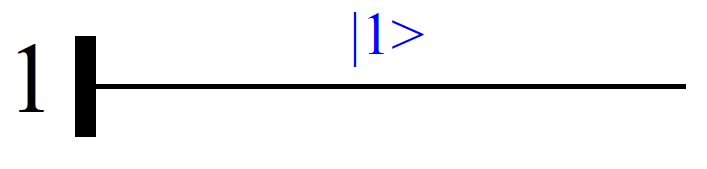
Figure 2: Circuit for hello_world function

Apply Quantum Gates :

From hello_world function, we get a quantum state. Now we will apply a quantum gate on that qubit. At this point, we will take the advantage of Quipper’s higher order functionality that means a function can be passed through another function. We will name our function apply_gate and pass hello_world function as parameter. apply_gate function will use hello_world to convert a classical state into a quantum state and apply a quantum gate on it. The code is given below:

– declare apply_gate function

apply_gate :: (Bool $\rightarrow$ Circ Qubit) $\rightarrow$ Bool $\rightarrow$ Circ Qubit

apply_gate func bool = do

– use func function to get qubit

qbit $\leftarrow$ func bool

– to comment on pdf circuit

comment "before gate"

– apply Hadamard Transfomation

qbit $\leftarrow$ hadamard qbit

– both label and comment

comment_with_label "after gate" (qbit) ("$(|0\rangle-|1\rangle)/2$")

– return result

return qbit

– main function to call the whole program

main = print_simple Preview (apply_gate hello_world True)

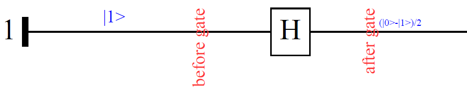
Figure 3: Circuit for apply_gate function

The "type signature" of apply_gate tells that it has two arguments. First one is a function (Bool $\rightarrow$ Circ Qubit) that takes a Bool and returns a Qubit, second one is a Bool data type. This function returns a Qubit. To apply Hadamard Transformation we can use hadamard or gate_H operator (box represents quantum gate in pdf of Quipper). We can also use gate_H_at or hadamard_at, these operators don’t return any value, in that case expression should be like hadamard_at qbit. We may use other quantum gates like qnot, gate_X, gate_S, gate_Z, gate_T, gate_Y etc.

In the main function, we pass the hello_world function and a "True" Bool type data through apply_gate function. hello_world and True values are stored respectively in func and bool variables. Finally this function returns a quantum state after applying hadamard transformation.

Data Structures:

As Quipper’s host language is Haskell, it mainly uses Haskell’s data structures. Haskell provides many data structures like Map, Set etc, but now we would like to focus on the most basic data structures that are list and tuple. let and where clauses are used for local bindings (we will use these in the implementations).

list in Haskell is a linked list, it uses (:) operator to bind an element. (++) operator is used for concatenation. head operator is used to get the first element of a list and tail is used to get the rest. Operator (!!) is used to find the element of an index. [Bool] and [Qubit] are the example of list. lists are homogeneous that means a single list can contain only single type of elements. On the other hand, tuple is a fixed number of single or different type components. tuple is mainly used for returning multiple values of different data types. (Qubit, Bool) and ([Qubit], [Qubit]) are the examples of tuple.

Previously we performed hadamard transformation only on one qubit. To perform hadamard transformations on multiple qubits, we will use list of qubits, [Qubit]. In that case, we will need to modify the type signature of hello_world and apply_gate functions like hello_world :: [Bool] $\rightarrow$ Circ [Qubit] and apply_gate :: ([Bool] $\rightarrow$ Circ [Qubit]) $\rightarrow$ [Bool] $\rightarrow$ Circ [Qubit]. To perform quantum gates on a list, we will use mapUnary operator. Then expression should be like mapUnary hadamard qbit instead of qbit $\leftarrow$ hadamard qbit, in apply_gate function.

In the main function we will use replicate operator and where clause to create n True Bool type data. We will also use print_generic as circuit shape is not fixed here. The main function is:

– main function to call the whole program

main = print_generic Preview (apply_gate hello_world (replicate n True))

where

n = 5

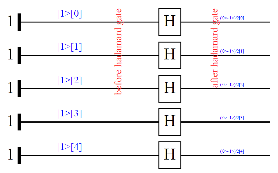
Figure 4: Circuit of applying gates on multiple qubits

Measurement Operation :

Quipper provides measure operator to measure quantum states and cdiscard operator to discard classical data. These two are generic operators that means any data structure can be applied here. measure operator takes Qubit and collapses it to one of the basic states. cdiscard operator takes classical Bits and discards. and notations are used respectively to denote measure and cdiscard operations. We will use these operators in our controlled_gate function that applies a controlled gate operation on two qubits and measures their values. Corresponding code is given below:

– declare controlled_gate function

controlled_gate :: (Bool, Bool) $\rightarrow$ Circ Bit

controlled_gate (cntrl_qbit, trget_qbit) = do

– convert Bool into Qubit

cntrl_qbit $\leftarrow$ qinit cntrl_qbit

trget_qbit $\leftarrow$ qinit trget_qbit

– controlled gate operation

gate_X_at trget_qbit ‘controlled‘ cntrl_qbit

– measure Qubits

(cntrl_qbit, trget_qbit) $\leftarrow$ measure (cntrl_qbit, trget_qbit)

– discard value

cdiscard trget_qbit

– return result

return cntrl_qbit

– main function

main = print_simple Preview (controlled_gate (False,True))

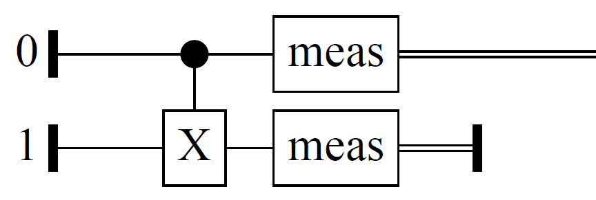
Figure 5: Circuit of measurement example

Here we apply a X gate on trget_qbit with the control of cntrl_qbit. To do that we use ‘controlled‘ operator. We can also use this operator for list data structure. Then the expression will be like ‘controlled‘ list. To specify their controlling states we can write the expression like ‘controlled‘ list .==. [0,1,0] (assume list has three elements).

Quipper gives the opportunity to apply "Unitary Operations" using matrix. We can do the previous example using $4\times 4$ matrix. We will import some additional libraries and write a function operator that have the matrix.

– import Matrix constructors

import Libraries.Synthesis.Matrix

import QuipperLib.Synthesis

import Libraries.Synthesis.Ring

– initialize unitary matrix

operator :: Matrix Four Four DOmega

operator = matrix4x4 ( 1, 0, 0, 0 )

( 0, 1, 0, 0 )

( 0, 0, 0, 1 )

( 0, 0, 1, 0 )

In controlled_gate function, if we change gate_X_at trget_qbit ‘controlled‘ cntrl_qbit expression into exact_synthesis operator [cntrl_qbit, trget_qbit] expression, main function will generate the same previous circuit. More tutorials on Quipper can be found in [11].

4 Implementation of quantum algorithms

Quantum algorithms are interesting because for some cases it gives exponential computational power like factoring integers, finding orders of functions. Instead of being one state at a time, quantum computer gives the opportunity to the states to be in a superposition. To get the superposition, many quantum algorithms initialize $n$ qubits with $|0\rangle$ and apply Hadamard transformation. It maps $n$ qubits to the superpositions of all $2^{n}$ orthogonal states in the $|0\rangle,|1\rangle$ basis with equal weight.

Here we implement five quantum algorithms in Quipper Programming Language. Section 4.1 describes the Deutsch’s algorithm which determines the fairness of a boolean function. Section 4.2 is the Deutsch-Jozsa algorithm which is the generalized version of Deutsch’s algorithm. Section 4.3 is Simon’s periodicity algorithm that finds the hidden pattern of a function. Section 4.4 describes Grover’s search algorithm that can search an element from unordered array in $\sqrt{n}$ time. Finally section 4.5 describes Shor’s factoring algorithm which can factor integers in polynomial time.

4.1 Deutsch algorithm

The Deutsch algorithm, published in 1985 [8], solves a contrived problem to see how quantum computers can be used. This algorithm actually determines if a function is one to one or not. A function is called balanced if $f(0)\neq f(1)$, means one to one. Otherwise a function is called constant if $f(0)=f(1)$. Deutsch’s algorithm solves the following problem (we quote the definition of the problem verbatim from [25]):

Problem 1.

Given a function $f:\{0,1\}\rightarrow\{0,1\}$ as a black box, where one can evaluate an input, but cannot "look inside" and "see" how the function is defined, determine if the function is balanced or constant.

Classical algorithm needs two steps (first step to find $f(0)$’s value and second step to find $f(1)$’s value) to determine and Deutsch algorithm needs one step. This algorithm provides an oracle separation between P and EQP.

First, we will write codes for Deutsch algorithm. Then we will code oracles (black boxes) of balanced and constant functions and finally, test those oracles using the simulator provided by Quipper.

4.1.1 Quantum circuit for Deutsch algorithm

As we have to test an oracle whether it is balanced or constant, at first we will write our own data type named Oracle. Later we will declare our oracles of functions using this data type. Main section of Deutsch algorithm will be in deutsch_circuit function. Finally main function will call deutsch_circuit function with an oracle named empty_oracle. here empty_oracle is a dummy oracle, we will use this to generalize the circuit. Later we will use some working oracles. main function will get a classical data Bit to determine whether given oracle is balanced or constant. The code for deutsch_circuit is:

import Quipper

– declare Oracle data type

data Oracle = Oracle{

– oracle of function $f(x)$

oracle_function :: (Qubit,Qubit) $\rightarrow$ Circ (Qubit,Qubit)

}

– declare deutsch_circuit function

deutsch_circuit :: Oracle $\rightarrow$ Circ Bit

deutsch_circuit oracle = do

– create the ancillae

top_qubit $\leftarrow$ qinit False

bottom_qubit $\leftarrow$ qinit True

label (top_qubit, bottom_qubit) ("$|0\rangle$","$|1\rangle$")

– do the first Hadamards

hadamard_at top_qubit

hadamard_at bottom_qubit

comment "before oracle"

– call the oracle

oracle_function oracle (top_qubit, bottom_qubit)

comment "after oracle"

– do the last Hadamards

hadamard_at top_qubit

– measure qubits

(top_qubit, bottom_qubit) $\leftarrow$ measure (top_qubit, bottom_qubit)

– discard un-necessary output and return the result

cdiscard bottom_qubit

return top_qubit

– main function to call the whole program

main = print_generic Preview (deutsch_circuit empty_oracle)

where

– declare empty_oracle’s data type

empty_oracle :: Oracle

empty_oracle = Oracle {

oracle_function = empty_oracle_function

}

– initialize empty_oracle

empty_oracle_function:: (Qubit,Qubit) $\rightarrow$ Circ (Qubit,Qubit)

empty_oracle_function (one,two) = named_gate "Oracle" (one,two)

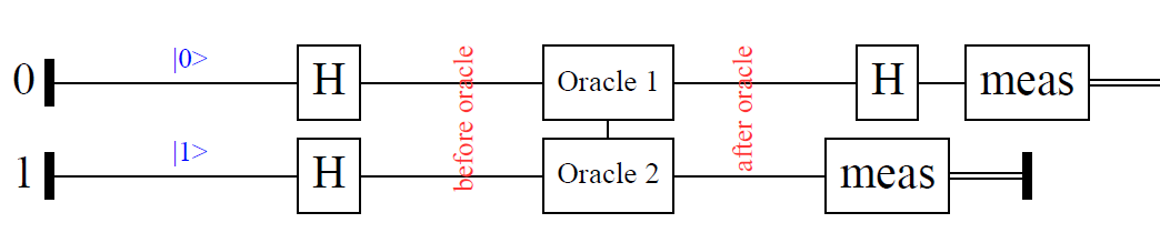
Figure 6: Circuit for Deutsch algorithm [25]

4.1.2 Oracle examples

Balanced Oracle :

We will write code for balanced oracle in balanced_oracle. Here we will perform a controlled not operation. This will be a balanced oracle because here $f(0)\neq f(1)$. Finally main function will pass this oracle to deutsch_circuit function. So the modified section is:

main = print_generic Preview (deutsch_circuit balanced_oracle)

where

– declare balanced_oracle’s data type

balanced_oracle :: Oracle

balanced_oracle = Oracle {

oracle_function = balanced_oracle_function

}

– initialize oracle function $f(x)$

balanced_oracle_function:: (Qubit,Qubit) $\rightarrow$ Circ (Qubit,Qubit)

balanced_oracle_function (x,y) = do

qnot_at y ‘controlled‘ x

return (x,y)

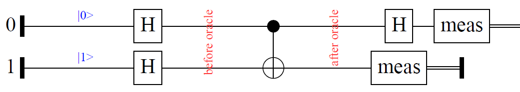
Figure 7: Circuit for balanced oracle

Constant Oracle:

We will write code for constant oracle in constant_oracle. We will remain qubits states same so that this oracle will ensure $f(0)=f(1)$. In main function, we will pass this oracle to deutsch_circuit function. So the modified section is:

main = print_generic Preview (deutsch_circuit constant_oracle)

where

– declare constant_oracle’s data type

constant_oracle :: Oracle

constant_oracle = Oracle {

oracle_function = constant_oracle_function

}

– initialize oracle function $f(x)$

constant_oracle_function:: (Qubit,Qubit) $\rightarrow$ Circ (Qubit,Qubit)

constant_oracle_function (x,y) = do

– Qubits will remain the same

return (x,y)

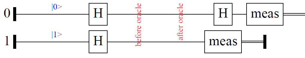
Figure 8: Circuit for constant oracle

4.1.3 Simulation

We can test previous oracles with the simulator included in Quipper. We will remove balanced_oracle, constant_oracle functions from where clause and write those functions independently. We will write two new functions simulate and circuit. In simulate function, we will test the oracle using built-in run_generic function and in circuit function, we will show the simulation results. main function is to start the whole program.

– import modules for simulations

import qualified Data.Map as Map

import QuipperLib.Simulation

import System.Random

– declare simulate function

simulate :: Circ Bit $\rightarrow$ Bool

simulate oracle = (run_generic (mkStdGen 1) (1.0::Double) oracle)

Let’s highlight Quipper’s built-in run_generic function for simulation. It takes three arguments:

1. A source of randomness, something of type StdGen from Haskell’s System.Random library. mkStdGen is a function creating such an object out of an Int. So (mkStdGen 1) does the trick.

2. An instance of real number so that the function run_generic knows what to use as datatype for reals. Here we take Double.

3. The circuit to run.

circuit function will take simulate function and an Oracle . IO() represents this function has an I/O operation. simulate function will return a Bool type data True when oracle is balanced and False when oracle is constant. circuit function will take the result and perform an I/O operation. main function should be modified. When we will run the program in command prompt, we get the simulation results "Given oracle is Balanced" for balanced oracles and "Given oracle is Constant" for constant oracles.

– declare circuit function

circuit :: (Circ Bit $\rightarrow$ Bool) $\rightarrow$ Oracle $\rightarrow$ IO ()

circuit run oracle =

– first deutsch_circuit will apply on oracle

– then run function will evaluate the result

if run (deutsch_circuit oracle)

then putStrLn "Given oracle is Balanced"

else putStrLn "Given oracle is Constant"

– main function

main = do

– test constant_oracle

circuit simulate constant_oracle

– test balanced_oracle

circuit simulate balanced_oracle

Figure 9: Simulation of Deutsch Algorithm

4.2 Deutsch-Jozsa algorithm

The Deutsch-Jozsa algorithm, proposed by David Deutsch and Richard Jozsa in 1992 [9], is the generalized version of Deutsch algorithm, which accepts a string of $n~{}0$’s and $1$’s and outputs a zero or one.

A function is called balanced if exactly half of the input’s outputs are $0$’s and other half of the input’s outputs are $1$’s. And a function is called constant if all the input’s outputs are either $0$’s or $1$’s. Deutsch-Jozsa algorithm solves the following problem (we quote the definition of the problem verbatim from [25]):

Problem 2.

Given a function $f:\{0,1\}^{n}\rightarrow\{0,1\}$ as a black box, where one can evaluate an input, but cannot "look inside" and "see" how the function is defined, determine if the function is balanced or constant.

For classical algorithm, the best case scenario is when first two inputs have different outputs which ensures that given function is balanced. But to ensure a function is constant, it must evaluate the function more than half of the possible inputs. So it requires $\frac{2^{n}}{2}+1=2^{(n-1)}+1$ evaluations. But Deutsch-Jozsa algorithm solves this problem in one evaluation, provides an oracle separation of P and EQP, that’s an exponential speedup.

4.2.1 Circuit of Deutsch-Jozsa algorithm

Unlike Deutsch algorithm, the Deutsch-Jozsa algorithm accepts a string of length $n$. That’s why we will need to augment our previous Oracle data type so that it can deal with the string of qubits. The core section of Deutsch-Jozsa algorithm will be in deutsch_jozsa_circuit function (more or less similar to deutsch_circuit function). In the main function, we will call deutsch_jozsa_circuit with a dummy oracle named empty_oracle. So the code for Deutsch-Jozsa algorithm is:

import Quipper

– declare modified Oracle data type

data Oracle = Oracle {

– declare the length of a string

qubit_num :: Int,

– declare oracle function $f(x)$

function :: ([Qubit], Qubit) $\rightarrow$ Circ ([Qubit], Qubit)

}

– declare deutsch_jozsa_circuit function

deutsch_jozsa_circuit :: Oracle $\rightarrow$ Circ [Bit]

deutsch_jozsa_circuit oracle = do

– initialize string of qubits

top_qubits $\leftarrow$ qinit (replicate (qubit_num oracle) False)

bottom_qubit $\leftarrow$ qinit True

label (top_qubit, bottom_qubit) ("$|0\rangle$","$|1\rangle$")

– do the first hadamard

mapUnary hadamard top_qubits

hadamard_at bottom_qubit

comment "before oracle"

– call oracle

function oracle (top_qubits, bottom_qubit)

comment "after oracle"

– do the last hadamard

mapUnary hadamard top_qubits

– measure qubits

(top_qubits, bottom_qubit) $\leftarrow$ measure (top_qubits, bottom_qubit)

– discard unnecessary output and return result

cdiscard bottom_qubit

return top_qubits

– main function

main = print_generic Preview (deutsch_jozsa_circuit empty_oracle)

where

– declare empty_oracle’s data type

empty_oracle :: Oracle

empty_oracle = Oracle {

qubit_num = 5,

function = empty_oracle_function

}

– initialize empty_oracle’s function $f(x)$

empty_oracle_function:: ([Qubit],Qubit) $\rightarrow$ Circ ([Qubit],Qubit)

empty_oracle_function (ins,out) = named_gate "Oracle" (ins,out)

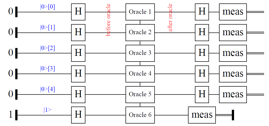
Figure 10: Circuit for Deutsch-Jozsa algorithm [25]

4.2.2 Oracle examples

Constant Oracle:

We will write code for constant oracle in constant_oracle. For all inputs of this function, outputs will be either $0$ or $1$ that means $f(x)=0$ for all $x$ or $f(x)=1$ for all $x$. The code for constant_oracle is given below:

main = print_generic Preview (deutsch_jozsa_circuit constant_oracle)

where

– declare constant_oracle’s data type

constant_oracle :: Oracle

constant_oracle = Oracle {

qubit_num = 2,

function = constant_oracle_function

}

– initialize constant_oracle function $f(x)$

constant_oracle_function:: ([Qubit],Qubit) $\rightarrow$ Circ ([Qubit],Qubit)

constant_oracle_function (ins,out) = do

– Qubits will remain the same

return (ins, out)

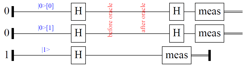
Figure 11: Circuit for constant oracle

Balanced Oracle:

We will write code for balanced oracle in balanced_oracle. Exactly half of the inputs for this function will go for $0$’s and other half will go for $1$’s as output that means $f(x)=0$ for half of $x$ and $f(x)=1$ for other half of $x$.

main = print_generic Preview (deutsch_jozsa_circuit balanced_oracle)

where

– declare balanced_oracle’s data type

balanced_oracle :: Oracle

balanced_oracle = Oracle {

qubit_num = 2,

function = balanced_oracle_function

}

– initialize balanced_oracle function $f(x)$

balanced_oracle_function:: ([Qubit],Qubit) $\rightarrow$ Circ ([Qubit],Qubit)

balanced_oracle_function ([x,y],out) = do

qnot_at out ‘controlled‘ x

qnot_at out ‘controlled‘ y

return ([x,y],out)

balanced_oracle_function _ = error "undefined" – fallback case

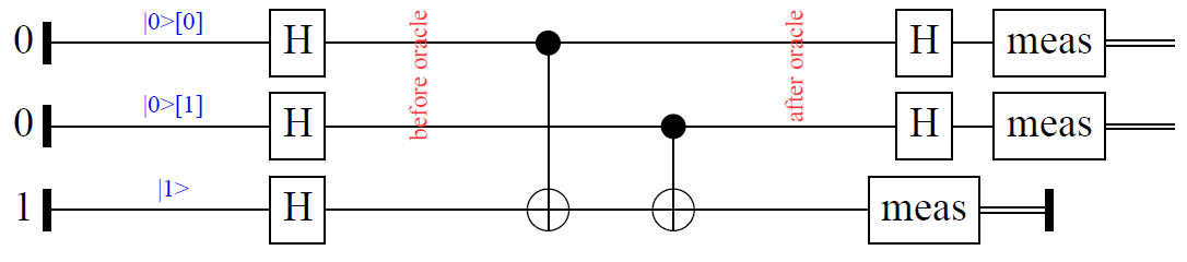
Figure 12: Circuit for balanced oracle

4.2.3 Simulation

Like in the Deutsch algorithm, we will write a new simulate function that simulates oracles classically and a new circuit function to show the simulation results.

import qualified Data.Map as Map

import QuipperLib.Simulation

import System.Random

– simulate function

simulate :: Circ [Bit] $\rightarrow$ Bool

simulate oracle = and (map not (run_generic (mkStdGen 1) (1.0::Float) oracle))

Here simulate function uses map operator to apply not to each elements of the oracle to negate its values. Then and operator is applied to the results and finally returns a Bool. circuit function will use the Bool to print "constant" for constant oracles (when Bool is True) and "balanced" for balanced oracles (when Bool is False). Again, main function will be used to start the whole program.

– circuit function

circuit :: (Circ [Bit] $\rightarrow$ Bool) $\rightarrow$ Oracle $\rightarrow$ IO ()

circuit run oracle =

– first deutsch_jozsa will apply on oracle

– then run function will evaluate the result

if run (deutsch_jozsa_circuit oracle)

then putStrLn "constant"

else putStrLn "balanced"

– main function

main = do

– test constant_oracle

circuit simulate constant_oracle

– test balanced_oracle

circuit simulate balanced_oracle

Figure 13: Simulation of Deutsch-Jozsa algorithm

4.3 Simon’s periodicity algorithm

Simon’s periodicity algorithm is about finding patters in a particular set of functions that’s why it is a promised problem. It solves Simon’s problem which is a computational problem in the model of decision tree complexity or query complexity, conceived by Daniel Simon in 1994 [23]. It was also the inspiration for Shor’s algorithm (we will discuss at section 4.5). Both problems are special cases of the abelian hidden subgroup problem. Simon’s algorithm has both quantum procedures and classical procedures. We will mainly discuss about quantum procedures. Simon’s algorithm solves the following problem (we quote the definition of the problem verbatim from [25]):

Problem 3.

Given a function $f:\{0,1\}^{n}\rightarrow{\{0,1\}}^{n}$ as a black box, promised to have a secret (hidden) binary string s, such that for all strings x, y $\in{\{0,1\}}^{n}$, we have f(x)=f(y) if and only if $\textbf{x = y }\oplus\textbf{ s}$. The goal is to determine s.

In other words, the values of $f$ repeat themselves in some pattern and the pattern is determined by $s$. Function $f$ is one to one when $s=0^{n}$ otherwise $f$ is two to one. If we find two inputs $x_{1},x_{2}$ such that $f(x_{1})=f(x_{2})$, then $x_{1}=x_{2}\oplus s$ and we obtain $s$ by $x_{1}\oplus x_{2}=x_{2}\oplus s\oplus x_{2}=s$

The worst case scenario for classical algorithm to determine a two to one function is, it needs more than half of the inputs evaluations. So it requires $\frac{2^{n}}{2}+1=2^{n-1}+1$ function evaluations. On the contrary, Simon’s algorithm needs $n$ function evaluations. Classical computational model needs exponential time complexity to solve this problem while quantum computational model solves it in bounded quantum polynomial time.

4.3.1 Circuit for Simon’s algorithm

The core section of Simon’s algorithm will be written in simon_circuit function. The quantum part of Simon’s algorithm is basically performing this function several times. We will write function steps for running simon_circuit $n-1$ times. This function will return a Maybe data type that mean’s it may return ([Bit], [Bit]) or may return Nothing (readers may think like null value). We will get only the binary string which satisfies $\langle y,s\rangle=0$ . When $\langle y,s\rangle=1$, destructive interference occurs which cancels each other and we get nothing. Classical part of Simon’s algorithm will take that results and solves "linear equations" to find hidden pattern $s$. This can be done by Gaussian elimination, which takes $\Omega{(n^{3})}$ steps.

import Quipper

– declare oracle data type

data Oracle = Oracle {

qubit_num :: Int,

function :: ([Qubit], [Qubit]) $\rightarrow$ Circ ([Qubit], [Qubit])

}

– declare simon_circuit function

simon_circuit :: Oracle $\rightarrow$ Circ ([Bit], [Bit])

simon_circuit oracle = do

–create the ancillaes

top_qubits $\leftarrow$ qinit (replicate (qubit_num oracle) False)

bottom_qubits $\leftarrow$ qinit (replicate (qubit_num oracle) True)

label (top_qubits, bottom_qubits) ("top |0>", "bottom |1>")

– apply first hadamard gate

mapUnary hadamard top_qubits

mapUnary hadamard bottom_qubits

– call the oracle

(function oracle) (top_qubits, bottom_qubits)

– apply hadamard gate again

mapUnary hadamard top_qubits

– measure qubits

(top_qubits, bottom_qubits) $\leftarrow$ measure(top_qubits, bottom_qubits)

– return the result

return (top_qubits,bottom_qubits)

– declare steps function

steps :: (Oracle $\rightarrow$ Circ ([Bit], [Bit])) $\rightarrow$ Oracle $\rightarrow$ Circ (Maybe ([Bit], [Bit]))

steps simon_algorithm oracle = do

comment " Simon’s algorithm"

– set value for n

let n = toEnum (qubit_num oracle) :: Int

– call simon_circuit n-1 times

for 1 (n-1) 1 $ \i $\rightarrow$ do

comment "start"

– call simon_circuit function

ret $\leftarrow$ simon_algorithm oracle

– return the result

return ret

comment "finish"

endfor

return Nothing

– declare main function

main = print_generic Preview (steps simon_circuit empty_oracle)

where

– declare empty_oracle’s data type

empty_oracle :: Oracle

empty_oracle = Oracle {

– set the length of qubit string

qubit_num = 4,

function = empty_oracle_function

}

– initialize empty_oracle’s function

empty_oracle_function:: ([Qubit],[Qubit]) $\rightarrow$ Circ ([Qubit],[Qubit])

empty_oracle_function (ins,out) = named_gate "Oracle" (ins,out)

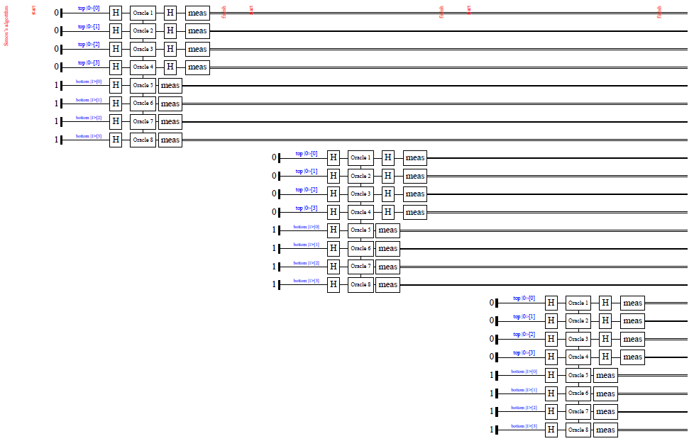
Figure 14: Quantum subroutine for Simon’s algorithm [5]

4.3.2 Oracle example

We will write code for an oracle when qubit_num = 2. So, the inputs are 00, 01, 10 and 11. Let’s consider the period, s = 11. So, we can define the function as follows:

$f(00)=01,f(01)=10,f(10)=f(01\oplus 11)=10$ and $f(11)=f(00\oplus 11)=01$

The Unitary Transformation is: $|x\rangle|y\rangle\rightarrow|x\rangle|y\oplus f(x)\rangle$. We will code the Unitary matrix in sample_oracle function. The truth table and the code for sample_oracle function is given below:

Table 1: Truth table of unitary matrix

$x$	$y$	$f(x)$	$y\oplus f(x)$	$x$	$y$	$f(x)$	$y\oplus f(x)$	$x$	$y$	$f(x)$	$y\oplus f(x)$	$x$	$y$	$f(x)$	$y\oplus f(x)$
00	00	01	01	01	00	10	10	10	00	10	10	11	00	01	01
00	01	01	00	01	01	10	11	10	01	10	11	11	01	01	00
00	10	01	11	01	10	10	00	10	10	10	00	11	10	01	11
00	11	01	10	01	11	10	01	10	11	10	01	11	11	01	10

– declare sample_oracle’s data type

sample_oracle :: Oracle

sample_oracle = Oracle{

qubit_num = 2,

function = sample_function

}

– initialize sample_oracle’s function

sample_function :: ([Qubit],[Qubit]) $\rightarrow$ Circ ([Qubit],[Qubit])

sample_function (controlled_qubit, target_qubit) = do

let element = controlled_qubit ++ target_qubit

– call the unitary matrix

exact_synthesis operator element

return (controlled_qubit, target_qubit)

– initialize 16 by 16 unitary matrix

operator :: Matrix Sixteen Sixteen DOmega

operator = matrix16x16 ( 0, 1, 0, 0, 0, 0, 0, 0, 0, 0, 0, 0, 0, 0, 0, 0 )

( 1, 0, 0, 0, 0, 0, 0, 0, 0, 0, 0, 0, 0, 0, 0, 0 )

( 0, 0, 0, 1, 0, 0, 0, 0, 0, 0, 0, 0, 0, 0, 0, 0 )

( 0, 0, 1, 0, 0, 0, 0, 0, 0, 0, 0, 0, 0, 0, 0, 0 )

( 0, 0, 0, 0, 0, 0, 1, 0, 0, 0, 0, 0, 0, 0, 0, 0 )

( 0, 0, 0, 0, 0, 0, 0, 1, 0, 0, 0, 0, 0, 0, 0, 0 )

( 0, 0, 0, 0, 1, 0, 0, 0, 0, 0, 0, 0, 0, 0, 0, 0 )

( 0, 0, 0, 0, 0, 1, 0, 0, 0, 0, 0, 0, 0, 0, 0, 0 )

( 0, 0, 0, 0, 0, 0, 0, 0, 0, 0, 1, 0, 0, 0, 0, 0 )

( 0, 0, 0, 0, 0, 0, 0, 0, 0, 0, 0, 1, 0, 0, 0, 0 )

( 0, 0, 0, 0, 0, 0, 0, 0, 1, 0, 0, 0, 0, 0, 0, 0 )

( 0, 0, 0, 0, 0, 0, 0, 0, 0, 1, 0, 0, 0, 0, 0, 0 )

( 0, 0, 0, 0, 0, 0, 0, 0, 0, 0, 0, 0, 0, 1, 0, 0 )

( 0, 0, 0, 0, 0, 0, 0, 0, 0, 0, 0, 0, 1, 0, 0, 0 )

( 0, 0, 0, 0, 0, 0, 0, 0, 0, 0, 0, 0, 0, 0, 0, 1 )

( 0, 0, 0, 0, 0, 0, 0, 0, 0, 0, 0, 0, 0, 0, 1, 0 )

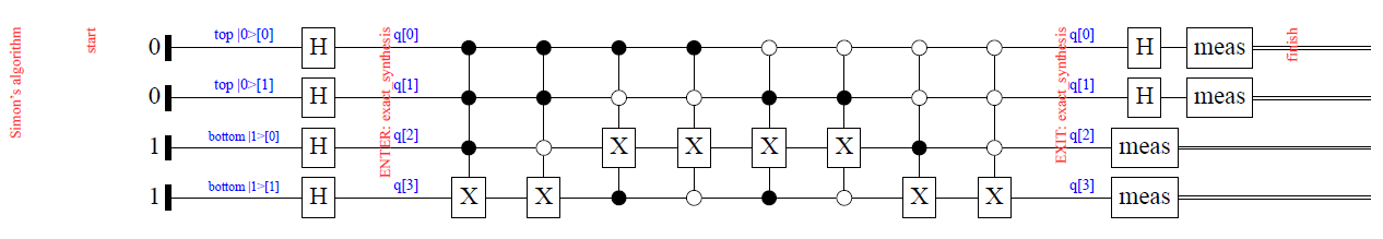
Figure 15: Circuit for sample_oracle function

16 by 16 matrix constructor :

In previous function, we have implemented $16\times 16$ unitary matrix. As Quipper 0.5 version doesn’t include $16\times 16$ matrix constructor, we coded this in Libraries.Synthesis.Matrix module. This module provides fixed but arbitrary sized vectors and matrices. Its dimensions are determined by type level programming. We create a type level representation for number $16$. Ten and Succ are the type representations of number $10$ and successor operation, previously declared in this module. $16\times 16$ matrix constructor is matrix16x16 which takes rows as arguments. Respective codes are given below:

– The natural number 16 as a type

type Sixteen = Succ (Succ (Succ (Succ (Succ (Succ Ten)))))

– A convenience constructor for $16\times 16$ matrices

matrix16x16 ::(a, a, a, a, a, a, a, a, a, a, a, a, a, a, a, a)$\rightarrow$

(a, a, a, a, a, a, a, a, a, a, a, a, a, a, a, a)$\rightarrow$

(a, a, a, a, a, a, a, a, a, a, a, a, a, a, a, a)$\rightarrow$

(a, a, a, a, a, a, a, a, a, a, a, a, a, a, a, a)$\rightarrow$

(a, a, a, a, a, a, a, a, a, a, a, a, a, a, a, a)$\rightarrow$

(a, a, a, a, a, a, a, a, a, a, a, a, a, a, a, a)$\rightarrow$

(a, a, a, a, a, a, a, a, a, a, a, a, a, a, a, a)$\rightarrow$

(a, a, a, a, a, a, a, a, a, a, a, a, a, a, a, a)$\rightarrow$

(a, a, a, a, a, a, a, a, a, a, a, a, a, a, a, a)$\rightarrow$

(a, a, a, a, a, a, a, a, a, a, a, a, a, a, a, a)$\rightarrow$

(a, a, a, a, a, a, a, a, a, a, a, a, a, a, a, a)$\rightarrow$

(a, a, a, a, a, a, a, a, a, a, a, a, a, a, a, a)$\rightarrow$

(a, a, a, a, a, a, a, a, a, a, a, a, a, a, a, a)$\rightarrow$

(a, a, a, a, a, a, a, a, a, a, a, a, a, a, a, a)$\rightarrow$

(a, a, a, a, a, a, a, a, a, a, a, a, a, a, a, a)$\rightarrow$

(a, a, a, a, a, a, a, a, a, a, a, a, a, a, a, a)$\rightarrow$Matrix Sixteen Sixteen a

matrix16x16   (a0, a1, a2, a3, a4, a5, a6, a7, a8, a9, a10, a11, a12, a13, a14, a15)

(b0, b1, b2, b3, b4, b5, b6, b7, b8, b9, b10, b11, b12, b13, b14, b15)

(c0, c1, c2, c3, c4, c5, c6, c7, c8, c9, c10, c11, c12, c13, c14, c15)

(d0, d1, d2, d3, d4, d5, d6, d7, d8, d9, d10, d11, d12, d13, d14, d15)

(e0, e1, e2, e3, e4, e5, e6, e7, e8, e9, e10, e11, e12, e13, e14, e15)

(f0, f1, f2, f3, f4, f5, f6, f7, f8, f9, f10, f11, f12, f13, f14, f15)

(g0, g1, g2, g3, g4, g5, g6, g7, g8, g9, g10, g11, g12, g13, g14, g15)

(h0, h1, h2, h3, h4, h5, h6, h7, h8, h9, h10, h11, h12, h13, h14, h15)

(i0, i1, i2, i3, i4, i5, i6, i7, i8, i9, i10, i11, i12, i13, i14, i15)

(j0, j1, j2, j3, j4, j5, j6, j7, j8, j9, j10, j11, j12, j13, j14, j15)

(k0, k1, k2, k3, k4, k5, k6, k7, k8, k9, k10, k11, k12, k13, k14, k15)

(l0, l1, l2, l3, l4, l5, l6, l7, l8, l9, l10, l11, l12, l13, l14, l15)

(m0, m1, m2, m3, m4, m5, m6, m7, m8, m9, m10, m11, m12, m13, m14, m15)

(n0, n1, n2, n3, n4, n5, n6, n7, n8, n9, n10, n11, n12, n13, n14, n15)

(o0, o1, o2, o3, o4, o5, o6, o7, o8, o9, o10, o11, o12, o13, o14, o15)

(p0, p1, p2, p3, p4, p5, p6, p7, p8, p9, p10, p11, p12, p13, p14, p15) =

matrix        [[a0, b0, c0, d0, e0, f0, g0, h0, i0, j0, k0, l0, m0, n0, o0, p0],

[a1, b1, c1, d1, e1, f1, g1, h1, i1, j1, k1, l1, m1, n1, o1, p1],

[a2, b2, c2, d2, e2, f2, g2, h2, i2, j2, k2, l2, m2, n2, o2, p2],

[a3, b3, c3, d3, e3, f3, g3, h3, i3, j3, k3, l3, m3, n3, o3, p3],

[a4, b4, c4, d4, e4, f4, g4, h4, i4, j4, k4, l4, m4, n4, o4, p4],

[a5, b5, c5, d5, e5, f5, g5, h5, i5, j5, k5, l5, m5, n5, o5, p5],

[a6, b6, c6, d6, e6, f6, g6, h6, i6, j6, k6, l6, m6, n6, o6, p6],

[a7, b7, c7, d7, e7, f7, g7, h7, i7, j7, k7, l7, m7, n7, o7, p7],

[a8, b8, c8, d8, e8, f8, g8, h8, i8, j8, k8, l8, m8, n8, o8, p8],

[a9, b9, c9, d9, e9, f9, g9, h9, i9, j9, k9, l9, m9, n9, o9, p9],

[a10,b10,c10,d10,e10,f10,g10,h10,i10,j10,k10,l10,m10,n10,o10,p10],

[a11,b11,c11,d11,e11,f11,g11,h11,i11,j11,k11,l11,m11,n11,o11,p11],

[a12,b12,c12,d12,e12,f12,g12,h12,i12,j12,k12,l12,m12,n12,o12,p12],

[a13,b13,c13,d13,e13,f13,g13,h13,i13,j13,k13,l13,m13,n13,o13,p13],

[a14,b14,c14,d14,e14,f14,g14,h14,i14,j14,k14,l14,m14,n14,o14,p14],

[a15,b15,c15,d15,e15,f15,g15,h15,i15,j15,k15,l15,m15,n15,o15,p15]]

For 8 by 8 matrix:

We also write code for $8\times 8$ matrix constructor named matrix8x8 in Libraries.Synthesis.Matrix module. It also takes rows as argument.

– define $8\times 8$ matrix constructor

matrix8x8::(a, a, a, a, a, a, a, a) $\rightarrow$ (a, a, a, a, a, a, a, a) $\rightarrow$

(a, a, a, a, a, a, a, a) $\rightarrow$ (a, a, a, a, a, a, a, a) $\rightarrow$

(a, a, a, a, a, a, a, a) $\rightarrow$ (a, a, a, a, a, a, a, a) $\rightarrow$

(a, a, a, a, a, a, a, a) $\rightarrow$ (a, a, a, a, a, a, a, a) $\rightarrow$ Matrix Eight Eight a

matrix8x8  (a0, a1, a2, a3, a4, a5, a6, a7) (b0, b1, b2, b3, b4, b5, b6, b7)

(c0, c1, c2, c3, c4, c5, c6, c7) (d0, d1, d2, d3, d4, d5, d6, d7)

(e0, e1, e2, e3, e4, e5, e6, e7) (f0, f1, f2, f3, f4, f5, f6, f7)

(g0, g1, g2, g3, g4, g5, g6, g7) (h0, h1, h2, h3, h4, h5, h6, h7) =

matrix    [[a0, b0, c0, d0, e0, f0, g0, h0], [a1, b1, c1, d1, e1, f1, g1, h1],

[a2, b2, c2, d2, e2, f2, g2, h2], [a3, b3, c3, d3, e3, f3, g3, h3],

[a4, b4, c4, d4, e4, f4, g4, h4], [a5, b5, c5, d5, e5, f5, g5, h5],

[a6, b6, c6, d6, e6, f6, g6, h6], [a7, b7, c7, d7, e7, f7, g7, h7]]

4.4 Grover’s search algorithm

Grover’s search algorithm is a quantum algorithm for searching an unsorted database with $N$ entries in O($\sqrt{N}$) time and using O($\log N$) storage space, invented by Lov Grover in 1996 [13]. Grover’s search algorithm solves the following problem (we quote the definition of the problem verbatim from [25]):

Problem 4.

Given a function $f:\{0,1\}^{n}\rightarrow\{0,1\}$ as a black box, exists exactly one binary string $x_{0}$ such that $f(x)=1$ if $x=x_{0}$ and $f(x)=0$ if $x\neq x_{0}$. The goal is to find $x_{0}$.

Classically to solve this problem, it needs $\frac{N}{2}$ time on average and $N$ time in worst case scenario. Unlike previous quantum algorithms, Grover’s search algorithm provides a quadratic speedup. Some of the classical algorithms have linear time complexity and quantum algorithm solves the same problem in complexity class BQP.

It uses two tricks to increase the probability of desired binary string $x_{0}$.

1. Phase inversion: is used to change the phase of the desired state.

2. Inversion about the average: is used to boost the separation of the phases.

These operations should not be done more than $\sqrt{N}$ times. Otherwise, for over computation the probability of desired binary string may decrease.

4.4.1 Circuit for Grover’s search algorithm

The core section of Grover’s search algorithm is in grover_search_circuit function. This function calls phase_inversion and inversion_about_mean functions for $\sqrt{2^{n}}$ times. These functions act as their names suggest. phase_inversion function will take an oracle, a qubit string and apply that oracle function on that qubit string. inversion_about_mean function will separate target qubit and controlled qubit from qubit string and apply $2|\psi\rangle\langle\psi|-I$, the conditional phase shift operation [19]. Finally main function will call grover_search_circuit with a dummy oracle named empty_oracle. Respective codes are given below:

import Quipper

– declare Oracle data type

data Oracle = Oracle {

qubit_num :: Int,

function :: ([Qubit], Qubit) $\rightarrow$ Circ ([Qubit], Qubit)

}

– declare phase_inversion function

phase_inversion::(([Qubit],Qubit)$\rightarrow$Circ([Qubit],Qubit))$\rightarrow$([Qubit],Qubit)$\rightarrow$ Circ([Qubit],Qubit)

phase_inversion oracle (top_qubits, bottom_qubit) = do

comment "start phase inversion"

– call oracle

oracle (top_qubits, bottom_qubit)

comment "end phase inversion"

return (top_qubits, bottom_qubit)

– declare inversion_about_mean function

inversion_about_mean :: ([Qubit], Qubit) $\rightarrow$ Circ ([Qubit], Qubit)

inversion_about_mean (top_qubits, bottom_qubit) = do

comment "start inversion about mean"

– apply X gate at top qubit

mapUnary gate_X top_qubits

– separate target and control qubits

let pos = (length top_qubits) - 1

let target_qubit = top_qubits !! pos

let controlled_qubit = take pos top_qubits

– apply hadamard at target_qubit

hadamard_at target_qubit

– apply qnot gate at target qubit

qnot_at target_qubit ‘controlled‘ controlled_qubit

– apply hadamard again at top

hadamard_at target_qubit

– apply X gate at bottom

mapUnary gate_X top_qubits

comment "end inversion about mean"

return (top_qubits, bottom_qubit)

– declare grover_search_circuit function

grover_search_circuit :: Oracle $\rightarrow$ Circ ([Bit])

grover_search_circuit oracle = do

comment "Grover Search algorithm"

– set the value of n

let n = toEnum (qubit_num oracle) :: Float

– set the index number to iterate $\sqrt{2^{n}}$ times

let index = (floor (sqrt (2**n))) :: Int

– create the ancillaes

top $\leftarrow$ qinit (replicate (qubit_num oracle) False)

bottom $\leftarrow$ qinit True

label (top, bottom) ("|0>","|1>")

– apply hadamard gate at string

mapUnary hadamard top

hadamard_at bottom

– start to iterate

for 1 (index) 1 $ \i $\rightarrow$ do

comment "start grover iteration"

– call phase inversion

(top, bottom) $\leftarrow$ phase_inversion (function oracle) (top, bottom)

– call inversion about mean

(top, bottom) $\leftarrow$ inversion_about_mean (top, bottom)

comment "after grover iteration"

endfor

– measure qubit string and return result

hadamard_at bottom

(top, bottom) $\leftarrow$ measure (top, bottom)

cdiscard bottom

return (top)

– main function

main = print_generic Preview (grover_search_circuit empty_oracle)

where

– declare empty_oracle’s data type

empty_oracle :: Oracle

empty_oracle = Oracle {

– set the length of qubit string

qubit_num = 4,

function = empty_oracle_function

}

– initialize empty_oracle’s function $f(x)$

empty_oracle_function:: ([Qubit],Qubit) $\rightarrow$ Circ ([Qubit],Qubit)

empty_oracle_function (ins,out) = named_gate "Oracle" (ins,out)

Figure 16: Circuit for Grover’s search algorithm

4.4.2 Oracle examples

Single Grover iteration :

We will code for single Grover iteration in oracle_two. This oracle will find the search element $x_{0}=2$ in search space size $N=4$ [19]. So oracle’s reaction will be $f(x)=1$ when $x=x_{0}=2$ and $f(x)=0$ when $x\neq 2$. oracle_two function is:

– declare oracle_two data type

oracle_two :: Oracle

oracle_two = Oracle {

qubit_num = 2,

function = oracle_two_function

}

– initialize oracle_two function $f(x)$

oracle_two_function :: ([Qubit],Qubit) $\rightarrow$ Circ ([Qubit],Qubit)

oracle_two_function (controlled_qubit, target_qubit) = do

qnot_at target_qubit ‘controlled‘ controlled_qubit .==. [1,0]

return (controlled_qubit, target_qubit)

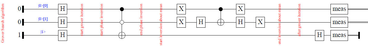
Figure 17: Circuit for Grover’s single iteration $(x_{0}=2)$ [15] [19]

Multiple Grover iteration :

oracle_five function needs multiple Grover’s iteration to fine search element $x_{0}=5$ in search space size $N=8$. This function will behave like $f(x)=1$ when $x=x_{0}=5$ and $f(x)=0$ when $x\neq 5$. oracle_five function is:

– declare oracle_five’s data type

oracle_five :: Oracle

oracle_five = Oracle {

qubit_num = 3,

function = oracle_five_function

}

– initialize oracle_five’s function

oracle_five_function :: ([Qubit],Qubit) $\rightarrow$ Circ ([Qubit],Qubit)

oracle_five_function (controlled_qubit, target_qubit) = do

qnot_at target_qubit ‘controlled‘ controlled_qubit .==. [1,0,1]

return (controlled_qubit, target_qubit)

Figure 18: Circuit for Grover’s multiple iteration $(x_{0}=5)$ [15]

4.5 Shor’s factoring algorithm

Shor’s algorithm, the most celebrated quantum algorithm is formulated by Peter Shor in 1994 [22] for integer factorization. Like Simon’s periodicity algorithm, Shor’ algorithm uses phase estimation procedure to factor integers in polynomial time. This factoring problem turns out to be equivalent to the order finding problem discussed in Simon’s algorithm. Shor’s algorithm uses two basic steps to reduce factoring procedure to order finding procedure. These two steps are embodied in the following theorems (we quote these theorems verbatim from [19]):

Theorem 1.

Suppose N is a n bit composite number, and a is a non-trivial solution to the equation $\textbf{a}^{2}$ = 1(mod N) in the range 1$\leq$ a $\leq$ N, that is, neither a = 1(mod N) nor a = N$-1$ = $-1$(mod N). Then at least one of gcd($\textbf{a}-1$, N) and gcd($\textbf{a}+1$, N) is a non-trivial factor of N.

Theorem 2.

Suppose N = $p_{1}^{\alpha_{1}}..p_{m}^{\alpha_{m}}$ is the prime factorization of an odd composite positive integer. Let a be an integer chosen uniformly at random, subject to the requirements that $1\leq\textbf{a}\leq N-1$ and a is co-prime to N. Let r be the order of a modulo N. Then

p(r is even and $\textbf{a}^{r/2}\neq-1(mod~{}N))\geq 1-\frac{1}{2^{m}}$

All these theorems can be implemented in classical part, but quantum part needs to find the periods of the functions that hold big integers. We can formally state Shor’s algorithm like below [25]:

Step 1:

First check if $N$ is a prime or a power of prime. Polynomial algorithm can be used to determine it. If yes then declare it and exit. Otherwise go to the next step.

Step 2:

Choose a random integer a such that $1<\textbf{a}<N$ and then determine $gcd(\textbf{a},N)$ using Euclid’s algorithm. If the GCD is not 1, then return it and exit.

Step 3:

Quantum subroutine for finding the period $r$ of a function.

Step 4:

If $r$ is odd or if $\textbf{a}^{r}\equiv-1~{}mod~{}N$, then chosen a is not appropriate for further calculations. Go back to step 2 and choose another a.

Step 5:

Calculate $gcd((\textbf{a}^{\frac{r}{2}}+1),N)$ and $gcd((\textbf{a}^{\frac{r}{2}}-1),N)$ using Euclid’s algorithm and return at least one of the nontrivial solutions.

Shor’s algorithm needs $O(n^{2}~{}log~{}n~{}log~{}log~{}n)$ number of steps, where $n$ is the number of bit to represent $N$. On the contrary, best known classical algorithm requires $O(\exp^{cn^{\frac{1}{3}}log^{\frac{2}{3}}n})$ where $c$ is some constant. Classical algorithms work in sub-exponential time and Shor’s algorithm solves it in the complexity class BQP. Here quantum algorithm gives an exponential speedup. Here we will mainly discuss the quantum subroutine of Shor’s algorithm.

4.5.1 Circuit for Shor’s algorithm

The main section of Shor’s algorithm is written in shor_circuit function. In this function, oracle $f_{(a,N)}(x)$ will be applied to find it’s period $r$. Then $QFT^{\dagger}$ will be applied to modify the period $r$ into $\frac{2^{top\_num}}{r}$ and to eliminate the offset. Quipper provides QuipperLib.QFT module to perform Quantum Fourier Transformation. We will use qft_big_endian function of this module to apply $QFT^{\dagger}$ on top_qubit. Finally main function will pass a dummy oracle named empty_oracle to shor_circuit function and start the whole program.

import Quipper

import QuipperLib.QFT

– define oracle data type

data Oracle = Oracle {

top_num :: Int,

bottom_num :: Int,

function :: ([Qubit], [Qubit]) $\rightarrow$ Circ ([Qubit], [Qubit])

}

– declare shor_circuit function

shor_circuit :: Oracle $\rightarrow$ Circ [Bit]

shor_circuit oracle = do

comment "Shor algorithm"

– create the ancillaes

top_qubit $\leftarrow$ qinit (replicate (top_num oracle) False)

bottom_qubit $\leftarrow$ qinit (replicate (bottom_num oracle) False)

label (top_qubit, bottom_qubit) ("top_qubit", "bottom_qubit")

– apply hadamard at top qubits

mapUnary hadamard top_qubit

comment "applying oracle"

– call the oracle

function oracle (top_qubit, bottom_qubit)

comment "after oracle"

– measure bottom qubits and discard

bottom_qubit $\leftarrow$ measure bottom_qubit

cdiscard bottom_qubit

– apply $QFT^{\dagger}$

top_qubit $\leftarrow$ qft_big_endian top_qubit

– measure top qubits and return results

top_qubit $\leftarrow$ measure top_qubit

return top_qubit

– main function

main = print_generic Preview (shor_circuit empty_oracle)

where

– declare empty_oracle’s data type

empty_oracle :: Oracle

empty_oracle = Oracle {

top_num = 6,

bottom_num = 3,

function = empty_function

}

– initialize empty_oracle’s function $f(x)$

empty_function :: ([Qubit], [Qubit]) $\rightarrow$ Circ ([Qubit], [Qubit])

empty_function (top, bottom) = named_gate "Oracle" (top,bottom)

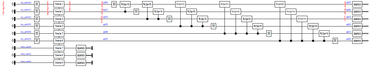
Figure 19: Quantum subroutine for Shor’s algorithm[2]

4.5.2 Oracle examples

We will write an oracle $f_{(a,N)}(x)$ where $a=7$ and $N=15$ [2]. Corresponding oracle mod15_base7_oracle is given below:

– declare mod15_base7_oracle data type

mod15_base7_oracle :: Oracle

mod15_base7_oracle = Oracle{

top_num = 3,

bottom_num = 4,

function = mod15_base7_function

}

– initialize mod15_base7_oracle’s function $f(x)$

mod15_base7_function :: ([Qubit], [Qubit]) $\rightarrow$ Circ ([Qubit], [Qubit])

mod15_base7_function (top_qubit, bottom_qubit) = do

let x1 = top_qubit !! 1

let x2 = top_qubit !! 2

let y0 = bottom_qubit !! 0

let y1 = bottom_qubit !! 1

let y2 = bottom_qubit !! 2

let y3 = bottom_qubit !! 3

qnot_at y1 ‘controlled‘ x2

qnot_at y2 ‘controlled‘ x2

qnot_at y2 ‘controlled‘ y0

qnot_at y0 ‘controlled‘ [x1,y2]

qnot_at y2 ‘controlled‘ y0

qnot_at y1 ‘controlled‘ y3

qnot_at y3 ‘controlled‘ [x1,y1]

qnot_at y1 ‘controlled‘ y3

return (top_qubit, bottom_qubit)

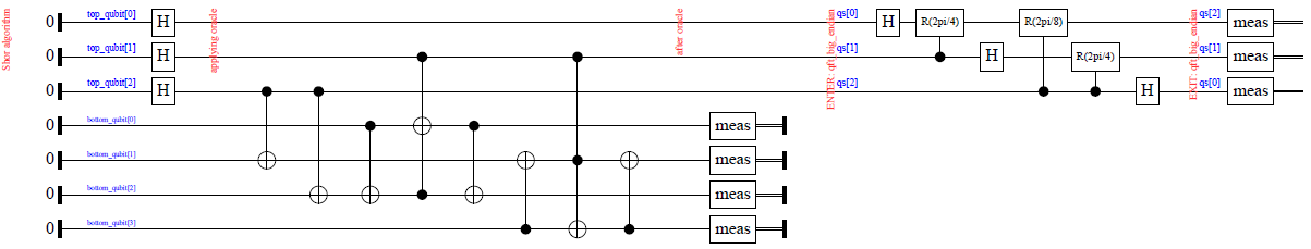
Figure 20: Circuit for an oracle of $f_{(a,N)},a=7,N=15$ [2]

We will write another oracle $f_{(a,N)}(x)$ where $a=20$ and $N=21$. We will optimize quantum circuits for modular multiplication [16]. Code for mod21_base20_oracle is given below:

– declare mod21_base20_oracle data type

mod21_base20_oracle :: Oracle

mod21_base20_oracle = Oracle{

top_num = 3,

bottom_num = 5,

function = mod21_base20_function

}

– initialize mod21_base20_oracle function

mod21_base20_function :: ([Qubit], [Qubit]) $\rightarrow$ Circ ([Qubit], [Qubit])

mod21_base20_function (top_qubit, bottom_qubit) = do

– separate control qubit

let cntrl_qbit = head top_qubit

– separate $y_{0},y_{2}$ and $y_{4}$

let y0 = head bottom_qubit

let y2 = head (drop 2 bottom_qubit)

let y4 = head (drop 4 bottom_qubit)

– apply quantum gates

qnot_at y4 ‘controlled‘ cntrl_qbit

qnot_at y2 ‘controlled‘ cntrl_qbit

qnot_at y0 ‘controlled‘ cntrl_qbit .==. 0

return (top_qubit, bottom_qubit)

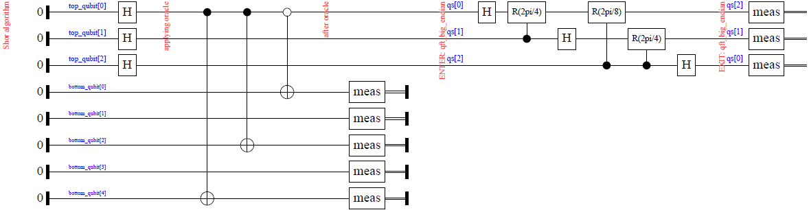
Figure 21: Circuit for an oracle of $f_{(a,N)},a=20,N=21$ [16]

5 Conclusion

This report mainly targets the readers who are interested to study functional quantum programming language. We briefly discussed about some other classes of quantum programming languages. We have introduced readers to Quipper and implemented five quantum algorithms using it. It demonstrates the capability of the language and the work overhead for quantum programmers. Starting from a "hello world" program we demonstrated up to Shor’s factoring algorithm in a pedagogically suitable sequence in order to ensure a smooth learning carve. We have also given examples of high dimensional oracles (black boxes or functions) for specific algorithms and test some of them using Quipper simulator.

6 Acknowledgement

SS thanks the Quipper authors Benoît Valiron and Peter Selinger for their continuous help in understanding the language throughout the project. He also likes to thank Professor Md. Shahidur Rahman for giving permission to pursue this project through an experimental distance learning setup. OS thanks Professor Samuel J. Lomonaco Jr. for his comments.

References

- [1] Intelligence advanced research projects activity. https://www.fbo.gov/notices/637e87ac1274d030ce2ab69339ccf93c. [Accessed May 2, 2014].
- [2] Nature: International weekly journal of science. http://www.nature.com/nature/journal/v414/n6866/fig_tab/414883a_F1.html%. [Accessed May 27, 2014].
- [3] The quipper language. http://www.mathstat.dal.ca/~selinger/quipper/. [Accessed April 27, 2014].
- [4] Wikipedia: Quantum programming. http://en.wikipedia.org/wiki/Quantum_programming. [Accessed May 2, 2014].
- [5] Wikipedia: Simon’s problem. http://en.wikipedia.org/wiki/Simon’s_problem. [Accessed: April 27, 2014].
- [6] Thorsten Altenkirch and Jonathan Grattage. A functional quantum programming language. In Logic in Computer Science, 2005. LICS 2005. Proceedings. 20th Annual IEEE Symposium on, pages 249–258. IEEE, 2005.
- [7] Stefano Bettelli, Tommaso Calarco, and Luciano Serafini. Toward an architecture for quantum programming. The European Physical Journal D-Atomic, Molecular, Optical and Plasma Physics, 25(2):181–200, 2003.
- [8] David Deutsch. Quantum theory, the church-turing principle and the universal quantum computer. Proceedings of the Royal Society of London. A. Mathematical and Physical Sciences, 400(1818):97–117, 1985.
- [9] David Deutsch and Richard Jozsa. Rapid solution of problems by quantum computation. Proceedings of the Royal Society of London. Series A: Mathematical and Physical Sciences, 439(1907):553–558, 1992.
- [10] Simon J Gay. Quantum programming languages: Survey and bibliography. Mathematical Structures in Computer Science, 16(4):581–600, 2006.
- [11] Alexander S Green, Peter LeFanu Lumsdaine, Neil J Ross, Peter Selinger, and Benoît Valiron. An introduction to quantum programming in quipper. In Reversible Computation, pages 110–124. Springer, 2013.
- [12] Alexander S Green, Peter LeFanu Lumsdaine, Neil J Ross, Peter Selinger, and Benoît Valiron. Quipper: A scalable quantum programming language. In Proceedings of the 34th ACM SIGPLAN conference on Programming language design and implementation, pages 333–342. ACM, 2013.
- [13] Lov K Grover. A fast quantum mechanical algorithm for database search. In Proceedings of the twenty-eighth annual ACM symposium on Theory of computing, pages 212–219. ACM, 1996.
- [14] Emmanuel Knill. Conventions for quantum pseudocode. Technical report, Citeseer, 1996.
- [15] Carlile Lavor, LRU Manssur, and Renato Portugal. Grover’s algorithm: quantum database search. arXiv preprint quant-ph/0301079, 2003.
- [16] Igor L Markov and Mehdi Saeedi. Constant-optimized quantum circuits for modular multiplication and exponentiation. Quantum Information & Computation, 12(5-6):361–394, 2012.
- [17] Wolfgang Mauerer. Semantics and simulation of communication in quantum programming. arXiv preprint quant-ph/0511145, 2005.
- [18] Jaroslaw Adam Miszczak. Models of quantum computation and quantum programming languages. arXiv preprint arXiv:1012.6035, 2010.
- [19] Michael A Nielsen and Isaac L Chuang. Quantum computation and quantum information. Cambridge university press, 2010.
- [20] Bernhard Ömer. A procedural formalism for quantum computing. 1998.
- [21] Peter Selinger. Towards a quantum programming language. Mathematical Structures in Computer Science, 14(4):527–586, 2004.
- [22] Peter W Shor. Algorithms for quantum computation: discrete logarithms and factoring. In Foundations of Computer Science, 1994 Proceedings., 35th Annual Symposium on, pages 124–134. IEEE, 1994.
- [23] D.R. Simon. On the power of quantum computation. In Foundations of Computer Science, 1994 Proceedings., 35th Annual Symposium on, pages 116–123, Nov 1994.
- [24] André van Tonder. A lambda calculus for quantum computation. SIAM Journal on Computing, 33(5):1109–1135, 2004.
- [25] Noson S Yanofsky and Mirco A Mannucci. Quantum computing for computer scientists, volume 20. Cambridge University Press Cambridge, 2008.
- [26] Paolo Zuliani. Quantum programming. PhD thesis, University of Oxford, 2001.