Mid-Infrared Selected Quasars I: Virial Black Hole Mass and Eddington Ratios

Abstract

We provide a catalog of 391 mid-infrared-selected (MIR, 24 $\mu$m) broad-emission-line (BEL, type 1) quasars in the 22 deg² SWIRE Lockman Hole field. This quasar sample is selected in the MIR from Spitzer MIPS with $S_{\rm 24}>400\mu$Jy, jointly with an optical magnitude limit of r (AB) $<$ 22.5 for broad line identification. The catalog is based on MMT and SDSS spectroscopy to select BEL quasars, extends the SDSS coverage to fainter magnitudes and lower redshifts, and recovers a more complete quasar population. The MIR-selected quasar sample peaks at $z\sim$1.4, and recovers a significant and constant (20%) fraction of extended objects with SDSS photometry across magnitudes, which was not included in the SDSS quasar survey dominated by point sources. This sample also recovers a significant population of $z<3$ quasars at $i>19.1$. We then investigate the continuum luminosity and line profiles of these MIR quasars, and estimate their virial black hole masses and the Eddington ratios. The SMBH mass shows evidence of downsizing, though the Eddington ratios remain constant at $1<z<4$. Compared to point sources in the same redshift range, extended sources at $z<1$ show systematically lower Eddington ratios. The catalog and spectra are publicly available online.

1 INTRODUCTION

The apparent connection between supermassive black holes (SMBHs) and their host galaxies has been explained by a variety of theories. In the merger driven model, the collision of dust-rich galaxies drives gas inflows, fueling both starbursts and buried quasars until feedback disperses the gas and dust, allowing the quasar to be briefly visible as a bright optical source (e.g. Sanders et al., 1988; Hopkins et al., 2006). Instead of physical coupling between the BH and host galaxy, the central-limit-theorem can be used to explain the linear SMBH mass and bulge mass correlation by the hierarchical assembly of BH and stellar mass (Peng, 2007; Jahnke & Macciò, 2011). Alternatively, the cold flow model (e.g. Dekel et al., 2009; Bournaud et al., 2011; Di Matteo et al., 2012) introduces inflowing cosmological cold gas streams rather than collisions to fuel the star formation and quasar, and better explains the clumpy disks observed for high-$z$ galaxies. Observationally, a SMBH-host connection is supported by the discovery of correlations of the SMBH mass with bulge luminosity, mass, and velocity dispersion, especially with bulges and ellipticals (e.g. Kormendy & Richstone, 1995; Ferrarese & Merritt, 2000; Kormendy & Ho, 2013). However, despite tremendous progress on the demographic studies of SMBHs, whether or how the SMBH regulates the formation and evolution of their hosts via the possible ‘feedback’ process is still under debate. One sign of such feedback may be the ongoing star formation observed for host galaxies of active galactic nuclei (AGNs) and quasars, and vice versa, starbursts are found to host buried AGNs (Kauffmann et al., 2003; Shi et al., 2009; Dai et al., 2012). Based on the similar star formation rate (SFR) observed for galaxies with and without an active galactic nucleus (AGN), recent studies suggest that the SMBH-host correlation results from the gas availability, instead of major interaction between the SMBH growth and host star formation (e.g. Goulding et al., 2014; Lilly et al., 2013). In this paper, we present a mid-infrared (MIR) selection to effectively select quasar candidates with dusty nuclear material in a disk/wind or torus geometry (e.g. Elvis, 2000; Antonucci, 1993, ‘torus’ hereafter). This selection is relatively unaffected by obscuration.

In the high redshift ($z>0.5$) universe, it is hard to observe both broad-line (type 1) quasars and their host galaxies simultaneously. The quasar glare usually outshines the host galaxy at optical wavelengths, and the host has a small angular size. In large optical surveys, the focus has been on broad-emission-line (BEL) quasars (e.g. Richards et al., 2006a; Shen et al., 2011, S11), or ‘blue’ quasars, which are biased towards optically-unobscured (Type 1) objects with limited information about the host galaxy. Studies on the cosmic history of quasars show an evolution over redshifts, with a quasar peak appearing at $z\sim$ 1.5 (e.g. Hasinger et al., 2005; Silverman et al., 2008). At longer infrared (IR) wavelengths, where thermal emission from dust is dominant, quasars have characteristic power-law shaped MIR SEDs, and are selected by different color wedges in the Spitzer IRAC (Fazio et al., 2004) and Wide-field Infrared Survey Explorer (Wright et al., 2010, WISE) bands (Lacy et al., 2004; Sajina et al., 2005; Stern et al., 2005, 2012; Donley et al., 2012).

Recent surveys in the IR have detected optically obscured (type 2), dust-reddened quasars (e.g. Richards et al., 2003, 2009; Polletta et al., 2006; Glikman et al., 2012; Lacy et al., 2013). These quasars are marked by having reddened UV-optical SEDs resulting from dust absorption. At different redshift and luminosity ranges, quasars are reported to have an obscuration fraction from 20% to over 50% (Lacy et al., 2002; Glikman et al., 2004, 2007; Urrutia et al., 2009; Juneau et al., 2013; Lacy et al., 2013). In the merger-driven model, these quasars are in an early transitional phase, and are in the process of expelling their dusty environment before becoming ‘normal’ blue quasars (type 1). This IR-luminous phase also evolves with time, and was more common at high $z$ (e.g. Caputi et al., 2007; Serjeant et al., 2010). Optical studies of quasar and host systems are challenged by the high contrast between the bright point-source quasar and starlight. Infrared-selected quasars are good candidates to study the SMBH-host connection, as they are not biased against dusty hosts.

In this paper, we present a catalog of 391 MIR-selected BEL objects in the $\sim$22 deg² Lockman Hole - Spitzer Wide-area InfraRed Extragalactic Survey (LHS) Field (SWIRE, Lonsdale et al., 2003). As will be pointed out in §2.6, since all of the objects have BEL features, and the majority also qualify the classical Seyfert / quasar luminosity separation ($M_{\rm B}<-23$), hereafter we will simply refer to these BEL objects as quasars. Combining the mid-IR (MIR) 24 $\mu$m flux-limit and optical identification has been demonstrated to be an effective way of selecting quasars (with a 13% detection rate in Papovich et al. (2006)). This MIR selection was designed to be biased towards dusty systems, where ample hot dust exists in the nuclear region with higher likelihood of tracing remnant or ongoing star formation (cool dust). The spectroscopic sample used in this work comprises new observations taken with the Hectospec at the MMT of the wide-angle SWIRE field and of a smaller MIPS GTO field, and spectra obtained by the Sloan Digital Sky Survey (SDSS) within the Lockman Hole footprint. We hope that this sample will provide a new test bed to study the SMBH self-regulation or AGN feedback when the system has not relaxed to equilibrium, if such effects do exist. In §2 we review the sample selection and introduce the spectroscopic data and the MIR additions to the SDSS quasar catalog; followed by the spectral measurements in §3; in §4 and §5, we describe the virial black hole mass and bolometric luminosity estimates; we then follow with the spectral catalog (§6), discussion (§7) and the summary (§8). Throughout the paper, we assume a concordance cosmology with $H_{0}$=70 km$/$s Mpc^-1, $\Omega_{\rm M}$=0.3, and $\Omega_{\Lambda}$=0.7. All magnitudes are in AB system except where otherwise noted.

2 THE SAMPLE

2.1 MIR MIPS 24 $\mu$m Selection

The combined MIR 24 $\mu$m and optical selection for this survey was designed to detect objects with luminous torus / nucleus and not biased against dusty hosts. The MIR selection allows detection of hot dust (a few hundred K) at the redshifts z$\sim$1.5; while optical follow-up spectroscopically identified the BEL objects , confirming their unobscured (type 1) quasar nature. This MIR selection also allows far-infrared (FIR) cross-match to look for cool dust for SMBH-host studies, as demonstrated in Dai et al. (2012).

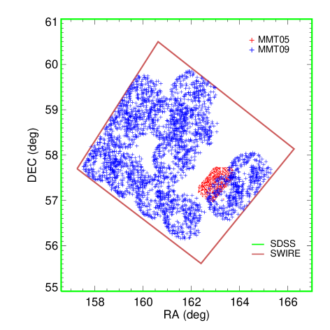
Figure 1: Spectroscopic targets and survey coverage in the Lockman Hole-SWIRE (LHS) field: Green square, SDSS photometry, covering the whole field; Brown square, SWIRE; Red pluses, MMT-Hectospec (2005); Blue pluses, MMT-Hectospec (2009). The hole at the center of each MMT configuration is due to the spacing limitation of the 300 fibers in the Hectospec instrument.

We select Spitzer MIPS (Rieke et al., 2004) 24 $\mu$m sources from the SWIRE survey in the $\sim$ 22 deg² Lockman Hole - SWIRE (LHS) field centered at RA$=$10:46:48, DEC$=$57:54:00 (Lonsdale et al., 2003). The SDSS imaging also covers the LHS region to $r=22.2$ at 95 % detection repeatability, but can go as deep as $r=23$. All magnitudes are taken from the SDSS photoObj catalog in DR7, already corrected for Galactic extinction according to Schlegel, Finkbeiner, & Davis (1998). They are the SDSS approximate AB system (Oke & Gunn, 1983; Fukugita et al., 1996; Smith et al., 2002). SDSS has astrometric uncertainties $<0.1\arcsec$ on average . In Fig. 1 we show the SWIRE and SDSS coverages in the LHS field.

We first apply a 24 $\mu$m flux limit of 400 $\mu$Jy ($\sim$ 8 $\sigma$), which yields a sample of 23, 402 objects. The completeness at 400 $\mu$Jy for SWIRE-MIPS catalog is $\sim$ 90% (Shupe et al., 2008). The confusion limit due to extragalactic sources for MIPS 24 $\mu$m band is 56 $\mu$Jy (Dole et al., 2004), so source confusion is not an issue in this sample. The errors in position for these sources are between 0.2$\arcsec$–0.4$\arcsec$, and the effective beam size (FWHM) of MIPS at 24 $\mu$m is $\sim 6\arcsec$ .

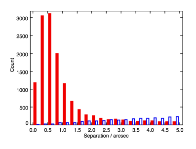
Figure 2: Histogram of the offset between SWIRE and SDSS positions (red). In blue is the same histogram for mismatches after a random position offset ($<$ 10 $\arcsec$ radius). The random association rate within 5 $\arcsec$ is $\sim$18%, but declines to $\sim$6% within 2.5 $\arcsec$. A matching radius of 2.5 $\arcsec$ was used to maximize the matching counts while minimizing the random associations.

We then match the 24 $\mu$m flux limited sources to the SDSS DR7 catalog. We determine an association radius of 2.5 $\arcsec$ to maximize the matching number counts while at the same time minimizing the cases of random association (Fig. 2). We first match the SWIRE and the SDSS r band catalogs. Then we offset the SWIRE position by a random number within 10 $\arcsec$ radius, and match them to the SDSS r band catalog. The association radius is determined by comparing the random association rate at different radii. The random association rate within 5 $\arcsec$ is $\sim$18% (2,467 out of 14,069 matches), but declines to $\sim$6% within 2.5 $\arcsec$. Beyond 2.5 $\arcsec$ radius there are $>50\%$ random associations. The estimated total number of false associations within 2.5 $\arcsec$ is 868 (6%). Adopting the association radius of 2.5 $\arcsec$ we find 14,069 matches. Of these 87$\%$ (12,255) 24 $\mu$m sources also satisfy $r<$ 22.5. This r limit allows follow-up optical spectroscopic observations with the MMT.

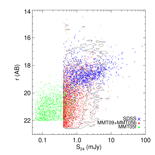
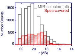
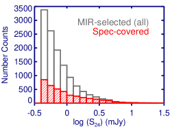
Figure 3: (Top): Spectroscopic coverage in the $S_{\rm 24}-r$ band space for MIR-selected targets: Blue crosses, 854 SDSS DR7 targets; Red, 2,485 MMT09 plus 273 MMT05b targets; Green, 902 MMT05f targets. The contours in the background are the 12,255 MIR-selected targets that satisfy the $S_{\rm 24}>400\mu$Jy (& $r<$ 22.5) limits. (Bottom): The r band magnitude and 24 $\mu$m flux distribution for all MIR-selected targets (black), and the spectroscopic covered objects (Spec-covered, red).

The optical spectroscopic survey consists of four parts (Fig. 3, Table. 1): (1) SDSS DR7; (2) MMT 2009 survey (MMT09); and (3) MMT 2005 bright targets (MMT05b). These three subsamples include the MIR-selected targets as described above. A fourth subsample comes from MMT 2005 observations for MIPS deep targets (§2.4): (4) MMT 2005 faint targets (MMT05f) ($60\,\mu{\rm Jy}\leq S_{\rm 24}<400\,\mu{\rm Jy}$), kept only for comparison purpose. Table 2 summarizes the MMT covered observations.

2.2 SDSS spectroscopy

In order to minimize the need for new spectroscopy, we downloaded and analyzed the existing SDSS spectroscopy of LHS MIPS 24$\mu$m targets directly from the SDSS DR7 SkyServer. The SDSS spectra have a resolving power of R $\sim$1800–2200, with a wavelength coverage of 3800–9200 $\AA$. In this study, we use the ‘1d’ calibrated spectra from the DR7 Data Archive Server, stored in logarithmic pixel scale of 10^-4. The redshifts given in SDSS DR7 SpecObj catalog were determined by the $spectro1d$ package (Stoughton et al., 2002). We made a SQL search (with a 5 degree radius, $r<$ 22.5) in the SDSS DR7 SpecObj catalog and found 2,978 objects. Spectra for all SDSS objects with redshifts in the LHS field were downloaded, irrespective of their SDSS classification. We matched these sources with the SWIRE MIPS 24 $\mu$m catalog, and excluded 2,019 SDSS targets not detected by SWIRE, and 38 SDSS targets with $S_{24}<$400 $\mu$Jy. Within the remaining 921 qualified spectra, we only retain, for BEL identification, the 854 objects (93 %) with a redshift confidence $\geq$ 0.9.

2.3 MMT 2009 Spectroscopy

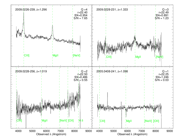
Figure 4: Examples of spectra with different redshift quality flags from Q $=$ 4 (probability $>95\%$ of being correct) to Q $=$1 (no features recognized), following the same procedure as in the DEEP2 survey (Willmer et al., 2006; Newman et al., 2013). Q values are listed in the top right corner; also shown in the top right corner are the SDSS r band magnitude (AB), the MIPS 24 $\mu$m flux in mJy, and the median S/N per pixel in the plotted region (Note this is different from the median S/N of the emission line region, which is usually of a higher value). Typical quasar lines are marked in green. The redshifts given for the Q $=$1 and Q $=$ 2 examples are generated from the code or after visual check, and are not reliable values. Only spectra with Q $\geq$ 3 are kept in this work (See also § 2.5).

Hectospec is a 300 fiber spectrometer with a 1^∘ diameter field of view (FOV) mounted on the MMT (Fabricant et al., 2005; Mink et al., 2007). The combination of a wide field with a large aperture makes Hectospec well-suited to cover extended areas such as the LHS. Hectospec covers a wavelength range of 3650-9200 ${\AA}$ with a 6 ${\AA}$ resolution (1.2 ${\AA}$ pixel^-1, R$=$600–1500). The primary spectroscopic data specific to this study were taken in 2009 (MMT09, PI: Huang) over 11 dark photometric nights with good seeing ($<$ 2 ″) with 12 FOVs. The MMT data cover a total area of $\sim$ 12 deg² (50% of LHS field). An ongoing MMT project (PI: Dai) is complementing the 2009 observations by targeting unobserved areas within the LHS. But the new project adopts a different selection that emphasizes Herschel (Pilbratt et al., 2010) targets, to favor objects with cool dust ($<60K$) that traces the host star formation. These data will be published in a forthcoming paper (Dai et al., in preparation). In Fig. 1 the spectroscopic targets in the 12 fields observed in 2009 are marked as blue pluses. At the center of each MMT FOV, an area with fewer targets can be noticed. This is due to the spacing limitations of Hectospec, whose 300 fibers cannot be crossed or placed less than 50 $\arcsec$ from one another. The $\sim$ 3000 spectroscopic targets were selected from the 11, 401 MIPS and r-band flux limited catalog from §2.1 (after excluding the 854 SDSS objects from §2.2). Brighter 24 $\mu$m sources were given higher priority (See Fig. 3), and fibers were configured to cover as much of the LHS field as possible. Hectospec gives a clear BEL detection (median S/N per pixel $>$ 5 ) for a $r=22.4$ quasar in a 1.5 hour exposure (e.g. Fig. 4, LHS-2009.0226-239). Hence 1.5 hour exposures were used as the standard. Spectra for 2913 objects were recorded in 2009. The optical spectroscopic completeness in the 12 MMT09 Fields is 33% for $S_{\rm 24}>$ 400 $\mu$Jy objects, with an average overlap of 0.08 deg² between different configurations. After taking into account the objects missing due to fiber placement limitations, the completeness of MMT09 sample drops to $\sim$30%, and will be used in the following discussions ($\S~{}\ref{sec:completeness}.$)

2.4 MMT 2005 MIPS-deep Spectroscopy

This spectroscopic sample is extended to include 273 MMT spectra from an earlier 2005 deep survey (MMT05) across eight, highly overlapping FOVs in the LHS. The 2005 data cover a much smaller ($\sim$ 0.5 deg²) region (PI: Papovich). The MMT 2005 survey applied a deeper 24 $\mu$m flux limit of $S_{\rm 24}>$ 60 $\mu$Jy, near to the MIPS confusion limit (Rieke et al., 2004). Only r $<22$ targets were selected in the 2005 observations. MMT05 recorded 1,481 spectra. Of these, 273 objects also satisfy the bright MMT09 limit ($S_{\rm 24}>$ 400 $\mu$Jy) and are included in this sample. We call this the MMT05b (bright) sample. The remaining 1,208 objects with fainter flux (60 $<S_{\rm 24}<$ 400 $\mu$Jy) were also kept for comparison purposes. This sample is designated MMT05f (faint).

The highly overlapped MMT05 FOVs lead to an optical spectroscopy completeness of 66% for 24 $\mu$m bright targets ($S_{\rm 24}>$ 400 $\mu$Jy) in the 0.5 deg² area. This higher completeness comes at the cost of lower efficiency, with an average overlap of 0.94 deg², and a drop from 242 targets per FOV in MMT09 to 185 targets per FOV in MMT05 observations, which encouraged the adoption of the MMT09 strategy.

2.5 Spectral Data Reduction

The SDSS spectra and redshifts are used directly from the DR7 SpecObj catalog without further reduction. The MMT Hectospec data (MMT09, MMT05b and MMT05f) were reduced using the HSRED pipeline (Cool et al., 2008, http://mmto.org/ rcool/hsred/index.html), which is based on the SDSS pipeline. HSRED extracts one dimensional (1d) spectra, subtracts the sky and then flux-calibrates the spectra. The flux-calibration is done using spectra of 6-10 stars selected to have SDSS colors of F stars that are observed simultaneously with the main galaxy and quasar sample. The flux calibration correction is obtained combining the extinction-corrected SDSS photometry of these stars with Kurucz (1993) model fits (Cool et al., 2008). These stellar spectra are also used to remove the telluric lines. The spectral range covered by Hectospec allows detecting one or more typical emission lines present in the spectra of quasars and galaxies (CIV, MgII, H$\beta$, [O_III], H$\alpha$) for galaxies to $z\sim\,1$, and quasars to $z\sim$4.5. The redshifts measured by HSRED also use code adapted from SDSS and use the same templates as SDSS. All spectra were visually inspected for validation as described below.

A redshift quality flag is assigned to each spectrum, following the same procedure used for the DEEP2 survey (Willmer et al., 2006; Newman et al., 2013), where redshift qualities range from Q $=$ 4 (probability P $>95\%$ of being correct), 3 (90$\%<$ P $<95\%$), 2 (P $<90\%$) and 1 (no features recognized). Q $=$ 2 spectra are assigned to objects for which only a single feature is detected, but cannot be identified without ambiguity. The Q $=$ 3 spectra have more than one spectral feature identified, but tend to have low S/N; typical confidence levels for these objects is $\sim$ 90% for the DEEP2 galaxies. Finally, Q $=$ 4 objects have 2 or more spectral features with reasonable to high S/N. The confidence level of these redshifts is typically $>$ 95%. Because of the larger spectral range covered by HECTOSPEC (3800–9500 Å) relative to DEEP2 (5000–9500Å), we expect that the quoted confidence levels are the conservative limits for our spectra.

Fig. 4 shows examples of objects in each redshift quality category. In this study, as for the 854 SDSS spectra, only spectra of Q = 3 and 4 were used. This yields a total of 2,485 MMT09 spectra ($\sim$90% of all the recorded spectra); and 1,175 MMT05 spectra ($\sim$80%). All of the 273 MMT05b subsample satisfy the redshift quality filter.

Table 1: Optical spectroscopic sample summary.

	Source	rAB	S${}_{\rm 24}(\mu$Jy)	Nspec	Nquasar	Covered deg2	Detection rate
(1)	SDSS	$<$ 22.5	$>$400	854*	138*	22	16.2%
(2)	MMT09	$<$ 22.5	$>$400	2485	226	11	9.1 %
(3)	MMT05b	$<$ 22	$>$400	273	27	0.5	9.9%
	Total	$<$ 22.5	$>$400	3612	391	22	10.8%
(4)	MMT05f	$<$ 22	$60<S_{\rm 24}<400$	902	17	0.5	1.9%

*: In the full $\sim$ 22 deg² LHS field. The numbers of spectra and quasars in the $\sim$ 12 deg² MMT-covered regions are 622 and 96, respectively.

Table 2: Observation log for MMT spectroscopic survey.

Instrument	Telescope	RA	Dec	Exposure	Observation Date
		(J2000)	(J2000)	hours
Hectospec	MMT Observatory	$+10:39:48.3$	$+59:16:56$	1.5	2009.0319
Hectospec	MMT Observatory	$+10:48:48.9$	$+58:31:58$	1.5	2009.0318
Hectospec	MMT Observatory	$+10:33:26.2$	$+57:55:05$	1.5	2009.0317
Hectospec	MMT Observatory	$+10:45:21.6$	$+57:53:55$	1.5	2009.0301
Hectospec	MMT Observatory	$+10:37:35.1$	$+57:32:53$	1.2	2009.0228
Hectospec	MMT Observatory	$+10:39:48.3$	$+59:16:56$	1.5	2009.0227
Hectospec	MMT Observatory	$+10:42:20.4$	$+57:05:15$	1.5	2009.0226
Hectospec	MMT Observatory	$+10:37:12.5$	$+58:38:24$	1.5	2009.0223
Hectospec	MMT Observatory	$+10:54:13.1$	$+57:03:57$	1.5	2009.0222
Hectospec	MMT Observatory	$+10:57:45.5$	$+57:34:04$	1.5	2009.0222
Hectospec	MMT Observatory	$+10:44:31.2$	$+58:46:14$	1.5	2009.0220
Hectospec	MMT Observatory	$+10:48:29.3$	$+59:22:27$	1.5	2009.0131
Hectospec	MMT Observatory	$+10:52:31.3$	$+57:24:15$	1.3	2005.0410
Hectospec	MMT Observatory	$+10:51:02.9$	$+57:22:17$	0.6	2005.0409
Hectospec	MMT Observatory	$+10:51:46.1$	$+57:26:32$	0.3	2005.0408
Hectospec	MMT Observatory	$+10:51:02.9$	$+57:22:17$	1.7	2005.0405
Hectospec	MMT Observatory	$+10:52:09.7$	$+57:27:49$	1.0	2005.0310
Hectospec	MMT Observatory	$+10:51:42.2$	$+57:28:01$	1.0	2005.0308
Hectospec	MMT Observatory	$+10:51:42.2$	$+57:28:01$	1.0	2005.0304
Hectospec	MMT Observatory	$+10:52:03.8$	$+57:26:22$	1.0	2005.0308
Hectospec	MMT Observatory	$+10:52:18.8$	$+57:21:53$	1.0	2005.0308

To summarize, we have a total of 3612 spectra of MIR-selected objects with r $<$ 22.5 observed by MMT-Hectospec or chosen from the SDSS SpecObj catalog with a redshift confidence of $>$ 90% (Table 1).

2.6 Broad Line Object Identification

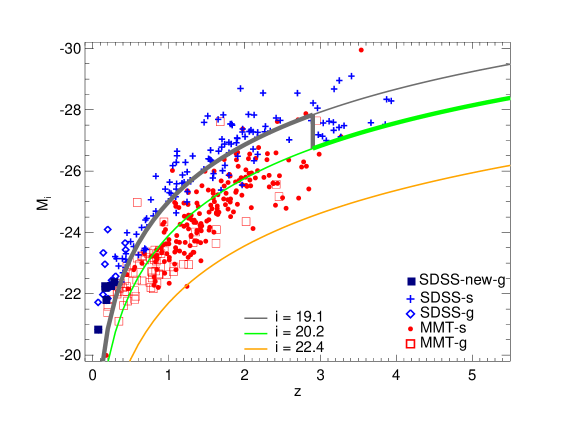
Figure 5: Distribution of MIR-selected quasars in the luminosity-redshift plane. Luminosity is indicated by i band absolute magnitude, $M_{i}$, calculated from the SDSS photometric magnitude. In blue are the SDSS-identified quasars, with blue pluses for point sources and blue diamonds for extended sources; and the red are the MMT-identified quasars, with red dots for point sources and red squares for extended sources. Whether an object is extended (galaxy-like, ‘g’) or a point source (star-like, ‘s’) is defined by the extendedness of the SDSS photometry, see § 2.7.1. The solid navy blue squares mark the 6 quasars newly identified with SDSS spectra that were not included the SDSS DR7 quasar catalog. The curves shows the two magnitude ranges of SDSS selections at $i=19.1$ (grey) and $i=20.2$ (green), and thick curves are the limiting $z$ dependent magnitudes SDSS used for the sample of spectroscopic targets (See § 2.7.1). The orange curve shows the equivalent i band magnitude of the MMT-Hectospec limit ($r=22.4$). A total of 93 new quasars have been identified by MMT (red dots and squares) at $i<20.2$, of which 80 fall between $19.1<i<20.2$ at $z<$ 3, a region SDSS did not cover in the uniform color selection (See also § 2.7). The number densities of $z<3$ quasars is $\sim$ 10 deg^-2 at $i<19.1$, slightly higher than the $\sim$9 deg^-2 at $19.1<i<20.2$.

The 3612 reduced 1d SDSS and Hectospec spectra were first fitted using our IDL program adopted from the S11 procedure. This program fits a polynomial continuum ($S_{\rm continuum}=A_{\rm\lambda}\times(\frac{\lambda}{\lambda_{0}})^{\alpha_{\rm\lambda}}$) and a Gaussian around the redshifted CIV, MgII, and H$\beta$ regions based on the HSRED or SpecObj redshifts (See also §3). Objects are kept as quasar candidates if they have at least one BEL (FWHM $>1000\,\hbox{km s${}^{-1}$}$, Schneider et al. (2007)) in the secure spectral ranges with limited atmospheric extinction and instrument errors: 3850–8400 ${\AA}$ (Fabricant et al., 2008) for MMT targets, and 3850–9000 ${\AA}$ (Stoughton et al., 2002) for SDSS targets. Outside of these ranges the spectra start to be bounded by sky-subtraction errors and therefore not reliable. The MMT range is from Fabricant et al. (2008), chosen to be most consistent ($<5\%$) with SDSS, after comparing the optical spectra taken from SDSS and MMT of the same targets. The IDL program identifies 236 MMT09, 28 MMT05b, and 132 SDSS BEL objects, all of which have an emission line equivalent width (EW) greater than 6. Given our flux limit ($r<22.5$), the majority of the BEL quasars (83% with $Mi<-23$) also satisfy the $M_{\rm B}<-23$, the quasar definition in Schmidt & Green (1983) (Fig. 5). Since the SDSS quasar definition is also based on the BEL features (Schneider et al. (2007)) in the following text we will simply refer to these BEL objects as quasars.

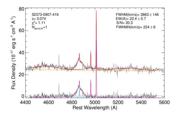
Figure 6: One example of the 6 newly identified SDSS quasar zoomed in at the H$\beta$ emission line region ([4400, 5600] Å). The two sets of plots show in the top the original spectrum (black), the estimated continuum (orange), the scaled Fe template (dark blue) and the final fitted composite spectrum (red). The lower plot shows the continuum- and Fe-template-subtracted spectrum (black), in addition to the variance spectrum (grey), the narrow-line emission component (cyan) and the wide-line component (green). The latter is mostly subsumed by the composite narrow+wide emission line spectrum shown in magenta. The top left corner shows the ID, redshift, fitting $\chi^{2}$ and number of Gaussian component used, and top right is the fitting results (FWHM, EW, signal-to-noise, and the FWHM of the narrow line) in the emission line region.

As a check, we visually examined all 3,612 spectra from both the MMT and SDSS surveys. This process removes 22 MMT09, 1 MMT05b, and 5 SDSS objects that were erroneously identified as quasar due to bad fits. This process also adds 12 MMT09 and 11 SDSS objects, but no MMT05b objects were missed due to a poor fit by the IDL program. Of the 11 SDSS objects, 6 were not included in the SDSS DR7 quasar catalog. All of the 6 new objects are confirmed as quasars with a broad H$\beta$  emission line (Fig. 6 shows one example). We will explore the possible reasons why they were missed in the SDSS DR7 catalog in § 2.7.2. Special objects with interesting features – broad absorption Line (BAL) and narrow absorption line (NAL) quasars — are also flagged (See Section. 7).

Combining the IDL fit and eye check, we identify 226 quasars from the MMT09, 27 from the MMT05b, and 138 from the SDSS DR7 SpecObj catalogs. This adds up to a total of 391 MIR-selected quasars in the LHS field. For comparison, we also scanned the 902 fainter ($S_{\rm 24\,\mu m}<400\mu$Jy) objects from MMT05f survey and identified 17 BEL objects (one was added after eye check). Table 1 summarizes the quasar numbers in each subsample. The fraction of MIR quasars in the MMT09 subsample is 9.1%, and 9.9% in the MMT05b subsample, yielding an average detection rate of 9.2%. After including the SDSS quasars selected through color-color selection, the total detection rate for this MIR quasar sample in LHS field is 10.8%. If only considering the MMT and SDSS overlapping area, the quasar detection rate is an almost identical 10.9%. These detection rates are marginally lower than the $13\pm 3$% reported in Papovich et al. (2006), where a higher 24 $\mu$m flux limit ($S_{\rm 24\,\mu m}>1$ mJy) was applied.

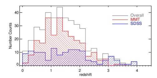
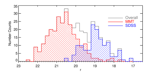
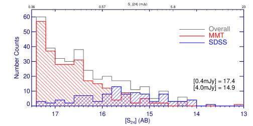
Figure 7: (top) The redshift distribution for the full MIR-selected quasars catalog (grey), the 253 MMT subsample (red), and the 138 SDSS subsample (blue). Middle and bottom panels show the same color coded distribution of SDSS r band magnitude and the 24 $\mu$m flux (converted to AB magnitude for presentation purpose, flux conversion examples are given in the bottom right).

To study the overall properties of the MIR-selected quasars, we plot the redshift ($z$, top), r band magnitude ($r$, middle), and 24 $\mu$m flux ([$S_{24}$], bottom) distributions (Fig. 7). The sample has a redshift range of $0.07<z<3.93$, with a median redshift of 1.3. A K-S test shows significant difference (p $\ll 0.1$) between the SDSS and MMT subsamples in all three parameters ($z,\,S_{24}$,  and $r$). The SDSS quasars have two $z$ peaks at 1$<z<$2 and at $z\sim 3.2$, with an overall median $z=1.5$. The reason for the double peaks is because of the two main color selection criteria ($ugri\ \&\ griz$) applied in SDSS for low-$z$ ($z<2.9$) and high-$z$ ($z>2.9$) quasars (§2.7.1). The MMT, on the other hand, has a roughly Gaussian redshift distribution with a peak at $z\sim$1.3. The MIR-selected quasars are clearly not homogeneously distributed across redshifts. The SDSS subsample has overall brighter $r$ and $S_{24}$ than the MMT subsample, and overlaps significantly with the bright end of the MMT quasars. These differences are due to the SDSS quasar algorithm, which has a limit at $i=20.2$, about 2 magnitudes brighter than the MMT selection ($r=22.5$). The MMT-Hectospec survey intentionally dropped SDSS targets with existing spectra, leaving the MMT targets biased towards the faint end. The combination of the MMT and SDSS provides a better way to examine the completeness of MIR-selected quasars at $S_{24}\geq 400\mu$Jy.

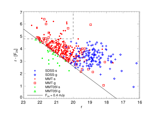
Figure 8: The comparison of different subsamples in terms of their MIR to optical [r - [F₂₄]]colors: SDSS (blue), MMT (red), and MMT05-faint (green). In grey we mark the 24 $\mu$m flux limit of 400$\mu$Jy. Objects with point source morphology are the blue pluses (SDSS), red dots (MMT), and green dots (MMT05f); extended sources are marked by blue diamonds (SDSS), red squares (MMT), and green triangles (MMT05f). The morphologies are defined by the extendedness of the SDSS optical photometry, see § 2.7.1. The different subsamples show similar MIR to optical colors within the range of [2, 4.8]. At $r>20$, a very red population of MIR-selected quasars emerges (dashed region, $r>20$, $r-[S_{24}]>4.8$), comprising a small fraction of 29 objects (14%) out of the 212 $r>20$ MIR-selected quasars.

In Fig. 8 we compare the optical to MIR colors against $r$ magnitude for the MMT and SDSS subsamples. The MIR-selected MMT subsamples are redder in $r-[S_{24}]$ colors than the SDSS subsample, with median $[r-[S_{24}]]$ values of 4.0 for MMT09, 3.9 for MMT05b, and 3.3 for SDSS. Though separable by $S_{24}$ flux, the 17 MMT05f quasars ($60<S_{24}<400\,\mu$Jy) show similar $r-[S_{24}]$ colors to the SDSS subsample, but are bluer (median $r-[S_{24}]=3.4$) than the MMT subsamples. A K-S test gives a probability of 0.975 of the MMT05f and SDSS objects, indicating identical distributions. Instead, the K-S test probability is $<0.001$ between MMT05f and the brighter MMT subsamples (MMT09, MMT05b), indicating significant difference in the optical-IR color $r-[S_{24}]$. At $r>20$, we also notice a very red population ($r-[S_{24}]>4.8$) of MIR-selected quasars (inside the dashed line, Fig. 8). The emerge of such population may simply be a result of the fainter magnitudes MMT sample covers, though this red population is still rare, which comprises 14% of the $r>20$ MIR-selected quasars (32 out of 218). The absolute i band magnitude ($M_{i}$) for the red objects has a mean $M_{i}$ of -23.6, one dex lower than the mean for the whole MIR-selected population ($M_{i}=-24.7$).

We further examine the SDSS and MMT subsamples in the luminosity-redshift space (Fig. 5). The majority (66%) of the newly identified MMT quasars are fainter than the SDSS magnitude cut of $i=20.2$. A total of 93 MMT quasars also meet the SDSS magnitude limit ($i<20.2$), which almost doubles the number of SDSS quasars in this region. One MMT source (2009.0131-268) at $z=$ 3.537 has an extremely high luminosity at $M_{i}=-29.97$. Such high luminosity is also rare in the SDSS catalog, only 82 quasars (0.078%) in the 105, 783 SDSS DR7 quasars are at $M_{i}$ brighter than -29.9. This quasar has consistent magnitudes at $i=17.5$ in modeled, fiber- and Petrosian SDSS magnitudes, but was missed in the SDSS DR7 quasar catalog for unknown reasons. The number densities of $z<3$ quasars is $\sim$ 10 deg^-2 at $i<19.1$, slightly higher than the $\sim$9 deg^-2 at $19.1<i<20.2$. The majority (78) of the new quasars are at $19.1\leq i<20.2$ and $z<3$, a region the SDSS selection deliberately avoided to ensure the selection of high $z$ targets in their $griz$ colors selection. At first glance this appears to be a major challenge to the SDSS’s claim of 90% completeness to $i_{\rm AB}=20.2$. In the following section we will explore the reasons for this inconsistency.

2.7 MIR Additions to the SDSS Quasar Selection

The MIR-selected quasars are BEL (type 1) objects satisfying the joint limits of $r<22.5$ in the optical and $S_{\rm 24}>400\mu$Jy in the MIR. The limit of $r<22.5$ is roughly equivalent to $i<22.4$ at $z\sim 1.5$ according to the Richards et al. (2006b) SED template. In Fig. 5, 93 new quasars have been identified by the MMT spectroscopy above the SDSS DR7 quasar sample limit ($i\leq 20.2$), of which 87 also satisfy the SDSS magnitude limit of M${}_{i}<-22$. Another 6 quasars are identified by re-examining the SDSS spectra. In this section we study why these objects were missed by the SDSS quasar catalog, and which additional objects the MIR selection is adding to the overall quasar population.

2.7.1 Comparing the Selection Criteria

The SDSS spectroscopic targets are selected primarily via color-selection with the SDSS photometry (Richards et al., 2002a, R02), which includes the two main low-$z$ $ugri$, high-$z$ $griz$ color selections, and a few other selections in the color-color or color-magnitude space: a mid-$z$ (2.5 $<z<$3), two high-$z$, UVX, and $ugr$ outlier inclusion regions. The 2 main uniform color selections correspond to the two magnitude cuts at $i\leq 19.1(ugri)$ and $19.1<i\leq 20.2(griz)$, with the latter designed to recover high $z$ ($z>3$) targets only —certain conditions are set to exclude low-$z$ objects. In both magnitude bins, SDSS rejected targets that fell in the color boxes of white dwarfs, A stars, M star and white dwarf pairs. The SDSS selection also excludes objects in the 2 $\sigma$ wide region around the stellar locus, with an exception for low-$z$ resolved AGNs (Schneider et al., 2010). Therefore only in the brighter $i\leq 19.1$ bin would extended sources be included, while at fainter magnitudes ($i>19.1$), all SDSS targets are point sources. Secondary SDSS targets came from the FIRST radio source catalog (White et al., 1997) and ROSAT X-ray sources (Anderson et al., 2003). Color-color selected SDSS targets were qualified as quasars if they were spectroscopically confirmed as BEL objects or have interesting absorption features (Schneider et al., 2010).

The exclusion of extended sources in the high$-z$ $griz$ color selection was achieved via the SDSS star-galaxy morphology separation. This separation is based on comparing the small point-spread function (PSF) magnitude and the larger exponential or de Vaucouleurs magnitude resulting from their different apertures. Objects for which the difference between the point-spread function (PSF) and the modeled (exponential or de Vaucouleurs profiles) magnitudes is greater than 0.145 mag are classified as extended (‘galaxy-like’, type $=$ 3, R02); otherwise they are classified as point-source (‘star-like’, type $=$ 6, R02) .

The MMT targets in the MIR quasar sample, on the other hand, are only selected based on the 24$\mu$m flux limit and r band magnitude cuts, before they are optically identified as BEL objects. The SDSS quasar selection criteria, are necessarily much more complicated given the large sky density of $i<20.2$ objects (§ 2.6). As a result, the quasar detection rate is higher for the SDSS spectra ($\sim$ 16%), than in the MMT spectra ($\sim$10%, Table. 1).

Table 3 summarizes the number counts in 3 different $i$ magnitude bins and SDSS photometric types for the SDSS and MMT quasars in this sample. We found a constant fraction of 20% of ‘extended’ MIR-selected MMT quasars in all magnitude bins, with the majority ($>$ 80%)) at lower $z$ ($<$ 1) and luminosity (log $L_{\rm bol}<$ 45.5 erg s^-1, see also § 5). These extended objects were automatically rejected in the SDSS selection at $i>19.1$. A second significant MIR addition comes from the fainter sources in the MMT surveys: a total of 160 objects are found at $i>20.2$, which SDSS did not cover.

2.7.2 MIR Additions to the SDSS Completeness

In this section we compare the colors and photometric morphologies of the SDSS and MMT identified quasars in the 3 different magnitude bins.

The SDSS uniform color selections have an estimated completeness based on simulated quasars, to be over 90% at $0<z<5.3$ down to $i=20.2$ (See also Table 6 in R02). This is an average completeness for previously known quasars, and applies to $i<19.1$ quasars at $z<2.5$, and to $i<20.2$ quasars at $3.5<z<5.3$. A later calibration of the completeness of the SDSS DR5 quasar survey gives an end-to-end completeness of $\sim$89% (Vanden Berk et al., 2005), which was confirmed in the SDSS DR5 quasar paper as “close to complete” for 0.7$<z<1.0$ and $1.9<z<2.1$ at log ($L_{\rm bol})(\hbox{erg s${}^{-1}$})>$45.9 and $>$46.6, respectively (Richards et al., 2006a; Shen et al., 2008).

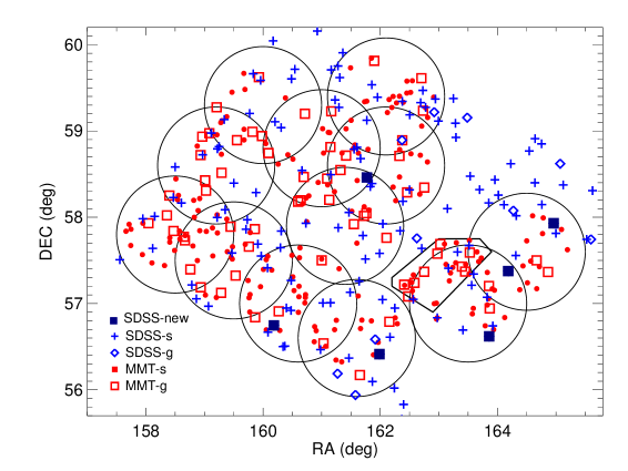
Figure 9: Quasar distribution in the LHS field: Black circles, the 12 MMT09 FOV; Black polygon, contour for the 8 MMT05 FOV; Blue pluses, point-source quasars identified with SDSS spectra (SDSS-s); Blue diamonds, extended quasars identified with SDSS spectra (SDSS-g); Red dots, point-source quasars identified with MMT spectra (MMT-s); Red squares, extended quasars identified with MMT spectra (MMT-g). Navy squares, the 6 extended quasars identified with SDSS spectra but not included in the SDSS DR7 quasar catalog (SDSS-new). For definition of the photometric morphology see § 2.7.

The distribution of quasars in the $\sim$ 22 deg² LHS field is plotted in Fig. 9. For a fair comparison, we focus only on the $\sim$12 deg² MMT covered region (within the circles and black polygon). There are a total of 96 SDSS quasars in the overlapping region (Table 3). Of these, 61 are uniformly color selected (uniform flag $=$ 1), and 29 by considering radio, X-ray, or other inclusion criteria (uniform flag $=$ 0). None of the SDSS quasars fall into the high-$z$ selected SDSS “QSO_ HiZ” branch (uniform flag $=$ 2). As mentioned in §2.6, after re-inspecting of SDSS spectra we identified 6 additional quasars not included in the SDSS DR7 quasar catalog. They are represented as dark blue squares in Fig. 5. There are 62 SDSS quasars at $i\leq\ 19.1$, 27 quasars at $19.1<i\leq\ 20.2$, and 1 at $i>20.2$. MMT observations identify an additional 13 MMT09 and 6 SDSS quasars at $i\leq\ 19.1$, of which 10 MMT09 and 4 SDSS objects qualify the SDSS M${}_{i}=-22$ limit. At $19.1<i\leq\ 20.2$, 73 MMT09 and 7 MMT05b quasars are added, of which 70 MMT09 and 7 MMT05b also satisfy M${}_{i}<-22$ (Fig. 5 and Table 3).

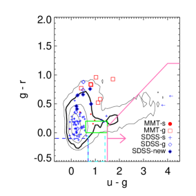
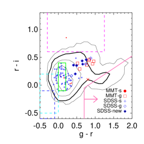
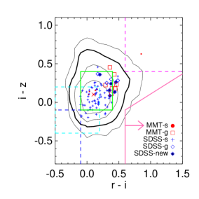
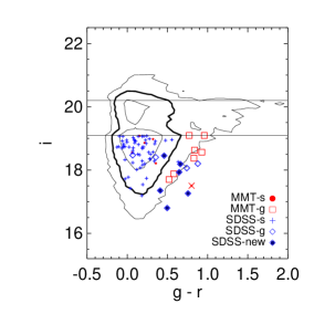
Figure 10: Location of SDSS ($blue$) and MMT ($red$) identified quasars in the SDSS colors and magnitudes diagrams for objects at $i\leq 19.1$. Symbols signals their SDSS photometric classification: blue pluses and red dots for SDSS and MMT point source (‘-s’, ‘star like’); blue diamonds and red squares for extended sources (‘-g’, ‘galaxy like’). The blue filled diamonds are the 6 newly-identified SDSS BEL objects, all of them have extended photometry. The bright MMT source (‘2009.0131-268’) is marked with a red cross in the center. Contours mark the distribution of the 110,509 SDSS DR7 quasars from Shen et al. (2011) at number densities of 20, 100, 500, and 1,000 per 0.1 magnitude or color bin. The contour level of 100 objects per 0.1 magnitude bin is highlighted as a thick line to guide the eye. For objects with $<3\sigma$ detections in either band, an upper/lower limit is used in the color-color plots. Dashed boxes are the different SDSS exclusion regions: blue for white dwarfs; $cyan$ for A stars; $magenta$ for M stars $+$ white dwarfs. Solid boxes are: $green$, the mid-$z$ inclusion regions; solid magenta with an arrow, high-$z$ inclusion regions (unique in each panel, see Richards et al. (2002a)). The black lines in the ‘g-r’ vs ‘i’ panel shows the two SDSS magnitude cuts at $i=19.1$ and $i=20.2$. About half of the MMT subsample are extended sources, mostly covered by the outmost contour level of 20 objects per bin, and 1 point MMT source falls into the SDSS M star and white dwarf exclusion region.

We first examine the bright magnitude bin of $i\leq 19.1$, where the SDSS $ugri$ color selection is optimized for low $z$ ($z<2.9$) quasar selection and includes both extended and point sources. At $i\leq 19.1$, 15% of the SDSS quasars are extended (‘galaxy-like’, see §2.7.1), while in the MMT additions, $\sim$50% are extended (Table 3). In Figure. 10, we compare the MIR-selected MMT and SDSS quasars at $i\leq 19.1$ in the 4 color-color and color-magnitude spaces. The majority of both MMT and SDSS samples fall inside the contours of 100 or more (thick curve) SDSS DR7 quasars per 0.1 magnitude bin. Only 4 of the 62 previously-identified SDSS quasars are extended (‘SDSS-g’, marked as open blue diamonds in Fig. 10). All of the 6 newly identified SDSS BEL objects (blue filled square) are extended. They were possibly rejected in the SDSS selection for being extended with blue $u-g$ colors (as indicated by vectors in Fig.4 of R02).

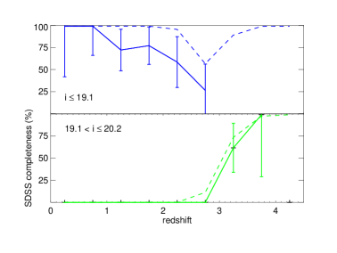
Figure 13: The observed SDSS quasar selection completeness after including qualifying MIR MMT quasars. Dashed lines plots the simulated completeness for SDSS quasars at a 0.5 redshift bin (Table 6, Richards et al. (2002a)). The SDSS completeness at $i\leq 19.1$ drops from an average 90% to ($67\pm 8$)% for the MIR-selected quasars, but is comparable at 19.1 $<i\leq$20.2.

In the bright $i\leq 19.1$ bin, 9 of the 13 new MMT09 detections satisfy the SDSS selections, including 4 point sources and 5 extended sources at $z<2.6$ (Figure. 10, Table 3). The remaining 4 MMT quasars would have been rejected in the SDSS selection, since 3 are fainter than $M_{\rm i}=-22$, and one point source falls in the SDSS M star $+$ white dwarf exclusion region (marked by magenta dashed lines in Fig. 10, See also Table 4). Despite lying at the edge of the bulk of the SDSS contours, all of the 9 new MMT objects have photometries that meet the 5$\sigma$ and error $<0.2$ requirement of the SDSS selection (R02). After adjusting for the MMT optical spectroscopy completeness (30% for MMT09, 66% for MMT05b), the overall completeness of the SDSS selection at $i<19.1$ is $(67\pm 8)\%$ (Fig. 13), about 20% lower than the simulated 90% from R02. Errors are Poisson estimates based on the inverse square root of total number of objects.

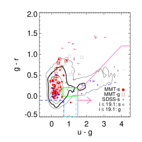
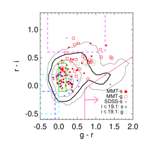
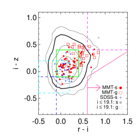
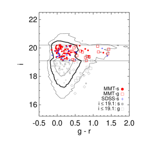
Figure 11: Colors and magnitudes of SDSS ($blue$) and MMT ($red$) identified quasars at $19.1<i\leq 20.2$ (including all redshifts). See Fig. 10 for explanation of symbols and lines. In $grey$ are the brighter objects from Fig. 10, with point sources in dots and extended sources in squares and diamonds. The MMT-subsample show a high fraction of extended sources (28%). A total of 11 MMT quasars falls in the exclusion regions: 6 in the M star and white dwarf exclusion region, of which 2 are point sources; 5 in the A star exclusion region, all of which are point sources.

In the fainter $19.1<i\leq 20.2$ bin, SDSS applied different $griz$ color cuts to select high $z$ ($>$ 2.9), point source targets. In this magnitude bin, MMT discovered 80 new objects (73 MMT09 and 7 MMT05b), the majority of which are at $z<2.9$, and are outside of the SDSS selected $z$ regions (R02). Of the 2 MMT objects that qualify the SDSS $z$ cut, only one is a point source and could have be added to the SDSS completeness analysis. Therefore, it is still valid to consider the SDSS selection complete to $\sim$90% at $z>2.9$ (Table 3). Most ($>$90%) of the low $z$ MMT quasars lie within the contours defined by the SDSS DR7 quasars and satisfy the SDSS color-color selections, though $\sim$30% of them are extended and would have been rejected had SDSS explored this low $z$ regime (Fig. 11).

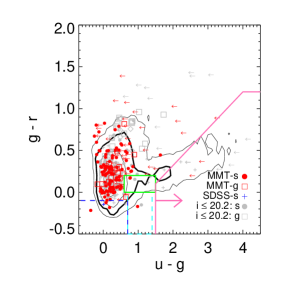
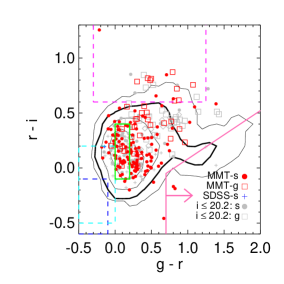
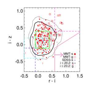
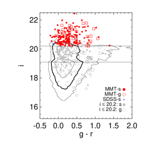
Figure 12: Colors and magnitudes of SDSS ($blue$) and MMT ($red$) identified quasars at the faint end of $i>20.2$. See Fig. 10 and Fig. 11 for for explanation of symbols and lines. In $grey$ are the brighter objects at $i\leq 20.2$. The MMT-subsample at $i>20.2$ consists of faint sources not covered by SDSS; and also shows a high fraction of extended sources (23%). A total of 25 MMT quasars falls in the exclusion regions: 4 point sources and 9 extended objects in the M star and white dwarf exclusion region; 9 point sources in the A star exclusion region; 2 point sources in the white dwarf exclusion region; and 1 point source in the white dwarf and A star overlapping region. The remaining 133 objects also qualify the SDSS color selection without $z$ or morphological cuts.

In the faintest end ($i>20.2$), which is below the SDSS quasar selection magnitude limit, only one SDSS quasar was included in the DR7 catalog (‘52411-0947-531’, not color-color selected, uniform flag $=`0$’). All of the 160 MMT quasars are newly identified objects. If compared to SDSS quasars at brighter ends ($i\leq 20.2$), the fainter targets show a large scatter in all colors (Fig. 12), including 25 MMT sources in the SDSS exclusion zones (marked by dashed lines in the first 3 panels of Fig. 12, Table 4): 13 in the M star $+$ white dwarf exclusion region, of which 9 are extended sources; 9 in the A star exclusion zone, and all are point sources; 2 in the white dwarf exclusion zone, and both are point sources; and 1 point source in the white dwarf and A star overlapped exclusion region. Two other extended objects failed the $M_{\rm i}$ cut. All of the remaining 133 targets satisfy the SDSS magnitude and $griz$ or $ugri$ color selections but not the $z$ or point-source constraints (Table 3). As at brighter magnitudes, a significant fraction (22%) of the MIR quasars are extended, of which $\sim$ 70% (25/36) lie at $z<1$.

In Fig. 13, we present the measured completeness of the SDSS quasar selections as a function of redshift, only taking into consideration the MMT objects that would otherwise satisfy the SDSS magnitude ($M_{i}<-22$), redshift ($z<$2.9 at $i<19.1$, and $z>$2.9 at $19.1\leq i<20.2$), color ($ugri$ at $z<$2.9 and $griz$ at $z>$2.9), and morphology (point source only at $i>19.1$) requirements: 9 at $i\leq 19.1$ and one at $19.1<i\leq 20.2$ (Table 3). SDSS quasar selection is close to complete at $19.1<i\leq 20.2$ and $z>2.9$, but is overestimated by $\sim$ 20% at $i<19.1$ and $z<2.9$. The modified SDSS completeness is summarized in Table 5. These values are corrected for the spectroscopic completeness of the MMT survey —numbers of MMT09 quasars are multiplied by 3.3, and by 1.5 for MMT05b objects. The corrections could be overestimated given the higher priority assigned to brighter 24 $\mu$m objects, though unlikely by a significant number, as similar detection rates are found between MMT09 (30% complete, 9.1% detection rate) and the more complete MMT05b survey (66% complete, 9.9% detection rate).

Table 3: Number counts of MIR-selected quasars identified using SDSS and MMT spectra in the overlapping regions. Second line in each magnitude bin shows the number of new objects that also satisfy the SDSS selections (see also § 2.7.2).

magnitude	$N_{\rm SDSS}$	ext	point	$N_{\rm MMT}$	ext	point	total ext
$i\leq 19.1$	(62$+$6)*	(4$+$6)* (15%)	58	13	7 (54%)	6	17 (21%)
				(9)	(5)	(4)
$19.1<i\leq 20.2$	27	0	27	80	22 (28%)	58	22 (20%)
				(1)	(0)	(1)
$i>20.2$	1	0	1	160	36 (23%)	124	36 (22%)
				(133)$\dagger$	(25)	(108)
Total	96	10* (10%)	86 (90%)	253	65 (24%)	188 (76%)	75 (21%)

Notes: Classification of the ‘extended’ (ext) and ‘point-source’ (point) morphological types are based on the SDSS photometry (§ 2.7.1). Throughout all magnitude bins, a constant 20% of the MIR quasars are extended sources. *: Six (6) are the newly-identified BEL objects with SDSS spectra not in the SDSS DR7 quasar catalog, all of which are extended. $\dagger$: For the objects which would satisfy the SDSS selection at brighter magnitudes, no redshifts or point-source cut was applied.

Table 4: Number counts of MIR-selected MMT quasars that fall in the SDSS exclusion zone.

SDSS Exclusion	$N_{\rm tot}$	point	ext
M star $+$White Dwarf	20	13	7
A star	14	0	14
White Dwarf	3	0	3

Notes: Numbers are accumulated values, for break-down in each magnitude bins, see figure captions of Fig. 10,11,12. ‘Point’ and ‘Ext’ referred to point-like sources and extended sources, respectively.

2.7.3 What makes a complete quasar sample?

Several factors contribute to the MIR additions to the quasar population and the biases in the SDSS quasar selection. Table 3 summarizes the number counts in the 2 magnitude bins in which SDSS carried out their completeness analysis. At $i\leq\ 19.1$, and $19.1<i\leq\ 20.2$, the MMT surveys add 13 and 80 additional quasars to the SDSS quasar catalog. Careful comparison reduces the numbers to 9 and 1 quasars that also qualify the SDSS selection (Table 3). If we assume a homogeneous number density across all redshifts (R02), we find the SDSS completeness is overestimated by an average 20% in $i<19.1$ quasars at $z<2.9$ (reported to be $>$ 90% in R02), but is comparable to the reported 90% for $i>20.2$ quasars at $3.5<z<5.3$ (Fig. 13). This completeness assumption is however not physical, given the known cosmic evolution of quasar number density (Hasinger et al., 2005; Silverman et al., 2008), and therefore should be used with caution. Other MIR selected samples, e.g. Lacy et al. (2013), did not show the completeness mismatch found in this paper. This is because color selections or wedges, both in optical and MIR, favor the power-law shaped SEDs (Vanden Berk et al., 2001; Richards et al., 2002a; Lacy et al., 2004; Stern et al., 2005; Donley et al., 2012), and are biased against significant host galaxy contributions, the presence of strong emission lines (e.g. PAH), and other factors such as accretion rates (Ogle et al., 2006) and LINERs (Sturm et al., 2006). In contrast, the MIR flux limit applied in this sample, selects everything above the corresponding luminosity, and therefore is not biased against dusty host galaxies or other above mentioned factors. In the whole 22 deg² LHS field, only 6 quasars in the SDSS catalog were rejected because of fainter MIR fluxes. The MIR flux-limited sample provides a complementary way to examine the quasar population as a whole, being more complete than the color selections. Of the MIR flux-limited quasars presented in this paper, the SDSS selection only recovers 58% and 10% of the total population at $i\leq 19.1$ and $19.1<i\leq 20.2$, respectively.

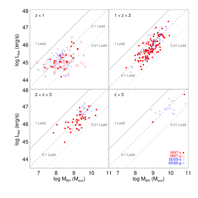
Figure 24: Bolometric Luminosity ($L_{\rm bol}$) of MIR-selected quasars as a function of SMBH mass ($\rm M_{\bullet}$). The diagonal line marks the Eddington luminosity ($L_{\rm edd}$) of corresponding $\rm M_{\bullet}$ at 1 (solid line), 0.1 (dashed line), and 0.01 (dotted line) $L_{\rm edd}$. We separate the MMT (red) and SDSS (blue) subsamples by their morphologies, pluses and filled circles for the ‘star-like’ point sources, and open diamonds and squares for the ‘galaxy-like’ extended sources (See § 2.7). The MMT quasars have lower $L_{\rm bol}$ and $\rm M_{\bullet}$ than their SDSS counterparts at $z<3$.

A significant fraction (50% at $i\leq 19.1$, and 28% at $19.1<i\leq 20.2$) of the newly identified MMT quasars are extended sources (Table. 3). SDSS chose not to include extended sources at $i>19.1$ to avoid the contamination of very red, extended objects. Their choice was based on the observation that at $z\geq 0.6$, the majority of quasars are point sources. This point-source only selection turns out to be conservative as 70% of extended targets at $i>19.1$ have a redshift higher than 0.6. Regardless of apparent magnitude, a constant fraction of 20% MIR quasars turn out to be extended sources (Table. 3), though the majority (80%) are of relatively low $z$ and luminosities ($z<1.5$, log$(L_{\rm bol})<$ 45.5 erg s^-1, Fig. 5, see also Sec 5, Fig. 24).

Another MIR addition to the sample arises from the SDSS cut of low $z$ sources in the $19.1<i\leq 20.2$ bin (Fig. 5). Because of this redshift cut, a significant number of quasars are missed from the sample, as the number density of $z<3$ quasars at $19.1<i<20.2$ is $\sim$ 24 deg^-2 (corrected for spectroscopic completeness), more than doubles the $\sim$ 10 deg^-2 found at $i<19.1$. Since the MMT09 survey is 30% complete (§2.3) and MMT05 66% complete (§2.4), on top of the 80 newly identified MMT quasars, roughly 174 quasars may remain undetected at $19.1<i\leq\ 20.2$. The majority (90%) of the MMT quasars that fall in this $z<3$ region also satisfy the SDSS color selections.

The third MIR addition is the extension to faint targets ($i>20.2$) (Table. 3). The faint MIR quasars almost doubled the number of known quasars in this field, and the majority (80%) also satisfy the SDSS color selections. The completeness corrected number density of $z<3$ quasars at $i>20.2$ is $\sim$ 45 deg^-2.

Finally, since the MIR selection does not avoid specific color areas, such as the SDSS exclusion regions of white dwarfs, M stars, and A stars, a total of 37 MMT quasars have been recovered (Table 4). They contribute to $\sim$10% of the total MIR quasar population. This is the fourth MIR addition to the SDSS quasar selection criteria.

Table 5: Observed SDSS completeness of MIR-selected quasars.

Apparent magnitude				Redshifts
	0-0.5	0.5-1	1-1.5	1.5-2	2-2.5	2.5-3	3-3.5	3.5-4
$i\leq 19.1$	100.0	100.0	72.8	77.8	59.1	26.8	…	…
	( 100.0	100.0	100.0	100.0	96.3	57.2	89.9	99.8 )
$19.1<i\leq 20.2$	…	…	…	…	…	…	62.3	100.0
	( 0.0	0.0	0.0	0.0	0.0	11.4	74.2	98.4 )

Notes: Numbers are in percentage. In parenthesis is the SDSS simulated completeness from Table 6 in Richards et al. (2002a).

Table 6: Number of Gaussians used in fits with and without an F-test.

Emission line	$N_{\rm Gaussian}$	$N_{\rm obj}$	$N_{\rm obj}$
		without F-test	with F-test
CIV	1	30 (21%)	34 (24%)
(143)	2	33 (23%)	66 (46%)
	3	80 (56%)	43 (30%)
MgII	1	75 (26%)	201 (71%)
(285)	2	50 (18%)	77 (27%)
	3	160 (56%)	7 (2%)
H$\beta$	1	8 (10%)	70 (94%)
(75)	2	66 (88%)	4 (5%)
	3	1 (2%)	1 (1%)

Table 7: Wavelength ranges used for spectral measurements in rest frame.

Emission line	redshift range	Continuum ($\AA$)	Fe Template	Emission ($\AA$)
CIV	1.63 $<z<$ 4.39	[1445, 1465] & [1700, 1705]	…	[1500,1600]
MgII	0.43 $<z<$ 2.10	[2200, 2700] & [2900, 3090]	VW01	[2700, 2900]
H$\beta$	$z<0.76$	[4435, 4700] & [5100, 5535]	BG92	[4700, 5100]

Notes: The redshift ranges are the MMT & SDSS accessible ranges based on their secure spectral ranges (See § 2.6). VW01, Vestergaard & Wilkes (2001); BG92, Boroson & Green (1992).

3 MEASUREMENTS of SPECTRA

Different virial SMBH mass ($\rm M_{\bullet}$) estimators have used different line width parameters, with either FWHM (‘full-width-half-maximum’, in km s^-1) or line dispersion, i.e., the second moment of the emission-line profile. FWHM is easier and more straightforward to measure, but can be easily overestimated in cases of line blending or extended wings. Line dispersion ($\sigma_{l}$), on the other hand, has relatively lower uncertainties, but may be overestimated for specific line profiles. Unfortunately, both parameters are affected by measurement errors, and can provide unreliable estimates for low S/N ($<$10) spectra (Denney et al., 2013). This problem can be circumvented via model fits, and Gaussian functions are widely used to fit the BELs. All the BH mass estimators we use later (MC04, VP06, VO09, and S11) are based on either one or both the FWHM and $\sigma_{l}$ of the emission line. The line dispersion $\sigma_{l}$ is arguably more reliable, given its better consistency between different lines (Park et al., 2013; Denney et al., 2013), and its better scaling to the widely used empirical $\rm M_{\bullet}-\sigma_{*}$ relation (Tremaine et al., 2002). Because the line broadening can be due to several components, a straightforward measurement of $\sigma_{l}$ is complicated, and for this work we decided to use the FWHM of the continuum subtracted emission line as the line width proxy. For a Gaussian, the FWHM has a simple correlation with $\sigma_{l}$, as FWHM $=2\sqrt{2ln2}\sigma_{l}$, or 2.35 $\sigma_{l}$. If only one Gaussian is used then the FWHM and $\sigma_{l}$ will be linearly correlated. If multiple Gaussians are used, the $\sigma_{l}$ will give a higher equivalent value than the dominant FWHM. We do provide the $\sigma_{l}$ measurements in the machine-readable table.

We wrote an IDL procedure that first measures and subtracts the continuum, and then fits one or more Gaussian profiless to the emission line. The procedure is based on the code used for the SDSS quasar catalog (S11), but includes more generality. In the cases where a single Gaussian is not a good fit to the line profile, up to 3 Gaussian components are allowed. An F-test is used to evaluate the need for each additional component. The F-test is widely used to compare the best fits of different models based on least squares comparison and the F distribution. The F value is computed as:

$$F=\frac{\chi^{2}-\chi_{\rm new}^{2}}{\rm DOF-DOF_{new}}/\frac{\chi_{\rm new}^{2}}{\rm DOF_{new}},$$ (1)

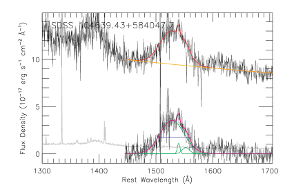
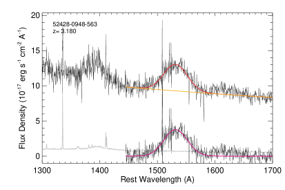
Figure 14: Example of comparison of the CIV BEL fitting results with and without an F-test (smoothed over 2 pixels). Top panel shows the SDSS results from Shen et al. (2011), where no F-test was used and the emission line was fitted with 3 Gaussian components; Bottom panel shows the same object, since the F-test shows a confidence level of 0.984, we abandoned the additional Gaussian component and kept only a single Gaussian for the BEL profile. Same color codes as in S11 are used to guide the eye. Upper and lower black lines in each panel show the original and continuum-subtracted spectra. The gray line in the lower spectra is the flux-density errors. In orange is the continuum, covered by the composite spectra in red except for the emission line region. In green are the broad Gaussians used for the BEL (covered by the composite spectra in the bottom panel). The composite spectra of the emission line is in magenta. The S11 has a dominant Gaussian FWHM of 9728 $\pm$ 506 km s^-1 , which is consistent with our results of 9409 $\pm$ 282 km s^-1 . The equivalent width (EW) results are also consistent (S11: 21.7 $\pm$ 1.4; this work: 20.3 $\pm$ 1.4). The additional Gaussian components in the SDSS fits are not necessary for this object.

where DOF is the number of degrees of freedom for the variance (“Numerical Recipes”, Second Edition,, 1992). We compute the F-test values using the IDL mpftest program. In each case, we allow up to 3 Gaussians for the BEL and use an F-test confidence level of 0.999 as the threshold. Only in cases where the F-test threshold is met, which means the new fit is significantly different from the old one, will the extra broad component be kept. Fig. 14 shows the fitting results of the same object with and without an F-test. This procedure differs from the SDSS approach, where as long as the new $\chi^{2}$ is smaller, an additional Gaussian component is added. Since the use of Gaussian profile(s) has no physical basis, we argue that the number of Gaussians should be minimized except in special cases (BALs & NALs, see Section. 7).

The introduction of an F-test significantly decreases the number of Gaussian components needed for the emission line fits (Table 6). The percentage of objects that need more than one Gaussian component drops significantly from 94% to 6% for H$\beta$; and from 74% to 29% for MgII. However, for CIV, this percentage remains high at 76%, partly due to the frequently observed asymmetry in the highly ionized CIV BELs.

We measure the FWHMs in the quasar optical spectra for the main BELs: H$\beta$, MgII, and CIV. First, the continuum is fitted with a power-law to the emission line-free region (Table 7). FeII can be strong and broad due to many multiplets, especially in the vicinity of MgII and H$\beta$ lines. Therefore the FeII emission template is also used in the continuum fit for MgII and H$\beta$. The continuum fit wavelength windows are chosen such that there is no contamination from the tail of the BEL component. We adopt the optical FeII template from Boroson & Green (1992) for H$\beta$ , and the UV FeII & FeIII templates from Vestergaard & Wilkes (2001) for MgII. No iron template is used for CIV, since the iron emission is generally weak in the CIV band. For H$\beta$ and MgII, the continuum and iron removal could be S/N dependent. In cases where the S/N of the spectra is limited (average S/N per pixel$<4$), the iron line removal is not feasible, and for these objects we only fit a power-law continuum. This affects only 3% of the objects with a MgII fit, and 8% of the objects with an H$\beta$ fit.

Up to 5 parameters are fitted simultaneously for the continuum: continuum normalization (A_λ) and continuum slope ($\alpha_{\lambda}$); for H$\beta$ and MgII, FeII template normalization (A_Fe), FeII Gaussian line-width ($\sigma_{Fe}$), and FeII velocity offset (${\rm v_{off}}$) relative to the redshift. We then fit up to 3 Gaussians to the emission lines allowing for velocity offsets (BEL central wavelength), linewidth (FWHM & $\sigma_{l}$), and equivalent width (EW) measurements. Each Gaussian is fitted with 3 parameters: maximum value (factor), mean value (central $\lambda$), and standard deviation ($\sigma$). In the case of broad or asymmetric emission lines where multiple Gaussian components are used, we provide two sets of linewidths: the ‘dominant’ FWHM — associated with the major component with the highest intensity; and the ‘non-parametric’ FWHM — of the composite line profile. The dominant FWHM increases by an average $\sim$30% after introducing the F-test, since fewer Gaussian components are used to reconstruct the emission line profile – this will increase the derived $\rm M_{\bullet}$ (See § 4). Yet the shift is usually within or around 1$\sigma$ of the FWHM error, and therefore the dominant FWHM after F-test is in general consistent with the values without the test.

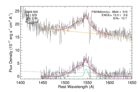
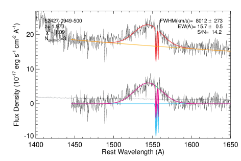
Figure 15: Example of a quasar with automatically (top) and manually (bottom) fitted CIV line profile (smoothed over 2 pixels). The manual fit accounts for the absorption feature, and better constrains the FWHM of the BEL. Upper and lower black lines in each panel show the original and continuum-subtracted spectra. The gray line in the lower spectra is the flux-density errors. In orange is the continuum, covered by the composite spectra in red except for the emission line region. In green are the broad Gaussians used for the BEL, and in cyan the absorption feature—a CIV $\lambda\lambda$4959, 5007 doublet is clearly seen redshifted from the BEL peak. The composite spectra of the emission line is in magenta.

Both narrow absorption line (NAL) and broad absorption lines (BAL, FWHM $>$ 1000 km s^-1) are commonly observed in the CIV and MgII BELs for MIR-selected quasars. NALs and BALs can affect the standard multiple Gaussian fitting algorithm and therefore need to be treated separately. If absorption features—NALs and BALs—are observed, the spectra are manually fit individually. This approach is adopted to retrieve as accurately as possible the line width measurement. Fig. 15 shows an example with absorption feature before and after the manual fit. Since the FWHMs of the emission lines are manually measured after subtracting the absorption features, they lack error bars. They will be used for $\rm M_{\bullet}$ analysis but are flagged in the catalog. More discussion can be found in § 3.4 and § 7, and in a forthcoming paper on the absorption features in MIR quasars (Dai et al., in preparation).

3.1 CIV

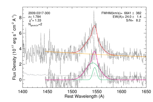
Figure 16: Example of the spectral fit for CIV BEL (smoothed over 2 pixels). Upper and lower black lines show the original and continuum-subtracted spectra. Top left shows the redshift, $\chi^{2}$ of the fit, and the number of Gaussians used in the broad line fits; top right is the fitting results of the dominant FWHM, EW, and median S/N of the emission line region. In gray is the flux-density errors. In orange is the continuum, covered by the composite spectra in red except in the BEL region. In green are the Gaussian components for the BEL. The composite spectra of the emission line is in magenta. The ‘dominant’ FWHM is from the broader Gaussian in green, while the ‘non-parametric’ FWHM is from the composite line profile in magenta. As shown in this case, the ‘dominant’ FWHM is commonly broader than the ‘non-parametric’ FWHM in 70% of the targets with multiple Gaussians.

The CIV line is fitted for the 143 objects with $1.63<z<4.40$. Iron contamination is not significant for CIV, hence, only a two parameter (A_λ, $\alpha_{\lambda}$) power-law continuum fit is used. We subtract the continuum fit to the line-free regions, and then fit the CIV emission line (Table 7). We did not subtract a narrow CIV from the line profile because it is still debated whether a narrow CIV component is present (Wills et al., 1993; Marziani et al., 1996; Sulentic et al., 2007), and to be comparable with other studies (e.g.VP06, S11, Assef et al., 2011; Park et al., 2013). For the same reason, we did not fit the 1600 $\AA$ feature, either (Laor et al., 1994; Fine et al., 2010). It is common ($>$70% ) that more than one Gaussian component is required (Table 6) to fit the $\rm CIV$ BEL profile in each of the subsamples: 48/61 for SDSS, 56/75 for MMT09, and 5/7 for MMT05b. In $\sim$ 40% of the $\rm CIV$ emission lines, NALs or BALs are seen in or adjacent to the BEL profile. Fig. 16 shows an example of a typical CIV fit.

3.2 MgII

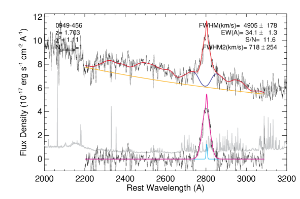
Figure 17: Example of the spectral fit for MgII BEL (smoothed over 2 pixels). Upper and lower black lines show the original and continuum and $Fe$ template-subtracted spectra. Colors and legends are explained in Fig. 16, with purple curve showing the $Fe$ template, mostly covered by the composite spectra in red except in the BEL region. In cyan is the MgII narrow emission component ($FWHM<1200\,\hbox{km s${}^{-1}$}$), whose FWHM is marked by FWHM2 in the legend.

The MgII line is fitted for the 285 objects with $0.43<z<2.10$. We adopt the iron template from Vestergaard & Wilkes (2001) and fit the continuum plus iron template to the emission-line free region (Table 7). In 9 sources with MgII coverage, the iron template is not constrained due to low spectra quality (S/N per pixel $<$ 4), in which only power-law continuum was subtracted. When the MgII emission line is fit, the MgII 2796, 2803 $\AA$ doublet ($\sim 750\hbox{km s${}^{-1}$}$ at rest-frame) is not taken into account given the much greater FWHM of the MgII emission line in all cases. As it is still debatable whether a narrow MgIIcomponent should be removed from the BEL profile (McLure & Dunlop, 2004; Vestergaard & Osmer, 2009; Wang et al., 2009), we provide two sets of measurements, (1) with and (2) without a single Gaussian for the narrow component ($<1200\,\hbox{km s${}^{-1}$}$). Objects that need multiple broad components are $\sim$ 30% (Table 6) in each of the subsamples: 25/81 for SDSS, 53/183 for MMT09, and 6/21 for MMT05b. NALs are seen in $\sim$ 8% of the objects. Fig. 17 shows an example of a typical MgII fit.

3.3 H$\beta$

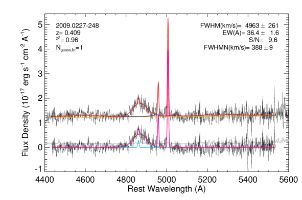
Figure 18: Example of the spectral fit for H$\beta$ BEL (smoothed over 2 pixels)s. Upper and lower black lines show the original and continuum and $Fe$ template-subtracted spectra. Colors and legends are explained in Fig. 16 and Fig. 17. In cyan is the H$\beta$, [OIII] $\lambda\lambda$4959, 5007 narrow emission components, whose FWHM is marked by FWHMN in the legend.

The H$\beta$ line is fitted for the 75 objects with $z<0.76$. We adopt the iron template from Boroson & Green (1992) and fit the continuum plus iron template in the designated spectral windows (Table 7). In 4 objects with H$\beta$ coverage, the iron template is not constrained due to the low quality of the spectra (S/N per pixel $<$ 4), and only a power-law continuum was subtracted. After subtracting the continuum and iron emission lines, we fit the [OIII] $\lambda\lambda$4959, 5007 doublets together with the H$\beta$ component. For the H$\beta$ components, we allow up to 3 Gaussians to fit the BEL, and use a single Gaussian to account for each of the narrow H$\beta$ and [OIII] emission lines. We require the narrow H$\beta$ component and the [OIII] doublets to have the same velocity shift and broadening, and constrained their FWHM to be $<$ 1200 km s^-1. Only in $<5\%$ cases do we need multiple Gaussians (Table 6) in each of the subsamples: 3/38 for SDSS, 2/31 for MMT09, and 0/6 for MMT05b. Fig. 18 shows an example of a typical H$\beta$ fit.

Table 8: Average FWHM uncertainties in our sample and comparison to literature.

Emission line	This Work	S11	VO09	VP06	P13
CIV	26%	21%	6%	9%	6%
MgII	20%	27%	10%
H$\beta$	25%	27%	12%	10%

Notes: VP06, Vestergaard & Peterson (2006), 28 quasars (reverberation mapping, RM); VO09, Vestergaard & Osmer (2009), 34 SDSS quasars and 978 LBQS quasars (single-epoch spectra, SE); S11, Shen et al. (2011), of 105,783 SDSS selected quasars (SE); P13, Park et al. (2013), of 39 AGNs (RM). The uncertainty differences arise from spectral quality and the different methods used to measure them (§3.4).

3.4 Uncertainties of Spectral measurements and Error Estimates

The uncertainties in the spectral measurement arise from three main sources: (1) the quality of the spectra and instrument errors; (2) the adopted fitting process – e.g. ambiguity introduced from using certain line profiles, and from using one or multiple components; and (3) special features that could affect the algorithm – in particular, a narrow line component, especially for MgII and CIV (cf. S11); instrumental broadening with BEL; or strong NALs or BALs.

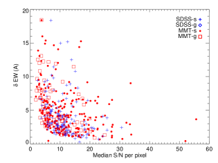
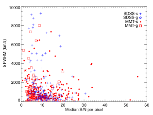
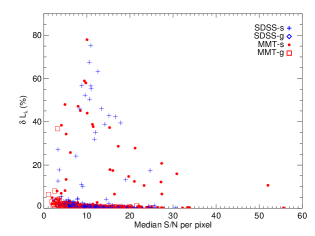
Figure 19: Uncertainties in the EW and FWHM measurements (top), and the continuum fitting results (bottom) versus the median S/N per pixel of the fitting region. Color codes are explained in Fig. 9. We observe decreasing uncertainties for EW and FWHM as the S/N of the spectrum increases, but the S/N influence on the continuum fitting is not obvious.

The fitting errors based on S/N are automatically accounted for through our IDL program using the IDL program $mpfitfun.pro$. This program returns the 1 $\sigma$ errors of each parameter from the covariance matrix. The quality of the spectra directly affects the fitting results. We observed similar S/N dependences as in S11. The uncertainty in the FWHM and EW measurements increases as the S/N in the line-fitting region decreases (Fig. 19, top). Little or no influence from the continuum S/N is found for the continuum fitting results (Fig. 19, bottom).

Instrumental broadening is not a problem for the BEL. Hectospec has a spectral resolution of 170 - 380 km s^-1 at the redshifts ($0<z<4$) for the sample (Fabricant et al., 2008). The SDSS has a 1.5 $\sim$ 2 times higher resolution (Abazajian et al., 2009). For the BELs, $\sim 99\%$ have FWHM $>2000\,\hbox{km s${}^{-1}$}$, so the instrumental resolution correction is negligible. However, the instrument resolution is comparable to the NAL widths observed (a few hundred km s^-1), so that instrumental broadening must be removed. We used the formula: $FWHM_{\rm measured}^{2}=FWHM_{\rm intrinsic}^{2}+FWHM_{\rm instrument}^{2}$ to correct the observed line-width for narrow absorption lines. The non-Gaussian flat-topped fiber profile of MMT Hectospec (Fabricant et al., 2008) renders this correction imperfect, and will be discussed in the absorption paper (Dai et al., 2014).

We adopt the Monte Carlo flux randomization method as in the SDSS routine (S11). This approach provides a more reasonable estimate than from the program fit alone, as it also smoothes out the ambiguity of whether or not to subtract a narrow line for CIV or MgII BELs. We generate 50 mock spectra with the same wavelength and flux density error arrays as the original spectrum, and randomly scatter the flux values with Gaussian noise (allowing negative values) based on the original errors. We then apply the same fitting procedure described in § 3. The measurement uncertainties are defined as the standard deviation of the measured parameters in the 50 mock spectra. This uncertainty is on average 2.1, 2.9, and 3.6 times larger than the fitting errors in FWHM for H$\beta$ , MgII , and CIV , respectively. The average FWHM uncertainties are summarized in Table 8. The uncertainties given in VP06 were adopted as the largest fitting error from their five continuum settings and could be underestimated, as the single fitting error is on average 2-3 times lower than using the Monte Carlo method. The average scaling factor between single fit and Monte Carlo uncertainties is then used to scale the uncertainties of FWHM and EW in $\sim$100 lines with strong absorption features.

The errors in FWHM and continuum measurements will directly affect the final SMBH mass (§ 4). A 50% uncertainty in FWHM translates to a 25% uncertainty in SMBH mass. In general, the flux density and spectral measurement errors are in the range of 20$\sim$30%. For the SDSS subsample, our error estimates in general agree with the SDSS results.

Table 9: Frequently Used Virial Black Hole Mass Estimators.

Emission Line	Continuum $\lambda\,(\AA)$	a	b	Reference
H$\beta$	5100	0.672	0.61	MD04
…	…	0.910	0.50	VP06
MgII	3000	0.505	0.62	MD04
…	…	0.860	0.50	VO09
…	…	0.740	0.62	S11
CIV	1350	0.660	0.53	VP06

Notes: MD04: McLure & Dunlop (2004); VP06: Vestergaard & Peterson (2006); VO09: Vestergaard & Osmer (2009); S11: Shen et al. (2011). In bold fonts are the sets of estimators we used for the fiducial SMBH mass.

4 Virial Black Hole Masses

The SMBH mass is one key property in studying the SMBH-host connection. Among the various $\rm M_{\bullet}$ estimators (e.g. Kormendy & Richstone, 1995; Gebhardt et al., 2000; Marconi & Hunt, 2003), the virial mass estimate is one of the simplest and most adopted (e.g. Kaspi et al., 2000; McLure & Dunlop, 2004; Vestergaard & Osmer, 2009). The virial method is a powerful tool especially in the absence of host galaxy information, where stellar velocity dispersion or bulge luminosity is missing. The virial method is based on the assumption that the dynamics in the vicinity of the nucleus, the ‘Broad-Emission-Line-Region’ (BLR), is dominated by the gravity of the SMBH, so that the mass of the central SMBH can be estimated from the virialized velocity of the line-emitting gas. The virial method based on the emission lines are calibrated by reverberation mapping (RM) results, which use time delays measured from the BEL variability (e.g. Vestergaard & Peterson, 2006; Wang et al., 2009; Park et al., 2013). In the RM method, the BLR radius can be measured via the light travel time delayed response of the emission line flux to continuum variation. However, only a few dozen objects have reliable RM masses due to the demanding exposure and signal-to-noise (S/N) requirements (Denney et al., 2013). The virial method is more commonly used as it requires only single-epoch (SE) spectra. For SE spectra, the BEL line-width is used as direct proxy for the SMBH mass, based on the assumption that the BLR radius is proportional to the luminosity—the observed R-L relationship (VP06; Collin et al., 2006; Bentz et al., 2009)— and the BEL line-width is proportional to the Keplerian velocity of the accreting gas.

The virial mass estimators for SMBH based on SE spectra are usually expressed as:

$${\rm log}(\frac{\rm M_{\bullet}}{\rm M_{\sun}})=a+b\,{\rm log}(\frac{\lambda L_{\lambda}}{10^{44}\hbox{erg s${}^{-1}$}})+c\,{\rm log}(\frac{\rm FWHM}{\hbox{km s${}^{-1}$}})$$ (2)

where $\rm M_{\sun}$ is the solar mass. The term $\lambda L_{\lambda}$ is the continuum luminosity, a proxy for the BLR radius (Kaspi et al., 2000; Bentz et al., 2006, 2013). They are measured from chosen wavelengths close to each BEL (Table 9). The coefficients $a$ and $b$ are empirical values based on the SMBH masses from RM and comparison among different lines. $c$ normally has a fixed value of 2. Since the BEL line-width (FWHM) represents the virial velocity, this 2 factor exemplifies the virial nature of the BLR ($\rm M_{\bullet}\propto Gv^{2}R^{-1}$). Recently a few papers have suggested using other values for $c$ based on comparison of SE and RM results. For instance, Wang et al. (2009) used 1.09 and 1.56 in front of the H$\beta$ and MgII FWHMs, respectively. Park et al. (2013) used 0.56 in front of the CIV FWHMs. If a $<2$ factor is adopted, the resulting SMBH mass estimate will be smaller accordingly. Here we stick to the $c=2$ value to be consistent with the SDSS quasar catalog (S11).

The CIV, MgII, and H$\beta$ BELs are widely used as virial black hole mass calibrators (e.g. McLure & Dunlop, 2004; Vestergaard & Peterson, 2006; Vestergaard & Osmer, 2009; Shen et al., 2011). We summarize the most frequently used virial estimators in Table 9. If multiple Gaussian components are used, in the catalog we provide both the dominant and the non-parametric $\rm M_{\bullet}$ derived from the dominant and non-parametric FWHM. In the following analysis of $\rm M_{\bullet}$ properties, for the MgII and H$\beta$, we use the $\rm M_{\bullet}$ derived from the non-parametric FWHM to be consistent with the literature definitions. This choice of non-parametric FWHM in general provides lower $\rm M_{\bullet}$ estimates than from dominant FWHM, and may underestimate the $\rm M_{\bullet}$ for BELs if the emitting gas is in Keplerian motion.

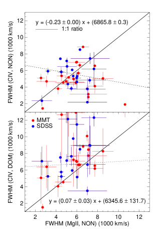
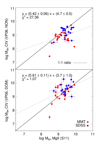
Figure 20: (left) Comparison of the non-parametric (top) and dominant (bottom) CIV FWHM against the non-parametric MgII emission line width. (right) SMBH mass ($\rm M_{\bullet}$) in $\rm M_{\sun}$ derived from the non-parametric (top) and dominant (bottom) CIV FWHM against the $\rm M_{\bullet}$ from the non-parametric MgII FWHM. In each pane, diagonal line marks the linear correlation (See § 4). The MIR-selected MMT targets are in red and the SDSS targets in blue. The dominant CIV FWHMs are systematically higher than the non-parametric CIV FWHM in 70% of the cases with multiple Gaussians (See, e.g., Fig. 16), and has a marginally smaller scatter from the1:1 linear correlation with the MgII non-parametric FWHM. A better correlation to the MgII derived $\rm M_{\bullet}$ is also observed of the $\rm M_{\bullet}$ from dominant CIV FWHM (linear fit slope: $0.61\pm 0.11$) than from the non-parametric CIV FWHM (linear fit slope: $0.42\pm 0.06$), possibly indicating a non-virial component in the CIV BEL.

For the CIV calibrator, the line-width definition in literatures is also the same as the non-parametric FWHM (VP06, see also Peterson et al., 2004). However, it is debated as to whether it provides a reliable $\rm M_{\bullet}$ estimate due to the large scatter between the generally consistent CIV and H$\beta$ derived $\rm M_{\bullet}$ (Netzer et al., 2007; Assef et al., 2011). This scatter may result from non-virial components from outflows or winds in the CIV BLR (e.g. Richards et al., 2011). For this MIR-selected quasar sample, we find a marginally better correlation between the dominant CIV FWHM and the non-parametric MgII FWHM (Figure. 20, left). Better consistency is also found between the $\rm M_{\bullet}$ derived from the dominant CIV component and MgII BELs (Figure. 20, right), indicating a non-virial contribution in the non-parametric BEL profile. Based on the correlation results, we choose to use the dominant CIV FWHM for $\rm M_{\bullet}$ estimates. We will discuss the choice and its implications in § 7.

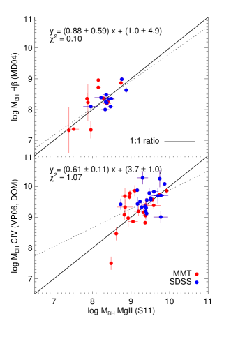
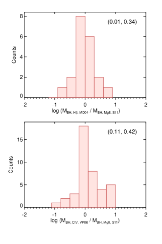
Figure 21: (left): Comparison of SMBH masses in $\rm M_{\sun}$ derived from different lines for the quasars with both H$\beta$  and MgII (top), MgII and CIV (bottom) BELs. MMT sources are marked in red and SDSS sources in blue. A median line S/N per pixel $>$ 5 was required. Diagonal line marks the 1:1 correlation, and dashed line marks the best fit linear correlation. The best-fit coefficient and associated errors are marked at the top left corner. The $\rm M_{\bullet}$ from S11 (MgII) estimator shows a tight correlation with the $\rm M_{\bullet}$ from MD04 (H$\beta$), and is consistent with the $\rm M_{\bullet}$ from VP06 (CIV). (right): The mass ratio distributions for the two sets of estimates for the same object. A median line S/N per pixel $>$ 5 was required. The mean and 1$\sigma$ from a Gaussian fit to the distribution are plotted at the top right corner.

In our catalog, if applicable, we present multiple $\rm M_{\bullet}$, using MD04 (H$\beta$, MgII), VP06 (H$\beta$, CIV), VO09 (MgII), and S11 (MgII) estimators. We attribute the $\rm M_{\bullet}$ from MD04 (H$\beta$), S11 (MgII), and VP06 (CIV) as the ‘fiducial’ $\rm M_{\bullet}$ to each object, as the $\rm M_{\bullet}$ from these parameters are best-correlated with each other (Fig. 21, left). We compare the different estimators based on the subsample of quasars that have two BELs with a median S/N per pixel of $>$ 5 and no BAL/NAL, which leaves 20 objects with both MgII and H$\beta$ BELs, and 38 targets with both CIV and MgII BELs. The comparison of the $\rm M_{\bullet}$ from different lines and estimators for quasars with two BELs is achieved by forcing a linear correlation and measuring the $\chi^{2}$ values to compare the sample scatter.

We first compare the three MgII estimators (MD04, VO09, S11) with the CIV estimator (VP06), and found a marginally smaller $\rm M_{\bullet}$ scatter for VP06 (CIV) & S11 (MgII) ($\chi^{2}=1.07$) than for VP06 (CIV) & VO09 (MgII) ($\chi^{2}=1.07$). Both have a $\chi^{2}$ value $\sim$1 dex better than VP06 (CIV) & MD04 (MgII). The slope coefficient in all three sets of estimators agree with each other within errors at a value $\sim$0.6. The scatter in log$(M_{\rm BH},{\rm CIV,(VP06)}/M_{\rm BH},{\rm MgII,(S11)})$ is similar to the scatter for the SDSS DR7 catalog (see Fig.10, S11). This small scatter between S11 and VP06 is by design, as the S11 coefficients were empirically adopted to provide the best correlation between VP06 (CIV) and S11 (MgII) results. For ease of comparison with the SDSS sample, we assign the $\rm M_{\bullet}$ from S11 as the fiducial $\rm M_{\bullet}$ from MgII BEL.

We then make the same $\chi^{2}$ comparison for the two H$\beta$ estimators (VP06, MD04) and the chosen MgII estimator S11. For the same H$\beta$ BEL, $\rm M_{\bullet}$ from VP06 is systematically 0.2 dex higher than from MD04, since the VP06 ‘a’ factor is $\sim$0.2 larger (Table 9). S11 & MD04 show a slightly smaller scatter ($\chi^{2}$ = 0.59) than S11 & VP06 ($\chi^{2}$ = 0.78), so $\rm M_{\bullet}$ from MD04 is chosen as the fiducial $\rm M_{\bullet}$ in H$\beta$ BELs. The scatter in log$(M_{\rm BH},{\rm H\beta,(MD04)}$ / $M_{\rm BH},{\rm MgII,(S11)})$ is also similar to that of the SDSS DR7 catalog (see Fig.10, S11).

In summary, for the MIR-selected sample, we find that MD04 (H$\beta$), S11 (MgII), and VP06 (CIV) show the best correlations and assign a fiducial $\rm M_{\bullet}$ using these three estimators. If $\rm M_{\bullet}$ from MgII and H$\beta$ BELs are both available, the $\rm M_{\bullet}$ derived using H$\beta$ will be adopted as the fiducial $\rm M_{\bullet}$ because of the robust SE mass scaling from H$\beta$ RM studies. For targets with $\rm M_{\bullet}$ from both CIV and MgII BELs, we attribute the MgII  derived $\rm M_{\bullet}$ given the possible complications of non-virial component from the CIV BELs.

In Fig. 21 (right), we plot the mass ratios distribution for the quasar subsample with 2 BELs (median S/N per pixel of $>$ 5). The mean and 1$\sigma$ from a Gaussian fit to the mass ratio distributions are (0.01, 0.34) for log $(M_{\rm BH},{\rm H\beta,(MD04})/M_{\rm BH},{\rm MgII,(S11}))$ and (0.11, 0.42) for log $(M_{\rm BH},{\rm CIV,(VP06})/M_{\rm BH},{\rm MgII,(S11}))$. The mean offsets are negligible since they are smaller than what a typical FWHM error would introduce: a 30% error in FWHM translates to an upper and lower uncertainty of $+$0.11 dex & $-$0.15 dex in the log ($\rm M_{\bullet}$) space, and justifies the choice of these three estimators.

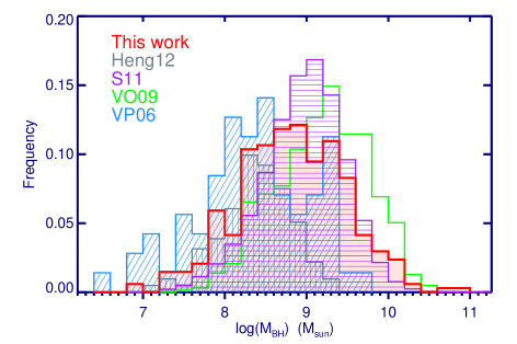
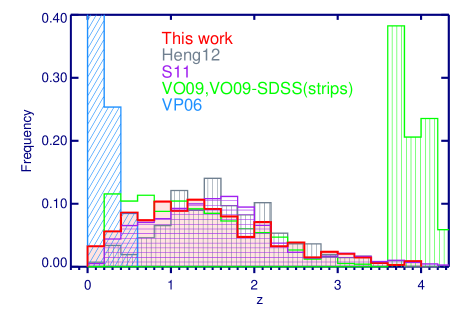
Figure 22: (top) BH mass distribution of the relative frequency of the 391 MIR-selected quasar sample (red). Literature values from SDSS and other surveys are also plotted for comparison: gray, 413 X-ray selected quasars (Heng et al., in prep), purple,105,783 SDSS selected quasars (Shen et al., 2011, S11), blue, 1,012 $z<5$ quasars, including 34 SDSS quasars at 3.5$<z<$5 (Vestergaard & Osmer, 2009, VO09), green, 71 $z<0.3$ quasars with reverberation mapping info (Vestergaard & Peterson, 2006, VP06). (bottom) Redshift distribution of the MIR-selected quasars (red). Samples from the literature are color-coded in the same way as the top panel. The MIR-selected quasar sample overlaps with Heng12, S11, VO09-BQS, LBQS quasars in redshifts, and has a large overlap in $\rm M_{\bullet}$ with the SDSS quasars. VP06 extends to the low mass end partly due to their relatively lower redshift from the RM constraint.

We show the SMBH mass and redshift distribution for the MIR-selected quasar sample in Fig. 22, and superpose samples from the literature for comparison. The redshift distribution of the MIR-selected quasars is typical of an apparent-magnitude limited sample, and has a large overlap with the SDSS, BQS, and LBQS catalogs. For $\rm M_{\bullet}$, the MIR-selected sample also overlaps with the above mentioned samples, but have a higher fraction of lower mass objects than the S11 sample—a direct result of the fainter magnitude limit applied.

5 Bolometric Luminosity and Eddington Ratios

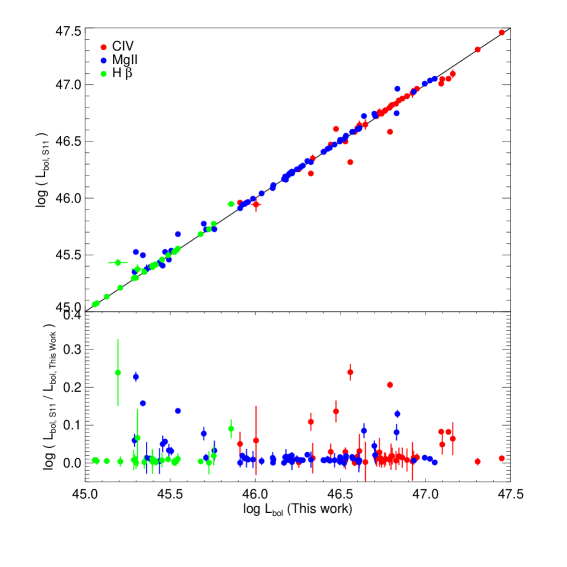
Figure 23: The bolometric luminosities ($L_{\rm bol}$, top panel) and $L_{\rm bol}$ comparisons for the same targets between SDSS DR7 and this work (bottom, panel) as a function of $L_{\rm bol}$. Only objects with a median line S/N per pixel $>3$ are included. Targets with NALs/BALs are excluded. The two independently derived $L_{\rm bol}$ are consistent with each other ($<3\sigma$) for the majority ($\sim$80%) of the MIR-selected SDSS subsample.

We measure the bolometric luminosity $L_{\rm bol}$ from the fitted spectra continuum luminosities: $L_{\rm bol}=k\times L_{\lambda}$, where $L_{\lambda}$ are $L_{5100}(z<0.76$, H$\beta$), $L_{3000}(0.43<z<2.10$, MgII), and $L_{1350}(1.63<z<3.18$, CIV) in erg s^-1; and $k=$ 9.26, 5.15, and 3.81, respectively (cf. S11). The coefficient $k$ values are from the composite SED from Richards et al. (2006b, R06), a modified SED largely consistent with Elvis et al. (1994). The R06 template should be applicable to at least the point source targets in this work, since it is based on 259 $Sptizer$ detected SDSS type 1 (BEL) quasars, and 96% (248/259) of which also qualify the MIR-selection of $S_{\rm 24}>400\mu$Jy for this sample. Therefore, we caution the usage of the cataloged $L_{\rm bol}$ and its derived parameters for extended objects. We did not correct the spectra for intrinsic extinction (See also § 2.5). This may result in $L_{\rm bol}$ being underestimated for systems with strong reddening; or overestimated if there is significant host contamination. A fourth estimator using $S_{\rm 24}$ flux shifted to the rest-frame is also introduced for comparison, in which the $k$ values differ from redshift to redshift. Given the uncertainty in the quasar MIR SED shapes (Dai et al., 2012), we caution the use of the MIR flux-derived $L_{\rm bol}$. It is on average 0.5 dex higher than the optical continuum-derived values, possibly from degenerate factors of reddening, host contamination, and possible PAH emission contamination at $z>2$. For comparison, we will only discuss the continuum-derived $L_{\rm bol}$ in the following discussion. All MIR-selected quasars have $L_{\rm bol}$ greater than $10^{44}{\rm erg\,s^{-1}}$, confirming their quasar nature (Fig. 23).

For the MIR-selected SDSS subsample, a comparison with the SDSS DR7 quasar catalog (S11) shows consistency within 3$\sigma$ in continuum-derived $L_{\rm bol}$ (Fig. 23) for over 80% of the MIR-selected targets. The MIR-selected quasars have an overall lower $L_{\rm bol}$ distribution than SDSS DR7 quasars, since they include a large fraction (40%) of objects fainter than the SDSS magnitude cut at $i>20.2$. The median fitting errors for $L_{\rm bol}$ are 2%, 1%, and 3% for the H$\beta$, MgII, and CIV BELs, respectively. In objects that fall in $0.46<z<0.76$ or $1.63<z<2.10$, where two BELs are covered, we find a $\sim$40% consistency between the $L_{\rm bol}$ from CIV and MgII, and $\sim$15% between MgII  and H$\beta$, evidence of reddening or host contribution. In the following analysis, if two $L_{\rm bol}$ are available for the same object, we use the $L_{\rm bol}$ that corresponds to the chosen $\rm M_{\bullet}$ (See § 4).

Table 10: Median SMBH mass, bolometric luminosity, and Eddington ratios of the MIR-selected quasars.

Redshift	Subsample	$\#_{\rm obj}$	$log(\rm M_{\bullet})(\rm M_{\sun})$	$log(L_{\rm bol})(\hbox{erg s${}^{-1}$})$	$log(L_{\rm bol}/L_{\rm edd})$
$z<1$	SDSS	44	8.26 $\pm$ 0.53	45.21 $\pm$ 0.40	-1.07 $\pm$ 0.53
	MMT	82	8.39 $\pm$ 0.56	45.01 $\pm$ 0.46	-1.33 $\pm$ 0.55
	overall	126	8.34 $\pm$ 0.55	45.06 $\pm$ 0.44	-1.24 $\pm$ 0.55
$1<z<2$	SDSS	55	9.05 $\pm$ 0.47	46.10 $\pm$ 0.61	-1.05 $\pm$ 0.32
	MMT	126	8.85 $\pm$ 0.44	45.72 $\pm$ 0.53	-1.14 $\pm$ 0.34
	overall	181	8.91 $\pm$ 0.45	45.81 $\pm$ 0.56	-1.10 $\pm$ 0.33
$2<z<3$	SDSS	22	9.59 $\pm$ 0.24	46.80 $\pm$ 0.36	-0.98 $\pm$ 0.32
	MMT	43	9.29 $\pm$ 0.52	46.27 $\pm$ 0.44	-1.15 $\pm$ 0.38
	overall	65	9.40 $\pm$ 0.48	46.37 $\pm$ 0.50	-1.05 $\pm$ 0.37
$z>3$	SDSS	17	9.92 $\pm$ 0.47	46.86 $\pm$ 0.28	-0.90 $\pm$ 0.44
	MMT	2	10.78 $\pm$ 1.27	47.69 $\pm$ 1.11	-0.95 $\pm$ 0.16
	overall	19	9.92 $\pm$ 0.54	46.86 $\pm$ 0.38	-0.91 $\pm$ 0.42
Redshift	Type	$\#_{\rm obj}$	$log(\rm M_{\bullet})(\rm M_{\sun})$	$log(L_{\rm bol})(\hbox{erg s${}^{-1}$})$	$log(L_{\rm bol}/L_{\rm edd})$
$z<1$	point	58	8.34 $\pm$ 0.46	45.29 $\pm$ 0.41	-1.07 $\pm$ 0.46
	ext	68	8.38 $\pm$ 0.61	44.93 $\pm$ 0.42	-1.34 $\pm$ 0.59
$1<z<2$	point	172	8.91 $\pm$ 0.45	45.81 $\pm$ 0.57	-1.10 $\pm$ 0.34
	ext	96	8.90 $\pm$ 0.34	45.95 $\pm$ 0.35	-1.24 $\pm$ 0.24
$2<z<3$	point	61	9.44 $\pm$ 0.48	46.40 $\pm$ 0.49	-1.05 $\pm$ 0.38
	ext	4	9.12 $\pm$ 0.26	45.94 $\pm$ 0.49	-1.25 $\pm$ 0.24
$z>3$	point	19	9.92 $\pm$ 0.54	46.86 $\pm$ 0.38	-0.91 $\pm$ 0.42
	ext	…	…	…	…

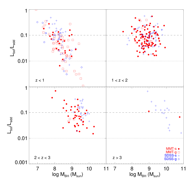
Figure 25: Eddington Ratios ($L_{\rm bol}/L_{\rm edd}$) of MIR-selected quasars as a function of SMBH mass ($\rm M_{\bullet}$). Color codes and legends are the same as in Fig. 24. The dashed and dotted lines mark the 0.1 and 0.01 Eddington ratios, respectively. At $z<1$, the extended sources show clearly lower $L_{\rm bol}$ ($\sim$ 0.7 dex) and an average of $\sim$ 3 $\times$ lower Eddington ratios than the point sources; at $1<z<2$ and $2<z<3$, where limited extended sources are available, the point sources show a wide span of Eddington ratios and scatter into the $L_{\rm bol}/L_{\rm edd}<0.1$ regime.

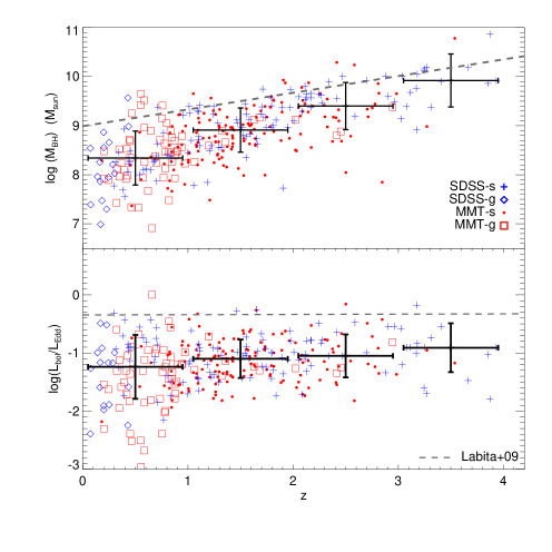
Figure 26: SMBH mass ($\rm M_{\bullet}$, top) and Eddington Ratios ($L_{\rm bol}/L_{\rm Edd}$, bottom) of MIR-selected quasars as a function of redshift. Color codes and legends are the same as in Fig. 24. In dashed lines are the proposed maximum mass values ($M_{\bullet(max)}=0.34\,z+8.99$) and Eddington ratios ($L_{\rm bol}/L_{\rm Edd}(max)=0.005\,z+0.45$) from Labita et al. (2009). The mean and standard deviation in each redshift bin is marked by black pluses. We observe a downsizing effect in $\rm M_{\bullet}$ but a more or less constant Eddington ratios across the cosmic time.

In Fig. 24, we compare the $\rm M_{\bullet}$ with $L_{\rm bol}$. The diagonal line marks the Eddington luminosity for the corresponding SMBH mass. Quasars rarely exceed $L_{\rm Edd}$ (Kollmeier et al., 2006) and SDSS quasars tend to lie above $\sim$0.05 $L_{\rm Edd}$, and below a ‘sub-Eddington boundary’ (Falcke et al., 2004; Labita et al., 2009; Steinhardt & Elvis, 2010). Controversies exist as to whether the observed sub-Eddington limit is due to the incompleteness of SDSS sample at low $\rm M_{\bullet}$ ($\rm M_{\bullet}<3\times 10^{8}\rm M_{\sun}$) and low Eddington ratio (ER, $L/L_{\rm Edd}<0.07$) (Kelly & Shen, 2013). For the MIR-selected sample, we do not observe a clear sub-Eddington limit (Fig. 25). The $\rm M_{\bullet}$ for MIR-selected quasars shows a trend of downsizing, though the $L_{\rm bol}/L_{\rm Edd}$ is relatively independent of redshift (Fig. 26). These trends are similar to the results from the SDSS DR5 quasars (Labita et al., 2009). Table 10 summarizes the $\rm M_{\bullet}$, $L_{\rm bol}$, and $L_{\rm bol}/L_{\rm Edd}$ differences between the MMT and SDSS subsamples, and between point and extended sources. At all redshift ranges, the MMT identified quasars have a lower median $L_{\rm bol}/L_{\rm Edd}$ ratio than their SDSS counterparts, possibly related to the inclusion of extended sources in the MMT sample, since the mean $L_{\rm bol}/L_{\rm Edd}$ ratio is also lower for extended targets at all redshift.

At $z<1$, the extended sources show lower $L_{\rm bol}$ ($\sim$ 0.4 dex) and lower ER (by a factor of 2) than the point sources (Fig. 25). It is possible that the extended quasars reside in brighter or more massive host galaxies, and at a less active evolutionary phase with lower $L_{\rm bol}/L_{\rm Edd}$. Of the 12 targets with rather low ERs ($L_{\rm bol}/L_{\rm Edd}<0.01$), 10 are extended sources. Of the remaining 58 extended sources at $z<1$, 16 have a $L_{\rm bol}/L_{\rm Edd}>0.1$, and 42 are at $0.01<L_{\rm bol}/L_{\rm Edd}<0.1$. The $L_{\rm bol}/L_{\rm Edd}$ may be underestimated as quasars may contribute significantly in the rest-frame FIR as suggested by Kuraszkiewicz et al. (2003) and Dai et al. (2012). On the other hand, the ER may also be overestimated because of the possible host contribution to the $L_{\rm bol}$ at $z<1$; though the reddening correction of the spectra will counteract that effect. In the spectrum of at least a few MIR-selected SDSS sources with extended photometry, stellar absorption and sometimes a Balmer break is observed. For example, the 6 newly-identified SDSS quasars with extended morphology all show signatures of host galaxy (e.g. Fig. 6): all have CaII H&K absorption, and four (4) also show the G band in absorption.

At $1<z<3$, the MMT identified subsample has systematically lower $L_{\rm bol}$ and $\rm M_{\bullet}$ than their SDSS counterparts (Fig. 24, see also Table 10). The MMT sources extend the SDSS selection to fainter magnitudes (Fig. 5), so at a given redshift, they must either have lower $L_{\rm bol}/L_{\rm Edd}$, or of smaller $\rm M_{\bullet}$. Kelly & Shen (2013) suggested that the sub-Eddington boundary found for SDSS quasars was a magnitude-limit effect, and there was a large population of low $L_{\rm bol}/L_{\rm Edd}$ quasars down to $\rm M_{\bullet}\,\sim\,5\,\times 10^{8}\rm M_{\sun}$ (log$(\rm M_{\bullet})=8.7\,\rm M_{\sun}$) and $L_{\rm bol}/L_{\rm Edd}\sim 0.07$ (log$(L_{\rm bol}/L_{\rm Edd})=-1.15$). These do not appear in the MIR-quasar population for 1$<z<$3. Instead of a shift of the $\rm M_{\bullet}$ and $L_{\rm bol}/L_{\rm Edd}$ to smaller values, comparable mean and scatter of ERs and $\rm M_{\bullet}$ are observed at 1$<z<$2 and 2$<z<$3 (Fig. 25). At $1<z<3$, the point sources also scatter into the $<0.1\,L_{\rm bol}/L_{\rm edd}$ regime. However, given the small numbers of extended objects at $z>1$—possibly due to the resolution restrictions of the telescope—it is difficult to tell whether there is any systematic difference in the SMBH accretion rate between extended and point-like quasars at earlier cosmic time.

Table 11: Sample Entry of the basic parameters for the MIR-selected quasar sample.

ID	RA	DEC	redshift	$S_{\rm 24}$	$\delta S_{\rm 24}$	SDSS photometry
	(J2000)	(J2000)		$\mu Jy$	$\mu Jy$	(u, g, r, i, z)
2009.0131-005	162.3289	59.4024	1.650	2282.43	19.42	(21.73, 21.07, 20.69, 20.22, 19.89)

(This table is available in its entirety in a machine-readable form in the online journal. A portion is shown here for guidance regarding its form and content. Detailed catalog format can be found in Table LABEL:tab:properties. SDSS photometry errors are not shown here due to space limitation.)

Table 12: Luminosities and SMBH mass of the MIR-selected quasar sample.

ID	Flag_EXT	Flag_ABS	Flag_FAINT	log$\rm M_{\bullet}$	$\delta\rm M_{\bullet}$	log$L_{\rm bol}$	$\delta L_{\rm bol}$	$L_{\rm bol}/L_{\rm edd}$	…
				$\rm M_{\sun}$	in %	erg s-1	in %
2009.0131-005	6	1	0	9.17	0.17	46.99	0.01	0.50	…

(This table is truncated for viewing convenience. It is available in its entirety in a machine-readable form in the online journal. A portion is shown here for guidance regarding its form and content. Detailed catalog format can be found in Table LABEL:tab:results.)

Table 13: Fitting parameters of the MIR-selected quasar sample.

ID	…	CIV_ dom_ FWHM	…	MgII_ dom_ FWHM	…	H$\beta$_ dom_ FWHM	…
		km s-1		km s-1		km s-1
2009.0131-005	…	2056.6 $\pm$ 221.2	…	4773.9 $\pm$ 363.0	…	…	…

(This table is truncated for viewing convenience, only the dominant FWHM for each line is listed. Additional columns and format information can be found in Table LABEL:tab:param. It is available in its entirety in a machine-readable form in the online journal. A portion is shown here for guidance regarding its form and content. )

6 The Spectral Catalog

We have included all the measured properties from line fitting, and the derived properties in the online master catalogs. This catalog will be available in its entirety in a machine-readable form in the online journal. Objects are arranged in increasing RA order, and the ID reflects the spectroscopic subsamples: MMT09, MMT05b and SDSS. The MMT05f faint objects are then appended to the end of each table for comparison. Table 11,12, and 13 show sample entries of the three master tables. Table 11 lists all the basic parameters, including the object ID, position, redshift, SDSS and MIPS 24$\mu m$ photometries of the quasar sample; Table 12 shows a sample entry the results, including flags, luminosities, SMBH mass, and ERs; Table 13 includes the fitting parameters: continuum normalization and slope, iron template normalization and broadening, wavelength, S/N, FWHM, line area, and EW of each emission line. The catalog format can be found in Table LABEL:tab:properties, Table LABEL:tab:results, and Table LABEL:tab:param. Unless otherwise stated, a null value is given if no measurements are available.

7 Discussion

The catalog of MIR-selected quasars can be used to study the statistics of type 1 quasars and their physical properties.

We find that a significant and constant fraction (20%) of MIR-selected quasars have extended optical photometry at $z<1.5$, indicating luminous host galaxies (Table 3). The MMT-recovered quasars include a small population of redder targets than the SDSS quasars (Fig. 8). The MMT quasars share similar distributions with the SDSS quasars in all colors at $i\leq 20.2$, and cover fainter objects than SDSS did not cover at $i>20.2$ (Fig. 10,11,12). The SDSS quasar algorithm is biased towards point sources at $i>19.1$ and is therefore missing quasars residing in extended hosts. Unresolved quasars comprise about 94% of all SDSS quasars. SDSS did not include extended objects in their target selection based on the assumption that the expected yield of quasars would be low. The MIR flux limit used in this sample is more inclusive and recovers the otherwise rejected extended sources. The extended population consists of 20% of the total MIR quasar population, and calls for re-examination and updated simulations for quasar distributions at all redshifts.

Although the SDSS algorithm completeness was simulated and found to be consistent with MIR color-selected quasar samples, e.g. Lacy et al. (2013), we discovered additional quasars using the flux-limited MIR-selection. At $i>19.1$, 9 additional MIR quasars that meet the SDSS selection were recovered with the MMT spectroscopy, resulting in an updated SDSS completeness of 70%. At $i<20.2$ and $z>2.9$, we only found 1 additional MIR quasar which is consistent with the SDSS completeness of 90%. This completeness difference arises from the different selection criteria, as both optical and MIR color selections restrict the sample to power-law like SEDs, whereas the MIR flux selection adopted here includes everything that meet the apparent magnitude requirement. At $z<3$ and $i>19.1$, the observed quasar number densities per square degree are higher than at the SDSS covered $i<19.1$ region.

In Fig. 7, the MIR-selected quasars show a redshift distribution peaking at $z\sim$1.4, consistent with previous studies of the cosmic evolution of AGN number densities (Hasinger et al., 2005; Silverman et al., 2008). We see evidence of downsizing in the MIR-selected targets, with the most massive SMBHs appearing at earlier times; though the ER remains almost constant at $1<z<4$ with large scatters. Objects with low $L_{\rm bol}/L_{\rm Edd}<0.01$ are also observed at $z<1$.

Controversies exist as to whether CIV line-widths are attributed solely to gravity, or are affected by outflows or jets, and as a result, whether the CIV emission derived masses are as reliable as MgII and H$\beta$  derived masses (VP06, Shen et al., 2008; Assef et al., 2011). This concern arises from both the typically blueshifted CIV BEL peak compared to other quasars BELs (Gaskell, 1982; Richards et al., 2002b, S11), the commonly observed BAL/NALs (Weymann et al., 1981, W08) within the CIV emission line profiles, and the strong line asymmetries (Wilkes, 1984; Richards et al., 2002b, See also § 3). The blueshift of the CIV BEL peak relative MgII is observed in $\sim$80% of the MIR-quasars whose spectra covers both CIV and MgII BELs. In the MIR-selected quasar sample, there is no strong correlation between the CIV and MgII FWHMs (Figure. 20, left). There is also no strong trend of decreasing ratios of log$(M_{\rm BH,(MgII)}/M_{\rm BH,(CIV)})$ with increasing CIV$-$MgII  blueshifts, in contrast to the correlation reported in S11 & Richards et al. (2011), although the scatter is large for both $\rm M_{\bullet}$ ratios and CIV$-$MgII  blueshifts (Fig. 27).

A non-virial CIV emission component can be used to explain the large scatter observed between CIV and other BEL derived $\rm M_{\bullet}$ (S11 Richards et al., 2011; Denney, 2012). Denney (2012) found a ‘non-variable, largely core’ emission component in the CIV BEL by comparing the SE spectra to the RM spectra. After removing this non-variable component, the CIV derived $\rm M_{\bullet}$ shows a better correlation with the H$\beta$ derived $\rm M_{\bullet}$. In this MIR-selected quasar sample, we found that the $\rm M_{\bullet}$ derived from the dominant CIV FWHM shows a marginally better correlation with the $\rm M_{\bullet}$ from MgII BEL (slope coefficient $=$ 0.61 $\pm$ 0.11) than that from the non-parametric CIV FWHM (slope coefficient $=$ 0.42 $\pm$ 0.07, Figure. 20, right) and has smaller scatter. If non-parametric CIV  FWHM is used instead, a sudden jump in the $\rm M_{\bullet}$ distribution at $z\sim$ 1.6 would appear, where the $\rm M_{\bullet}$ starts to be derived from the CIV  BELs. This sudden increase is not physical and supports our choice of the dominant CIV FWHM. In 70% of the CIV BEL with multiple Gaussians, the non-parametric CIV FWHMs are smaller than the dominant CIV FWHMs, due to contributions from narrower Gaussians that fit the line core (e.g., Fig. 16). These narrower additional Gaussian component resembles the non-virial emission component found in Denney (2012, Fig.3). The marginally better correlation of dominant CIV $\rm M_{\bullet}$ to MgII derived $\rm M_{\bullet}$ suggests contamination from non-virial CIV components to the non-parametric CIV FWHM. The choice of dominant CIV FWHM instead of the conventional non-parametric FWHM for $\rm M_{\bullet}$ estimates may provide a way to tackle this problem.

We find a high fraction of objects with absorption features in the MIR-selected sample. For CIV, $\sim$40% of the BELs quasars show absorption, NALs or BALs; and this fraction is $\sim$ 20 % for MgII objects. The fraction of BALs in MIR-selected quasars, is 17$\pm\ 3\%$ in CIV, and 10$\pm$2% in MgII. The CIV numbers agree with the overall fraction of 10-15% found for SDSS quasars (e.g. Trump et al., 2006; Knigge et al., 2008). The MgII quasars show a $>3\sigma$ higher fraction of BALs than the 1.31% in Trump et al. (2006). A velocity offset ($v_{\rm off}$) of $|v_{off}|\leq 3000\,\hbox{km s${}^{-1}$}$ between the NAL/BALs and the system redshift is commonly used to define the associated NALs (e.g. Wild et al., 2008; Shen & Ménard, 2012). The boundary between NAL and BAL widths also differs from paper to paper. Wild et al. (2008, W08) used an upper boundary of 700 km s^-1 for associated NALs, and Shen & Ménard (2012) used 500 km s^-1. Here we adopt the 700 km s^-1 limit and find the fraction of NALs to be 17% (27 objects) for CIV  and 13% (40 objects) for MgII. These fractions are $\sim 3\sigma$ higher for both CIV and MgII NALs than in the SDSS-color-selected quasars (Wild et al., 2008). They are consistent with the SDSS quasars within errors for high velocity ($>3000\hbox{km s${}^{-1}$}$) narrow absorbers (Vestergaard, 2003; Wild et al., 2008). About 25% and 20% of the CIV  and MgII absorbers show absorptions redshifted from the emission line peak, indicating possible inflows towards the SMBH in the BLR. We will present the subsample of quasars with redshifted CIV absorption and explore the possibilities in a forthcoming paper (Dai et al., 2014, in preparation).

8 Summary

We construct a catalog of MIR-selected quasars in the Lockman Hole-SWIRE field and present their SMBH mass and Eddington ratios in this paper. This broad-emission-line, type 1 quasar sample is MIPS 24$\mu$m selected and optically identified in three spectroscopic surveys: MMT09, MMT05b, and SDSS. In the catalog we compiled their photometries, continuum and emission line properties, and luminosities and virial SMBH mass ($\rm M_{\bullet}$) derived from the spectral measurements.

We find a significant population of quasars with extended photometric morphologies. A constant fraction of 20% extended objects are observed in the MIR-selected quasars across the magnitude ranges. We then compare and estimate the completeness of the SDSS quasar selection algorithm to be $\sim 70\%$ at i $<$ 19.1, about 20% lower than the reported 90% completeness (R02). At 19.1 $<i<$20.2 and $z>3$, our result is consistent with the reported SDSS completeness. At $z<3$, SDSS only covered the $i<19.1$ region. In this redshift range, we observe a significantly higher quasar number density at 19.1 $<i<$20.2 ($\sim$24 deg^-2) than at $i<19.1$ ($\sim$10 deg^-2). The number density at $i>20.2$ is even higher, reaching $\sim$45 deg^-2. The MIR selection used here efficiently extends the magnitude limit of the quasar population to the low z sources. Compared to color selections, the MIR selection recovers a high fraction of extended objects, and provides a more complete sample to study the total quasar population.

We measure the linewidth and calculated the virial SMBH mass ($\rm M_{\bullet}$), bolometric luminosity ($L_{\rm bol}$), and the ERs ($L_{\rm bol}/L_{\rm edd}$) for the MIR-selected quasars. The consistency between the $\rm M_{\bullet}$ estimated by the CIV  MgII  and H$\beta$ emission lines is also tested. We found a better correlation between CIV and MgII derived $\rm M_{\bullet}$ using the dominant CIV FWHM instead of the conventional non-parametric CIV FWHM, indicating contribution from non-virial component to the latter.

The $\log\rm M_{\bullet}(\rm M_{\sun})$ derived from emission line-width has an average error of $\sim$30%, with a distribution from 7-11, peaking at $\log\rm M_{\bullet}(\rm M_{\sun})=8.8$. The MMT identified quasars supplement the SDSS quasars at lower $\rm M_{\bullet}$, lower $L_{\rm bol}$, and in the SDSS exclusion zones. A systematic offset in Eddington ratios is found between extended and point sources at $z<1$, indicating a less active AGN phase for the extended objects. Similar large scatter of $L_{\rm bol}/L_{\rm Edd}$ from 0.01 to 1 is observed at $1<z<3$. The $\rm M_{\bullet}$ for MIR-selected quasars shows a strong trend of downsizing, but the Eddington ratio remains relatively independent of redshift.

We also find a high fraction of quasars with absorption features in this MIR-selected sample, which will be presented in a forthcoming paper.

The complete catalog is being made publicly available online along with the MMT-Hectospec spectra. A similar 24$\mu$m flux-limited redshift survey by the authors is underway in XMM-LSS, FLS (First Look Survey), and the EGS (Extended Groth Strip) fields.

Figure 27: Comparison of the CIV$-$MgII redshift and $\rm M_{\bullet}$ differences in the same objects covering both CIV and MgII BELs. Blueshifted CIV corresponds to negative values. The $\rm M_{\bullet}$ ratios indicate a loose to null correlation with the redshift difference ($z_{\rm\rm CIV}-z_{\rm\rm MgII}$).

Table 14: The MIR-selected Quasar Catalog 1. Properties

Column	Format	Description
1	STRING	MMT designation of observation date-fiber number,
		or SDSS DR7 designation of spectroscopic MJD$+$plate number$+$ fiber number
2	DOUBLE	Right ascension in decimal degrees (J2000.0)
3	DOUBLE	Declination in decimal degrees (J2000.0)
4	DOUBLE	Redshift (See § 2.5)
5	DOUBLE	24 $\mu$m flux density ($S_{24}$) from SWIRE photometry
6	DOUBLE	Uncertainty in 24 $\mu$m flux density ($S_{24-ERR}$) from SWIRE photometry
7–11	DOUBLE	SDSS photometry in AB magnitude (p.u, p.g, p.r, p.i, p.z)
12–16	DOUBLE	Uncertainty in SDSS photometry (p.Err_u, p.Err_g, p.Err_r, p.Err_i, p.Err_z)

Table 15: The MIR-selected Quasar Catalog 2. Results

Column	Format	Description
1	STRING	MMT designation of observation date-fiber number
		or SDSS DR7 designation of spectroscopic MJD$+$plate number$+$ fiber number
2	INTEGER	extended source flag (p.type), ’3’ for extended object, ’6’ for point source
3	INTEGER	absorption flag, ’1’ for sources with absorption, ’0’ for targets without absorption
4	INTEGER	faint object flag, ’1’ for sources with $S_{\rm 24}<400\mu$Jy— the MMT05f subsample
5	DOUBLE	Fiducial Virial SMBH mass $\log\rm M_{\bullet}$ in $\rm M_{\sun}$ (§ 4)
6	DOUBLE	Measurement uncertainty of the fiducial $\log\rm M_{\bullet}$ in percentage
7	DOUBLE	Bolometric luminosity $\log L_{\rm bol}$ in erg s-1
8	DOUBLE	Uncertainty in $\log L_{\rm bol}$ in percentage
9	DOUBLE	Eddington ratio ($L_{\rm bol}/L_{\rm edd}$) based on the fiducial $\rm M_{\bullet}$
10	DOUBLE	Virial SMBH mass based on dominant CIV , $\log M_{BH,\rm CIV\,VP06}$ in $\rm M_{\sun}$
11	DOUBLE	Measurement uncertainty in dominant CIV , $\log M_{BH,\rm CIV\,VP06}$ in percentage
12	DOUBLE	Virial SMBH mass based on non-parametric CIV  $\log M_{BH,\rm CIV\ non,VP06}$ in $\rm M_{\sun}$
13	DOUBLE	Measurement uncertainty in non-parametric CIV , $\log M_{BH,\rm CIV\ non,VP06}$ in percentage
14	DOUBLE	Virial SMBH mass based on dominant MgII , $\log M_{BH,\rm MgII\,MD04}$ in $\rm M_{\sun}$
15	DOUBLE	Measurement uncertainty in dominant MgII , $\log M_{BH,\rm MgII\,MD04}$ in percentage
16	DOUBLE	Virial SMBH mass based on non-parametric MgII , $\log M_{BH,\rm MgII\ non,MD04}$ in $\rm M_{\sun}$
17	DOUBLE	Measurement uncertainty in non-parametric MgII , $\log M_{BH,\rm MgII\ non,MD04}$ in percentage
18	DOUBLE	Virial SMBH mass based on dominant MgII , $\log M_{BH,\rm MgII\,VO09}$ in $\rm M_{\sun}$
19	DOUBLE	Measurement uncertainty in dominant MgII , $\log M_{BH,\rm MgII\,VO09}$ in percentage
20	DOUBLE	Virial SMBH mass based on non-parametric MgII , $\log M_{BH,\rm MgII\ non,VO09}$ in $\rm M_{\sun}$
21	DOUBLE	Measurement uncertainty in non-parametric MgII , $\log M_{BH,\rm MgII\ non,VO09}$ in percentage
22	DOUBLE	Virial SMBH mass based on dominant MgII , $\log M_{BH,\rm MgII\,S11}$ in $\rm M_{\sun}$
23	DOUBLE	Measurement uncertainty in dominant MgII , $\log M_{BH,\rm MgII\,S11}$ in percentage
24	DOUBLE	Virial SMBH mass based on non-parametric MgII , $\log M_{BH,\rm MgII\ non,S11}$ in $\rm M_{\sun}$
25	DOUBLE	Measurement uncertainty in non-parametric MgII , $\log M_{BH,\rm MgII\ non,S11}$ in percentage
26	DOUBLE	Virial SMBH mass based on dominant H$\beta$ , $\log M_{BH,H\beta,VP06}$ in $\rm M_{\sun}$
27	DOUBLE	Measurement uncertainty in dominant H$\beta$ , $\log M_{BH,H\beta,VP06}$ in percentage
28	DOUBLE	Virial SMBH mass based on dominant H$\beta$ , $\log M_{BH,H\beta,MD04}$ in $\rm M_{\sun}$
29	DOUBLE	Measurement uncertainty in dominant H$\beta$ , $\log M_{BH,H\beta,MD04}$ in percentage
30	DOUBLE	Monochromatic line luminosity at 1350Å $\log L_{\rm 1350}$ in erg s-1
31	DOUBLE	Uncertainty in $\log L_{\rm 1350}$ in percentage
32	DOUBLE	Monochromatic line luminosity at 3000Å $\log L_{\rm 3000}$ in erg s-1
33	DOUBLE	Uncertainty in $\log L_{\rm 3000}$ in percentage
34	DOUBLE	Monochromatic line luminosity at 5100Å $\log L_{\rm 5100}$ in erg s-1
35	DOUBLE	Uncertainty in $\log L_{\rm 5100}$ in percentage
36	DOUBLE	Bolometric luminosity $\log L_{\rm bol}\_\rm CIV$ in erg s-1 (0.580925$+\log L_{\rm 1350}$)
37	DOUBLE	Uncertainty in $\log L_{\rm bol}\_\rm CIV$ in percentage
38	DOUBLE	Bolometric luminosity $\log L_{\rm bol}\_\rm MgII$ in erg s-1 (0.711807$+\log L_{\rm 3000}$)
39	DOUBLE	Uncertainty in $\log L_{\rm bol}\_\rm MgII$ in percentage
40	DOUBLE	Bolometric luminosity $\log L_{\rm bol}\_H\beta$ in erg s-1 (0.96661$+\log L_{\rm 5100}$)
41	DOUBLE	Uncertainty in $\log L_{\rm bol}\_H\beta$ in percentage
42	DOUBLE	Bolometric luminosity $\log L_{\rm bol}\_{\rm MIR}$ in erg s-1 (conversion factor is redshift dependent)
43	DOUBLE	Uncertainty in $\log L_{\rm bol}\_{\rm MIR}$ in percentage

Table 16: The MIR-selected Quasar Catalog –3. Parameters

Column	Format	Description
1	STRING	MMT designation of observation date-fiber number,
		or SDSS DR7 designation of spectroscopic MJD$+$plate number$+$ fiber number
2	DOUBLE	Power-law normalization for CIV continuum fit at 3000Å
3	DOUBLE	Uncertainty in Power-law normalization
4	DOUBLE	Power-law slope $\alpha_{\rm\rm CIV}$ for the continuum fit
5	DOUBLE	Uncertainty in $\alpha_{\rm\rm CIV}$
6	DOUBLE	Central wavelength of the dominant CIVcomponent
7	DOUBLE	Central wavelength of the second CIVcomponent
8	DOUBLE	Central wavelength of the third CIVcomponent
9	DOUBLE	Central wavelength of the non-parametric CIVcomponent
10	DOUBLE	Line dispersion ($\sigma_{l}$) of the dominant CIV component in km s-1
11	DOUBLE	Uncertainty in $\sigma_{l}$ of the dominant CIV component in km s-1
12	DOUBLE	Full-width-half-maximum (FWHM) of the dominant CIV in km s-1
13	DOUBLE	Uncertainty in the dominant CIV FWHM in km s-1
14	DOUBLE	Integrated line area of the dominant CIV
15	DOUBLE	Uncertainty in the integrated line area of the dominant CIV
16	DOUBLE	Restframe equivalent width (EW) of the dominant CIV (Å)
17	DOUBLE	Uncertainty in EW of the dominant CIV
18	DOUBLE	Line dispersion ($\sigma_{l}$) of the secondary CIV component in km s-1
19	DOUBLE	Uncertainty in $\sigma_{l}$ of the secondary CIV component in km s-1
20	DOUBLE	Full-width-half-maximum (FWHM) of the secondary CIV in km s-1
21	DOUBLE	Uncertainty in the secondary CIV FWHM in km s-1
22	DOUBLE	Integrated line area of the secondary CIV
23	DOUBLE	Uncertainty in the integrated line area of the secondary CIV
24	DOUBLE	Restframe equivalent width (EW) of the secondary CIV (Å)
25	DOUBLE	Uncertainty in EW of the secondary CIV
26	DOUBLE	Line dispersion ($\sigma_{l}$) of the third CIV component in km s-1
27	DOUBLE	Uncertainty in $\sigma_{l}$ of the third CIV component in km s-1
28	DOUBLE	Full-width-half-maximum (FWHM) of the third CIV in km s-1
29	DOUBLE	Uncertainty in the third CIV FWHM in km s-1
30	DOUBLE	Integrated line area of the third CIV
31	DOUBLE	Uncertainty in the integrated line area of the third CIV
32	DOUBLE	Restframe equivalent width (EW) of the third CIV (Å)
33	DOUBLE	Uncertainty in EW of the third CIV
34	DOUBLE	Full-width-half-maximum (FWHM) of the non-parametric CIV in km s-1
35	DOUBLE	Uncertainty in the non-parametric CIV FWHM in km s-1
36	DOUBLE	Integrated line area of the non-parametric CIV
37	DOUBLE	Uncertainty in the integrated line area of the non-parametric CIV
38	DOUBLE	Restframe equivalent width (EW) of the non-parametric CIV (Å)
39	DOUBLE	Uncertainty in EW of the non-parametric CIV
40	DOUBLE	Reduced $\chi^{2}$ for the CIV  continuum fit
41	DOUBLE	Reduced $\chi^{2}$ for the CIV  emission line fit
42	SHORT	Status code for the CIV  continuum fit (See IDL program ‘mpfitfun.pro’)
43	SHORT	Status code for the CIV  emission line fit
44	SHORT	Number of good pixels for the CIV emission line fitting region (1500-1600 Å)
45	DOUBLE	Median S/N per pixel for the CIV  emission line fitting region
46	DOUBLE	Power-law normalization for MgII continuum fit at 3000Å
47	DOUBLE	Uncertainty in Power-law normalization
48	DOUBLE	Power-law slope $\alpha_{\rm\rm MgII}$ for the continuum fit
49	DOUBLE	Uncertainty in $\alpha_{\rm\rm MgII}$
50	DOUBLE	Normalization of the FeII template
51	DOUBLE	Uncertainty in FeII normalization
52	DOUBLE	FWHM of the FeII component for MgII continuum fit
53	DOUBLE	Uncertainty in $FWHM_{\rm Fe}$
54	DOUBLE	Central wavelength of the dominant MgII component
55	DOUBLE	Central wavelength of the second MgII component
56	DOUBLE	Central wavelength of the third MgII component
57	DOUBLE	Central wavelength of the narrow MgII component
58	DOUBLE	Central wavelength of the non-parametric MgII component
59	DOUBLE	Line dispersion ($\sigma_{l}$) of the dominant MgII component in km s-1
60	DOUBLE	Uncertainty in $\sigma_{l}$ of the dominant MgII component in km s-1
61	DOUBLE	Full-width-half-maximum (FWHM) of the dominant MgII in km s-1
62	DOUBLE	Uncertainty in the dominant MgII FWHM in km s-1
63	DOUBLE	Integrated line area of the dominant MgII
64	DOUBLE	Uncertainty in the integrated line area of the dominant MgII
65	DOUBLE	Restframe equivalent width (EW) of the dominant MgII (Å)
66	DOUBLE	Uncertainty in EW of the dominant MgII
67	DOUBLE	Line dispersion ($\sigma_{l}$) of the secondary MgII component in km s-1
68	DOUBLE	Uncertainty in $\sigma_{l}$ of the secondary MgII component in km s-1
69	DOUBLE	Full-width-half-maximum (FWHM) of the secondary MgII in km s-1
70	DOUBLE	Uncertainty in the secondary MgII FWHM in km s-1
71	DOUBLE	Integrated line area of the secondary MgII
72	DOUBLE	Uncertainty in the integrated line area of the secondary MgII
73	DOUBLE	Restframe equivalent width (EW) of the secondary MgII (Å)
74	DOUBLE	Uncertainty in EW of the secondary MgII
75	DOUBLE	Line dispersion ($\sigma_{l}$) of the third MgII  component in km s-1
76	DOUBLE	Uncertainty in $\sigma_{l}$ of the third MgII component in km s-1
77	DOUBLE	Full-width-half-maximum (FWHM) of the third MgII in km s-1
78	DOUBLE	Uncertainty in the third MgII FWHM in km s-1
79	DOUBLE	Integrated line area of the third MgII
80	DOUBLE	Uncertainty in the integrated line area of the third MgII
81	DOUBLE	Restframe equivalent width (EW) of the third MgII (Å)
82	DOUBLE	Uncertainty in EW of the third MgII
83	DOUBLE	Full-width-half-maximum (FWHM) of the non-parametric MgII in km s-1
84	DOUBLE	Uncertainty in the non-parametric MgII FWHM in km s-1
85	DOUBLE	Integrated line area of the non-parametric MgII
86	DOUBLE	Uncertainty in the integrated line area of the non-parametric MgII
87	DOUBLE	Restframe equivalent width (EW) of the non-parametric MgII (Å)
88	DOUBLE	Uncertainty in EW of the non-parametric MgII
89	DOUBLE	Line dispersion ($\sigma_{l}$) of the narrow MgII component in km s-1
90	DOUBLE	Uncertainty in $\sigma_{l}$ of the narrow MgII component in km s-1
91	DOUBLE	Full-width-half-maximum (FWHM) of the narrow MgII in km s-1
92	DOUBLE	Uncertainty in the narrow MgII FWHM in km s-1
93	DOUBLE	Integrated line area of the narrow MgII
94	DOUBLE	Uncertainty in the integrated line area of the narrow MgII
95	DOUBLE	Restframe equivalent width (EW) of the narrow MgII (Å)
96	DOUBLE	Uncertainty in EW of the narrow MgII
97	DOUBLE	Reduced $\chi^{2}$ for the MgII  continuum fit
98	DOUBLE	Reduced $\chi^{2}$ for the MgII emission line fit
99	SHORT	Status code for the MgII  continuum fit (See IDL program ‘mpfitfun.pro’)
100	SHORT	Status code for the MgII emission line fit
101	SHORT	Number of good pixels for the MgII emission line fitting region (2700-2900 Å)
102	DOUBLE	Median S/N per pixel for the MgII  emission line fitting region
103	DOUBLE	Power-law normalization for H$\beta$ continuum fit at 3000Å
104	DOUBLE	Uncertainty in Power-law normalization
105	DOUBLE	Power-law slope $\alpha_{\rm H\beta}$ for the continuum fit
106	DOUBLE	Uncertainty in $\alpha_{\rm H\beta}$
107	DOUBLE	Normalization of the FeII$+$[OIII] template
108	DOUBLE	Uncertainty in FeII$+$[OIII] normalization
109	DOUBLE	FWHM of the FeII$+$[OIII] component for H$\beta$ continuum fit
110	DOUBLE	Uncertainty in $FWHM_{\rm Fe}$
111	DOUBLE	Central wavelength of the dominant H$\beta$ component
112	DOUBLE	Central wavelength of the second H$\beta$ component
113	DOUBLE	Central wavelength of the third H$\beta$ component
114	DOUBLE	Central wavelength of the narrow H$\beta$ component
115	DOUBLE	Central wavelength of the [O III] $\lambda$4959 component
116	DOUBLE	Central wavelength of the [O III] $\lambda$5007 component
117	DOUBLE	Line dispersion ($\sigma_{l}$) of the dominant H$\beta$  component in km s-1
118	DOUBLE	Uncertainty in $\sigma_{l}$ of the dominant H$\beta$ component in km s-1
119	DOUBLE	Full-width-half-maximum (FWHM) of the dominant H$\beta$ in km s-1
120	DOUBLE	Uncertainty in the dominant H$\beta$ FWHM in km s-1
121	DOUBLE	Integrated line area of the dominant H$\beta$
122	DOUBLE	Uncertainty in the integrated line area of the dominant H$\beta$
123	DOUBLE	Restframe equivalent width (EW) of the dominant H$\beta$ (Å)
124	DOUBLE	Uncertainty in EW of the dominant H$\beta$
125	DOUBLE	Line dispersion ($\sigma_{l}$) of the secondary H$\beta$ component in km s-1
126	DOUBLE	Uncertainty in $\sigma_{l}$ of the secondary H$\beta$ component in km s-1
127	DOUBLE	Full-width-half-maximum (FWHM) of the secondary H$\beta$ in km s-1
128	DOUBLE	Uncertainty in the secondary H$\beta$ FWHM in km s-1
129	DOUBLE	Integrated line area of the secondary H$\beta$
130	DOUBLE	Uncertainty in the integrated line area of the secondary H$\beta$
131	DOUBLE	Restframe equivalent width (EW) of the secondary H$\beta$  (Å)
132	DOUBLE	Uncertainty in EW of the secondary H$\beta$
133	DOUBLE	Line dispersion ($\sigma_{l}$) of the third H$\beta$  component in km s-1
134	DOUBLE	Uncertainty in $\sigma_{l}$ of the third H$\beta$  component in km s-1
135	DOUBLE	Full-width-half-maximum (FWHM) of the third H$\beta$ in km s-1
136	DOUBLE	Uncertainty in the third H$\beta$ FWHM in km s-1
137	DOUBLE	Integrated line area of the third H$\beta$
138	DOUBLE	Uncertainty in the integrated line area of the third H$\beta$
139	DOUBLE	Restframe equivalent width (EW) of the third H$\beta$ (Å)
140	DOUBLE	Uncertainty in EW of the third H$\beta$
141	DOUBLE	Line dispersion ($\sigma_{l}$) of the narrow H$\beta$ component in km s-1
142	DOUBLE	Uncertainty in $\sigma_{l}$ of the narrow H$\beta$ component in km s-1
143	DOUBLE	Full-width-half-maximum (FWHM) of the narrow H$\beta$ in km s-1
144	DOUBLE	Uncertainty in the narrow H$\beta$ FWHM in km s-1
145	DOUBLE	Integrated line area of the narrow H$\beta$
146	DOUBLE	Uncertainty in the integrated line area of the narrow H$\beta$
147	DOUBLE	Restframe equivalent width (EW) of the narrow H$\beta$ (Å)
148	DOUBLE	Uncertainty in EW of the narrow H$\beta$
149	DOUBLE	Line dispersion ($\sigma_{l}$) of the [O III] $\lambda$4959 component in km s-1
150	DOUBLE	Uncertainty in $\sigma_{l}$ of the [O III] $\lambda$4959 component in km s-1
151	DOUBLE	Full-width-half-maximum (FWHM) of the [O III] $\lambda$4959 in km s-1
152	DOUBLE	Uncertainty in the [O III] $\lambda$4959  FWHM in km s-1
153	DOUBLE	Integrated line area of the [O III] $\lambda$4959
154	DOUBLE	Uncertainty in the integrated line area of the [O III] $\lambda$4959
155	DOUBLE	Restframe equivalent width (EW) of the [O III] $\lambda$4959(Å)
156	DOUBLE	Uncertainty in EW of the [O III] $\lambda$4959
157	DOUBLE	Line dispersion ($\sigma_{l}$) of the [O III] $\lambda$5007 component in km s-1
158	DOUBLE	Uncertainty in $\sigma_{l}$ of the [O III] $\lambda$5007 component in km s-1
159	DOUBLE	Full-width-half-maximum (FWHM) of the [O III] $\lambda$5007 in km s-1
160	DOUBLE	Uncertainty in the [O III] $\lambda$5007  FWHM in km s-1
161	DOUBLE	Integrated line area of the [O III] $\lambda$5007
162	DOUBLE	Uncertainty in the integrated line area of the [O III] $\lambda$5007
163	DOUBLE	Restframe equivalent width (EW) of the [O III] $\lambda$5007 (Å)
164	DOUBLE	Uncertainty in EW of the [O III] $\lambda$5007
165	DOUBLE	Ratio of ([O III] $\lambda$5007/ [O III] $\lambda$4959)
166	DOUBLE	Reduced $\chi^{2}$ for the H$\beta$ continuum fit
167	DOUBLE	Reduced $\chi^{2}$ for the H$\beta$ emission line fit
168	SHORT	Status code for the H$\beta$ continuum fit (See IDL program ‘mpfitfun.pro’)
169	SHORT	Status code for the H$\beta$ emission line fit
170	SHORT	Number of good pixels for the H$\beta$ emission line fitting region (4700-5100 Å)
171	DOUBLE	Median S/N per pixel for the H$\beta$ emission line fitting region

References

- (1)
- Abazajian et al. (2009) Abazajian, K. N., Adelman-McCarthy, J. K., Agüeros, M. A., et al. 2009, ApJS, 182, 543
- Anderson et al. (2003) Anderson, S. F., Voges, W., Margon, B., et al. 2003, AJ, 126, 2209
- Antonucci (1993) Antonucci, R. 1993, ARA&A, 31, 473
- Assef et al. (2011) Assef, R. J., Denney, K. D., Kochanek, C. S., et al. 2011, ApJ, 742, 93
- Bentz et al. (2006) Bentz, M. C., Peterson, B. M., Pogge, R. W., Vestergaard, M., & Onken, C. A. 2006, ApJ, 644, 133
- Bentz et al. (2009) Bentz, M. C., Peterson, B. M., Netzer, H., Pogge, R. W., & Vestergaard, M. 2009, ApJ, 697, 160
- Bentz et al. (2013) Bentz, M. C., Denney, K. D., Grier, C. J., et al. 2013, ApJ, 767, 149
- Bergeron (1986) Bergeron, J. 1986, A&A, 155, L8
- Bournaud et al. (2011) Bournaud, F., Chapon, D., Teyssier, R., et al. 2011, ApJ, 730, 4
- Boroson & Green (1992) Boroson, T. A., & Green, R. F. 1992, ApJS, 80, 109
- Calzetti et al. (2000) Calzetti, D., Armus, L., Bohlin, R. C., Kinney, A. L., Koornneef, J.,& Storchi-Bergmann, T. 2000, ApJ, 533, 682
- Caputi et al. (2007) Caputi, K. I., Lagache, G., Yan, L., et al. 2007, ApJ, 660, 97
- Chary& Elbaz (2001) Chary, R., & Elbaz, D. 2001, ApJ, 556, 562
- Cool et al. (2008) Cool, R. J., et al. 2008, ApJ, 682, 919
- Collin et al. (2006) Collin, S., Kawaguchi, T., Peterson, B. M., & Vestergaard, M. 2006, A&A, 456, 75
- Dai et al. (2012) Dai, Y. S., Bergeron, J., Elvis, M., et al. 2012, ApJ, 753, 33
- Dekel et al. (2009) Dekel, A., Birnboim, Y., Engel, G., et al. 2009, Nature, 457, 451
- Denney (2012) Denney, K. D. 2012, ApJ, 759, 44
- Denney et al. (2013) Denney, K. D., Pogge, R. W., Assef, R. J., et al. 2013, ApJ, 775, 60
- Di Matteo et al. (2012) Di Matteo, T., Khandai, N., DeGraf, C., et al. 2012, ApJ, 745, L29
- Dole et al. (2004) Dole, H., Rieke, G. H., Lagache, G., et al. 2004, ApJS, 154, 93
- Donley et al. (2008) Donley, J. L., Rieke, G. H., Pérez-González, P. G., & Barro, G. 2008, ApJ, 687, 111
- Donley et al. (2012) Donley, J. L., Koekemoer, A. M., Brusa, M., et al. 2012, ApJ, 748, 142
- Eales et al. (2010) Eales, S. A., Raymond, G., Roseboom, I. G., et al. 2010, A&A, 518, L23
- Evans et al. (2006) Evans, A. S., Solomon, P. M., Tacconi, L. J., Vavilkin, T., & Downes, D. 2006, AJ, 132, 2398
- Elbaz et al. (2010) Elbaz, D., Hwang, H. S., Magnelli, B., et al. 2010, A&A, 518, L29
- Elvis et al. (1994) Elvis, M., et al. 1994, ApJS, 95, 1
- Elvis (2000) Elvis, M. 2000, ApJ, 545, 63
- Elvis et al. (2002) Elvis, M., Marengo, M., & Karovska, M. 2002, ApJ, 567, L107
- Fabricant et al. (2005) Fabricant, D., et al. 2005, PASP, 117, 1411
- Fabricant et al. (2008) Fabricant, D. G., Kurtz, M. J., Geller, M. J., et al. 2008, PASP, 120, 1222
- Fazio et al. (2004) Fazio, G. G., Hora, J. L., Allen, L. E., et al. 2004, ApJS, 154, 10
- Ferrarese & Merritt (2000) Ferrarese, L., & Merritt, D. 2000, ApJ, 539, L9
- Fine et al. (2006) Fine, S., Croom, S. M., Miller, L., et al. 2006, MNRAS, 373, 613
- Fine et al. (2010) Fine, S., Croom, S. M., Bland-Hawthorn, J., et al. 2010, MNRAS, 409, 591
- Falcke et al. (2004) Falcke, H., Körding, E., & Markoff, S. 2004, A&A, 414, 895
- Fukugita et al. (1996) Fukugita, M., Ichikawa, T., Gunn, J. E., Doi, M., Shimasaku, K., & Schneider, D. P. 1996, AJ, 111, 1748
- Gandhi et al. (2009) Gandhi, P., Horst, H., Smette, A., et al. 2009, A&A, 502, 457
- Gaskell (1982) Gaskell, C. M. 1982, ApJ, 263, 79
- Gebhardt et al. (2000) Gebhardt, K., Bender, R., Bower, G., et al. 2000, ApJ, 539, L13
- Griffin et al. (2010) Griffin, M. J., et al. 2010, A&A, 518, L3
- Genzel et al. (1998) Genzel, R., et al. 1998, ApJ, 498, 579
- Glikman et al. (2004) Glikman, E., Gregg, M. D., Lacy, M., et al. 2004, ApJ, 607, 60
- Glikman et al. (2007) Glikman, E., Helfand, D. J., White, R. L., et al. 2007, ApJ, 667, 673
- Glikman et al. (2012) Glikman, E., Urrutia, T., Lacy, M., et al. 2012, ApJ, 757, 51
- Goulding et al. (2014) Goulding, A. D., Forman, W. R., Hickox, R. C., et al. 2014, ApJ, 783, 40
- Haas et al. (2003) Haas, M., et al. 2003, A&A, 402, 87
- Hamann et al. (1995) Hamann, F., Barlow, T. A., Beaver, E. A., et al. 1995, ApJ, 443, 606
- Hamann et al. (2001) Hamann, F. W., Barlow, T. A., Chaffee, F. C., Foltz, C. B., & Weymann, R. J. 2001, ApJ, 550, 142
- Hasinger et al. (2005) Hasinger, G., Miyaji, T., & Schmidt, M. 2005, A&A, 441, 417
- Hatziminaoglou et al. (2008) Hatziminaoglou, E., et al. 2008, MNRAS, 386, 1252
- Hatziminaoglou et al. (2010) Hatziminaoglou, E., et al. 2010, A&A, 518, L33
- Hao et al. (2010) Hao, H., Elvis, M., Civano, F., et al. 2010, ApJ, 724, L59
- Heckman et al. (1991) Heckman, T. M., Miley, G. K., Lehnert, M. D., & van Breugel, W. 1991, ApJ, 370, 78
- Hopkins et al. (2006) Hopkins, P. F., Hernquist, L., Cox, T. J., et al. 2006, ApJS, 163, 1
- (57) Huang, J-S, et al., in preparation
- Iono et al. (2007) Iono, D. et al. 2007, ApJ, 659, 283
- Jahnke & Macciò (2011) Jahnke, K., & Macciò, A. V. 2011, ApJ, 734, 92
- Juneau et al. (2013) Juneau, S., Dickinson, M., Bournaud, F., et al. 2013, ApJ, 764, 176
- Lacy et al. (2013) Lacy, M., Ridgway, S. E., Gates, E. L., et al. 2013, ApJS, 208, 24
- Kaspi et al. (2000) Kaspi, S., Smith, P. S., Netzer, H., et al. 2000, ApJ, 533, 631
- Kauffmann et al. (2003) Kauffmann, G., Heckman, T. M., Tremonti, C., et al. 2003, MNRAS, 346, 1055
- Kaviani, Haehnelt, & Kauffmann (2003) Kaviani, A., Haehnelt, M. G., & Kauffmann, G. 2003, MNRAS, 340, 739
- Kelly & Shen (2013) Kelly, B. C., & Shen, Y. 2013, ApJ, 764, 45
- Klaas et al. (2001) Klaas, U., et al. 2001, A&A, 379, 823
- Knigge et al. (2008) Knigge, C., Scaringi, S., Goad, M. R., & Cottis, C. E. 2008, MNRAS, 386, 1426
- Kollmeier et al. (2006) Kollmeier, J. A., Onken, C. A., Kochanek, C. S., et al. 2006, ApJ, 648, 128
- Kormendy & Richstone (1995) Kormendy, J., & Richstone, D. 1995, ARA&A, 33, 581
- Kormendy & Ho (2013) Kormendy, J., & Ho, L. C. 2013, ARA&A, 51, 511
- Kovács et al. (2010) Kovács, A., Omont, A., Beelen, A., et al. 2010, ApJ, 717, 29
- Krips et al. (2007) Krips, M. et al. 2007, ApJ, 671, L5
- Kuraszkiewicz et al. (2003) Kuraszkiewicz, J. K., Wilkes, B. J., Hooper, E. J., et al. 2003, ApJ, 590, 128
- Labita et al. (2009) Labita, M., Decarli, R., Treves, A., & Falomo, R. 2009, MNRAS, 396, 1537
- Lacy et al. (2002) Lacy, M., Gregg, M., Becker, R. H., et al. 2002, AJ, 123, 2925
- Lacy et al. (2004) Lacy, M., et al., 2004, ApJS, 154, 166
- Lacy et al. (2013) Lacy, M., Ridgway, S. E., Gates, E. L., et al. 2013, ApJS, 208, 24
- Lagache et al. (2005) Lagache, G., et al. 2005, ARAA, 43, 727
- Laor et al. (1994) Laor, A., Bahcall, J. N., Jannuzi, B. T., et al. 1994, ApJ, 420, 110
- Lawrence et al. (2007) Lawrence, A., et al. 2007, MNRAS, 379, 159
- LeFloch́ et al. (2005) LeFloch́, E. et al. 2005, ApJ, 632, 169
- Leipski et al. (2010) Leipski, C., Meisenheimer, K., Klaas, U., et al. 2010, A&A, 518, L34
- Li et al. (2008) Li, Y., et al. 2008, ApJ, 678, 41
- Lilly et al. (2013) Lilly, S. J., Carollo, C. M., Pipino, A., Renzini, A., & Peng, Y. 2013, ApJ, 772, 119
- Lonsdale et al. (2003) Lonsdale, C. J., et al. 2003, PASP, 115, 897
- Lusso et al. (2012) Lusso, E., Comastri, A., Simmons, B. D., et al. 2012, MNRAS, 425, 623
- Lusso et al. (2010) Lusso, E., Comastri, A., Vignali, C., et al. 2010, A&A, 512, A34
- Lutz et al. (2008) Lutz, D., et al. 2008, ApJ, 684, 853
- Marconi & Hunt (2003) Marconi, A., & Hunt, L. K. 2003, ApJ, 589, L21
- Marziani et al. (1996) Marziani, P., Sulentic, J. W., Dultzin-Hacyan, D., Calvani, M., & Moles, M. 1996, ApJS, 104, 37
- McLure & Dunlop (2004) McLure, R. J., & Dunlop, J. S. 2004, MNRAS, 352, 1390 (MD04)
- McLure & Dunlop (2002) McLure, R. J., & Dunlop, J. S. 2002, MNRAS, 331, 795
- Mihos et al. (1994) Mihos, J.C. & Hernquist, L. 1994, ApJ, 431, L9
- Mink et al. (2007) Mink, D. J., Wyatt, W. F., Caldwell, N., et al. 2007, Astronomical Data Analysis Software and Systems XVI, 376, 249
- Mullaney et al. (2011) Mullaney, J. R., Alexander, D. M., Goulding, A. D., & Hickox, R. C. 2011, MNRAS, 414, 1082
- Newman et al. (2013) Newman, J. A., Cooper, M. C., Davis, M., et al. 2013, ApJS, 208, 5
- Netzer et al. (2007) Netzer, H., et al. 2007, ApJ, 666, 806
- “Numerical Recipes”, Second Edition, (1992) “Numerical recipes in FORTRAN (Second Edition)”, Teukolsky, S. A., Vetterling, W. T., & Flannery, B. P., William H. Press, 613, 1992
- Ogle et al. (2006) Ogle, P., Whysong, D., & Antonucci, R. 2006, ApJ, 647, 161
- Oliver et al. (2010) Oliver, S. J., Wang, L., Smith, A. J., et al. 2010, A&A, 518, L21
- Oke & Gunn (1983) Oke, J. B. & Gunn, J. E. 1983, ApJ, 266, 713
- Papovich et al. (2006) Papovich, C., Cool, R., Eisenstein, D., et al. 2006, AJ, 132, 231
- Park et al. (2013) Park, D., Woo, J.-H., Denney, K. D., & Shin, J. 2013, ApJ, 770, 87
- Pei et al. (1999) Pei, Y. C. et al. 1999, ApJ, 522, 604
- Peng (2007) Peng, C. Y. 2007, ApJ, 671, 1098
- Peterson et al. (2004) Peterson, B. M., Ferrarese, L., Gilbert, K. M., et al. 2004, ApJ, 613, 682
- Pilbratt et al. (2010) Pilbratt, G. L., et al. 2010, A&A, 518, L1
- Polletta et al. (2006) Polletta, M. d. C., Wilkes, B. J., Siana, B., et al. 2006, ApJ, 642, 673
- Puget et al. (1996) Puget, J.-L., et al., 1996, A&A, 308,5
- Richards et al. (2002a) Richards, G. T., et al., 2002a, AJ, 123, 2945
- Richards et al. (2002b) Richards, G. T., Vanden Berk, D. E., Reichard, T. A., Hall, P. B., Schneider, D. P., SubbaRao, M., Thakar, A. R., & York, D. G. 2002b, AJ, 124, 1
- Richards et al. (2003) Richards, G. T., Hall, P. B., Vanden Berk, D. E., et al. 2003, AJ, 126, 1131
- Richards et al. (2006a) Richards, G. T., et al. 2006a, AJ, 131, 2766
- Richards et al. (2006b) Richards, G. T., et al. 2006b, ApJS, 166, 470
- Richards et al. (2009) Richards, G. T., et al., 2009, AJ, 137, 3884
- Richards et al. (2011) Richards, G. T., Kruczek, N. E., Gallagher, S. C., et al. 2011, AJ, 141, 167
- Rieke et al. (2004) Rieke, G. H., Young, E. T., Engelbracht, C. W., et al. 2004, ApJS, 154, 25
- Rieke et al. (2009) Rieke, G. H., Alonso-Herrero, A., Weiner, B. J., Pérez-González, P. G., Blaylock, M., Donley, J. L., & Marcillac, D. 2009, ApJ, 692, 556
- Roseboom et al. (2010) Roseboom, I. G., et al. 2010, MNRAS, 409, 48
- Sanders et al. (1988) Sanders, D. B., Soifer, B. T., Elias, J. H., Madore, B. F., Matthews, K., Neugebauer, G., & Scoville, N. Z. 1988, ApJ, 325, 74
- Sajina et al. (2005) Sajina, A., Lacy, M., & Scott, D. 2005, ApJ, 621, 256
- Sakamoto et al. (2006) Sakamoto, K., Ho, P. T. P., & Peck, A. B. 2006, ApJ, 644, 862
- Salvato et al. (2009) Salvato, M., et al., 2009, ApJ, 690, 1250
- Sanders et al. (1989) Sanders, D. B., Phinney, E. S., Neugebauer, G., Soifer, B. T., & Matthews, K. 1989, ApJ, 347, 29
- Schneider et al. (2007) Schneider, D. P., Hall, P. B., Richards, G. T., et al. 2007, AJ, 134, 102
- Serjeant et al. (2010) Serjeant, S., et al. 2010, A&A, 518, L7
- Schlegel, Finkbeiner, & Davis (1998) Schlegel, D. J., Finkbeiner, D. P., & Davis, M. 1998, ApJ, 500, 525
- Schmidt & Green (1983) Schmidt, M., & Green, R. F. 1983, ApJ, 269, 352
- Schweitzer et al. (2006) Schweitzer, M., et al. 2006, ApJ, 649, 79
- Schneider et al. (2010) Schneider, D. P., Richards, G. T., Hall, P. B., et al. 2010, AJ, 139, 2360
- Shen et al. (2008) Shen, Y., Greene, J. E., Strauss, M. A., Richards, G. T., & Schneider, D. P. 2008, ApJ, 680, 169
- Shen & Kelly (2010) Shen, Y., & Kelly, B. C. 2010, ApJ, 713, 41
- Shen et al. (2011) Shen, Y., Richards, G. T., Strauss, M. A., et al. 2011, ApJS, 194, 45 (S11)
- Shen & Ménard (2012) Shen, Y., & Ménard, B. 2012, ApJ, 748, 131
- Shen (2013) Shen, Y. 2013, Bulletin of the Astronomical Society of India, 41, 61
- Shi et al. (2009) Shi, Y., Rieke, G. H., Ogle, P., Jiang, L., & Diamond-Stanic, A. M. 2009, ApJ, 703, 1107
- Shupe et al. (2008) Shupe, D. L., Rowan-Robinson, M., Lonsdale, C. J., et al. 2008, AJ, 135, 1050
- Silverman et al. (2008) Silverman, J. D., Green, P. J., Barkhouse, W. A., et al. 2008, ApJ, 679, 118
- Smith et al. (2002) Smith, J. A. et al. 2002, AJ, 123, 2121
- Steinhardt & Elvis (2010) Steinhardt, C. L., & Elvis, M. 2010, MNRAS, 402, 2637
- Stern et al. (2005) Stern, D., et al., 2005, ApJ, 631, 163
- Stern et al. (2012) Stern, D., Assef, R. J., Benford, D. J., et al. 2012, ApJ, 753, 30
- (143) Stevens, J. A., et al., in preparation
- Stoughton et al. (2002) Stoughton, C., Lupton, R. H., Bernardi, M., et al. 2002, AJ, 123, 485
- Sturm et al. (2006) Sturm, E., Rupke, D., Contursi, A., et al. 2006, ApJ, 653, L13
- Sulentic et al. (2007) Sulentic, J. W., Bachev, R., Marziani, P., Negrete, C. A., & Dultzin, D. 2007, ApJ, 666, 757
- Trump et al. (2006) Trump, J. R., Hall, P. B., Reichard, T. A., et al. 2006, ApJS, 165, 1
- Tremaine et al. (2002) Tremaine, S., Gebhardt, K., Bender, R., et al. 2002, ApJ, 574, 740
- Urrutia et al. (2009) Urrutia, T., Becker, R. H., White, R. L., et al. 2009, ApJ, 698, 1095
- Urry & Padovani (1995) Urry, C. M., & Padovani, P. 1995, PASP, 107, 803
- Vanden Berk et al. (2001) Vanden Berk, D. E., Richards, G. T., Bauer, A., et al. 2001, AJ, 122, 549
- Vanden Berk et al. (2005) Vanden Berk, D. E., Schneider, D. P., Richards, G. T., et al. 2005, AJ, 129, 2047
- Veilleux et al. (2009) Veilleux, S., et al. 2009, ApJS, 182, 628
- Vestergaard (2002) Vestergaard, M. 2002, ApJ, 571, 733
- Vestergaard & Osmer (2009) Vestergaard, M., & Osmer, P. S. 2009, ApJ, 699, 800 (VO09)
- Vestergaard & Wilkes (2001) Vestergaard, M., & Wilkes, B. J. 2001, ApJS, 134, 1
- Vestergaard (2003) Vestergaard, M. 2003, ApJ, 599, 116
- Vestergaard & Peterson (2006) Vestergaard, M., & Peterson, B. M. 2006, ApJ, 641, 689 (VP06)
- Wang et al. (2009) Wang, J.-G., Dong, X.-B., Wang, T.-G., et al. 2009, ApJ, 707, 1334
- Weymann et al. (1979) Weymann, R. J., Williams, R. E., Peterson, B. M., & Turnshek, D. A. 1979, ApJ, 234, 33
- Weymann et al. (1981) Weymann, R. J., Carswell, R. F., & Smith, M. G. 1981, ARA&A, 19, 41
- Weymann et al. (1991) Weymann, R. J., Morris, S. L., Foltz, C. B., & Hewett, P. C. 1991, ApJ, 373, 23
- Wilkes (1984) Wilkes, B. J. 1984, MNRAS, 207, 73
- Willmer et al. (2006) Willmer, C. N. A., et al. 2006, ApJ, 647, 853
- White et al. (1997) White, R. L., Becker, R. H., Helfand, D. J., & Gregg, M. D. 1997, ApJ, 475, 479
- Wills et al. (1993) Wills, B. J., Netzer, H., Brotherton, M. S., et al. 1993, ApJ, 410, 534
- Wild et al. (2008) Wild, V., Kauffmann, G., White, S., et al. 2008, MNRAS, 388, 227
- Wright et al. (2010) Wright, E. L., Eisenhardt, P. R. M., Mainzer, A. K., et al. 2010, AJ, 140, 1868
- Woo & Urry (2002) Woo, J.-H., & Urry, C. M. 2002, ApJ, 579, 530
- York et al. (2000) York, D. G., Adelman, J., Anderson, J. E., Jr., et al. 2000, AJ, 120, 1579
- York et al. (2006) York, D. G., Khare, P., Vanden Berk, D., et al. 2006, MNRAS, 367, 945