Preconditioning of weighted ${\bm{H}}(\operatorname{div})$-norm and applications to numerical simulation of highly heterogeneous media

Abstract.

In this paper we propose and analyse a preconditioner for a system arising from a mixed finite element approximation of second order elliptic problems describing processes in highly heterogeneous media. Our approach uses the technique of multilevel methods (see, e.g. [28]) and the recently proposed preconditioner based on additive Schur complement approximation by J. Kraus [14]. The main results are the design, study, and numerical justification of iterative algorithms for such problems that are robust with respect to the contrast of the media, defined as the ratio between the maximum and minimum values of the coefficient of the problem. The numerical tests provide an experimental evidence of the high quality of the preconditioner and its desired robustness with respect to the material contrast. Numerical results for several representative cases are presented, one of which is related to the SPE10 (Society of Petroleum Engineers) benchmark problem.

1. Introduction

1.1. Model problem definition

Flows in porous media appear in many industrial, scientific, engineering and environmental applications and are a subject of significant scientific interest. The same mathematical formulation is also used in modelling of other physical processes such as heat and mass transfer, diffusion of passive chemicals and electromagnetics. This leads to the following system of partial differential equations of first order for the unknown scalar functions $p(x)$ and the vector function ${\mathbf{u}}(x)$:

(1.1a) $${\mathbf{u}}+K(x)\nabla p =0\qquad \Omega$$ in ,

(1.1b) $$\operatorname{div}{\mathbf{u}} =f \text{in $\Omega$},$$

(1.1c) $$p =g \Gamma_{D}$$ on ,

(1.1d) $${\mathbf{u}}\cdot{\mathbf{n}} =0 \Gamma_{N}$$ on ,

where $\Omega$ is a polygonal domain in $\mathbb{R}^{d}$, $d=2,3$. In the terminology of flows in porous media the unknown scalar functions $p(x)$ and the vector function ${\mathbf{u}}$ are called pressure and velocity respectively, while $K(x):\mathbb{R}^{d}\mapsto\mathbb{R}^{d\times d}$, called the permeability tensor, is a symmetric and positive definite (SPD) matrix for almost all $x\in\Omega$. The first equation is the Darcy law and the second equation expresses conservation of mass.

Our study is focused on the case $K(x)=k(x)I$, where $I$ is the identity matrix in $\mathbb{R}^{d}$ and $k(x)$ is a scalar function. The given forcing term $f$ is function in $L^{2}(\Omega)$. The boundary $\partial\Omega$ is split into two non-overlapping parts $\Gamma_{D}$ and $\Gamma_{N}$ and in the case of a pure Neumann problem, i.e. $\Gamma_{N}=\partial\Omega$, we assume that $f$ satisfies the compatibility condition $\int_{\Omega}fdx=0$. In such a case the solution is determined uniquely by taking $\int_{\Omega}p~{}dx=0$.

To simplify the presentation, $\Gamma_{D}$ is assumed to be a non-empty set with strictly positive measure which is also closed with respect to $\partial\Omega$ and $g(x)\equiv 0$ on $\Gamma_{D}$, so the above system of equations has a unique solution $p\in H_{D}^{1}(\Omega):=\{q\in H^{1}(\Omega):~{}q=0\,\,\mbox{on}\,\,\Gamma_{D}\}$.

Specifically, applications to flows in highly heterogeneous porous media of high contrast are studied. The coefficient $k(x)$ in this context represents media with multiscale features, involving many small size inclusions and/or long connected subdomains (channels), where $k(x)$ has large values (see Figure 3). A computer generated permeability coefficient $K(x)$ which exhibits such features has been used as a benchmark in petroleum engineering related simulations, cf. SPE10 Project [12]. In Figure 4 is shown the permeability field of 2-dimensional slices of such media. An important characteristic is the contrast $\kappa$, defined by (2.2) as a ratio between the maximum and minimum values of $k(x)$.

In this paper we consider approximations of the problem (1.1) by the mixed finite element method on a mesh that resolves the finest scale of the permeability. This leads to a very large indefinite symmetric system of algebraic equations. Developing, studying and testing an optimal preconditioner with respect to the contrast ${\kappa}$ and the mesh size $h$ for this algebraic problem is the objective of this paper. Our considerations and numerical experiments show that the proposed preconditioner is optimal so that the number of iterations depends neither on the contrast nor the mesh size. This is the main achievement in this paper.

For the vector variable ${\mathbf{u}}$ we use the lowest order Raviart-Thomas ${\bm{H}}(\operatorname{div})$-conforming finite elements. The algebraic system of linear equations for the unknown degrees of freedom associated with ${\mathbf{u}}$ and $p$ can be written in the following block form (see also for more details Subsection 4.2)

(1.2) $$\left[\begin{array}[]{cc}{M}_{\alpha}&-B_{\operatorname{div}}^{T}\\ -B_{\operatorname{div}}&0\end{array}\right]\left[\begin{array}[]{c}{\bf u}\\ {\bf p}\end{array}\right]=\left[\begin{array}[]{c}\bf{0}\\ \bf{f}\end{array}\right],$$

where the matrix ${M}_{\alpha}$ is generated by the inner product $({\alpha}{\mathbf{u}},{\mathbf{v}})$ while $B_{\operatorname{div}}$ by the form $(\nabla\cdot{\mathbf{u}},q)$. It is well known (see, e.g. [1]) that the mapping properties of a matrix of this system are the same as those of

(1.3) $$\mathcal{B}_{h}:=\left[\begin{array}[]{cc}A&0\\[8.61108pt] 0&I\end{array}\right],$$

where the matrix $A$ corresponds to the weighted ${\bm{H}}(\operatorname{div})$-inner product $({\alpha}{\mathbf{u}},{\mathbf{v}})+(\operatorname{div}{\mathbf{u}},\operatorname{div}{\mathbf{v}})$. Therefore, for an optimal MINRES iteration, the construction of an efficient preconditioner of the bilinear form $({\alpha}{\mathbf{u}},{\mathbf{v}})+(\operatorname{div}{\mathbf{u}},\operatorname{div}{\mathbf{v}})$ which is robust with respect to both the contrast and the mesh-size is essential. In this paper we focus on the construction and study of a suitable $A$ in (1.3).

1.2. Overview of existing results

The standard elliptic theory ensures the existence of a unique solution $p\in H^{1}_{D}({\Omega})$. However, since the coefficient matrix $K(x)$ is piece-wise smooth and may have very large jumps, the solution $p$ has low regularity. For example, the case $H^{1+s}({\Omega})$ where $s>0$ could depend on the contrast $\kappa$ in a subtle and unfavourable manner. This must be taken into account when proving the stability of discrete methods with a constant independent of $\kappa$. As a consequence, any solution or preconditioning technique, such as multigrid and domain decomposition that are analysed by using the solutions’ regularity, cannot produce theoretical results independent of the contrast.

Note that block $A$ corresponds to the finite element approximation of the weighted ${\bm{H}}(\operatorname{div})$-norm generated by the weighted inner product $(K^{-1}{\mathbf{u}},{\mathbf{v}})+(\operatorname{div}{\mathbf{u}},\operatorname{div}{\mathbf{v}})$ with ${\bm{H}}(\operatorname{div})$-conforming finite elements. Thus, one might expect that the existing preconditioners of ${\bm{H}}(\operatorname{div})$-norms would be appropriate to begin with. Various scenarios for the properties of $K(x)$ are possible.

Constant $K$ and/or smooth variable $K(x)$. The case of $K(x)$ being an SPD matrix over $\Omega$ has been considered by Arnold, Falk, and Winther in [1, 2] and the corresponding preconditioner (based on mutigrid and/or domain decomposition) was shown to be optimal with respect to the mesh-size in two space dimensions. The analysis of the preconditioner relies on the approximation properties of the Raviart-Thomas projection and requires full regularity of the solution. Further, based on early work by Vassilevski and Wang [30], Hiptmair [3] and later Hiptmair and Xu [11] developed a preconditioner for the ${\bm{H}}(\operatorname{div})$-norm that is optimal with respect to the mesh-size. This work does not consider the variable $K(x)$ and a weighted norm. Nevertheless its analysis can be potentially extended to this case. However, the theoretical justification of this preconditioner uses in a fundamental way the approximation properties of finite element projections (Raviart-Thomas in 2-D and Nedelec in 3-D) that require regularity of the vector field ${\mathbf{u}}$, see e.g. [3, error bounds (2.3) – (2.5)], which may depend in a unfavourable way on the contrast $\kappa$. In general, such regularity is not available for problems in highly heterogeneous media with large contrast. Additionally, the main ingredient of the preconditioner in [11], stable regular decompositions, requires an extension of these results to the case of weighted norms. To the best of our knowledge, such results are still out of reach for highly heterogenous coefficients and the analogues of Lemma 3.4 and Lemma 3.8 from [11], crucial for constructing preconditioners, are not yet available.

Anisotropic coefficient matrix $K(x)$. Often in applications the coefficient matrix represents anisotropic media or heterogeneous media with highly anisotropic inclusions. Solving linear systems resulting from finite element approximation of such problems is not a fully mastered task. Moreover, a theoretical justification of iterative solvers that are robust with respect to anisotropy is a very difficult task. Some of early work in multigrid for two-dimensional problems, see, e.g. [3, 4], uses grids that are aligned with the anisotropy. In [4, conditions (1.2) – (1.4)], a certain coefficient regularity is required, while in [3] it is assumed that the grid is aligned with the anisotropy of the coefficient $K(x)$ and the line-relaxation in the strongly coupled direction is combined with semi-coarsening in the other directions only.

Variable $K(x)$ with high contrast $\kappa$. The design and analysis of condition numbers for the system (1.2) preconditioned with block diagonal preconditioners were carried out by Powell and Silvester [26] and Powell [25]. One class of preconditioners proposed in these two papers, and relevant to our constructions here, is a block diagonal preconditioner with weighted $H(div)$ operator as one diagonal block, and lumped (weighted) mass matrix as the other. The practical preconditioners which result from this use approximations of the $H(div)$ problem with the $V$-cycle multigrid proposed by Arnold, Falk, and Winther [1]. In case of a smooth coefficient matrix $K(x)$ such an approach produces an optimal preconditioner for the mixed system in the isotropic case, independent of the contrast $\kappa$ as seen in [26, Section 2.3.1, Tables 2.3–2.7] and [25, Tables 4, 5]. In other cases, matrix valued anisotropic coefficients and highly heterogenous coefficients not aligned with the grid, the resulting preconditioners are robust with respect to the coefficient variation whenever the approximation to the first diagonal block is. It is still an open theoretical question, however, whether any of the known multigrid algorithms for the weighted $H(div)$ problem converge uniformly with respect to both $h$ and the coefficient variation for all cases, and particularly in cases of matrix valued and anisotropic coefficients, coefficients with discontinuities not aligned with the coarsest mesh. This statement applies to both algebraic and geometric multigrid methods. Multigrid preconditioners such as Arnold, Falk, Winther MG and the Hiptmair Xu (HX) preconditioner, perform well in numerical tests and in some cases. However the mathematical theory confirming such numerical observations is still missing.

Furthermore, the framework for practical preconditioning of Powell and Silvester [25] and Powell [26] can be combined the Schur complement preconditioning of the $H(div)$ block as proposed here. While we are also missing aspects in the rigorous mathematical justification of such a result, the numerical tests presented later and the analysis in [25], and [26] show that such combined approach has a great potential for being successful and practical.

Highly heterogeneous discontinuous $K(x)$. In the existing literature there are a number of techniques for preconditioning algebraic problems with heterogeneous coefficients of high contrast or large jumps. Among the most popular are domain decomposition, e.g. [13, 8], for the standard Galerkin FEM, and multilevel methods for the hybridised mixed system, e.g. [14]. The main result in [13] concerns a domain decomposition FETI-type preconditioner which is optimal with respect to the contrast in the case when jumps of $K(x)$ are aligned with the coarse mesh (or the splitting of the domain into subdomains). Similarly, the proposed preconditioners in [16], based on algebraic multilevel methods (AMLI), are theoretically proven to be robust with respect to contrast in the case when jumps of the coefficients $K(x)$ are aligned with the initial coarse mesh. The results shown in [16, Table 7.10, p. 163] demonstrate numerically that for highly heterogeneous media with jumps in the permeability $K(x)$ aligned with the fine mesh only, the AMLI-preconditioner is not robust with respect to the contrast. In a recent work, [32], J. Willems has developed with respect to the problem parameters a robust nonlinear multilevel method for solving general symmetric positive definite systems. A crucial role in the construction of the nested spaces and the smoother is played by local generalised eigenproblems (in the style of [10]) and four assumptions. It is not clear when these are verifiable for the case of the form $\Lambda_{\alpha}$.

We share the opinion expressed in [25, Section 6], that the existence of theoretically proven optimal precondtioners of the $\|\cdot\|_{\Lambda_{\alpha}}$-norm (defined by the weighted ${\bm{H}}(\operatorname{div})$-product (2.5)) in the case of a general symmetric and positive definite tensor $K(x)$ is an open question. Moreover, a tensor $K(x)$ with arbitrary heterogeneities and/or high anisotropy represents a geniune challenge for both theory and computational practice. Our paper is a step in this direction for the case of a highly heterogeneous permeability tensor $K(x)$ that satisfies the condition (2.7).

1.3. Contributions of the study

The main result and novelty of this paper is the design, theoretical discussion and experimental study of a preconditioner for a matrix corresponding to the weighted norm $\|\cdot\|_{\Lambda_{\alpha}}$ in the space ${\bm{H}}(\operatorname{div})$ (defined by (2.5)) which gives an iterative method for mixed finite element systems converging independently of the contrast $\kappa$. Such a construction is based on ideas from [15].

A crucial role is played by the well known inf-sup condition. In this paper we consider the case of a permeability tensor satisfying condition (2.7). The inf-sup condition for this case immediately follows from the well studied situation where $K(x)=I$. However, in order to emphasise the dependence of the inf-sup constant on the global properties of the differential operator and the means by which it can be extended to a more general form of $K(x)$ an outline of the proof is presented. Furthermore, we present a short discussion in which $K(x)=k(x)I$ for highly heterogeneous values of $k(x)$ and $0<k(x)<\infty$. Theorem 3.1 establishes an inf-sup condition and boundedness of the corresponding bilinear form in a discrete setting. We emphasise that under (2.7) the constant in the inf-sup condition and the boundedness of the corresponding form does not depend on the contrast of the media.

In Section 4, which is central to the paper, a new preconditioning method for the finite element systems is described. Firstly, a block-diagonal preconditioner for the operator form of the mixed FEM is defined. Furthermore, Subsection  4.2 presents the FE problem in matrix form. The key issue when designing a contrast-independent Krylov solver is the construction of a robust preconditioner for the weighted $H(\operatorname{div})$-norm. This is addressed in detail in Subsection 4.3 by scrutinising an abstract auxiliary space two-grid method, see Subsection 4.3.2. A crucial role in our analysis is played by Lemma 4.1, where we establish key inequalities regarding this two-grid preconditioner. In this analysis an important aspect is the norm of a suitable projection characterising this preconditioner. Presently a general theoretical proof of the independence of this norm with respect to the contrast does not exist. However, we have presented numerical evidence (in Section 5, Table 2) that this quantity is bounded independently of the contrast and the mesh size. Such a result is highly desirable and of great practical value. Moreover, all our presented numerical experiments indirectly show such robustness. Subsection 4.3.3 introduces an auxiliary space multigrid (ASMG) method. Two variants of the algorithm, differing only in their relaxation procedure, are described in Subsection 4.3.4. The work needed to compute the action of the preconditioner is proportional to the total number of non-zeroes in the coarse grid matrices (the so called operator complexity of the preconditioner), and this is discussed in some detail in Section 4.4.

Finally, Section 5 gives numerical results for three different examples of porous media in two dimensions in order to test the robustness of the preconditioner with respect to media contrast and its optimality with respect to mesh-size. All numerical results confirm these claims.

2. Problem formulation

2.1. Notation and preliminaries

For functions defined on ${\Omega}$ we use the standard notations for Sobolev spaces, namely, $H^{s}({\Omega})$ for $s\geq 0$ being an integer is the space of functions having their generalised derivatives up to order $s$ square-integrable on ${\Omega}$. We denote by $(\cdot,\cdot)$ the $L^{2}$ and $[L^{2}]^{d}$ inner products. The standard norms on $H^{s}$ are denoted by $\|\cdot\|_{s}$. For $s=0$ we often utilise $\|\cdot\|$ without a subscript. When the norm is weighted with a matrix valued function $\omega(x)$, with $\omega(x)$ SPD for almost all $x\in\Omega$ we implement the notation:

(2.1) $$\|{\mathbf{v}}\|_{0,\omega}:=\|\omega^{1/2}{\mathbf{v}}\|,\quad|\phi|_{1,\omega}:=\|\nabla\phi\|_{0,\omega}=\|\omega^{1/2}\nabla\phi\|.$$

Occasionally, when considering only a subset of $\Omega$, e.g. $T\subset\Omega$, then this is indicated in the notation for the norms and seminorms, i.e., $\|\cdot\|_{s,T}$, $\|\cdot\|_{s,\omega,T}$, $|\cdot|_{s,T}$ and $|\cdot|_{s,\omega,T}$.

To put our work in perspective, in the following, we consider $K\in\mathbb{R}^{d\times d}$ to be a symmetric matrix, the norm $\|K\|_{\ell^{2}}$ is, as usual, the spectral radius of $K$. We define the number

(2.2) $$\kappa=\max_{x\in\Omega}(\|K(x)\|_{\ell^{2}}\|K^{-1}(x)\|_{\ell^{2}})\quad\mbox{with}\quad\|K(x)\|_{\ell^{2}}=\sup_{\xi\in\mathbb{R}^{d}}(K(x)\xi\cdot\xi)/(\xi\cdot\xi).$$

to be the contrast of the media. Obviously, $\kappa=\max_{x\in{\Omega}}K(x)/\min_{x\in{\Omega}}K(x)$ for scalar permeability $K(x)$. In many applications $\kappa$ could be many orders of magnitude, often up to $10$. Higher orders are of particular interest to us.

The Hilbert space ${\bm{H}}(\operatorname{div})$ consists of square-integrable vector-fields on ${\Omega}$ with square-integrable divergence. The inner product in ${\bm{H}}(\operatorname{div})$ is given by

(2.3) $$\Lambda({\mathbf{u}},{\mathbf{v}})=({\mathbf{u}},{\mathbf{v}})+(\operatorname{div}{\mathbf{u}},\operatorname{div}{\mathbf{v}})\quad\mbox{and consequently}\quad\|{\mathbf{v}}\|^{2}_{{\bm{H}}(\operatorname{div})}:=\Lambda({\mathbf{v}},{\mathbf{v}}).$$

Together with the Sobolev spaces $H^{1}_{D}({\Omega})$ we use the following notation for ${\bm{H}}_{N}(\operatorname{div})$:

(2.4) $${\bm{H}}_{N}(\operatorname{div}):={\bm{H}}_{N}(\operatorname{div};{\Omega})=\{{\mathbf{v}}\in{\bm{H}}(\operatorname{div};{\Omega}):~{}~{}{\mathbf{v}}(x)\cdot{\mathbf{n}}=0\quad\text{on}\quad\Gamma_{N}\}.$$

Note that for $\phi\in H^{1}_{D}({\Omega})$ the semi-norms $|\phi|_{1}=\|\nabla\phi\|$ and $|\phi|_{1,\omega}=\|\omega^{1/2}\nabla\phi\|$ are in fact norms on $H^{1}_{D}(\Omega)$ and we denote these by $\|\phi\|_{1}$ and $\|\phi\|_{1,\omega}$.

Together with (2.3) the following weighted inner product in the space ${\bm{H}}(\operatorname{div})$ plays a fundamental role in our analysis

(2.5) $$\Lambda_{\alpha}({\mathbf{u}},{\mathbf{v}})=({\alpha}~{}{\mathbf{u}},{\mathbf{v}})+(\operatorname{div}{\mathbf{u}},\operatorname{div}{\mathbf{v}}),\quad\alpha(x)=K^{-1}(x),$$

which defines the norm

(2.6) $$\|{\mathbf{v}}\|^{2}_{\Lambda_{\alpha}}=\Lambda_{\alpha}({\mathbf{v}},{\mathbf{v}})=\|{\mathbf{v}}\|^{2}_{0,\alpha}+\|\operatorname{div}{\mathbf{v}}\|^{2}.$$

Note, that a weighted bilinear form of the type $\Lambda_{\alpha,\beta}({\mathbf{u}},{\mathbf{v}})=\alpha({\mathbf{u}},{\mathbf{v}})+\beta(\operatorname{div}{\mathbf{u}},\operatorname{div}{\mathbf{v}})$ with $\alpha>0$ and $\beta>0$ constants was used by Arnold, Falk, and Winther in [2] to design multigrid methods for ${\bm{H}}(\operatorname{div})$-systems. A key point in their study was the construction of a multigrid method that converges uniformly with respect to the parameters $\alpha$ and $\beta$. The important difference between our bilinear form $\Lambda_{\alpha}$ compared with $\Lambda_{\alpha,\beta}$ is that in our scheme $\alpha$ is a highly heterogeneous function with high contrast. This makes the proof of an inf-sup condition with the weighted ${\bm{H}}(\operatorname{div})$-norm more delicate and the construction of an efficient preconditioner a challenging task, see Remark 2.16.

Note that for all $\xi\in\mathbb{R}^{d}$, $x\in\Omega$ and $\|K\|_{\ell^{2}}=\sup_{\xi\in\mathbb{R}^{d}}(K\xi\cdot\xi)/(\xi\cdot\xi)$ we have with $K:=K(x)$

$$(K\xi\cdot\xi)\geq(\xi\cdot\xi)\,\inf_{\theta\in\mathbb{R}^{d}}\frac{(K\theta\cdot\theta)}{(\theta\cdot\theta)}=(\xi\cdot\xi)\,\inf_{\theta\in\mathbb{R}^{d}}\frac{(\theta\cdot\theta)}{(K^{-1}\theta\cdot\theta)}=\frac{(\xi\cdot\xi)}{\|K^{-1}\|_{\ell^{2}}}.$$

Throughout the paper the following inequality is assumed

(2.7) $$1\leq\min_{x\in\Omega}\|K(x)\|_{\ell^{2}}\quad\text{which implies}\quad(\xi\cdot\xi)\leq(K(x)\xi\cdot\xi),\quad\xi\in\mathbb{R}^{d}.$$

As seen from the considerations above, such an assumption is fulfilled if we scale the coefficient

$$K(x)\leftarrow K(x)\max_{x\in\Omega}\|K^{-1}(x)\|_{\ell^{2}}.$$

Clearly such rescaling does not change the value of $\kappa$. However, it would change the right hand side

$$f(x)\leftarrow f(x)\max_{x\in\Omega}\|K^{-1}(x)\|_{\ell^{2}}$$

and in general the stability of the solution cannot be established uniformly with respect to the contrast. Nevertheless, for homogeneous equations $f(x)\equiv 0$ represents a large class of applied problems. Such scaling then can be justified when the permeability is homogeneous near the Dirichlet boundary. Another possible case is when $f(x)=0$ in areas where the permeability is very high. The numerical examples of Powell and Silvester presented in [26, Tables 2.9, 2.10] for $K(x)=k(x)I$, with $k(x)$ a scalar function and $I$ the identity matrix in $\mathbb{R}^{2}$, clearly show this. The numerical experiments in Section 5 consider homogeneous equations. Furthermore, these problems are relevant to various numerical reservoir simulations.

The case $0<k(x)<\infty$, which could be used to model flow models in perforated domains, appears to be more complicated and less studied. For such problems more advanced techniques involving weighted $L^{2}$-norms and the weighted Poincaré inequality are needed, see Remark 2.1. Such an inequality can be established under certain restrictions on arrangement of the jumps and the topology of the permeability distribution, e.g. [22, 23, 27]. Even more difficult is the case of tensor permeability $0<\|K(x)||_{\ell^{2}}<\infty$, which also includes models of flows in anisotropic highly heterogeneous media. These cases represent open problems with a wide range of applications and are left for further consideration and future studies.

2.2. Weak formulations of the elliptic problem

To present the dual mixed weak form we require the following notation, namely, ${\bm{V}}\equiv{\bm{H}}_{N}(\operatorname{div};\Omega)$ and $W\equiv L^{2}(\Omega).$

We multiply the first equation by ${\alpha}(x)=K^{-1}(x)$ and a test function ${\mathbf{v}}$, integrate over ${\Omega}$, and perform integration by parts to obtain

(2.8) $$({\alpha}(x){\mathbf{u}},{\mathbf{v}})-(p,\operatorname{div}{\mathbf{v}})=0$$

Next, multiplying the second equation by a test function $q$ and integrating over ${\Omega}$ gives

(2.9) $$(\operatorname{div}{\mathbf{u}},q)=(f,q).$$

Then the weak form of the problem (1.1) is: find ${\mathbf{u}}\in{\bm{V}}$ and $p\in W$ such that

(2.10) $${\mathcal{A}}({\mathbf{u}},p;{\mathbf{v}},q)=-(f,q),\quad\mbox{for all}\quad({\mathbf{v}},q)\in{\bm{V}}\times W,$$

where the bilinear form ${\mathcal{A}}({\mathbf{u}},p;{\mathbf{v}},q):({\bm{V}},W)\times({\bm{V}},W)\to\mathbb{R}$ is defined as

(2.11) $${\mathcal{A}}({\mathbf{u}},p;{\mathbf{v}},q):=({\alpha}{\mathbf{u}},{\mathbf{v}})-(p,\operatorname{div}{\mathbf{v}})-(\operatorname{div}{\mathbf{u}},q).$$

2.3. Stability of the weak formulations

Consider the stability of the discrete problem (2.10). We use the Poincaré inequality

(2.12) $$\text{there is $C_{P}>0$ such that}~{}~{}\mbox{for all}\quad q\in H^{1}_{D}(\Omega):\quad\|q\|^{2}\leq C_{P}\|\nabla q\|^{2}.$$

The constant $C_{P}$ depends only on the geometry of the domain $\Omega$ and the splitting of $\partial\Omega$ into $\Gamma_{D}$ and $\Gamma_{N}$. Moreover, due to (2.7) for the coefficient $K(x)$ we also have the inequality

$$\|q\|^{2}\leq C_{P}\|\nabla q\|^{2}\leq C_{P}\|\nabla q\|^{2}_{0,K}.$$

To show the stability of the weak formulation we need a continuity and an inf-sup condition (see, e.g. [6, 9]) for the bilinear form ${\mathcal{A}}({\mathbf{u}},p;{\mathbf{v}},q)$ on the spaces ${\bm{V}}$ and $L^{2}(\Omega)$ equipped with a weighted norm $(\Lambda_{\alpha}({\mathbf{v}},{\mathbf{v}}))^{\frac{1}{2}}$ and standard $L^{2}$-norm $\|p\|$, respectively.

Lemma 2.1.

Let $W=L^{2}(\Omega)$, ${\bm{V}}={\bm{H}}_{N}(\operatorname{div})$, and $\|{\mathbf{v}}\|_{\Lambda_{\alpha}}:=(\Lambda_{\alpha}({\mathbf{v}},{\mathbf{v}}))^{\frac{1}{2}}$. Assume also that the permeability coefficient $K(x)$ satisfies the inequality (2.7). Then the following inequalities hold

1. For all ${\mathbf{u}},{\mathbf{v}}\in{\bm{V}}$ and for all $p,q\in W$

   (2.13) $${\mathcal{A}}({\mathbf{u}},p;{\mathbf{v}},q)\leq(\|{\mathbf{u}}\|^{2}_{\Lambda_{\alpha}}+\|p\|^{2})^{\frac{1}{2}}(\|{\mathbf{v}}\|^{2}_{\Lambda_{\alpha}}+\|q\|^{2})^{\frac{1}{2}};$$

2. There is a constant ${\alpha}_{0}>0$ independent of $\alpha$ such that

   (2.14) $$\sup_{{\mathbf{v}}\in{\bm{V}},\,q\in W}\frac{{\mathcal{A}}({\mathbf{u}},p;{\mathbf{v}},q)}{(\|{\mathbf{v}}\|^{2}_{\Lambda_{\alpha}}+\|q\|^{2})^{\frac{1}{2}}}\geq\alpha_{0}(\|{\mathbf{u}}\|^{2}_{\Lambda_{\alpha}}+\|p\|^{2})^{\frac{1}{2}}$$

Proof.

The first inequality follows immediately by applying the Schwarz inequality to all three terms and keeping in mind that ${\alpha}$ is a positive function. Proving the inf-sup condition (2.14) is equivalent to proving the following inequality (see, [9]):

(2.15) $$\inf_{q\in W}\sup_{{\mathbf{v}}\in{{\bm{V}}}}\frac{(\nabla\cdot{\mathbf{v}},q)}{\|{\mathbf{v}}\|_{\Lambda_{\alpha}}\|q\|}\geq\gamma>0,\qquad\mbox{for all}\quad{\mathbf{v}}\in{\bm{V}},\quad\mbox{for all}\quad q\in W.$$

As is well known, if $\gamma$ is independent of the contrast $\kappa$, then so is $\alpha_{0}$. For more details on the relation between the constants $\gamma$ and $\alpha_{0}$ we refer to [34], see also Remark 2.1. Furthermore, due to assumption (2.7) we have

$$\|{\mathbf{v}}\|_{\Lambda_{\alpha}}\leq\|{\mathbf{v}}\|_{{\bm{H}}(\operatorname{div})}\quad\mbox{so that}\quad\inf_{q\in W}\sup_{{\mathbf{v}}\in{{\bm{V}}}}\frac{(\nabla\cdot{\mathbf{v}},q)}{\|{\mathbf{v}}\|_{\Lambda_{\alpha}}\|q\|}\geq\inf_{q\in W}\sup_{{\mathbf{v}}\in{{\bm{V}}}}\frac{(\nabla\cdot{\mathbf{v}},q)}{\|{\mathbf{v}}\|_{{\bm{H}}(\operatorname{div})}\|q\|}\geq\gamma>0.$$

To find a computable bound for the constant $\gamma$ we can use the standard construction [6] for the case $K(x)=1$ in $\Omega$. For $q\in W$ we take ${\mathbf{w}}=\nabla\varphi\in{\bm{V}}$, where $\varphi\in H_{D}^{1}(\Omega)$ is the solution to the variational problem $(\nabla\varphi,\nabla\chi)=(q,\chi),$ for all $\chi\in H_{D}^{1}(\Omega)$. ${\mathbf{w}}\in{\bm{V}}$ with $\operatorname{div}{\mathbf{w}}=-q$ which holds in $L^{2}(\Omega)$ by construction; then using the above Poincaré inequality we get $\|{\mathbf{w}}\|\leq\sqrt{C_{P}}\|q\|$ so that,

$$\sup_{{\mathbf{v}}\in{\bm{V}}}\frac{(q,\operatorname{div}{\mathbf{v}})}{\|{\mathbf{v}}\|_{{\bm{H}}(\operatorname{div})}}\geq\frac{(q,\operatorname{div}{\mathbf{w}})}{\|{\mathbf{w}}\|_{{\bm{H}}(\operatorname{div})}}=\frac{\|q\|^{2}}{(\|{\mathbf{w}}\|^{2}+\|\operatorname{div}{\mathbf{w}}\|^{2})^{\frac{1}{2}}}\geq\frac{\|q\|}{\sqrt{C_{P}+1}}.$$

This shows (2.15) with $\gamma=1/\sqrt{C_{P}+1}$, where $C_{P}$ is the constant in the Poincaré inequality (2.12). Then using the results of [34, 18] and inequalities (2.13) and (2.15) we deduce that the constant ${\alpha}_{0}$ in (2.14) is bounded from below. A sharp lower bound for ${\alpha}_{0}$ can be obtained using the best known results of [18, Theorem 1] to get ${\alpha}_{0}\geq 1/(2+C_{P}),$ which completes the proof. ∎

Remark 2.1.

As mentioned above, the case of scalar permeability $K(x)$, $0<K(x)<\infty$, needs a different computational approach. First we establish a special Poincaré inequality (involving the weighted $L^{2}$-norm) with a constant $C_{P}>0$

(2.16) $$\|q\|^{2}_{0,K}:=\int_{\Omega}K(x)q^{2}\,dx\leq C_{P}\|\nabla q\|_{0,K}^{2}\quad\mbox{where}\quad\|\nabla q\|_{0,K}^{2}=\int_{\Omega}K(x)|\nabla q|^{2}\,dx.$$

This type of inequality plays a role in domain decomposition methods, multiscale FEM and multigrid preconditionters and has been studied in e.g. [7, 10, 22, 23, 27]. Particularly relevant to our work is the study conducted in [22, 23, 27] where, under certain restrictions on the distribution of the permeability $K(x)$, the constant $C_{P}$ in (2.16) is shown to be independent of the contrast $\kappa$. Then using (2.16) one can prove the following inf-sup condition

(2.17) $$\inf_{q\in W}\sup_{{\mathbf{v}}\in{{\bm{V}}}}\frac{(\nabla\cdot{\mathbf{v}},q)}{(\|{\mathbf{v}}\|^{2}_{0,{\alpha}}+\|\nabla\cdot{\mathbf{v}}\|^{2}_{0,{\alpha}})^{1/2}\|q\|_{0,K}}\geq\frac{1}{\sqrt{C_{P}+1}}\qquad\mbox{for all}\quad{\mathbf{v}}\in{\bm{V}},\quad q\in W.$$

However, this approach needs additional research for preconditioning the weighted $H(div)$-norm $(\|{\mathbf{v}}\|^{2}_{0,{\alpha}}+\|\nabla\cdot{\mathbf{v}}\|^{2}_{0,{\alpha}})^{1/2}$ and is left for future consideration.

3. FEM approximations

3.1. Finite element partitioning and spaces

We assume that the domain $\Omega$ is connected and is triangulated with $d$ dimensional simplexes. The triangulation is denoted by $\mathcal{T}_{h}$ with the simplexes forming $\mathcal{T}_{h}$ assumed to be shape regular (the ratio between the diameter of a simplex and the inscribed ball is bounded above). Now we consider the finite element approximation of problem (1.1) using the finite dimensional spaces ${\bm{V}}_{h}\subset{\bm{V}}$ and $W_{h}\subset W$ of piece-wise polynomial functions.

It is well known that for the vector variable ${\mathbf{u}}$ we can use ${\bm{H}}(\operatorname{div})$-conforming or Raviart-Thomas space ${\mathcal{RT}}_{k}$ or Brezzi-Douglas-Marini ${\mathcal{BDM}}_{k+1}$ finite elements. However, since the problem has low regularity it is natural to use lowest order finite element spaces. For the vector variable ${\mathbf{u}}$ we use the standard Raviart-Thomas $\text{RT}_{0}$ for simplexes and cubes. In the case of simplexes we can also apply Brezzi-Douglas-Marini $\text{BDM}_{1}$ finite elements. Since $W$ is essentially $L^{2}(\Omega)$ for its finite element counterpart we can use a piece-wise constant function over the partition $\mathcal{T}_{h}$. We show that the corresponding finite element method is uniformly stable with respect to the contrast $\kappa$.

3.2. Stability of the mixed FEM

Thus, we take

(3.1) $${\bm{V}}_{h}=\{{\mathbf{v}}\in{\bm{V}}:\,{\mathbf{v}}|_{T}\in{\mathcal{RT}}_{0}\,\,\,\mbox{for}\,\,T\in{\mathcal{T}}_{h}\}$$

and

(3.2) $$W_{h}=\{q\in L^{2}(\Omega):\,q|_{T}\in{\mathcal{P}}_{0},\,\text{i.e. $q$ is a piece-wise constant function on}\,\,{\mathcal{T}}_{h}\}.$$

The mixed finite element approximation of the problem (1.1) is: find ${\mathbf{u}}_{h}\in{\bm{V}}_{h}$ and $p_{h}\in W_{h}$ such that

(3.3) $${\mathcal{A}}({\mathbf{u}}_{h},p_{h};{\mathbf{v}},q)=-(f,q),\quad\mbox{for all}\quad({\mathbf{v}},q)\in{\bm{V}}_{h}\times W_{h},$$

where the bilinear form ${\mathcal{A}}({\mathbf{u}}_{h},p_{h};{\mathbf{v}},q)$ is defined by (2.11). Our goal is to establish a discrete variant of the inf-sup condition.

Lemma 3.1.

Let ${\bm{V}}_{h}$ be the space defined by (3.1) and $W_{h}$ be the space defined by (3.2). Assume also that the permeability coefficient $K(x)$ satisfies inequality (2.7). Then independent of the contrast $\kappa$ and the step-size $h$ the following inequality holds true:

(3.4) $$\inf_{q_{h}\in W_{h}}\sup_{{\mathbf{v}}_{h}\in{\bm{V}}_{h}}\frac{(\operatorname{div}{\mathbf{v}}_{h},q_{h})}{\|{\mathbf{v}}_{h}\|_{\Lambda_{\alpha}}\|q_{h}\|}\geq\gamma>0.$$

Proof.

First we note that inf-sup condition for the case $K(x)=1$ is well known, [6, 9]. Then using the same argument as in the proof of Lemma 2.1 we show the desired result. Note that the constant $\gamma$ will depend on the constant $C_{P}$ of the Poinacaré inequality and the properties of the finite element partitioning, but is not dependent on the contrast $\kappa$. ∎

As a consequence of Lemma 3.1 and (2.13) we have

Theorem 3.1.

Assume that the permeability coefficient $K(x)$ satisfies the inequality (2.7). Then the following bounds are valid for all ${\mathbf{u}}\in{\bm{V}}_{h}$ and $p\in W_{h}$:

(3.5) $$\alpha_{0}(\|{\mathbf{u}}\|^{2}_{\Lambda_{\alpha}}+\|p\|^{2})^{\frac{1}{2}}\leq\sup_{{\mathbf{v}}\in{\bm{V}}_{h},q\in W_{h}}\frac{{\mathcal{A}}({\mathbf{u}},p;{\mathbf{v}},q)}{(\|{\mathbf{v}}\|^{2}_{\Lambda_{\alpha}}+\|q\|^{2})^{\frac{1}{2}}}\leq(\|{\mathbf{u}}\|^{2}_{\Lambda_{\alpha}}+\|p\|^{2})^{\frac{1}{2}}.$$

The constant $\alpha_{0}>0$ may depend on the shape regularity of the mesh. However, it is independent of the contrast $\kappa$ and the mesh-size $h$. In fact, ${\alpha}_{0}\geq 1/(1+1/\gamma^{2})$, where $\gamma$ is the constant in (3.4).

4. Preconditioning

4.1. Block-diagonal preconditioner for the system of the finite element method

Now we consider problem (2.10) and for definiteness we restrict ourselves to lowest order Raviart-Thomas mixed finite elements on a rectangular grid. The goal of this section is to develop and justify a preconditioner for the algebraic problem resulting from the Galerkin method (2.10) that is independent of the media contrast.

Then (2.10) can be written as an operator equation in the space $X_{h}={\bm{V}}_{h}\times W_{h}$ equipped with the norm $\|{\bm{x}}_{h}\|^{2}_{X_{h}}=\|{\mathbf{u}}_{h}\|^{2}_{\Lambda_{\alpha}}+\|p_{h}\|^{2}$ for ${\bm{x}}_{h}=({\mathbf{u}}_{h},p_{h})$. Then,

(4.1) $$\mathcal{A}_{h}{\bm{x}}_{h}={\bm{f}}_{h},\quad\mbox{for}\quad{\bm{f}}_{h}=({\bm{0}},-f_{h})\in X_{h},$$

where for all $\bm{y}_{h}=({\mathbf{v}}_{h},q_{h})\in X_{h}$

$$\langle\mathcal{A}_{h}{\bm{x}}_{h},{\bm{y}}_{h}\rangle={\mathcal{A}}({\mathbf{u}}_{h},p_{h};{\mathbf{v}}_{h},q_{h}).\quad$$

Here $\langle\cdot,\cdot\rangle$ denotes the duality between $X_{h}^{\star}$ and $X_{h}$. Obviously, the operator $\mathcal{A}_{h}:X_{h}\rightarrow X_{h}^{\star}$ is self-adjoint on $X_{h}={\bm{V}}_{h}\times W_{h}$ and indefinite.

Now the right inequality in (3.5) can be written as

$$\|\mathcal{A}_{h}{\bm{x}}_{h}\|_{X_{h}^{\star}}=\sup_{{\bm{y}}_{h}\in X_{h}}\frac{\langle\mathcal{A}_{h}{\bm{x}}_{h},{\bm{y}}_{h}\rangle}{\|{\bm{y}}_{h}\|_{X_{h}}}\leq c\|{\bm{x}}_{h}\|_{X_{h}},$$

where $c=1$. This means that $\|\mathcal{A}_{h}\|_{\mathcal{L}(X_{h},X_{h}^{\star})}\leq c$. Similarly, the left inequality in (3.5) leads to $\|\mathcal{A}_{h}^{-1}\|_{\mathcal{L}(X_{h}^{\star},X_{h})}\leq c$, where $c=1/{\alpha_{0}}$.

Now our goal is to construct a positive definite self-adjoint operator $\mathcal{B}_{h}:X_{h}\rightarrow X_{h}^{\star}$ such that all eigenvalues of $\mathcal{B}_{h}^{-1}\mathcal{A}_{h}$ are uniformly bounded independent of $h$ and, more importantly, independent of the contrast $\kappa$. Already, since $\|\mathcal{A}_{h}\|_{\mathcal{L}(X_{h},X_{h}^{\star})}\leq c$ and $\|\mathcal{A}_{h}^{-1}\|_{\mathcal{L}(X_{h}^{\star},X_{h})}\leq c$ with $c$ independent of the contrast, then it follows that

(4.2) $$\|\mathcal{B}_{h}\|_{\mathcal{L}(X_{h},X_{h}^{\star})}\;\;\mbox{and}\;\;\|\mathcal{B}_{h}^{-1}\|_{\mathcal{L}(X_{h}^{\star},X_{h})}\;\;\mbox{being uniformly bounded in}\;\;h\;\;\mbox{and}\;\;\kappa$$

is sufficient for $\mathcal{B}_{h}$ to be a uniform and robust preconditioner for the minimum residual (MinRes) iteration.

Define the block-diagonal matrix

(4.3) $$\mathcal{B}_{h}:=\left[\begin{array}[]{cc}A_{h}&0\\[8.61108pt] 0&I_{h}\end{array}\right],$$

where $A_{h}:\,{\bm{V}}_{h}\rightarrow{\bm{V}}_{h}^{*}$ is given by $(A_{h}{{\mathbf{u}}}_{h},{{\mathbf{v}}}_{h}):=\Lambda_{\alpha}({\mathbf{u}}_{h},{\mathbf{v}}_{h})=({\alpha}\,{{\mathbf{u}}}_{h},{{\mathbf{v}}}_{h})+(\nabla\cdot{{\mathbf{u}}}_{h},\nabla\cdot{{\mathbf{v}}}_{h})$ and $I_{h}$ is the identity operator in $W_{h}$. Then estimates of the eigenvalues of $\mathcal{B}_{h}^{-1}\mathcal{A}_{h}$ are obtained in a standard manner: consider the corresponding algebraic problem of finding the eigenpairs $(\lambda,{\bm{x}}_{h})$, $\mathcal{A}_{h}{\bm{x}}_{h}=\lambda\mathcal{B}_{h}{\bm{x}}_{h}$, and use the above properties of $\mathcal{A}_{h}$ and $\mathcal{B}_{h}$, for more details, see [25, 26, 29].

Then condition (4.2) reduces to $\|A_{h}\|_{\mathcal{L}({\bm{V}}_{h},{\bm{V}}_{h}^{\star})}$ and $\|A_{h}^{-1}\|_{\mathcal{L}({\bm{V}}_{h}^{\star},{\bm{V}}_{h})}$ being uniformly bounded in $h$ and $\kappa$, which is sufficient for optimality of the preconditioner,  [1]. Thus, the main task in this section is the development and study of a robust and uniformly convergent, with respect to $h$ and $\kappa$, iterative method for solving systems with $A_{h}{\mathbf{u}}_{h}={\mathbf{b}}_{h}$.

Remark 4.1.

We note that any successful development of a robust preconditioner $A_{h}$ could be also used in the least-squares approximation of this problem written in a mixed form. In the least-squares approximation, e.g. [24], the upper right block is essentially an operator generated by the weighted ${\bm{H}}(\operatorname{div})$-inner product $({\alpha}{\mathbf{u}}_{h},{\mathbf{v}}_{h})+(\nabla\cdot{\mathbf{u}}_{h},\nabla\cdot{\mathbf{v}}_{h})$.

4.2. Reformulation of the FE problem using matrix notation

The derivation and the justification of the preconditioner are in the framework of algebraic multilevel/multigrid methods. As a first step we rewrite the operator equation (4.1) in a matrix form. Instead of functions ${\bm{x}}_{h}=({\mathbf{u}}_{h},p_{h})\in{\bm{V}}_{h}\times W_{h}$ we use vectors consisting of the degrees of freedom determining ${\bm{x}}_{h}$ through the nodal basis functions, namely,

$${\bm{x}}=\left[\begin{array}[]{c}{\bf u}\\ {\bf p}\end{array}\right],\quad\mbox{where}\quad\quad{\bf u}\in\mathbb{R}^{|\mathcal{E}_{h}|},\quad{\bf p}\in\mathbb{R}^{|\mathcal{T}_{h}|},\quad\mbox{are vector columns}$$

and ${|\mathcal{E}_{h}|}$ is the number of edges in $\mathcal{E}_{h}$, excluding those on $\Gamma_{N}$, and ${|\mathcal{T}_{h}|}$ is the number of rectangles of the partition $\mathcal{T}_{h}$. Then $A$, $B_{\operatorname{div}}$, $\widetilde{A}$ and $R$, denote matrices being either square or rectangular. As a result of this convention, (4.1) can be written in a matrix form (1.2). Our aim now is to derive and study a preconditioner for algebraic systems of the form (1.2), which due to the above considerations reduces to the efficient preconditioning of the system

(4.4) $$A{\mathbf{u}}={\mathbf{b}},\quad{\mathbf{u}},{\mathbf{b}}\in\mathbb{R}^{N},\quad N:={|\mathcal{E}_{h}|}.$$

4.3. Robust preconditioning of the weighted ${\bm{H}}(\operatorname{div})$-norm

[14] has introduced the additive Schur complement approximation (ASCA) as a tool for constructing robust coarse spaces for high-frequency high-contrast problems. Recently, this technique has also been utilised as a building block for a new class of multigrid methods in which a coarse-grid correction, as used in standard multigrid algorithms, is replaced by an auxiliary-space correction [15]. Viewed as a block factorisation algorithm, the major computations in this so-called auxiliary space multigrid (ASMG) method can be performed in parallel since they consist of a two-level block factorisation of local finite element stiffness matrices associated with a partitioning of the domain into overlapping or non-overlapping subdomains. The analysis of the two-grid ASMG preconditioner relies on the fictitious space lemma, see [15]. However, the underlying construction is purely algebraic and thus essentially differs from the methodology in [11].

In this section we recall the basic construction of the ASMG-method and specify modifications that allow its successful application the linear systems arising from ${\bm{H}}(\operatorname{div})$-conforming discretisations of the subproblem involving the weighted ${\bm{H}}(\operatorname{div})$ bilinear form (2.5).

4.3.1. Additive Schur complement approximation

The first step in the construction of the preconditioner involves a covering of the domain $\Omega$ by $n$ overlapping subdomains $\Omega_{i}$, i.e., $\overline{\Omega}=\bigcup_{i=1}^{n}\overline{\Omega}_{i}.$ This overlapping covering of $\Omega$ is to some extent arbitrary with generous overlap. For practical purposes, however, we consider the case in Figure 1. For this any finite element in the partition $\mathcal{T}_{h}$ belongs to no more than four subdomains. We associate subdomain matrices $A_{i}$, $i=1,\dots,n$ with the subdomains $\Omega_{i}$, corresponding to the degrees of freedom in domain $\Omega_{i}$, and assume that $A$ is assembled via

$$A=\sum_{i=1}^{n}R_{{i}}^{T}A_{{i}}R_{{i}},$$

where $R_{i}$ is a rectangular matrix extending by zero the vector associated with the degrees of freedom of ${\mathbf{u}}_{h}$ in $\Omega_{i}$ to a vector representing the degrees of freedom in the whole domain $\Omega$. Assume further that the set $\mathcal{D}$ of degrees of freedom (DOF) of ${\mathbf{u}}_{h}$ is partitioned into a set $\mathcal{D}_{\rm f}$, fine DOF, and a set $\mathcal{D}_{\rm c}$, coarse DOF, so that

(4.5) $$\mathcal{D}=\mathcal{D}_{\rm f}\oplus\mathcal{D}_{\rm c},$$

where $N_{1}:=|\mathcal{D}_{\rm f}|$ and $N_{2}:=|\mathcal{D}_{\rm c}|$ denote the cardinalities of $\mathcal{D}_{\rm f}$ and $\mathcal{D}_{\rm c}$, respectively, with $N_{1}+N_{2}=N:=|{\mathcal{E}}_{h}|$. Recall that $|{\mathcal{E}}_{h}|$ is the number of edges in the partitioning ${\mathcal{T}}_{h}$ with the edges on $\Gamma_{N}$ excluded. Such a splitting is not obvious for the mixed finite element method and is explained in detail later. The splitting (4.5) induces a representation of the matrices $A$ and $A_{i}$ in two-by-two block form, i.e.,

(4.6) $$A=\left[\begin{array}[]{cc}A_{11}&A_{12}\\ A_{21}&A_{22}\end{array}\right],\qquad A_{i}=\left[\begin{array}[]{cc}A_{i:11}&A_{i:12}\\ A_{i:21}&A_{i:22}\end{array}\right],\quad i=1,\dots,n.$$

We now introduce the following auxiliary domain decomposition matrix

(4.7) $$\widetilde{A}=\left[\begin{array}[]{ccccc}A_{1:11}&&&&A_{1:12}R_{1:2}\\[2.15277pt] &A_{2:11}&&&A_{2:12}R_{2:2}\\[2.15277pt] &&\ddots&&\vdots\\[2.15277pt] &&&A_{{n}:11}&A_{{n}:12}R_{n:2}\\[2.15277pt] R_{1:2}^{T}A_{1:21}&R_{2:2}^{T}A_{2:21}&\ldots&R^{T}_{n:2}A_{{n}:21}&\displaystyle\sum_{i=1}^{n}R^{T}_{i:2}A_{i:22}R_{i:2}\end{array}\right].$$

Setting $\widetilde{A}_{11}={\rm diag}\{A_{1:11},\ldots,A_{{n}:11}\}$, $\widetilde{A}_{22}=\sum_{i=1}^{n}R^{T}_{i:2}A_{i:22}R_{i:2}$ we have

(4.8) $$\widetilde{A}=\left[\begin{array}[]{cc}\widetilde{A}_{11}&\widetilde{A}_{12}\\ \widetilde{A}_{21}&\widetilde{A}_{22}\end{array}\right].$$

Note that if $A$ is an SPD matrix, it follows that $\widetilde{A}$ is a symmetric and positive semi-definite matrix. Moreover, $A\in{\mathbb{R}}^{N{\times}N}$ and $\widetilde{A}\in{\mathbb{R}}^{\widetilde{N}{\times}\widetilde{N}}$ are related via

(4.9) $$A=R\widetilde{A}R^{T}$$

where

(4.10) $$R=\left[\begin{array}[]{cc}R_{1}&0\\ 0&I_{2}\end{array}\right],\qquad R_{1}^{T}=\left[\begin{array}[]{c}R_{1:1}\\ R_{2:1}\\ \vdots\\ R_{n:1}\end{array}\right].$$

Definition 4.1 (cf. [14]).

The additive Schur complement approximation (ASCA) of the exact Schur complement $S=A_{22}-A_{21}A_{11}^{-1}A_{12}$ is denoted by $Q$ and defined as the Schur complement of $\widetilde{A}$, i.e.,

$$Q:=\widetilde{A}_{22}-\widetilde{A}_{21}\widetilde{A}_{11}^{-1}\widetilde{A}_{12}=\sum_{i=1}^{n}R_{{i}:2}^{T}(A_{{i}:22}-A_{{i}:21}A_{{i}:11}^{-1}A_{{i}:12})R_{{i}:2}.$$

Remark 4.2.

Note that $\widetilde{A}_{22}=A_{22}$. Thus denoting $\widetilde{N}_{1}$ and $\widetilde{N}_{2}$ to be the number of fine and coarse DOF on the auxiliary space we have $\widetilde{N}_{2}=N_{2}$ and $\widetilde{N}_{1}\geq N_{1}$.

4.3.2. Auxiliary space two-grid preconditioner

The method of fictitious space preconditioning had first been proposed in [19, 20, 21]. In the following we recall the basic idea.

Let $V={\mathbb{R}}^{N}$ and $\widetilde{V}={\mathbb{R}}^{\widetilde{N}}$ and define a surjective mapping $\Pi_{\widetilde{D}}:\widetilde{V}\rightarrow V$ by

(4.11) $$\Pi_{\widetilde{D}}=(R\widetilde{D}R^{T})^{-1}R\widetilde{D},$$

where $\widetilde{D}$ is a block-diagonal matrix, e.g.,

(4.12) $$\widetilde{D}=\left[\begin{array}[]{cc}\widetilde{D}_{11}&0\\ 0&I\end{array}\right],$$

e.g., $\widetilde{D}_{11}=\widetilde{A}_{11}$ or $\widetilde{D}_{11}={\rm diag}(\widetilde{A}_{11})$.

Consider now the fictitious-space two-grid preconditioner $C$ for $A$, which is implicitly defined in terms of its inverse

(4.13) $$C^{-1}=\Pi_{\widetilde{D}}\widetilde{A}^{-1}\Pi^{T}_{\widetilde{D}}.$$

The following spectral equivalence relation follows from application of the fictitious space lemma, see [20, 21], also [15].

Lemma 4.1.

For the preconditioner $C$ defined by (4.13) the following relations hold true

(4.14) $${\bf{v}}^{T}C{\bf{v}}\leq{\bf{v}}^{T}A{\bf{v}}\leq c_{\Pi}{\bf{v}}^{T}C{\bf{v}}\quad\mbox{for all}\quad{\bf{v}}\in V,$$

(4.15) $$\kappa(C^{-1}A)\leq c_{\Pi}=\|\pi_{\widetilde{D}}\|^{2}_{\widetilde{A}},\quad\mbox{where}\quad\pi_{\widetilde{D}}:=R^{T}\Pi_{\widetilde{D}}.$$

Remark 4.3.

A uniform bound on $c_{\Pi}$, independent of the contrast or the mesh size, immediately shows that the condition number of the preconditioned system is uniformly bounded. However, a theoretical proof of such a robustness result presently exists only for particular $H^{1}$-conforming discretisations of second-order scalar elliptic equations with highly heterogeneous piecewise constant coefficient, see [14, e.g., Theorem 4.11] and [15, Theorem 2]. The purely algebraic construction of the preconditioner makes a more general result desirable but also more difficult to prove. However, we provide numerical evidence that $c_{\Pi}$ is bounded independently of the contrast (see Table 2).

Following the ideas in [33], we also consider a more general variant of the preconditioner (4.13) that incorporates a pre- and post-smoothing process. Let $M$ denote an $A$-norm convergent smoother, i.e., $\|I-M^{-1}A\|_{A}<1$, and $\overline{M}=M(M+M^{T}-A)^{-1}M^{T}$ the corresponding symmetrised smoother. Examples of such smoothers include the Gauss-Seidel and damped Jacobi methods and are well known.

Then an auxiliary space two-grid preconditioner $B$ can be implicitly defined in terms of its inverse

(4.16) $$B^{-1}:=\overline{M}^{-1}+(I-M^{-T}A)C^{-1}(I-AM^{-1})$$

where $C$ is given by (4.13). For a condition number estimate of $B^{-1}A$ we refer to [15].

Remark 4.4.

The error propagation matrices related to the basic stationary iterative methods

(4.17) $${\bf{x}}_{k+1}={\bf{x}}_{k}+X{\bf{r}}_{k}$$

with $X=\tau^{-1}C^{-1}$ and $X=\overline{M}^{-1}+\tau^{-1}(I-M^{-T}A)C^{-1}(I-AM^{-1})$, where ${\bf{x}}_{k}$ and ${\bf{r}}_{k}$ denote the $k$-th iterate and the $k$-th residual, respectively, are given by

$$E_{C} = I-\tau^{-1}C^{-1}A\quad\mbox{and}$$

$$E_{B} = I-B^{-1}A=(I-M^{-T}A)(I-\tau^{-1}C^{-1}A)(I-M^{-1}A).$$

Choosing the relaxation parameter $\tau^{-1}$ small enough, i.e., $\tau\geq c_{\Pi}=\|\pi_{\widetilde{D}}\|^{2}_{\widetilde{A}}$ ensures the stationary iterative methods (4.17) to be convergent.

4.3.3. Auxiliary space multigrid method

Let $k=0,1,\dots,\ell-1$ be the index of mesh refinement where $k=0$ corresponds to the finest mesh, i.e., $A^{(0)}:=A_{h}=A$ denotes the fine-grid matrix. Consider the sequence of auxiliary space matrices $\widetilde{A}^{(k)}$, in the two-by-two block factorised form

(4.18) $$({\widetilde{A}}^{(k)})^{-1}=(\widetilde{L}^{(k)})^{T}\widetilde{D}^{(k)}\widetilde{L}^{(k)},$$

where

$$\widetilde{L}^{(k)}=\left[\begin{array}[]{cc}I&\\ -\widetilde{A}^{(k)}_{21}(\widetilde{A}^{(k)}_{11})^{-1}&I\end{array}\right],\quad\widetilde{D}^{(k)}=\left[\begin{array}[]{cc}\widetilde{A}^{(k)}_{11}&\\ &Q^{(k)}\end{array}\right]^{-1}$$

and the additive Schur complement approximation $Q^{(k)}$ defines the next coarser level matrix, i.e.

(4.19) $$A^{(k+1)}:=Q^{(k)}.$$

Now define the (nonlinear) AMLI-cycle ASMG preconditioner $C^{(k)}$ at level $k$ by

(4.20) $${C^{(k)}}^{-1}:=\Pi^{(k)}(\widetilde{L}^{(k)})^{T}\left[\begin{array}[]{cc}\widetilde{A}^{(k)}_{11}&\\ &C_{\nu}^{(k+1)}\end{array}\right]^{-1}\widetilde{L}^{(k)}{\Pi^{(k)}}^{T}$$

where $\left[C_{\nu}^{(k+1)}\right]^{-1}$ is an approximation of the inverse of the coarse-level matrix (4.19). At the coarsest level we set

(4.21) $$\left[C_{\nu}^{(\ell)}\right]^{-1}:={A^{(\ell)}}^{-1}$$

and for $k<\ell-1$ we employ a matrix polynomial of the form

(4.22) $$\left[C_{\nu}^{(k+1)}\right]^{-1}:=(I-p^{(k)}({C^{(k+1)}}^{-1}A^{(k+1)})){A^{(k+1)}}^{-1}.$$

If the polynomial $p^{(k)}(t)$ satisfies the condition

$$p^{(k)}(0)=1$$

we have the equivalent expression

(4.23) $$\left[C_{\nu}^{(k+1)}\right]^{-1}=q^{(k)}({C^{(k+1)}}^{-1}A^{(k+1)})){C^{(k+1)}}^{-1}$$

for (4.22) with $q^{(k)}(t)=(1-p^{(k)}(t))/t$ that requires the action of the inverse of $C^{(k+1)}$ only.

A classic choice for $p^{(k)}(t)$ is a scaled and shifted Chebyshev polynomial of degree $\nu_{k}=\nu$ . Other polynomials are possible, e.g., choosing $q^{(k)}(t)$ to be the polynomial of best approximation to $1/t$ in a uniform norm, see [17].

If we incorporate pre- and post-smoothing the AMLI-cycle ASMG preconditioner $B^{(k)}$ at level $k$ is given by

(4.24) $${B^{(k)}}^{-1}:={\overline{M}^{(k)}}^{-1}+(I-{M^{(k)}}^{-T}A^{(k)})\Pi^{(k)}(\widetilde{L}^{(k)})^{T}{\overline{D}^{(k)}}^{-1}\widetilde{L}^{(k)}{\Pi^{(k)}}^{T}(I-A^{(k)}{M^{(k)}}^{-1})$$

where

$$\quad\overline{D}^{(k)}:=\left[\begin{array}[]{cc}\widetilde{A}^{(k)}_{11}&\\ &B_{\nu}^{(k+1)}\end{array}\right]\quad and\quad\left[B_{\nu}^{(k+1)}\right]^{-1}=q^{(k)}({B^{(k+1)}}^{-1}A^{(k+1)})){B^{(k+1)}}^{-1}.$$

For the nonlinear AMLI-cycle ASMG method $[B_{\nu}^{(k+1)}]^{-1}\equiv B_{\nu}^{(k+1)}[\cdot]\ (\mbox{or}\ [C_{\nu}^{(k+1)}]^{-1}\equiv C_{\nu}^{(k+1)}[\cdot])$ is a nonlinear mapping whose action on a vector ${\bf{d}}$ is realised by $\nu$ iterations using a preconditioned Krylov subspace method. In the following the generalised conjugate gradient method serves this purpose and hence we denote $B_{\nu}^{(k+1)}[\cdot]\equiv B^{(k+1)}_{{\rm GCG,\nu}}[\cdot]$ (and $C_{\nu}^{(k+1)}[\cdot]\equiv C^{(k+1)}_{{\rm GCG,\nu}}[\cdot]$).

Remark 4.5.

An important step in the construction of the nonlinear AMLI cycle method is that when performing $B_{\nu}^{(k+1)}[\cdot]$ one applies (4.24) also for preconditioning at level $(k+1)$ and hence, (4.24) becomes a nonlinear operator, too–we therefore write

$${B^{(k)}}^{-1}\equiv B^{(k)}[\cdot],\quad\mbox{for all }k<\ell.$$

4.3.4. Nonlinear ASMG algorithm for the weighted ${\bm{H}}(\operatorname{div})$ bilinear form

In the remainder of this section we present the nonlinear ASMG algorithm for preconditioning the SPD matrices arising from discretisation of the weighted bilinear form (2.5) and comment on some details of their implementation when specifically using lowest-order Raviart-Thomas elements on rectangles.

In Figure 1 we give an illustration of the covering of ${\Omega}$ by overlapping subdomains; Here there are $9$ staggered subdomains each of size $1/2$ of the original domain $\Omega$.

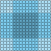
Figure 1. Covering of the domain by nine overlapping subdomains

Next, consider the partitioning (4.5) of the set $\mathcal{D}$ of DOF. We illustrate for the case of two grids, a coarse grid ${\mathcal{T}}_{H}$,and fine grid ${\mathcal{T}}_{h}$, where $H=2h$. Then the corresponding sets of edges are ${\mathcal{E}}_{H}$ and ${\mathcal{E}}_{h}$ with the following relations being obvious: $4|{\mathcal{T}}_{H}|=|{\mathcal{T}}_{h}|$ and $2|{\mathcal{E}}_{H}|+4|{\mathcal{T}}_{H}|=|{\mathcal{E}}_{h}|$. Since for lowest-order Raviart-Thomas finite elements it is not immediately clear how to partition $\mathcal{D}$, we perform a preprocessing step which consists of a compatible two-level basis transformation [14]. The global matrix $A$ is transformed according to

(4.25) $$\widehat{A}=J^{T}AJ,\quad\widehat{A},J,A\in\mathbb{R}^{|{\mathcal{E}}_{h}|\times|{\mathcal{E}}_{h}|},$$

where the transformation matrix $J$ is the product of a permutation matrix $P$ and another transformation matrix $J_{\pm}$, i.e.

(4.26) $$J=PJ_{\pm},\quad P,J_{\pm}\in\mathbb{R}^{|{\mathcal{E}}_{h}|\times|{\mathcal{E}}_{h}|}.$$

The permutation $P$ allows us to provide a two-level numbering of the DOF that splits them into two groups, the first one consisting of DOF associated with fine-grid edges not part of any coarse-grid edge (interior DOF) and the second keeping all remaining DOF ordered such that any two that are on one and the same coarse edge have consecutive numbers. The transformation matrix $J_{\pm}$ in (4.26) is of the form

$$J_{\pm}=\left[\begin{array}[]{cc}I&\\ &J_{22}\end{array}\right],\quad\mbox{where}\quad I\in\mathbb{R}^{(4|{\mathcal{T}_{H}}|)\times(4|{\mathcal{T}_{H}}|)},$$

and  $J_{22}=\frac{1}{2}\left[\begin{array}[]{cccccccc}1&-1&&&&&&\\ &&1&-1&&&&\\ &&&&\ddots&\ddots&&\\ &&&&&&-1&1\\ 1&1&&&&&&\\ &&1&1&&&&\\ &&&&\ddots&\ddots&&\\ &&&&&&1&1\end{array}\right],\quad\mbox{where}\ \ J_{22}\in\mathbb{R}^{(2|{\mathcal{E}_{H}}|)\times(2|{\mathcal{E}_{H}}|)}.$

The analogous transformation is performed at a local level on each subdomain $\Omega_{i}$, i.e.

(4.27) $$\widehat{A}_{i}=J^{T}_{i}A_{i}J_{i},$$

where again $J_{i}=P_{i}J_{\pm,i}$ with $P_{i}$ the permutation as explained above but performed on the degrees of freedom in the subdomain $\Omega_{i}$. $J_{\pm,i}$ has its usual meaning but restricted to the subdomain $\Omega_{i}$.

Definition 4.2.

Global and local transformations are called compatible if

$$\widehat{A}=J^{T}AJ=\sum_{i=1}^{n_{\mathcal{G}}}\widehat{R}_{i}^{T}\widehat{A}_{i}\widehat{R}_{i}$$

which is equivalent to the condition $R_{i}J=J_{i}\widehat{R}_{i}$ for all $i$.

The introduced transformation matrix $J$ defines the splitting of the DOF into coarse and fine, namely the FDOF correspond to the set of interior DOF and half differences on the coarse edges while the CDOF correspond to the half sums on the coarse edges.

This transformation can be applied recursively to coarse-level matrices. The corresponding two-level transformation matrices, referring to levels $k=0,1,\ldots,\ell-1$, are denoted by $J^{(k)}$.

Finally, the nonlinear ASMG preconditioner employs the following two-level matrices

$$\widehat{A}^{(k)}={J^{(k)}}^{T}A^{(k)}J^{(k)}$$

for all $k<\ell$. Its application to a vector $\widehat{{\bf{d}}}$ for the two-level basis at level $k$ can be formulated as follows.

Algorithm 4.1.

Action of preconditioner (4.20) on a vector $\widehat{{\bf{d}}}={J^{(k)}}^{T}{\bf{d}}$ at level $k$: $\widehat{C}^{(k)}[\widehat{{\bf{d}}}]$
  Auxiliary space correction: $\left\{\begin{array}[]{l}\left(\begin{array}[]{c}\tilde{{\bf{q}}}_{1}\\ \tilde{{\bf{q}}}_{2}\end{array}\right):=\tilde{{\bf{q}}}=\Pi_{\widetilde{D}^{(k)}}^{T}\widehat{{\bf{d}}}\\ \tilde{{\bf{p}}}_{1}=(\widetilde{A}^{(k)}_{11})^{-1}\tilde{{\bf{q}}}_{1}\\ \tilde{{\bf{p}}}_{2}={J^{(k+1)}}C_{{\rm GCG,\nu}}^{(k+1)}[{J^{(k+1)}}^{T}(\tilde{{\bf{q}}}_{2}-\widetilde{A}^{(k)}_{21}\tilde{{\bf{p}}}_{1})]\\ \tilde{{\bf{q}}}_{1}=\tilde{{\bf{p}}}_{1}-(\widetilde{A}^{(k)}_{11})^{-1}\widetilde{A}^{(k)}_{12}\tilde{{\bf{p}}}_{2}\\ \tilde{{\bf{q}}}_{2}=\tilde{{\bf{p}}}_{2}\\ \widehat{C}^{(k)}[\widehat{{\bf{d}}}]:=\Pi_{\widetilde{D}^{(k)}}\tilde{{\bf{q}}}\end{array}\right.$
 

By incorporating pre- and post-smoothing the realisation of the preconditioner (4.24) takes the following form.

Algorithm 4.2.

Action of preconditioner (4.24) on a vector $\widehat{{\bf{d}}}$ at level $k$: $\widehat{B}^{(k)}[\widehat{{\bf{d}}}]$
  Pre-smoothing: $\widehat{{\bf{u}}}=(\widehat{M}^{(k)})^{-1}\widehat{{\bf{d}}}$ Auxiliary space correction: $\widehat{{\bf{v}}}=\widehat{{\bf{u}}}+\widehat{C}^{(k)}[\widehat{{\bf{d}}}-\widehat{A}^{(k)}\widehat{{\bf{u}}}]$ Post-smoothing: $\widehat{B}^{(k)}[\widehat{{\bf{d}}}]:=\widehat{{\bf{v}}}+(\widehat{M}^{(k)})^{-T}(\widehat{{\bf{d}}}-\widehat{A}^{(k)}\widehat{{\bf{v}}})$
 

4.4. On the complexity of the ASMG preconditioner

We now address the important topic of estimating the computational work required for performing the action of the ASMG preconditioner. Clearly, from the algorithm descriptions given earlier, the number of flops required to evaluate such an action is proportional to the operator complexity of the preconditioner, defined as the total number of non-zeroes in the matrices on all levels. The most general algebraic multilevel preconditioners are usually constructed using the combinatorial graph structure of the underlying matrices (on the finest and coarser levels). Estimating the operator complexities in such cases is not only difficult, but in most cases impossible due to the fact that such estimates should hold for the set of all possible graphs. Reliable estimates are usually done for algorithms that construct coarse levels using at least some of the geometric information from the underlying problem. This is the case we consider here, and we also refer to [5], [31] for more insight into how geometric information can be used to bound the operator complexity of a multilevel preconditioner.

Given a matrix $A\in\mathbb{R}^{N\times N}$, we characterize the nonzero structure of the ASMG coarse level matrix $Q$. To construct $Q$, recall that we first need to split the set of the degrees of freedom as a union of subsets, $\{1,\ldots,N\}=\cup_{i=1}^{n}\omega_{i}$. We assume that $\omega_{i}=\{\mathcal{F}_{i},\mathcal{C}_{i}\}$, where $\mathcal{F}_{i}$ is a set of fine grid degrees of freedom, and, $\mathcal{C}_{i}$, is a set of coarse grid degrees of freedom, with $\mathcal{F}_{i}\cap\mathcal{C}_{i}=\emptyset$. The total number of coarse grid degrees of freedom is $N_{\mathcal{C}}=\left|\cup_{j=1}^{n}\mathcal{C}_{i}\right|$. Since our considerations are permutation invariant, without loss of generality, we assume that globally we have numbered first the coarse grid degrees of freedom, and thus we have $\mathcal{C}_{i}\subset\{1,\ldots,N_{\mathcal{C}}\}$.

We also set $N_{i}=|\omega_{i}|$, and $n_{i}=|\mathcal{C}_{i}|$. We denote by ${\bf e}_{k}$ the $k$-th Euclidean basis vector in $\mathbb{R}^{N}$; when we consider the canonical basis in $\mathbb{R}^{m}$, $m\neq N$, we use the notation ${\bf e}_{k(m)}$ for the $k$-th basis vector. With each $\omega_{i}$ we associate a matrix $R_{i}\in\mathbb{R}^{N_{i}\times N}$, and, for $\omega_{i}=\{j_{1},\ldots,j_{N_{i}}\}$, we set $R^{T}_{i}=[{\bf e}_{j_{1}},\ldots,{\bf e}_{j_{N_{i}}}]$. Next, we consider a fine grid matrix $A$ given by the identity

$$A=\sum_{i=1}^{n}R^{T}_{i}A_{i}R_{i}=\sum_{i=1}^{n}\begin{bmatrix}R^{T}_{i,\mathcal{F}},R^{T}_{i,\mathcal{C}}\end{bmatrix}\begin{bmatrix}A_{i,\mathcal{F}}&A_{i,\mathcal{FC}}\\ A_{i,\mathcal{CF}}&A_{i,\mathcal{C}}\end{bmatrix}\begin{bmatrix}R_{i,\mathcal{F}}\\ R_{i,\mathcal{C}}\end{bmatrix}$$

where we used a block form of the matrices corresponding to the splitting of $\omega_{i}$ on $\mathcal{F}$-ine level and $\mathcal{C}$-oarse level degrees of freedom. The Schur complements $S_{i}$ used in the definition of the coarse grid matrix $Q$ are defined as $S_{i}=A_{i,\mathcal{C}}-A_{i,\mathcal{CF}}A_{i,\mathcal{F}}^{-1}A_{i,\mathcal{FC}}$. Recall that the coarse grid matrix $Q$ then is defined by $Q=\sum_{i=1}^{n}\widetilde{R}^{T}_{i,\mathcal{C}}S_{i}\widetilde{R}_{i,\mathcal{C}},\quad\mbox{and we have}\quad Q\in\mathbb{R}^{N_{\mathcal{C}}\times N_{\mathcal{C}}}.$ If we now use our assumption that the coarse grid degrees of freedom are numbered first, then $\widetilde{R}_{i,\mathcal{C}}\in\mathbb{R}^{n_{i}\times N_{\mathcal{C}}}$ is formed by the first $N_{\mathcal{C}}$ columns of $R_{i,\mathcal{C}}\in\mathbb{R}^{n_{i}\times N_{\mathcal{C}}}$. Next, we introduce the vectors $\bm{1}_{i}=(\underbrace{1,\ldots,1}_{n_{i}})^{T}$, and $\bm{\chi}_{i}=\sum_{j\in\mathcal{C}_{i}}{\bf e}_{j(N_{\mathcal{C}})}$. For a fixed $i$, the vector $\bm{\chi}_{i}\in\mathbb{R}^{N}$ is the indicator vector of the set $\mathcal{C}_{i}$ as a subset of $\{1,\ldots,N_{\mathcal{C}}\}$. Its components are equal to $1$ for indicies in $\mathcal{C}_{i}$ and equal to zero otherwise. We note that $\bm{1}_{i}\bm{1}_{i}^{T}$ is the $n_{i}\times n_{i}$ matrix of all ones, and we encourage the reader to check the identity $\bm{\chi}_{i}=\widetilde{R}_{i,\mathcal{C}}^{T}\bm{1}_{i}$.

To describe the nonzero structure of $Q$ we introduce the set $\mathcal{B}_{m}$ of Boolean $(m\times m)$ matrices whose entries are from the set $\{0,1\}$. We introduce a mapping $\operatorname{nz}:\mathbb{R}^{m\times m}\mapsto\mathcal{B}_{m}$, such that $[\operatorname{nz}(A)]_{ij}=0$ if and only if $A_{ij}=0$ and $[\operatorname{nz}(A)]_{ij}=1$ otherwise. We say that $X\preceq Y$ if $[\operatorname{nz}(Y)-\operatorname{nz}(X)]$ is a matrix with non-negative entries. This is a formal way to state that the nonzero structure of $Y$ contains the nonzero structure of $X$, or, to say that every zero in $Y$ is also a zero in $X$. Clearly, $S_{i}\preceq\bm{1}_{i}\bm{1}_{i}^{T}$, and, as a consequence, we have the following relation characterizing the sparsity of $Q$:

(4.28) $$Q\preceq\sum_{i=1}^{n}\sum_{i=1}^{n}\widetilde{R}_{i,\mathcal{C}}^{T}\bm{1}_{i}\bm{1}_{i}^{T}\widetilde{R}_{i,\mathcal{C}}=\sum_{i=1}^{n}\bm{\chi}_{i}\bm{\chi}_{i}^{T}=:X.$$

Note that from the right side of (4.28) we can conclude that $Q_{km}$ may be nonzero only in the case when there exists $i$ such that $k\in\mathcal{C}_{i}$ and $m\in\mathcal{C}_{i}$. Using (4.28) it is easy to compute a bound on the number of non-zeroes $n_{z,j}$, for fixed column $j$ in $Q$. We have

$$n_{z,j}\leq\|X{\bf e}_{j(N_{\mathcal{C}})}\|_{\ell^{1}}=\sum_{i:j\in\mathcal{C}_{i}}|\mathcal{C}_{i}|.$$

As is immediately seen, the number of non-zeroes per column in $Q$ is bounded by a constant independent of $N$ if the following two conditions are satisfied: (i) the number of coarse grid degrees of freedom in each $\mathcal{C}_{i}$ is bounded; and (ii) every coarse grid degree of freedom lies in a bounded number of subsets $\mathcal{C}_{i}$.

As a simple, but instructive example how the conditions (i) and (ii) can be satisfied, let us consider a PDE discretized by FE method on a quasiuniform grid with characteristic mesh size $h$ in 2D. The considerations are independent of the PDE or the order of the FE spaces (but the constants hidden in “$\lesssim$” below may depend on the FE spaces and the order of polynomials). To define the sets $\omega_{i}$ on such a grid, we proceed as follows: (1) place a regular (square) auxiliary grid of size $\gamma h$, $\gamma\geq 2$ that contains $\Omega$; (2) set $n$ to be the number of vertices on the auxiliary grid, lying in $\Omega$; (3) choose $\omega_{i}$ to be the set of DOF degrees of freedom lying in the support of the bilinear basis function corresponding to the $i$-th vertex. Then we have that $|\mathcal{C}_{i}|<N_{i}\lesssim 4\gamma$ and every coarse grid degree of freedom lies in at most $4$ such subdomains. The constant hidden in “$\lesssim$” is a bound on the number of degrees of freedom lying in a square of size $2h$. The fact that this bound depends only on the polynomial order and type of FE spaces follows from the assumption that the mesh is quasi-uniform. For efficient and more sophisticated techniques using regular, but adaptively refined, auxiliary grids in coarsening algorithms for unstructured problems we refer to [5], [31]. Such techniques may directly be applied to yield optimal operator complexities for the ASMG preconditioner in the general case of shape regular grids, albeit the details are beyond the scope of our consideration here.

5. Numerical Experiments

5.1. Description of the parameters and the numerical test examples

Subject to numerical testing are three representative cases characterised by a highly varying coefficient ${\alpha}(x)=K^{-1}(x)$, namely:

1. ] A binary distribution of the coefficient described by islands on which ${\alpha}=1.0$ against a background where ${\alpha}=10^{-q}$, see Figure 2;

2. ] Inclusions with ${\alpha}=1.0$ and a background with a coefficient ${\alpha}={\alpha}_{T}=10^{-q_{rand}}$ that is constant on each element $\tau\in{\mathcal{T}}_{h}$, where the random integer exponent $q_{rand}\in\{0,1,2,\dots,q\}$ is uniformly distributed, see Figure 3;

3. ] Three two-dimensional slices of the SPE10 benchmark problem, where the contrast $\kappa$ is $10^{7}$ for slices 44 and 74 and $10^{6}$ for slice 54, see Figure 4.

Test problems [a] and [b] are similar to those considered in other works, e.g. [8, 15, 32]. Example [c] consists of 2-D slices of 3-dimensional data of SPE10 (Society of Petroleum Engineers) benchmark, see [12].

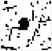
(a) $32\times 32$ mesh

(b) $128\times 128$ mesh

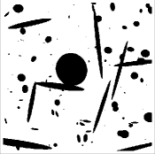
(c) $512\times 512$ mesh

Figure 2. Binary distribution of the permeability $K(x)$ corresponding to test case [a]

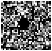
(a) $32\times 32$ mesh

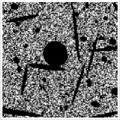
(b) $128\times 128$ mesh

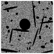
(c) $512\times 512$ mesh

Figure 3. Random distribution of ${\alpha}=K^{-1}(x)$ corresponding to test case [b]

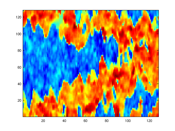
(a) Slice 44

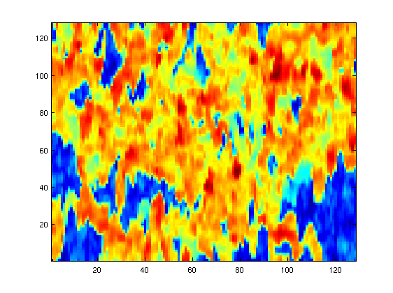
(b) Slice 54

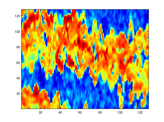
(c) Slice 74

Figure 4. Distributions of the permeability $K(x)$ along planes $x_{3}=44,54,74$ from the benchmark SPE10 on a $128\times 128$ mesh

The numerical experiments were performed over a uniform mesh consisting of $N{\times}N$ square elements where $N=4,8,\ldots,512$, i.e. up to $525312$ velocity DOF and $262144$ pressure DOF. We have used a direct method to solve the problems on the coarsest grid. The iterative process has been initialised with a random vector. Its convergence has been tested for linear systems with the right hand side zero except in the last example where we have solved the mixed system (1.1) for slice 44 of the SPE10 problem with the right hand side

(5.1) $$f=\left\{\begin{array}[]{rcl}c&\mbox{for}&(x,y)\in\Omega_{+}=[0.2,0.3]{\times}[0.7,0.8]\\ -c&\mbox{for}&(x,y)\in\Omega_{-}=[0.7,0.8]{\times}[0.2,0.3]\\ 0&\mbox{for}&(x,y)\in\Omega\setminus(\Omega_{+}\cup\Omega_{-})\end{array}\right.$$

We have used overlapping coverings of the domain as shown in Figure 1, where the subdomains are composed of $8\times 8$ elements and overlap with half their width or height. When presenting results we use the following notation:

• $\ell$ denotes the number of levels;

• $q=\frac{\log\kappa}{\log 10}$ is the logarithm of the contrast $\kappa$;

• $n_{ASMG}$ is the number of auxiliary space multigrid iterations;

• $m\geq 0$ is the number of point Gauss-Seidel pre- and post-smoothing steps;

• $\rho_{r}$ is the average residual reduction factor defined by

  (5.2) $$\rho_{r}=\Bigg{(}\frac{\|{\bf{r}}_{n_{ASMG}}\|}{\|{\bf{r}}_{0}\|}\Bigg{)}^{1/n_{ASMG}},$$

  where ${\bf{u}}_{n_{ASMG}}$ is the first iterate (approximate solution of (4.4)) for which the initial residual has decreased by a factor of at least $10^{8}$;

• $\rho_{e}:=\|I-{{C}^{(0)}}^{-1}A^{(0)}\|_{A^{(0)}}$ is the norm of the error propagation matrix of the linear V-cycle preconditioner (4.20) which is obtained by choosing the polynomial $p_{\nu}(t)=1-t$ in (4.22).

The matrix $\widetilde{D}$ is as in (4.12) where $\widetilde{D}_{11}=\widetilde{A}_{11}$. This choice of $\widetilde{D}$ requires an additional preconditioner for the iterative solution of linear systems with the matrix $D=R\widetilde{D}R^{T}$ a part of the efficient application of the operator $\Pi_{\widetilde{D}}$. The systems with $D$ are solved using the preconditioned conjugate gradient (PCG) method. The stopping criterion for this inner iterative process is a residual reduction by a factor $10^{6}$, the number of PCG iterations to reach it–where reported–is denoted by $n_{i}$. The preconditioner $B_{ILUE}$ for $D$ is constructed using incomplete factorisation with exact local factorisation (ILUE). The definition of $B_{ILUE}$ is as follows:

$$B_{ILUE}:=LU,\qquad U:=\sum_{i=1}^{n}R_{i}^{T}U_{i}R_{i},\qquad L:=U^{T}{\rm diag}(U)^{-1},$$

where

$$D_{i}=L_{i}U_{i},\qquad D=\sum_{i=1}^{n}R_{i}^{T}D_{i}R_{i},\qquad{\rm diag}(L_{i})=I.$$

For details see [16]. Note that as $D_{i}$ are the local contributions to $D$ related to the subdomains $\Omega_{i}$, $i=1,\dots,n$, they are all non-singular.

The following two sections are devoted to the presentation of numerical results. Experiments fall into two categories. The first category, presented in Section 5.2, serves the evaluation of the performance of the ASMG method on linear systems arising from discretisation of the weighted ${\bm{H}}(\operatorname{div})$ bilinear form (2.5). All three test cases, [a], [b], and [c], are considered testing V- and W-cycle methods with and without smoothing. Additionally, we evaluate as a robustness indicator the quantity $\|\pi_{\widetilde{D}}\|^{2}_{\widetilde{A}}=\|R^{T}\Pi_{\widetilde{D}}\|^{2}_{\widetilde{A}}$, which appears in (4.14) and (4.15).

The second category of experiments, discussed in Section 5.3, addresses the solution of the indefinite linear system (1.2) arising from problem (2.10) by a preconditioned MinRes method. The main aims are, on the one hand, to confirm the robustness of the block-diagonal preconditioner (4.3) with respect to arbitrary multiscale coefficient variations, and on the other, to demonstrate its numerical scalability. Furthermore, we include a test problem with a nonzero right hand side.

5.2. Numerical tests for solving the system (4.4)

An ASMG preconditioner was tested for solving the system (4.4) with a matrix corresponding to discretisation of the form $\Lambda_{\alpha}({\mathbf{u}},{\mathbf{v}})$.

Example 5.1.

First we estimate $\|\pi_{\widetilde{D}}\|^{2}_{\widetilde{A}}$ at the level of the finest mesh, level $0$, for increasing contrast of magnitude $10^{q}$ in the configuration of case [b].

The experimental study is based on Lemma 4.1. The quantity of interest in Example 5.1 provides an upper bound for the condition number $\kappa(C^{-1}A)$ for the two-level preconditioner (4.13). The results shown in Table 2 clearly demonstrate that $\kappa(C^{-1}A)$ is uniformly bounded.

This test indicates the robustness of the fictitious space preconditioner with respect to a highly varying coefficient on multiple length scales. Note that test case [b] is considered to be representative, taking into account the iteration counts for the test cases [a] and [b] as presented in the following examples.

Value of $\|\pi_{\widetilde{D}}\|^{2}_{\widetilde{A}}$: bilinear form (2.5)
	$\ell=3$	$\ell=4$	$\ell=5$	$\ell=6$	$\ell=7$
$q=0$	$1.122$	$1.137$	$1.148$	$1.150$	$1.149$
$q=1$	$1.148$	$1.169$	$1.149$	$1.152$	$1.138$
$q=2$	$1.286$	$1.338$	$1.360$	$1.287$	$1.126$
$q=3$	$1.336$	$1.389$	$1.418$	$1.326$	$1.132$
$q=4$	$1.343$	$1.396$	$1.426$	$1.334$	$1.133$
$q=5$	$1.343$	$1.397$	$1.426$	$1.333$	$1.369$
$q=6$	$1.343$	$1.397$	$1.426$	$1.333$	$1.369$

Table 1. Example 5.1: case [a] with $K(x)=10^{q}$

Value of $\|\pi_{\widetilde{D}}\|^{2}_{\widetilde{A}}$: bilinear form (2.5)
	$\ell=3$	$\ell=4$	$\ell=5$	$\ell=6$	$\ell=7$
$q=0$	$1.122$	$1.137$	$1.148$	$1.150$	$1.149$
$q=1$	$1.115$	$1.126$	$1.169$	$1.167$	$1.123$
$q=2$	$1.126$	$1.208$	$1.119$	$1.146$	$1.112$
$q=3$	$1.014$	$1.261$	$1.338$	$1.334$	$1.110$
$q=4$	$1.260$	$1.295$	$1.371$	$1.434$	$1.110$
$q=5$	$1.268$	$1.329$	$1.394$	$1.493$	$1.145$
$q=6$	$1.255$	$1.374$	$1.412$	$1.139$	$1.113$

Table 2. Example 5.1: case [b] with $K(x)=10^{q}$

Example 5.2.

Next we are interested in the convergence factor in $A$-norm of the linear V-cycle method, that is, we evaluate the quantity $\rho_{e}:=\|I-{{C}^{(0)}}^{-1}A^{(0)}\|_{A^{(0)}}$. Moreover, we compare $\rho_{e}$ to the corresponding value of the average residual reduction factor $\rho_{r}$ defined according to (5.2). We also report the number of iterations $it_{e}$ that reduce the initial error in $A$-norm by a factor $10^{8}$ and the number of iterations $it_{r}$ that reduce the Euclidean norm of the initial residual by the same factor. The problem configuration is test case [c] for a zero right hand side.

The results for Example 5.2 are summarised in Table 3. Although the average residual reduction factor $\rho_{r}$ is much smaller than $\rho_{e}$, the error reduction in the $A$-norm is also surprisingly good, especially in view of the linear V-cycle performing without any additional smoothing, i.e., implementing Algorithm 4.1.

Linear V-cycle: bilinear form (2.5)
	$\rho_{e}$	$it_{e}$	$\rho_{r}$	$it_{r}$
$\ell=4$	$0.105$	$7$	$0.031$	$6$
$\ell=5$	$0.289$	$9$	$0.095$	$8$
$\ell=6$	$0.494$	$12$	$0.168$	$11$
$\ell=7$	$~{}~{}0.642~{}~{}$	$~{}~{}~{}14~{}~{}~{}$	$~{}~{}0.215~{}~{}$	$~{}~{}~{}12~{}~{}~{}$
$\ell=8$	$0.729$	$17$	$0.262$	$14$

Table 3. Example 5.2: case [c] - slice 44 of the SPE10 benchmark.

Example 5.3.

Now we test the nonlinear V-cycle and the effect of additional smoothing. Again the problem configuration is test case [c] for a zero right hand side. We report the number of nonlinear AMLI-cycle ASMG iterations with Algorithm 4.1 denoted by $n_{ASMG}$ for a residual reduction by eight orders of magnitude along with $\rho_{r}$.

Comparing the results for Example 5.3, which are listed in Table 4, with those in Table 3 shows that the nonlinear V-cycle typically also reduces the residual norm faster than the linear V-cycle–for the reduction of the $A$-norm of the error this is a known fact–and the additional incorporation of a point Gauss-Seidel relaxation further accelerates the convergence.

Non-linear V-cycle: bilinear form (2.5)
	$m=0$		$m=1$		$m=2$
	$n_{ASMG}$	$\rho$	$n_{ASMG}$	$\rho$	$n_{ASMG}$	$\rho$
$\ell=4$	$6$	$0.032$	$5$	$0.025$	$6$	$0.027$
$\ell=5$	$8$	$0.093$	$7$	$0.062$	$6$	$0.045$
$\ell=6$	$11$	$0.157$	$8$	$0.091$	$8$	$0.083$
$\ell=7$	$12$	$0.202$	$9$	$0.123$	$8$	$0.094$
$\ell=8$	$14$	$0.243$	$11$	$0.172$	$10$	$0.154$

Table 4. Example 5.3: case [c] - slice 44 of the SPE10 benchmark.

Example 5.4.

The next example tests the dependency of the convergence rate with respect to the contrast. The configuration is test case [a] containing a zero right hand side and number of smoothing steps $m=2$.

Results in Table 5 show a slight increase in $\rho_{r}$ with increasing contrast.

ASMG V-cycle: bilinear form (2.5), Algorithm 4.1
	$\ell=3$		$\ell=4$		$\ell=5$		$\ell=6$		$\ell=7$
	$n_{ASMG}$	$\rho$	$n_{ASMG}$	$\rho$	$n_{ASMG}$	$\rho$	$n_{ASMG}$	$\rho$	$n_{ASMG}$	$\rho$
$q=0$	$4$	$0.005$	$5$	$0.024$	$6$	$0.043$	$8$	$0.083$	$8$	$0.093$
$q=1$	$3$	$0.002$	$5$	$0.022$	$7$	$0.058$	$8$	$0.084$	$9$	$0.121$
$q=2$	$3$	$0.002$	$5$	$0.019$	$7$	$0.068$	$8$	$0.091$	$9$	$0.121$
$q=3$	$3$	$0.002$	$5$	$0.018$	$7$	$0.070$	$8$	$0.095$	$9$	$0.125$
$q=4$	$3$	$0.002$	$5$	$0.017$	$7$	$0.069$	$8$	$0.098$	$10$	$0.142$
$q=5$	$3$	$0.002$	$5$	$0.017$	$8$	$0.082$	$9$	$0.118$	$10$	$0.145$
$q=6$	$4$	$0.005$	$4$	$0.010$	$8$	$0.092$	$9$	$0.125$	$11$	$0.181$

Table 5. Example 5.4: case [a] with $K(x)=10^{q}$ and two smoothing steps ($m=2$).

Example 5.5.

In the next set of numerical experiments we consider the same distribution of inclusions of low permeability as before but this time against the background of a randomly distributed piecewise constant permeability coefficient as shown in Figure 3.

The results, presented in Tables 6 and 7, are even better than those obtained for the binary distribution in the sense that both the $V$- and $W$-cycle are robust with respect to the contrast.

ASMG V-cycle: bilinear form (2.5), Algorithm 4.1
	$\ell=3$		$\ell=4$		$\ell=5$		$\ell=6$		$\ell=7$
	$n_{ASMG}$	$\rho$	$n_{ASMG}$	$\rho$	$n_{ASMG}$	$\rho$	$n_{ASMG}$	$\rho$	$n_{ASMG}$	$\rho$
$q=0$	$4$	$0.007$	$6$	$0.027$	$9$	$0.102$	$10$	$0.156$	$12$	$0.210$
$q=1$	$4$	$0.006$	$6$	$0.035$	$9$	$0.103$	$11$	$0.171$	$13$	$0.224$
$q=2$	$4$	$0.005$	$6$	$0.032$	$9$	$0.102$	$11$	$0.159$	$13$	$0.222$
$q=3$	$4$	$0.006$	$6$	$0.042$	$9$	$0.110$	$11$	$0.174$	$13$	$0.229$
$q=4$	$4$	$0.006$	$7$	$0.043$	$9$	$0.127$	$11$	$0.183$	$13$	$0.233$
$q=5$	$4$	$0.006$	$7$	$0.049$	$10$	$0.138$	$12$	$0.195$	$13$	$0.239$
$q=6$	$4$	$0.006$	$7$	$0.056$	$10$	$0.149$	$12$	$0.207$	$14$	$0.252$

Table 6. Example 5.5: case [b], no smoothing steps ($m=0$).

ASMG V-cycle: bilinear form (2.5), Algorithm 4.1
	$\ell=3$		$\ell=4$		$\ell=5$		$\ell=6$		$\ell=7$
	$n_{ASMG}$	$\rho$	$n_{ASMG}$	$\rho$	$n_{ASMG}$	$\rho$	$n_{ASMG}$	$\rho$	$n_{ASMG}$	$\rho$
$q=0$	$4$	$0.005$	$5$	$0.024$	$6$	$0.046$	$8$	$0.083$	$8$	$0.091$
$q=1$	$4$	$0.005$	$6$	$0.033$	$7$	$0.060$	$8$	$0.091$	$9$	$0.124$
$q=2$	$3$	$0.002$	$5$	$0.023$	$6$	$0.045$	$7$	$0.069$	$9$	$0.121$
$q=3$	$3$	$0.002$	$5$	$0.021$	$6$	$0.043$	$7$	$0.071$	$8$	$0.100$
$q=4$	$4$	$0.005$	$5$	$0.023$	$6$	$0.044$	$8$	$0.089$	$9$	$0.122$
$q=5$	$4$	$0.005$	$5$	$0.024$	$6$	$0.045$	$8$	$0.090$	$9$	$0.125$
$q=6$	$4$	$0.005$	$6$	$0.034$	$6$	$0.045$	$8$	$0.091$	$10$	$0.142$

Table 7. Example 5.5: case [b] with two smoothing steps ($m=2$).

ASMG W-cycle: bilinear form (2.5), Algorithm 4.1
	$\ell=3$		$\ell=4$		$\ell=5$		$\ell=6$		$\ell=7$
	$n_{ASMG}$	$\rho$	$n_{ASMG}$	$\rho$	$n_{ASMG}$	$\rho$	$n_{ASMG}$	$\rho$	$n_{ASMG}$	$\rho$
$q=0$	$4$	$0.005$	$4$	$0.007$	$4$	$0.006$	$4$	$0.005$	$4$	$0.005$
$q=1$	$4$	$0.006$	$4$	$0.007$	$4$	$0.007$	$4$	$0.006$	$4$	$0.005$
$q=2$	$4$	$0.004$	$4$	$0.009$	$5$	$0.016$	$4$	$0.007$	$4$	$0.006$
$q=3$	$4$	$0.005$	$5$	$0.015$	$5$	$0.015$	$4$	$0.009$	$4$	$0.006$
$q=4$	$4$	$0.005$	$5$	$0.016$	$5$	$0.016$	$4$	$0.009$	$4$	$0.008$
$q=5$	$4$	$0.005$	$5$	$0.018$	$5$	$0.015$	$4$	$0.009$	$4$	$0.008$
$q=6$	$4$	$0.005$	$5$	$0.019$	$5$	$0.015$	$4$	$0.008$	$4$	$0.007$

Table 8. Example 5.5: case [b] with one smoothing step ($m=1$).

Example 5.6.

The last set of experiments in the first category is devoted to test case [c] where, similarly to Example 5.2, we examine the performance of the preconditioner for a bilinear form (2.5). Here, we compare the ASMG preconditioners for three different coefficient distributions, namely slices 44, 54, and 74 of the SPE10 benchmark problem. In this example the finest mesh is always composed of $256\times 256$ elements, meaning that changing the number of levels $\ell$ refers to a different size of the coarse-grid problem.

Tables 9–11 report the number of outer iterations $n_{ASMG}$ and the maximum number of inner iterations $n_{i}$ needed to reduce the residual with the matrix $R\widetilde{D}R^{T}$ by a factor of $10^{6}$.

ASMG V-cycle and W-cycle: bilinear form (2.5)
	V-cycle						W-cycle
	$m=0$			$m=1$			$m=0$			$m=1$
	$n_{ASMG}$	$\rho$	$n_{i}$	$n_{ASMG}$	$\rho$	$n_{i}$	$n_{ASMG}$	$\rho$	$n_{i}$	$n_{ASMG}$	$\rho$	$n_{i}$
$\ell=3$	$8$	$0.080$	$4$	$7$	$0.064$	$5$	$5$	$0.019$	$6$	$5$	$0.014$	$5$
$\ell=4$	$10$	$0.157$	$6$	$9$	$0.122$	$6$	$5$	$0.019$	$6$	$5$	$0.014$	$5$
$\ell=5$	$12$	$0.209$	$6$	$10$	$0.154$	$6$	$5$	$0.019$	$6$	$5$	$0.014$	$5$
$\ell=6$	$13$	$0.239$	$6$	$11$	$0.179$	$6$	$5$	$0.019$	$6$	$5$	$0.014$	$5$
$\ell=7$	$13$	$0.239$	$6$	$11$	$0.179$	$6$	$5$	$0.019$	$6$	$5$	$0.014$	$5$

Table 9. Example 5.6: case [c] - slice 44 of the SPE10 benchmark.

ASMG V-cycle and W-cycle: bilinear form (2.5)
	V-cycle						W-cycle
	$m=0$			$m=1$			$m=0$			$m=1$
	$n_{ASMG}$	$\rho$	$n_{i}$	$n_{ASMG}$	$\rho$	$n_{i}$	$n_{ASMG}$	$\rho$	$n_{i}$	$n_{ASMG}$	$\rho$	$n_{i}$
$\ell=3$	$7$	$0.070$	$4$	$7$	$0.059$	$4$	$5$	$0.016$	$4$	$5$	$0.013$	$4$
$\ell=4$	$10$	$0.156$	$5$	$9$	$0.122$	$6$	$5$	$0.017$	$6$	$5$	$0.013$	$5$
$\ell=5$	$13$	$0.236$	$5$	$11$	$0.173$	$6$	$5$	$0.018$	$6$	$5$	$0.013$	$6$
$\ell=6$	$14$	$0.253$	$5$	$11$	$0.183$	$6$	$5$	$0.018$	$6$	$5$	$0.013$	$6$
$\ell=7$	$14$	$0.253$	$6$	$11$	$0.183$	$6$	$5$	$0.018$	$6$	$5$	$0.013$	$6$

Table 10. Example 5.6: case [c] - slice 54 of the SPE10 benchmark.

ASMG V-cycle and W-cycle: bilinear form (2.5)
	V-cycle						W-cycle
	$m=0$			$m=1$			$m=0$			$m=1$
	$n_{ASMG}$	$\rho$	$n_{i}$	$n_{ASMG}$	$\rho$	$n_{i}$	$n_{ASMG}$	$\rho$	$n_{i}$	$n_{ASMG}$	$\rho$	$n_{i}$
$\ell=3$	$8$	$0.090$	$4$	$7$	$0.070$	$4$	$5$	$0.019$	$4$	$5$	$0.014$	$4$
$\ell=4$	$11$	$0.178$	$5$	$10$	$0.145$	$5$	$5$	$0.020$	$5$	$5$	$0.015$	$5$
$\ell=5$	$13$	$0.229$	$5$	$11$	$0.166$	$6$	$5$	$0.020$	$6$	$5$	$0.015$	$6$
$\ell=6$	$13$	$0.242$	$6$	$11$	$0.180$	$6$	$5$	$0.020$	$6$	$5$	$0.015$	$6$
$\ell=7$	$13$	$0.242$	$6$	$11$	$0.180$	$6$	$5$	$0.020$	$6$	$5$	$0.015$	$6$

Table 11. Example 5.6: case [c] - slice 74 of the SPE10 benchmark.

5.3. Testing of block-diagonal preconditioner for system (1.2) within MinRes iteration

Now we present a number of numerical experiments for solving the mixed finite element system (1.2) with a preconditioned MinRes method. We consider two different examples, firstly, Example 5.7 in which the performance of the block-diagonal preconditioner and its dependence on the accuracy of the inner solves with W-cycle ASMG preconditioner is evaluated, and secondly, Example 5.8. testing the scalability of the MinRes iteration, again using a W-cycle ASMG preconditioner with one smoothing step for the inner iterations.

Example 5.7.

Here we apply the MinRes iteration to solve (1.2) for test case [c]. The hierarchy of meshes is the same as in Example 5.3. An ASMG W-cycle based on Algorithm 4.1 with one smoothing step has been used as a preconditioner on the ${\mathcal{RT}}_{0}$ space. Table 12 shows the number of MinRes iterations denoted by $n_{MinRes}$, the maximum number of ASMG iterations $n_{ASMG}$ needed to achieve an ASMG residual reduction by $\varpi$.

MinRes iteration: saddle point system (1.2)
	$\varpi=10^{6}$		$\varpi=10^{8}$		$\varpi=10^{10}$
	$n_{MinRes}$	$n_{ASMG}$	$n_{MinRes}$	$n_{ASMG}$	$n_{MinRes}$	$n_{ASMG}$
$\ell=3$	$24$	$4$	$17$	$6$	$15$	$8$
$\ell=4$	$15$	$5$	$13$	$6$	$13$	$8$
$\ell=5$	$21$	$5$	$17$	$6$	$15$	$8$
$\ell=6$	$22$	$5$	$17$	$6$	$15$	$8$
$\ell=7$	$22$	$5$	$17$	$6$	$15$	$8$

Table 12. Example 5.7: case [c] - slice 44 of the SPE10 benchmark. The hierarchy of meshes is the same as in Example 5.6.

Example 5.8.

In this set of experiments the MinRes iteration has been used to solve (1.2) for test case [c] for the same hierarchy of meshes as in Example 5.2. An ASMG W-cycle based on Algorithm 4.1 with one smoothing step has been used as a preconditioner on the ${\mathcal{RT}}_{0}$ space for a residual reduction by $10^{8}$. Table 13 shows the number of MinRes iterations $n_{MinRes}$, the maximum number of inner ASMG iterations $n_{ASMG}$ per outer MinRes iteration, and the number of DOF. Note that so long as the product $n_{MinRes}n_{ASMG}$ is constant, the total number of arithmetic operations required to achieve any prescribed accuracy is proportional to the number of DOF.

MinRes iteration: saddle point system (1.2)
			zero r.h.s.		nonzero r.h.s.
	DOF	$n_{MinRes}$	$n_{ASMG}$	$n_{MinRes}$	$n_{ASMG}$
$\ell=4$	$3,136$	$13$	$5$	$13$	$5$
$\ell=5$	$12,416$	$13$	$6$	$14$	$6$
$\ell=6$	$49,408$	$15$	$6$	$17$	$6$
$\ell=7$	$197,120$	$17$	$6$	$17$	$6$
$\ell=8$	$787,456$	$17$	$6$	$18$	$6$

Table 13. Example 5.8: case [c] - slice 44 of the SPE10 benchmark.

5.4. Comments regarding the numerical experiments and some general conclusions

The presented numerical results clearly demonstrate the efficiency of the proposed algebraic multilevel iteration (AMLI)-cycle auxiliary space multigrid (ASMG) preconditioner for problems with highly varying coefficients as they typically arise in the mathematical modelling of physical processes in high-contrast and high-frequency media.

During the first tests we evaluated the quantity $\|\pi_{\widetilde{D}}\|^{2}_{\widetilde{A}}$, which by Lemma 4.1 provides an upper bound for the condition number $\kappa(C^{-1}A)$. Then the convergence factor in A-norm of the linear V-cycle method was numerically studied. The above reported results show robustness with respect to a highly varying coefficient on multiple length scales. They also confirm that the nonlinear V-cycle reduces the residual norm faster than the linear V-cycle.

The next group of tests examines the convergence behaviour of the nonlinear ASMG method for the weighted bilinear form (2.5). This is a key point in the presented study. Cases [a] and [b] are designed to represent a typical multiscale geometry with islands and channels. Although case [b], a background with a random coefficient, appears to be more complicated, the impact of the multiscale heterogeneity seems to be stronger in binary case [a] where the number of iterations is slightly larger. However, in both cases we observe a uniformly converging ASMG V-cycle with $m=2$ and W-cycle ($\nu=2$) with $m=1$. Case [c] (SPE10) is a benchmark problem in the petroleum engineering community. Here we observe robust and uniform convergence with respect to the number of levels $\ell$, or, equivalently, mesh-size $h$. Note that such uniform convergence is recorded for the ASMG V-cycle even without smoothing iterations (i.e. $m=0$).

The results presented in Table 12–13, confirm the expected optimal convergence rate of the block-diagonally preconditioned MinRes iteration applied to the coupled saddle point system (1.2). Results in Table 12 demonstrate how the efficiency (in terms of the product $n_{MinRes}n_{ASMG}$) is achieved for a relative accuracy of $10^{-8}$ of the inner ASMG solver. Table 13 illustrates the scalability of the solver indicated by an almost constant number of MinRes and ASMG iterations since the total computational work in terms of fine grid matrix vector multiplications is proportional to the product $n_{MinRes}n_{ASMG}$. The case of a non-homogeneous right hand side provides a promising indicator for robustness of the ASMG preconditioner beyond the frame of the presented theoretical analysis.

Although not in the scope of this study, we note that the proposed auxiliary space multigrid method would be suitable for implementation on distributed memory computer architectures.

References

- [1] D. Arnold, R. Falk, and R. Winther. Preconditioning in H(div) and applications. Mathematics of Computation, 66:957–984, 1997.
- [2] D. Arnold, R. Falk, and R. Winther. Multigrid in H(div) and H(curl). Numer. Math., 85(2):197–217, 2000.
- [3] D. Börm and R. Hiptmair. Analysis of tensor multigrid. Numer. Algorithms, 26:219–234, 2001.
- [4] J. Bramble and X. Zhang. Uniform convergence of the multigrid V-cycle for an anisotropic problem. Math. Comp., 70(194):453–470, 1998.
- [5] M. Brezina, P. Vaněk, and P. S. Vassilevski. An improved convergence analysis of smoothed aggregation algebraic multigrid. Numer. Linear Algebra Appl., 19(3):441–469, 2012.
- [6] F. Brezzi and M. Fortin. Mixed and hybrid finite element methods. Springer, New York, 1991.
- [7] M. Dryja, M. V. Sarkis, and O. B. Widlund. Multilevel schwarz methods for elliptic problems with discontinuous coefficients in three dimensions. Numerische Mathematik, 72(3):313–348, 1996.
- [8] Y. Efendiev, J. Galvis, R. Lazarov, and J. Willems. Robust domain decomposition preconditioners for abstract symmetric positive definite bilinear forms. ESAIM: Mathematical Modelling and Numerical Analysis, 46(05):1175–1199, 2012.
- [9] A. Ern and J.-L. Guermond. Theory and Practice of Finite Elements, volume 159. Springer, 2004.
- [10] J. Galvis and Y. Efendiev. Domain decomposition preconditioners for multiscale flows in high-contrast media. Multiscale Modeling & Simulation, 8(4):1461–1483, 2010.
- [11] R. Hiptmair and J. Xu. Nodal auxiliary space preconditioning in H(curl) and H(div) spaces. SIAM Journal on Numerical Analysis, 45(6):2483–2509, 2007.
- [12] S. P. E. International. SPE10 (Society for Petroleum Engineers) comparative solution project: general information and description of model 2, 2000. http://www.spe.org/web/csp/#datasets.
- [13] A. Klawonn, O. B. Widlund, and M. Dryja. Dual-primal FETI methods for three-dimensional elliptic problems with heterogeneous coefficients. SIAM Journal on Numerical Analysis, 40(1):159–179, 2002.
- [14] J. Kraus. Additive Schur complement approximation and application to multilevel preconditioning. SIAM Journal on Scientific Computing, 34(6):A2872–A2895, 2012.
- [15] J. Kraus, M. Lymbery, and S. Margenov. Auxiliary space multigrid method based on additive Schur complememt approximation. Numerical Linear Algebra with Applications, 22:965–986, 2015. (published online 14 Oct. 2014).
- [16] J. Kraus and S. Margenov. Robust Algebraic Multilevel Methods and Algorithms. Walter De Gruyter, Berlin-New York, 2009.
- [17] J. Kraus, P. Vassilevski, and L. Zikatanov. Polynomial of best uniform approximation to 1/x and smoothing for two-level methods. Comput. Meth. Appl. Math., 12:448–468, 2012.
- [18] W. Krendl, V. Simoncini, and W. Zulehner. Stability estimates and structural spectral properties of saddle point problems. Numerische Mathematik, 124:183–213, 2013.
- [19] A. Matsokin and S. Nepomnyashchikh. The Schwarz alternation method in a subspace. Izv. Vyssh. Uchebn. Zaved. Mat., (10):61–66, 85, 1985.
- [20] S. Nepomnyaschikh. Mesh theorems on traces, normalizations of function traces and their inversion. Soviet J. Numer. Anal. Math. Modelling, 6(3):223–242, 1991.
- [21] S. Nepomnyaschikh. Fictitious space method on unstructured meshes. East-West J. Numer. Math, 3(1):71–79, 1995.
- [22] C. Pechstein and R. Scheichl. Analysis of FETI methods for multiscale PDEs. Part II: interface variation. Numer. Math., 118(3):485–529, 2011.
- [23] C. Pechstein and R. Scheichl. Weighted Poincaré inequalities. IMA J. Numer. Anal., 33(2):652–686, 2013.
- [24] A. Pehlivanov, G. Carey, and R. Lazarov. Least-squares mixed finite elements for second-order elliptic problems. SIAM Journal on Numerical Analysis, 31(5):1368–1377, 1994.
- [25] C. Powell. Parameter-free H(div) preconditioning for a mixed finite element formulation of diffusion problems. IMA Journal of Numerical Analysis, 25(4):783–796, 2005.
- [26] C. Powell and D. Silvester. Optimal preconditioning for Raviart–Thomas mixed formulation of second-order elliptic problems. SIAM Journal on Matrix Analysis and Applications, 25(3):718–738, 2003.
- [27] R. Scheichl, P. Vassilevski, and L. Zikatanov. Multilevel methods for elliptic problems with highly varying coefficients on nonaligned coarse grids. SIAM Journal on Numerical Analysis, 50(3):1675–1694, 2012.
- [28] P. Vassilevski. Multilevel block factorization preconditioners: Matrix-based Analysis and Algorithms for Solving Finite Element Equations. Springer, New York, 2008.
- [29] P. Vassilevski and R. Lazarov. Preconditioning mixed finite element saddle-point elliptic problems. Numerical Linear Algebra with Applications, 3(1):1–20, 1996.
- [30] P. Vassilevski and J. Wang. Multilevel iterative methods for mixed finite element discretizations of elliptic problems. Numerische Mathematik, 63(1):503–520, 1992.
- [31] L. Wang, X. Hu, J. Cohen, and J. Xu. A parallel auxiliary grid algebraic multigrid method for graphic processing units. SIAM J. Sci. Comput., 35(3):C263–C283, 2013.
- [32] J. Willems. Robust multilevel methods for general symmetric positive definite operators. SIAM Journal on Numerical Analysis, 52(1):103–124, 2014.
- [33] J. Xu. The auxiliary space method and optimal multigrid preconditioning techniques for unstructured grids. Computing, 56:215–235, 1996.
- [34] J. Xu and L. Zikatanov. Some observations on Babuska and Brezzi theories. Numerische Mathematik, 94(1):195–202, 2003.