Parity-odd effects in heavy-ion collisions in the HSD model

Abstract

Helicity separation effect in non-central heavy ion collisions is investigated using the Hadron-String Dynamics (HSD) model. Computer simulations are done to calculate velocity and hydrodynamic helicity on a mesh in a small volume around the center of the reaction. The time dependence of hydrodynamic helicity is observed for various impact parameters and different calculation methods. Comparison with a similar earlier work is carried out. A new quantity related to jet handedness is used to ananlyze particles in the final state. It is used to probe for p-odd effects in the final state.

I Introduction

C(P) odd effects in heavy ion collisions are under intensive theoretical investigation nowadays intro . C(P) odd effects can manifest themselves in several ways. Chiral Magnetic Effect that leads to appearance of electric current in the presence of external magnetic field. Another example is Chiral Vortical Effect. It is caused by the presence of vorticity in the QCD matter. The most interesting effects are resulted by the presence of vorticity developing in non central heavy ion collisions which may lead Rogachevsky:2010ys to neutron asymmetries.

Thus it is important to find out if vorticity really exists in different models and calculate related quantities such as helicity to observe their time evolution.

Vorticity and helicity in heavy ion collisions were investigated in helsep0 ; cshid .

Classic vorticity as well as its relativistic generalization were calculated in 3+1 dimensional hydrodynamic model. Velocity circulation has also been analyzed in cshid .

Another interesting quantity that can be studied is helicity:

$$H=\int(\vec{v},rot\vec{v})dV.$$

It can be divided into two parts depending on the $\displaystyle v_{y}$ component of velocity:

$$H_{\uparrow}=\int(\vec{v},rot\vec{v})dV,v_{y}>0$$

and

$$H_{\downarrow}=\int(\vec{v},rot\vec{v})dV,v_{y}<0.$$

If there is non zero medium vorticity with a dominating direction, these two quantities will have different signs. Time dependence of these quantities can give additional information on medium vorticity. Helicity has been studied in helsep0 with special emphasis on its time dependence. It was shown that helicity separation can be observed in QGSM model. The time dependence of other integral quantities regarding helicity and vorticity were also calculated in that work.

The aim of current paper is to investigate vorticity and helicity in heavy ion collisions with the help of HSD model hsdref . The HSD modelling program provides the numerical solution of a set of relativistic transport equations for particles with in-medium selfenergies. Comparison to the similar results obtained in a QGSM model helsep0 is also made.

We also study the directly observable quantity - handedness. It is a modification of the variables proposed in emth , nachtm to study particle polarisation.

II Modelling velocity field

The heavy ion collision modelling was done with the help of slightly modified HSD program hsdref . Au + Au collisions with different impact parameters and with bombarding energy of 12.38 GeV per nucleon were simulated, which corresponds to $\displaystyle\sqrt{s}=5GeV$ in the center-of-mass frame. Before collision nuclei travel along $\displaystyle Z$ axis. Distance between centers of the nuclei is $\displaystyle b$ along the $\displaystyle X$ axis. Plane $\displaystyle y=0$ is called reaction plane.

Velocity field was calculated using energies and momenta of all particles in the final state. All final state quantities are given in the center of mass frame, calculations are carried out in the same frame of reference. The space was represented with a three dimensional mesh. Each cell is a rectangular cuboid the following parameters: $\displaystyle\Delta x=\Delta y=\gamma\Delta z=0.6fm$, where $\displaystyle\gamma$ is the gamma factor of the center of mass frame. Velocity field was computed as follows:

$$\vec{v}(x,y,z)=\frac{\sum_{i}\sum_{j}\vec{P}_{ij}(x,y,z)}{\sum_{i}\sum_{j}E_{ij}},$$

where, $\displaystyle i$ represents the number of the event and $\displaystyle j$ represents the number of the particle. Cells with at least two particles were taken into account.

Velocity field obtained this way was used to calculate helicity ($\displaystyle H$) and vorticity ($\displaystyle rot\vec{v}$) All results presented were calculated using a basic two point difference formula for derivatives. As we will see later, a more sophisticated formula for derivatives (1),  (2), (3) doesn’t give better results. For vorticity distribution weighted $\displaystyle(rot\vec{v})_{y}$ was used, as suggested in cshid . Vorticity in each cell $\displaystyle(m,n,k)$ was weighted by the factor of $\displaystyle w_{m,n,k}$:

$$w_{m,n,k}=\frac{E_{m,n,k}N_{cells}}{2E_{total}},$$

where $\displaystyle E_{m,n,k}$ is the sum of energies of all particles in the cell $\displaystyle(m,n,k)$, $\displaystyle N_{cells}$ is the total number of cells and $\displaystyle E_{total}$ is the total energy in the whole volume. This weighted vorticity was averaged over all $\displaystyle x-z$ layers to get a single $\displaystyle x-z$ layer at different times. In order to observe helicity separation cells are divided into two groups depending on sign of velocity component $\displaystyle v_{y}$ normal to the reaction plane. $\displaystyle H$ was calculated for both kinds of cells separately.

III Results and comparison

III.1 Weighted Vorticity

In this subsection we present the weighted $\displaystyle y$-component of vorticity averaged over all $\displaystyle x-z$ layers at different times. To observe time evolution of weighted vorticity it was plotted at three different time moments: 7.5 $\displaystyle fm/c$, 10.5 $\displaystyle fm/c$ and 14 $\displaystyle fm/c$, impact parameter $\displaystyle b=8fm$ (Figures 1, 2, 3). A similar plot for $\displaystyle t=10.5fm/c$ and impact parameter $\displaystyle b=0fm$ is included (Figure 4). In the latter case weighted $\displaystyle y$-component of the vorticity is less in magnitude and there are regions with positive as well as negative $\displaystyle y$-component of the vorticity. The overall average is decreasing in time. As for the $\displaystyle b=0fm$ case (Figure 4), we notice that the average value of weighted $\displaystyle y$-component of vorticity is negligible with relation to the same time moment $\displaystyle t=10.5fm/c$ with impact parameter $\displaystyle b=8fm$ (Figure 2).

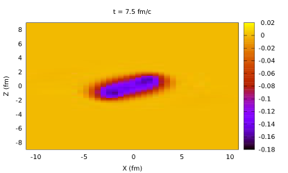
Figure 1: Weighted $\displaystyle y$-component of the vorticity ($\displaystyle c/fm$) averaged over all $\displaystyle x-z$ layers at $\displaystyle 7.5fm/c$, impact parameter $\displaystyle b=8fm$. Average value is $\displaystyle-4.4395\cdot 10^{-2}c/fm$.

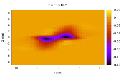
Figure 2: Weighted $\displaystyle y$-component of the vorticity ($\displaystyle c/fm$) averaged over all $\displaystyle x-z$ layers at $\displaystyle 10.5fm/c$, impact parameter $\displaystyle b=8fm$. Average value is $\displaystyle-2.2800\cdot 10^{-2}c/fm$.

Figure 3: Weighted $\displaystyle y$-component of the vorticity ($\displaystyle c/fm$) averaged over all $\displaystyle x-z$ layers at $\displaystyle 14fm/c$, impact parameter $\displaystyle b=8fm$. Average value is $\displaystyle-1.2452\cdot 10^{-2}c/fm$.

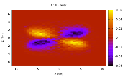
Figure 4: Weighted $\displaystyle y$-component of the vorticity ($\displaystyle c/fm$) averaged over all $\displaystyle x-z$ layers at $\displaystyle 10.5fm/c$, impact parameter $\displaystyle b=0fm$. Average value is $\displaystyle-1.2\cdot 10^{-5}c/fm$.

III.2 Helicity

Figure 5: Helicity: $\displaystyle H_{\uparrow}$ and $\displaystyle H_{\downarrow}$, impact parameter $\displaystyle b=4fm/c$ (a) and $\displaystyle b=8fm/c$ (b).

Main results obtained in HSD model for helicity separation are presented in Figure  5. Simulations in HSD model manifest helicity separation similar to the separation in QGSM model. Along with this there is a notable shift in time (about $\displaystyle 6-7fm/c$). Helicity separation begins later than in helsep0 . This may be explained by the difference in initial state of the nuclei. In the HSD simulation program the nuclei are initial at distance $\displaystyle\leavevmode\nobreak\ 7fm$ apart from each other. Since they start off at a significant distance it takes some time for them to collide .

Magnitudes of $\displaystyle H_{\uparrow}$ and $\displaystyle H_{\downarrow}$ are also different from the same quantities in helsep0 . $\displaystyle H_{\uparrow}$ subdivided by components in scalar product is shown in Figures  5. In both models the $\displaystyle x$ component doesn’t give a significant contribution in $\displaystyle H$. For the QGSM model there is a difference between $\displaystyle y$ and $\displaystyle z$ component contributions. However, there is no such tendency for the HSD model: both components give contribution of similar magnitude.

Figure 6: Results for new derivative formulas parameter $\displaystyle b=4fm/c$.

The same quantity was calculated using another formula for velocity derivatives in helicity for comparison. It can be interesting to see if a more accurate formula can improve the result. Let us calculate derivatives as follows:

$$\partial_{x}v_{\alpha}(m,n,k)=\\ \frac{1}{8h_{x}}\sum_{i=-1,1}\sum_{j=-1,1}\{v_{\alpha}(m+1,n+i,k+j)\\ -v_{\alpha}(m-1,n+i,k+j)\},$$ (1)

$$\partial_{y}v_{\alpha}(m,n,k)=\\ \frac{1}{8h_{y}}\sum_{i=-1,1}\sum_{j=-1,1}\{v_{\alpha}(m+i,n+1,k+j)\\ -v_{\alpha}(m+i,n-1,k+j)\},$$ (2)

$$\partial_{z}v_{\alpha}(m,n,k)=\\ \frac{1}{8h_{z}}\sum_{i=-1,1}\sum_{j=-1,1}\{v_{\alpha}(m+i,n+j,k+1)\\ -v_{\alpha}(m+i,n+j,k-1)\},$$ (3)

where $\displaystyle h_{x},h_{y},h_{z}$ are the cell sizes along $\displaystyle x,y$ and $\displaystyle z$ axis respectively, $\displaystyle m,n,k$ are discrete coordinates on the mesh. This method of calculation uses higher order discrete derivative and averaging over four derivatives calculated at different points. The new formula for derivatives, however, doesn’t give any new or improved results (Figure  6).

Figure 7: Integral values calculated for impact parameter $\displaystyle b=8fm$.

Some integral values have also been computed for additional information and comparison. Plots for these values are presented in Figure 7. Both models give very similar results. However there is a distinct peak on the plot for

$$\frac{(\int(\vec{v},rot\vec{v})dV)^{2}}{\int v^{2}dV\int(rot\vec{v})^{2}dV}$$

in QGSM model, that is missing on the corresponding plot in HSD model. The value eventually decreases but not so rapidly. In both cases this values is very small ( $\displaystyle 10^{-2}-10^{-3}$).

In this section we have studied hydrodynamic vorticity, helicity and some integral values in heavy ion collisions. The results were compared to those that were obtained with the help of QGSM model. They are mostly similar except for an explainable shift in time. Although the integral values are small in magnitude, their time dependence resembles the results obtained in the QGSM model.

The possible observable result of non-zero medium helicity is polarization of $\displaystyle\Lambda$ - hyperons with different signs of $\displaystyle y$ - component of momentum. A quantitive estimate of such polarization is given in helsep0 . At helicity values calculated here and in helsep0 the $\displaystyle\Lambda$ - hyperon polarization is possible to observe. The possibility of $\displaystyle\Lambda$ - hyperon polarization effect is also discussed in Rogachevsky:2010ys . $\displaystyle\Lambda$ - hyperon polarization is considered in hydrodynamic model in lambdapol .

IV Handedness

Since nuclei have non-zero angular momentum in non-central collisions we can expect to find some p-odd effects in the final state. In this part of the article we will try to find relation between properties of particles in the final state with parity in the initial state.

To obtain information about polarization of particles in the initial state based on the properties of particles in the final state several methods were proposed emth nachtm . These methods are based on computation of vector or triple product of 3-momenta of particles in the final state. These methods are suitable for processing experimental data.

In the first article nachtm a pseudoscalar $\displaystyle T$ was introduced:

$$T=\frac{1}{|\vec{p}|}([\vec{p_{1}},\vec{p_{2}}],\vec{p_{3}}),$$

with $\displaystyle|\vec{p_{1}}|>|\vec{p_{2}}|>|\vec{p_{3}}|$, where $\displaystyle\vec{p_{1}}$, $\displaystyle\vec{p_{2}}$ and $\displaystyle\vec{p_{3}}$ - 3-momenta of particles in the final state, $\displaystyle\vec{p}$ - momentum of the particle in the initial state. Using $\displaystyle T$ and quantities derived from it some reactions including electron-positron annihilation to hadrons and nucleon collisions were considered.

Later, in emth a new quantity called handedness was defined. It was proposed to investigate polarization of the initial quark or gluon. Longitudinal handedness is defined as follows:

$$H_{||}=\frac{N_{l}-N_{r}}{N_{l}+N_{r}},$$

where $\displaystyle N_{l}$ and $\displaystyle N_{r}$ - is the number of left- and right-handed combinations $\displaystyle\vec{k}$, $\displaystyle\vec{k_{1}}$, $\displaystyle\vec{k_{2}}$:

$$\begin{cases}e_{ijk}k^{i}k_{1}^{j}k_{2}^{k}>0,&\text{for }N_{l},\\ e_{ijk}k^{i}k_{1}^{j}k_{2}^{k}<0,&\text{for }N_{r}.\end{cases}$$

Here, $\displaystyle\vec{k}$ - momentum of the initial particle, $\displaystyle\vec{k_{1}},\vec{k_{2}}$ - momenta of particles (pions) in the final state. It was proposed to sort particles $\displaystyle\vec{k_{1}}$ and $\displaystyle\vec{k_{2}}$ according to their charge or magnitudes of momenta Two transverse-handedness parameters.

IV.1 Methods and results

Based on these articles we can introduce the following quantity:

$$\eta=\frac{\sum(\vec{p_{3}},\vec{p_{2}},\vec{p_{1}})}{\sum|(\vec{p_{3}},\vec{p_{2}},\vec{p_{1}})|},$$

where $\displaystyle(\vec{p_{3}},\vec{p_{2}},\vec{p_{1}})$ - triple product $\displaystyle(\vec{p_{3}},[\vec{p_{2}},\vec{p_{1}}])$ with all vectors in a triplet in the same octant in the momentum space, $\displaystyle\vec{p_{1}},\vec{p_{2}},\vec{p_{3}}$ - momenta of pions in the final state. Momenta in each triple product were sorted:

$$|p_{3}|^{2}<|p_{2}|^{2}<|p_{1}|^{2}.$$

Hence eight values $\displaystyle\eta_{i},i=0..7$, one for each octant, were calculated. Octants were enumerated the way described in table  1. Au+Au collisions were considered with projectile energy of 5GeV per nucleon in the laboratory frame with impact parameter $\displaystyle b=7fm/c$. Heavy-ion collisions were modelled, as before, in Hadron-String Dynamics model hsdref .

Since collisions are non-central, non-zero values of $\displaystyle\eta$ are expected. To take into account statistical errors, $\displaystyle\eta$ was averaged over a number of events and an estimate of standard deviation for every average value was taken to be the statistical error. Average $\displaystyle\bar{\eta}$ is plotted with the estimate of standard deviation for every octant over $\displaystyle 1/\sqrt{N}$, where $\displaystyle N$ - is the number of events used to calculate the average value (Figures  8 and  9.)

Octant	Momentum
0	$\displaystyle p_{x}>0,p_{y}>0,p_{z}>0$
1	$\displaystyle p_{x}>0,p_{y}>0,p_{z}\leq 0$
2	$\displaystyle p_{x}>0,p_{y}\leq 0,p_{z}>0$
3	$\displaystyle p_{x}>0,p_{y}\leq 0,p_{z}\leq 0$
4	$\displaystyle p_{x}\leq 0,p_{y}>0,p_{z}>0$
5	$\displaystyle p_{x}\leq 0,p_{y}>0,p_{z}\leq 0$
6	$\displaystyle p_{x}\leq 0,p_{y}\leq 0,p_{z}>0$
7	$\displaystyle p_{x}\leq 0,p_{y}\leq 0,p_{z}\leq 0$

Table 1: Octant enumeration.

Figure 8: Dependence of $\displaystyle\bar{\eta}$ on $\displaystyle 1/\sqrt{N}$, for impact parameter $\displaystyle b=7fm$. Octants 1, 3, 4, 6.

Figure 9: Dependence of $\displaystyle\bar{\eta}$ on $\displaystyle 1/\sqrt{N}$, for impact parameter $\displaystyle b=7fm$. Octants 0, 2, 5, 7

Although the statistical error is high at low $\displaystyle N$, we can see that it decreases at higher $\displaystyle N$. As the number of events $\displaystyle N$ increases, $\displaystyle\bar{\eta}$ in octants 1, 3, 4 and 6 does not completely vanish. Moreover $\displaystyle|\bar{\eta}|$ is higher than one standard deviation. This points to the possibility of non-zero values of $\displaystyle\bar{\eta}$ in non-central collisions.

V Conclusion

We have studied vorticity and helicity in heavy-ion collisions in the HSD model for Au+Au reactions at small energy $\displaystyle\sqrt{s}=5GeV$ and for different impact parameters.

Using hydrodynamic approach we calculated the velocity field of the final state particles. Using this velocity field we calculated the averaged weighted voritcity and studied its time evolution. We noticed that the average weighted $\displaystyle y$-component of vorticity decreases over time in non-central heavy-ion collisions and disappears for the central collisions. The spacial distribution averaged over all $\displaystyle x-z$ planes was also considered. The difference of the emerging picture with that in the hydrodynamical approachcshid is due to the viscosity effects.

Helicity separation was observed in the HSD model. The results in this model are similar to those that were obtained in the QGSM model helsep0 , with some differences in time dependence and in magnitude. The most significant discrepancy - in the time dependence can be explained by details of heavy ion collision simulation. At the initial moment of time $\displaystyle t=0$ there is a significant distance between the nuclei, so the reaction happens later. The difference in magnitude isn’t significant. Generally the integral values have similar time dependence, but have smaller magnitude in the HSD model. Non-zero helicity in such reactions can result in $\displaystyle\Lambda$ - hyperon polarization which can be observed.

We have also proposed a pseudoscalar quantity $\displaystyle\eta$ for investigation of parity-odd effects in heavy-ion collisions based on previous suggestions nachtm emth . The advantage of this approach is suitability for experimental observations without additional calculations. Using computer simulations in the HSD model we have obtained preliminary results for $\displaystyle\bar{\eta}(1/\sqrt{N})$ dependence indicating that it could be used to probe for p-odd effects in non-central collisions. Note the ”handedness separation” to the different sides of reaction plane similar to helicity separation discussed above.

Acknowledgements

Authors are grateful to E.L. Bratkovskaya and M. Baznat for help, discussions and comments. O.T. is also thankful to L. P. Csernai, A.V. Efremov, K. Gudima and A.S. Sorin for stimulating discussions and valuable remarks.

References

- (1) D. Kharzeev, K. Landsteiner, A. Schmitt, Ho-Ung Yee, Lect. Notes Phys. 871 (2013)
- (2) O. Rogachevsky, A. Sorin and O. Teryaev, Phys. Rev. C 82, (2010) 054910 [arXiv:1006.1331 [hep-ph]].
- (3) M. Baznat, K. Gudima, A. Sorin and O. Teryaev, Phys. Rev. C 88, (2013) 061901 [arXiv:1301.7003 [nucl-th]].
- (4) L. P. Csernai, V. K. Magas and D. J. Wang, Phys. Rev. C 87 (2013) 3, 034906 [arXiv:1302.5310 [nucl-th]].
- (5) W. Cassing and E.L. Bratkovskaya, Phys. Reports 308 (1999) 65.
- (6) F. Becattini, L. Csernai, D. J. Wang Phys.Rev. C88 (2013) 034905
- (7) A.V. Efremov, L. Mankiewicz, N.A. Trnqvist, Physics Letters B 284 (1992) 394-400
- (8) Otto Nachtmann, Nuclear Physics B127 (1977) 314-330