Entrainment by spatiotemporal chaos in glow discharge-semiconductor systems

Abstract

Entrainment of limit cycles by chaos [1] is discovered numerically through specially designed unidirectional coupling of two glow discharge-semiconductor systems. By utilizing the auxiliary system approach [2], it is verified that the phenomenon is not a chaos synchronization. Simulations demonstrate various aspects of the chaos appearance in both drive and response systems. Chaotic control is through the external circuit equation and governs the electrical potential on the boundary. The expandability of the theory to collectives of glow discharge systems is discussed, and this increases the potential of applications of the results. Moreover, the research completes the previous discussion of the chaos appearance in a glow discharge-semiconductor system [3].

Keywords: Glow discharge; Plasma; Spatiotemporal chaos; Entrainment by chaos; Period-doubling cascade; Cyclic chaos; Unidirectional coupling; Generalized synchronization.

Spatiotemporal chaos is one of the complicated structures observed in spatially extended dynamical systems and it is characterized by chaotic properties both in time and space coordinates. The existence of a positive Lyapunov exponent can be used to detect spatiotemporal complexity, which can be observed, for example, in liquid crystal light valves, electroconvection, cardiac fibrillation, chemical reaction-diffusion systems and fluidized granular matter. Spatially extended dynamical systems often serve as standard models for the investigation of complex phenomena in electronics. A special interest is directed towards pattern-formation phenomena in electronic media, mainly the nonlinear gas discharge systems. It is clear that chaos can appear as an intrinsic property of systems as well as through couplings. The interaction of spatially extended systems is important for neural networks, reentry initiation in coupled parallel fibers, thermal convection in multilayered media and for systems consisting of several weakly coupled spatially extended systems such as the electrohydrodynamical convection in liquid crystals. In the present study, we numerically verify the appearance of cyclic irregular behavior (entrainment by chaos) in unidirectionally coupled glow discharge-semiconductor systems. The chaos in the response system is obtained through period-doubling cascade of the drive system such that it admits infinitely many unstable periodic solutions and sensitivity is present. Previously, the extension of chaos through couplings has been considered by synchronization [2], [4]-[9]. The task is difficult for partial differential equations because of the choice of connecting parameters [10]-[12]. Kocarev et al. [10] suggested a useful time-discontinuous monitoring for synchronization, but our choice is based on a finite dimensional connection. It is demonstrated that the present results cannot be reduced to any one in the theory of synchronization of chaos. The technique of chaos extension suggested in the present research can be related to technical problems [13, 14], where collectives of microdischarge systems are considered and in models which appear in neural networks, hydrodynamics, optics, chemical reactions and electrical oscillators. Stabilization of multidimensional periodical regimes can be useful in applications of the glow discharge systems in conventional and energy saving lamps, beamers, flat TV screens, etc.

1 Introduction

The investigations of chaos theory for continuous-time dynamics started due to the needs of real world applications, especially with the studies of Poincaré [15], Cartwright and Littlewood [16], Levinson [17], Lorenz [18] and Ueda [19]. Chaotic dynamics has high effectiveness in the analysis of electrical processes of neural networks [20, 21] and can be used for optimization and self-organization problems in robotics [22]. The reason for that is the opportunities provided by the dynamical structure of chaos.

Starting from the primary investigations [16]-[19], chaos has been found as an internal property of systems, and studies in this sense have prolonged until today, for example, by the construction of discrete maps [23]-[26]. At the very beginning of the chaos analysis one has to mention the Smale Horseshoes technique [27] and symbolic dynamics [28]. Another opportunity to reveal chaotic dynamics is the usage of bifurcation diagrams [29, 30].

If one considers a mechanical or electrical system and perturb it by an external force which is bounded, periodic or almost periodic, then the forced system can produce a behavior with a similar property, boundedness/periodicity/almost periodicity [31]-[35]. A reasonable question appears whether it is possible to use a chaotic force to obtain the same type of irregularity in physical systems.

To meet the challenge, we introduced rigorous description of chaotic force as a function or a set of functions and described the input-output mechanism for ordinary differential equations in the studies [1], [36]-[47]. It was rigorously proved that an irregular behavior can follow the chaotic force very likely as regular motions do. We have applied the machinery to mechanical and electrical systems with a finite number of freedom [1], [42]-[45] as well as to neural networks [46, 47]. In the present study, we apply the theory to unidirectionally coupled glow discharge-semiconductor (GDS) systems.

1.1 Preliminaries of the chaos extension

Chaotic dynamics can appear in systems as an intrinsic property and it can be extended through interactions. In the literature, an effective and unique way of the chaos extension from one system to another has been suggested within the scope of generalized synchronization [2], [4]-[8], which characterizes the dynamics of a response system that is driven by the output of a chaotic driving system. Suppose that the dynamics of the drive and response systems are governed by the following systems with a skew product structure

$$x^{\prime}=F(x)$$ (1.1)

and

$$y^{\prime}=G(y,H(x)),$$ (1.2)

respectively, where $x\in\mathbb{R}^{m},y\in\mathbb{R}^{n}.$ Generalized synchronization is said to occur if there exist sets $I_{x},I_{y}$ of initial conditions and a transformation $\phi,$ defined on the chaotic attractor of (1.1), such that for all $x(0)\in I_{x}$ and $y(0)\in I_{y}$ the relation $\displaystyle\lim_{t\to\infty}\left\|y(t)-\phi(x(t))\right\|=0$ holds. In that case, a motion which starts on $I_{x}\times I_{y}$ collapses onto a manifold $M\subset I_{x}\times I_{y}$ of synchronized motions. The transformation $\phi$ is not required to exist for the transient trajectories. When $\phi$ is the identity, the identical synchronization takes place [8, 9].

The synchronization of a large class of unidirectionally coupled chaotic partial differential equations was deeply investigated in [10, 11], where the synchronization was achieved by applying the driving signals only at a finite number of space points. The synchronization of spatiotemporal chaos in a pair of complex Ginzburg-Landau equations was performed in [12] for the case when all space points are continuously driven. In the present study, we use perturbations to a single coordinate of an infinite dimensional response system, which is non-chaotic in the absence of driving, to obtain chaotic motions in the system.

It has not been investigated whether the response system admits the same type of chaos with the drive system in the theory of chaos synchronization yet. The replication of chaos with specific types such as Devaney [48], Li-Yorke [23] and period-doubling cascade [49]-[51] was investigated for drive-response couples for the first time in our papers [1], [36]-[47].

In the study [1], we considered a system of the form

$$u^{\prime}=K(u),$$ (1.3)

where $K:\mathbb{R}^{n}\to\mathbb{R}^{n}$ is a continuously differentiable function. We supposed that system (1.3) possesses an orbitally stable limit cycle and perturbed it with solutions of a chaos generating system, in the form of (1.1), and set up the system

$$y^{\prime}=K(y)+\mu M(x),$$ (1.4)

where $\mu$ is a nonzero number and $M:\mathbb{R}^{m}\to\mathbb{R}^{n}$ is a continuous function. The extension of sensitivity and chaos through period-doubling cascade for the coupled system (1.1)-(1.4) were rigorously proved in the paper [1]. As a result, we achieved chaotic cycles, that is, motions which behave cyclically and chaotically, simultaneously.

The rich experience of chaos expansion in finite dimensional spaces provides a confidence that our approach mentioned in [1] has to work also in infinite dimensional spaces. In this paper, we numerically observe the presence of orbitally stable limit cycles in the $2-$dimensional projections of the infinite dimensional space as well as their deformation to chaotic cycles under chaotic perturbations. By using the technique presented in [1], one can elaborate the results of the present study from the theoretical point of view. Although couplings of GDS systems have not been performed in the literature yet, our results reveal the opportunity of chaos extension in such systems.

Summarizing, electronic systems are important tools for synchronization and chaos extension. In this paper, we make use of our previous approach [1] to extend chaos in unidirectionally coupled GDS systems.

1.2 Description of the GDS system model

Our GDS was previously studied both theoretically and experimentally in [3], [52]-[66]. It represents a planar plasma layer coupled to a planar semiconductor layer, which are sandwiched between two planar electrodes to which a DC voltage is applied (see Fig. 1). We used one-dimensional fluid model for this system, where any pattern formation in the transversal direction is excluded and only the single dimension normal to the layers is resolved. For the gas discharge, the model takes into account electron and ion drift in the electric field, bulk impact ionization and secondary emission from the cathode as well as space charge effects. The semiconductor is approximated with a constant conductivity.

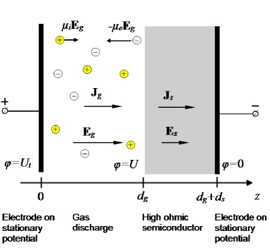
Figure 1: A cross section of a planar discharge cell: it consist of a metal anode, a gas layer, a high-ohmic cathode, and another metal contact. The subscripts $g$ and $s$ refer to the gas and semiconductor regions.

The gas-discharge part of the model consists of continuity equations for two charged species, namely, electrons and positive ions with particle densities $n_{\rm e}$ and $n_{i}$:

$$\partial{{}_{t}}n_{\rm e}+\nabla\cdot{\bf\Gamma}_{\rm e} = {\it S_{e}},$$ (1.5)

$$\partial{{}_{t}}n_{i}+\nabla\cdot{\bf\Gamma}_{i} = {\it S_{i}},$$ (1.6)

which are coupled to Poisson’s equation for the electric field in electrostatic approximation:

$$\nabla\cdot{\bf E}=\frac{e}{\varepsilon_{0}}\left(n_{i}-n_{\rm e}\right),~{}~{}{\bf E}=-\nabla{\Phi}.$$ (1.7)

Here, $\Phi$ is the electric potential, ${\bf E}$ is the electric field in the gas discharge, $e$ is the elementary charge, and $\varepsilon_{0}$ is the dielectric constant. The vector fields ${\bf\Gamma}_{\rm e}$ and ${\bf\Gamma}_{i}$ are the particle flux densities, that in simplest approximation are described by drift only. (In general, particle diffusion $D_{e,i}\nabla n_{e,i}$ could be included.) The drift velocities are assumed to depend linearly on the local electric field with mobilities $\mu_{e}\gg\mu_{i}$:

$${\bf\Gamma}_{\rm e}=-\mu_{\rm e}n_{\rm e}\,{\bf E},~{}~{}~{}{\bf\Gamma}_{i}=\mu_{i}n_{i}\,{\bf E},$$ (1.8)

hence the total electric current in the discharge is

$${\bf J}=\epsilon_{0}\partial_{t}{\bf E}+e\,\big{(}{\bf\Gamma}_{i}-{\bf\Gamma}_{\rm e}\big{)}=\epsilon_{0}\partial_{t}{\bf E}+e\,\Big{(}\mu_{i}n_{i}+\mu_{\rm e}n_{\rm e}\Big{)}\,{\bf E}.$$ (1.9)

Two types of ionization processes are taken into account: the $\alpha$ process of electron impact ionization in the bulk of the gas, and the $\gamma$ process of electron emission by ion impact onto the cathode. In a local field approximation, the $\alpha$ process determines the source terms in the continuity equations (1.5) and (1.6):

$${\it S_{e}}={\it S_{i}}=|{\bf\Gamma}_{\rm e}|\,\alpha_{0}\,\alpha\left({|{\bf E}|}/{E_{0}}\right),$$ (1.10)

where we use the classical Townsend approximation

$$\alpha\left(|{\bf E}|/E_{0}\right)=\exp\left(-E{{}_{0}}/|{\bf E}|\right).$$ (1.11)

The effect of the semiconductor layer with thickness $d_{s}$, conductivity $\sigma_{s}$, dielectric constant $\varepsilon_{s}$ is described by the external circuit equation

$$\partial_{t}U=\frac{U_{t}-U-R_{s}J}{T_{s}},$$ (1.12)

where $U_{t}$ is the applied voltage, $U=\int_{0}^{d_{g}}E\,dZ$ is the voltage over the gas discharge which is the electric field $E$ integrated over the height $d_{g}$ of the discharge, $R_{s}=d_{s}/\sigma_{s}$ is the resistance of the semiconductor layer, where $\sigma_{s}$ is its conductivity, and $T_{s}=\epsilon_{s}\epsilon_{0}/\sigma_{s}$ is the Maxwell relaxation time of the semiconductor with dielectric constant $\varepsilon_{s}$.

Following the traditions of the synchronization of chaotic systems, we will call the coupled GDS systems as the drive and response systems.

The goal of our investigation is to extend the spatiotemporal chaos of a drive GDS system to a response GDS system by means of a special connection mechanism between the systems. In order to make our present study self-sufficient, we complete the chaos analysis of the GDS system, which was initiated in the papers [3, 52]. The method of the analysis, as well as the connection mechanism are our theoretical suggestions [1], [36]-[47] and in the present circumstances one can say that we consider entrainment by chaos [1] for GDS systems. Entrainment by chaos, which is the deformation of limit cycles to chaotic cycles, is verified by simulations.

The chaos obtained through period-doubling cascade [49]-[51] is under investigation in the present study. In other words, the existence of infinitely many unstable periodic solutions and the presence of sensitivity [48] are considered. One of the advantages of our approach is the controllability of the extended chaos [1, 8, 42, 43, 67]. It is possible to stabilize an unstable periodic solution of the response GDS system by controlling the chaos of the drive system. The presented technique is applicable to large number interconnected GDS systems and the control of the global chaos can also be achieved. This approach can be useful for applications of the gas discharge systems in conventional and energy saving lamps, beamers, flat TV screens, etc. [13, 14].

1.3 Formulation of the model in dimensionless form

The dimensional analysis is performed essentially as in [3, 52]. In dimensional units, $Z$ parametrizes the direction normal to the layers. The anode of the gas discharge is at $Z=0$, the cathode end of the discharge is at $Z=d_{g}$, and the semiconductor extends up to $Z=d_{g}+d_{s}$.

When diffusion is neglected, the ion current and the ion density at the anode vanish. This is described by the boundary condition on the anode $Z=0$:

$${\bf\Gamma}_{i}\left(0,t\right)=0~{}~{}~{}\Rightarrow~{}~{}~{}n_{i}\left(0,t\right)=0.$$ (1.13)

The boundary condition at the cathode, $Z=d_{g}$, describes the $\gamma$-process of secondary electron emission:

$$\left|{\bf\Gamma}_{\rm e}\left(d_{g},t\right)\right|=\gamma\left|{\bf\Gamma}_{i}\left(d_{g},t\right)\right|~{}~{}~{}\Rightarrow~{}~{}~{}\mu_{\rm e}n_{\rm e}\left(d_{g},t\right)=\gamma\mu_{i}n_{i}\left(d_{g},t\right).$$ (1.14)

Finally, a DC voltage $U_{t}$ is applied to the system determining the electric potential on the boundaries

$$\Phi\left(0,t\right)=0,~{}~{}~{}\Phi\left(d_{g},t\right)=-U.$$ (1.15)

Here, the first potential vanishes due to gauge freedom.

Let us introduce the intrinsic parameters of the system as $\displaystyle t_{0}=\frac{1}{\alpha_{0}\mu_{e}E_{0}},$ $\displaystyle Z_{0}=\frac{1}{\alpha_{0}},$ $\displaystyle n_{0}=\frac{\varepsilon_{0}\alpha_{0}E_{0}}{e}.$ In the studies [3, 52], the problem was reduced to one spatial dimension $z$ such that the GDS system takes the following dimensionless form,

$$\begin{array}[]{l}\partial_{\tau}\sigma-\partial_{z}\left(\cal{E}\sigma\right)=\sigma\cal{E}\alpha\left(\cal{E}\right),\\ \partial_{\tau}\rho+\mu\partial_{z}\left(\cal{E}\rho\right)=\sigma\cal{E}\alpha\left(\cal{E}\right),\\ \partial_{z}{\cal{E}}=\rho-\sigma,~{}~{}{\cal{E}}=-\partial_{z}\phi,\end{array}$$ (1.19)

where the dimensionless time, coordinates and fields are $\displaystyle{z}=\frac{{Z}}{Z_{0}},$ $\displaystyle\tau=\frac{t}{t_{0}},$ $\displaystyle\sigma({z},\tau)=\frac{n_{\rm e}\left({Z},t\right)}{n_{0}},$ $\displaystyle\rho({z},\tau)=\frac{n_{i}\left({Z},t\right)}{n_{0}},$ $\displaystyle{\cal{E}}({z},\tau)=\frac{{E}\left({Z},t\right)}{E_{0}},$ $\displaystyle\phi({z},\tau)=\frac{\Phi\left({Z},t\right)}{E_{0}Z_{0}}$ and $\displaystyle\alpha\left(\cal{E}\right)=e^{-1/|{\cal{E}}|}.$

The intrinsic dimensionless parameters of the gas discharge are the mobility ratio $\mu$ of electrons and ions and the length ratio $L$ of discharge gap width and impact ionization length. That is, $\displaystyle\mu=\frac{\mu_{i}}{\mu_{e}}$ and $L=\displaystyle\frac{d_{g}}{Z_{0}}.$ The boundary conditions become

$$\begin{array}[]{l}\rho(0,\tau)=0,\\ \sigma(L,\tau)=\gamma\mu\rho(L,\tau),\\ \phi(0,\tau)=0,~{}~{}\phi(L,\tau)=-{\cal{U}},\end{array}$$ (1.23)

and the external circuit is described by

$$\partial_{\tau}{\cal{U}}=\frac{{\cal{U}}_{t}-{\cal{U}}-{\cal{R}}_{s}j}{\tau_{s}},$$ (1.24)

where the total applied voltage is rescaled as ${\cal U}_{t}={U_{t}}/({E_{0}Z_{0}})$, dimensionless voltage ${\cal{U}}(\tau)=\int_{0}^{L}{\cal{E}}\,dz$, time scale $\tau_{s}=T_{s}/t_{0}$, resistance ${\cal{R}}_{s}=R_{s}\,e\mu_{e}n_{0}/Z_{0}$, and spatially conserved total current $j(\tau)=\partial_{\tau}{\cal{E}}+\mu\rho{\cal{E}}+\sigma{\cal{E}}$.

We consider a regime corresponding to a transition between Townsend and glow discharge. The parameters are taken as in the experiments [62] and in our previous work [3]. The discharge is in nitrogen at 40 mbar, in a gap of 1.4 mm. We used the ion mobility $\mu_{i}=23.33~{}{\rm cm^{2}/(V\,s)}$ and electron mobility $\mu_{e}=6666.6~{}{\rm cm^{2}/(V\,s)}$, therefore the mobility ratio is $\mu=\mu_{i}/\mu_{e}=0.0035$. The secondary emission coefficient was taken as $\gamma=0.08$. The applied voltages $U_{t}$ are in the range of 513–570 V. For $\alpha_{0}=Ap=[27.8\;\mu{\rm m}]^{-1}$ and for $E_{0}=Bp=10.3\;{\rm kV/cm}$, we used values from [57]. The semiconductor layer consists of 1.5 mm of GaAs with dielectric constant $\varepsilon_{s}=13.1$ and conductivity $\sigma_{s}=(2.6\times 10^{5}~{}\Omega\,{\rm cm})^{-1}$. Corresponding dimensionless parameters are $L=50$, ${\cal{R}}_{s}=30597$, $\tau_{s}=7435$, and a total voltage range ${\cal{U}}_{t}$ between $17.67$ and $20.03.$

2 Chaotically coupled GDS systems

In the present section, we will extend the spatiotemporal chaos of a drive GDS system through utilizing its voltage over the gas discharge as a chaotic control applied to the electric circuit of a response GDS system. In the coupling, the voltage over the discharge of the drive system is applied as a perturbation to the circuit equation of the response system. The presence of entrainment by chaos in the response system will be shown numerically. Moreover, we will compare our results with generalized synchronization.

The full analysis of the spatiotemporal chaos in the GDS system (1.19-1.24) is provided in the Appendix, where the bifurcation diagram as well as the chaotic behaviors in the voltage, electric field, electron density and ion density of the system are represented. According to these results, the GDS system

$$\begin{array}[]{l}\partial_{\tau}\sigma-\partial_{z}\left(\cal{E}\sigma\right)=\sigma\cal{E}\alpha\left(\cal{E}\right),\\ \partial_{\tau}\rho+\mu\partial_{z}\left(\cal{E}\rho\right)=\sigma\cal{E}\alpha\left(\cal{E}\right),\\ \partial_{z}{\cal{E}}=\rho-\sigma,~{}~{}{\cal{E}}=-\partial_{z}\phi,\\ \displaystyle\partial_{\tau}{\cal{U}}=\frac{20-{\cal{U}}-{\cal{R}}_{s}j}{\tau_{s}},\end{array}$$ (2.29)

is chaotic, and it will be accompanied by the boundary conditions

$$\rho(0,\tau)=0,$$

$$\sigma(L,\tau)=\gamma\mu\rho(L,\tau),$$

$$\phi(0,\tau)=0,~{}~{}\phi(L,\tau)=-{\cal{U}}.$$

We will take into account (2.29) as the drive system.

The solutions of (2.29) will be used as a perturbation for the response GDS system in the form,

$$\begin{array}[]{l}\partial_{\tau}\widetilde{\sigma}-\partial_{z}\left(\widetilde{\cal{E}}\widetilde{\sigma}\right)=\widetilde{\sigma}\widetilde{\cal{E}}\alpha\left(\widetilde{\cal{E}}\right),\\ \partial_{\tau}\widetilde{\rho}+\mu\partial_{z}\left(\widetilde{\cal{E}}\widetilde{\rho}\right)=\widetilde{\sigma}\widetilde{\cal{E}}\alpha\left(\widetilde{\cal{E}}\right),\\ \partial_{z}{\widetilde{\cal{E}}}=\widetilde{\rho}-\widetilde{\sigma},~{}~{}{\widetilde{\cal{E}}}=-\partial_{z}\widetilde{\phi},\\ \displaystyle\partial_{\tau}{\cal{V}}=\frac{{\cal V}_{t}-{\cal V}-{\cal{R}}_{s}\widetilde{j}+\delta{\cal{U}}(\tau)}{\tau_{s}},\end{array}$$ (2.34)

with the boundary conditions

$$\widetilde{\rho}(0,\tau)=0,$$

$$\widetilde{\sigma}(L,\tau)=\gamma\mu\widetilde{\rho}(L,\tau),$$

$$\widetilde{\phi}(0,\tau)=0,~{}~{}\widetilde{\phi}(L,\tau)=-{\cal{V}}.$$

In system (2.34), $\delta$ is a nonzero number and the term $\delta{\cal U}(\tau)/\tau_{s}$ is the perturbation from the drive system (2.29).

It is shown in the Appendix for the parameter value ${\cal U}_{t}=17.7$ that the projection of the attractor of system (1.19)-(1.24) on the domain of equation (1.24) is a stable limit cycle (see Fig. 8). That is, in the absence of driving, the response system (2.34) with ${\cal V}_{t}=17.7$ does not possess chaos. We will numerically show that the response GDS system possesses chaotic motions near the limit cycle, provided that the driving effect is included. Our results are theoretically based on the study [1], where we have proved that if the drive system admits infinitely many unstable periodic solutions and sensitivity, then the response system does the same. Since the attractor exists in system (1.19)-(1.24) with ${\cal U}_{t}=17.7$, one can conclude by the extension of our results presented in [1] that if the number $|\delta|$ in equation (2.34) is sufficiently small, then system (2.34) possesses cyclic chaos. That is, entrainment by chaos takes place in the system.

Let us take ${\cal V}_{t}=17.7$ and $\delta=0.047$ in the response GDS system (2.34). Using the solution of the drive system shown in Figures 9, 10 and 11, we depict in Figure 2 the projection of a chaotic solution of (2.34) on the ${\cal V}-\widetilde{j}$ plane. On the other hand, the projection of the stroboscopic plot of the response system on the same plane is shown in Figure 3. Both of the figures reveal that the response GDS system possesses motions that behave chaotically around the limit cycle of system (1.19)-(1.24) with ${\cal U}_{t}=17.7.$ Moreover, to support the presence of chaos in the response system, we depict in Figure 4 the time series of the $\cal V$ coordinate. The amplitude ranges $15-16.6$ and $7.4-8.6$ are used in Figure 4, (b) and (c), respectively, to increase the visibility of chaotic behavior.

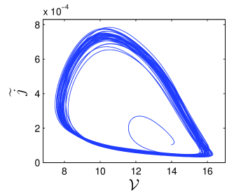
Figure 2: The trajectory of the response system (2.34) in the ${\cal V}-\widetilde{j}$ plane manifests the chaotic cycle.

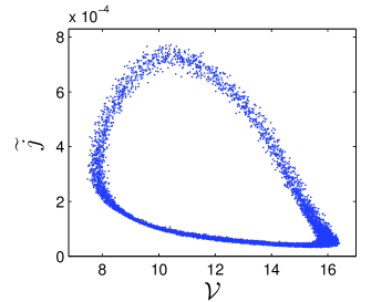
Figure 3: The projection of the stroboscopic plot of system (2.29)-(2.34) on the ${\cal V}-\widetilde{j}$ plane reveals the presence of chaotic behavior in the response system.

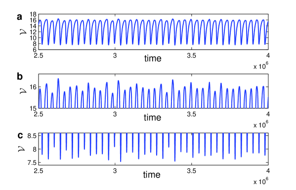
Figure 4: The behavior of the $\cal V$ coordinate of system (2.34) is shown in (a). In (b) and (c), where the chaotic behavior is observable, the amplitudes are restricted to the ranges $15-16.6$ and $7.4-8.6,$ respectively.

Figure 5, (a), (b) and (c) depict, respectively, the chaotic behavior in the electric field, electron density and ion density of system (2.34). These figures also support the presence of motions that behave chaotically around the limit cycle.

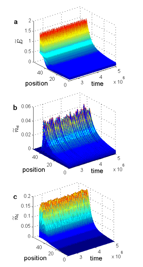
Figure 5: Time evolution of profiles of the (a) electric field $\widetilde{E},$ (b) electron density $\widetilde{n}_{e},$ and (c) ion density $\widetilde{n}_{i}$ support the existence of chaotic motions around the periodic solution.

Now, let us compare our results with generalized synchronization (GS) [4]-[8]. According to Kocarev and Parlitz (1996), GS occurs for the coupled systems (1.1) and (1.2) if and only if for all $x_{0}\in I_{x},$ $y_{10},$ $y_{20}\in I_{y},$ the asymptotic stability criterion $\displaystyle\lim_{t\to\infty}\left\|y(t,x_{0},y_{10})-y(t,x_{0},y_{20})\right\|=0$ holds, where $y(t,x_{0},y_{10})$ and $y(t,x_{0},y_{20})$ denote the solutions of (1.2) with the initial data $y(0,x_{0},y_{10})=y_{10},$ $y(0,x_{0},y_{20})=y_{20}$ and the same $x(t),$ $x(0)=x_{0}.$ This criterion is a mathematical formulation of the auxiliary system approach [2, 8]. We shall make use of the auxiliary system approach to demonstrate the absence of generalized synchronization in the coupled system (2.29)-(2.34).

We introduce the auxiliary system

$$\begin{array}[]{l}\partial_{\tau}\overline{\sigma}-\partial_{z}\left(\overline{\cal{E}}\overline{\sigma}\right)=\overline{\sigma}\overline{\cal{E}}\alpha\left(\overline{\cal{E}}\right),\\ \partial_{\tau}\overline{\rho}+\mu\partial_{z}\left(\overline{\cal{E}}\overline{\rho}\right)=\overline{\sigma}\overline{\cal{E}}\alpha\left(\overline{\cal{E}}\right),\\ \partial_{z}{\overline{\cal{E}}}=\widetilde{\rho}-\overline{\sigma},~{}~{}{\overline{\cal{E}}}=-\partial_{z}\overline{\phi},\\ \displaystyle\partial_{\tau}{\cal{W}}=\frac{17.7-{\cal{W}}-{\cal{R}}_{s}\overline{j}+0.047\cal{U}(\tau)}{\tau_{s}}\end{array}$$ (2.39)

with the boundary conditions

$$\overline{\rho}(0,\tau)=0,$$

$$\overline{\sigma}(L,\tau)=\gamma\mu\overline{\rho}(L,\tau),$$

$$\overline{\phi}(0,\tau)=0,~{}~{}\overline{\phi}(L,\tau)=-{\cal{W}}.$$

Making use of the solution ${\cal U(\tau)}$ whose graph is represented in Figure 10 in both of the systems (2.34) and (2.39), we depict in Figure 6 the projection of the stroboscopic plot of system (2.34)-(2.39) on the ${\cal V}-{\cal W}$ plane. The first $500$ iterations are omitted in the simulation. The time interval $[0,80\times 10^{6}]$ is used and the time step is taken as $\Delta\tau=5000.$ Since the plot does not take place on the line ${\cal W}={\cal V},$ we conclude that generalized synchronization is not achieved in the dynamics of the coupled system (2.29)-(2.34).

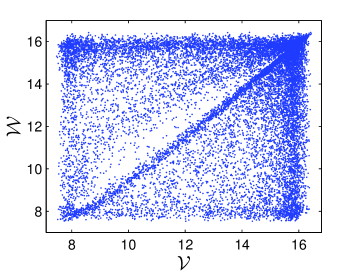
Figure 6: Application of the auxiliary system approach reveals that the coupled systems (2.29) and (2.34) are not synchronized.

3 Conclusions

In the studies [1], [36]-[47], we applied the input-output mechanism to systems that admit stable equilibrium points as well as limit cycles. It is theoretically proved in [1] that weak forcing of systems with stable limit cycles leads to the deformation of limit cycles to chaotic cycles, that is motions that behave chaotically around the limit cycle. This phenomenon, which is called entrainment by chaos, cannot be explained by the theory of generalized synchronization [4]-[8], and it is also used in the present study. In the electrical sense, the chaotification of limit cycles is much more preferable than that procedure for asymptotic equilibria, because of the role of oscillations for electronics. Accordingly, in this paper, we demonstrate the entrainment by chaos in coupled glow discharge systems.

In this paper, we utilize GDS systems as drive and response electrical models. GDS systems were analyzed for a chaos presence in [3]. We complete the analysis by constructing the full period-doubling bifurcation diagram to demonstrate that the drive system admits infinitely many unstable periodic solutions as well as sensitivity. However, this is only an auxiliary result. The main novelty of the present article with respect to the previous studies [3, 52, 53] is that we consider these systems which are coupled in a unidirectional way and prove that the chaos can be extended through couplings of GDS systems as well as in their arbitrary large collectives. This type of chaos extension may give benefits in further applications, for example, in economic lamps and flat TV screens [13, 14]. We suggest that our way of numerical analysis and special design of complexity can be further verified experimentally. It is worth noting that our approach is not generalized synchronization of chaos at all. This is demonstrated through the special method of auxiliary system approach [2, 8].

Appendix: The chaos in the drive GDS system

In this part, we will extend the results of [3] about the presence of chaos in GDS systems. In the article [3], only a finite number of period-doubling bifurcations were indicated. However, in the present study, we represent the occurrence of infinitely many period-doubling bifurcations by means of a bifurcation diagram and we definitely reveal the regions of regularity and chaoticity.

The bifurcation diagram corresponding to the ${\cal U}$ coordinate of system (1.19)-(1.24) with the boundary conditions (1.23) is pictured in Figure 7. Here, ${\cal U}_{t}$ is the bifurcation parameter. Supporting the results of [3], it is observable in the figure that the system displays period-doubling bifurcations and leads to chaos. The period-doubling bifurcations occur approximately at the ${\cal U}_{t}$ values $18.315,$ $18.782,$ $18.902,$ $18.939,$ etc., and a period-six window appears near ${\cal U}_{t}=19.073$ in the bifurcation diagram.

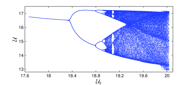
Figure 7: The bifurcation diagram of system (1.19)-(1.24) for the values of the parameter ${\cal U}_{t}$ between $17.67$ and $20.03$.

One can conclude from the bifurcation diagram that the system (1.19)-(1.24) possesses a stable periodic solution for ${\cal U}_{t}=17.7.$ The projection of a solution that approaches to the stable limit cycle, which is the projection of the attractor of the global system (1.19)-(1.24) on the domain of (1.24) with ${\cal U}_{t}=17.7,$ is depicted in Figure 8. This result confirms the existence of an attractor as a periodic solution in the spatiotemporal equation.

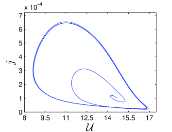
Figure 8: The figure reveals a limit cycle, the projection of the attractor of the global system on the domain of equation (1.24) with ${\cal U}_{t}=17.7.$

The bifurcation diagram shown in Figure 7 confirms that the drive GDS system (2.29) is chaotic. The projection of a chaotic solution of (2.29) on the ${\cal U}-j$ plane is represented in Figure 9. Moreover, the time series of the ${\cal U}$ coordinate of the same solution is shown Figure 10, where one can see the chaotic behavior.

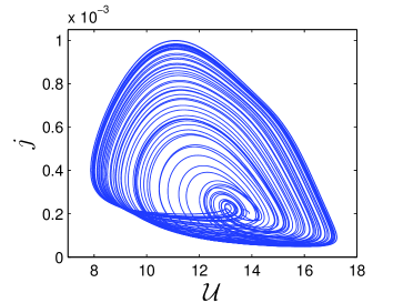
Figure 9: The projection of the chaotic solution of the drive GDS system (2.29) on the ${\cal U}-j$ plane.

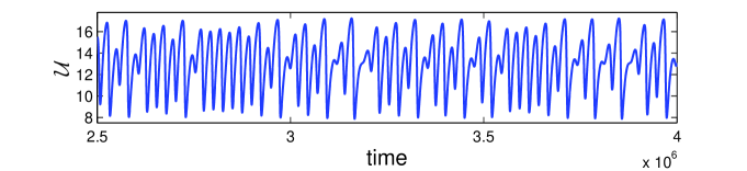
Figure 10: The chaotic behavior of the $\cal U$ coordinate of system (2.29).

The profiles of the electric field $E$, electron density $n_{\rm e}$ and ion density $n_{i}$ of (2.29) are pictured in Figure 11, (a), (b) and (c), respectively. Figure 11 also confirms the presence of chaos in the drive system.

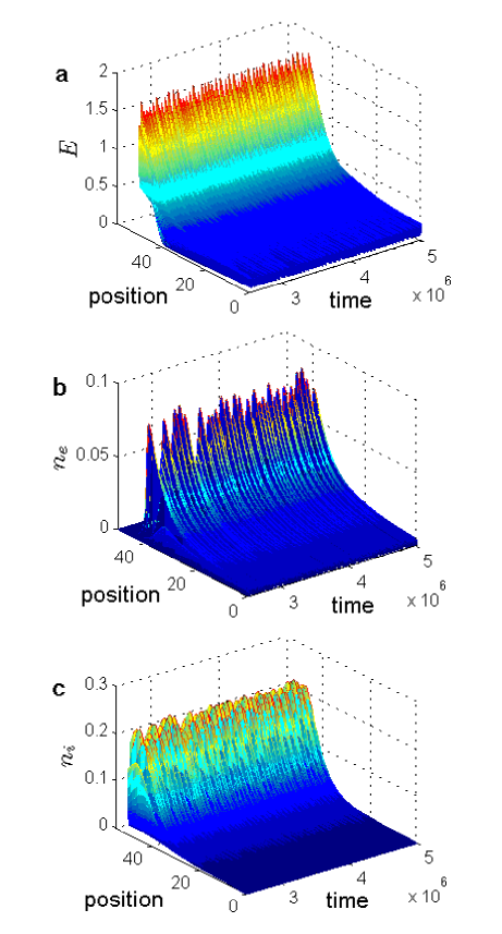
Figure 11: Profiles of the (a) electric field $E,$ (b) electron density $n_{e},$ and (c) ion density $n_{i}$ as functions of time support the existence of spatiotemporal chaos.

References

- [1] M. U. Akhmet and M. O. Fen, “Entrainment by chaos,” Journal of Nonlinear Science 24, 411-439 (2014).
- [2] H. D. I. Abarbanel, N. F. Rulkov, and M. M. Sushchik, “Generalized synchronization of chaos: The auxiliary system approach,” Phys. Rev. E 53, 4528-4535 (1996).
- [3] D. D. Šijačić, U. Ebert, and I. Rafatov, “Period doubling cascade in glow discharges: Local versus global differential conductivity,” Phys. Rev. E 70, 056220 (2004).
- [4] N. F. Rulkov, M. M. Sushchik, L. S. Tsimring, and H. D. I. Abarbanel, “Generalized synchronization of chaos in directionally coupled chaotic systems,” Phys. Rev. E 51, 980-994 (1995).
- [5] L. Kocarev and U. Parlitz, “Generalized synchronization, predictability, and equivalence of unidirectionally coupled dynamical systems,” Phys. Rev. Lett. 76, 1816-1819 (1996).
- [6] B. R. Hunt, E. Ott, and J. A. Yorke, “Differentiable generalized synchronization of chaos,” Phys. Rev. E 55, 4029-4034 (1997).
- [7] U. S. Freitas, E. E. N. Macau, and C. Grebogi, “Using geometric control and chaotic synchronization to estimate an unknown model parameter,” Phys. Rev. E 71, 047203 (2005).
- [8] J. M. Gonzáles-Miranda, Synchronization and Control of Chaos, Imperial College Press, London, 2004.
- [9] L. M. Pecora and T. L. Carroll, “Synchronization in chaotic systems,” Phys. Rev. Lett. 64, 821-825 (1990).
- [10] L. Kocarev, Z. Tasev, and U. Parlitz, “Synchronizing spatiotemporal chaos of partial differential equations,” Phys. Rev. Lett. 79, 51-54 (1997).
- [11] L. Kocarev, Z. Tasev, T. Stojanovski, and U. Parlitz, “Synchronizing spatiotemporal chaos,” Chaos 7, 635-643 (1997).
- [12] M.M. Sushchik, Ph.D. dissertation, University of California, San Diego, 1996.
- [13] U. Kogelschatz, “Filamentary, patterned, and diffuse barrier discharges,” IEEE Trans. Plasma Science 30, 1400-1408 (2002).
- [14] U. Kogelschatz, “Dielectric-barrier discharges: Their history, discharge physics, and industrial applications,” Plasma Chemistry and Plasma Processing 23, 1-46 (2003).
- [15] K. G. Andersson, “Poincaré’s discovery of homoclinic points,” Archive for History of Exact Sciences 48, 133-147 (1994).
- [16] M. Cartwright and J. Littlewood, “On nonlinear differential equations of the second order I: The equation large,” J. London Math. Soc. 20, 180-189 (1945).
- [17] N. Levinson, “A second order differential equation with singular solutions,” Ann. of Math. 50, 127-153 (1949).
- [18] E. N. Lorenz, “Deterministic nonperiodic flow,” J. Atmos. Sci. 20, 130-141 (1963).
- [19] Y. Ueda, “Random phenomena resulting from non-linearity in the system described by Duffing’s equation,” Trans. Inst. Electr. Eng. Jpn. 98A, 167-173 (1978).
- [20] C. A. Skarda and W. J. Freeman, “How brains make chaos in order to make sense of the world,” Behav. Brain Sci. 10, 161-195 (1987).
- [21] M. Watanabe, K. Aihara, and S. Kondo, “Self-organization dynamics in chaotic neural networks,” Control and Chaos, Mathematical Modelling 8, 320-333 (1997).
- [22] S. Steingrube, M. Timme, F. Wörgötter, and P. Manoonpong, “Self-organized adaptation of a simple neural circuit enables complex robot behaviour,” Nature Physics 6, 224-230 (2010).
- [23] T. Y. Li and J. A. Yorke, “Period three implies chaos,” The American Mathematical Monthly 82, 985-992 (1975).
- [24] F.R. Marotto, “Snap-back repellers imply chaos,” J. Math. Anal. Appl. 63, 199-223 (1978).
- [25] P. Li, Z. Li, W. A. Halang, and G. Chen, “Li-Yorke chaos in a spatiotemporal chaotic system,” Chaos, Solitons & Fractals 33, 335-341 (2007).
- [26] E. Akin and S. Kolyada, “Li-Yorke sensitivity,” Nonlinearity 16, 1421-1433 (2003).
- [27] S. Smale, “Differentiable dynamical systems,” Bull. Amer. Math. Soc. 73, 747-817 (1967).
- [28] S. Wiggins, Global Bifurcations and Chaos: Analytical Methods, Springer-Verlag, New York, 1988.
- [29] A. Coillet and Y. K. Chembo, “Routes to spatiotemporal chaos in Kerr optical frequency combs,” Chaos 24, 013113 (2014).
- [30] H. L. D. de S. Cavalcante and J. R. R. Leite, “Experimental bifurcations and homoclinic chaos in a laser with a saturable absorber,” Chaos 18, 023107 (2008).
- [31] D. S. Steinberg, Vibration Analysis for Electronic Equipment, John Wiley & Sons, United States of America, 2000.
- [32] M. Roseau, Vibrations in Mechanical Systems, Springer-Verlag, Berlin, Heidelberg, 1987.
- [33] J. F. Rodrigues, G. Seregin, and J. M. Urbano, Trends in Partial Differential Equations of Mathematical Physics, Birkhäuser, Germany, 2005.
- [34] N. E. Tovmasyan, Boundary Value Problems for Partial Differential Equations and Applications in Electrodynamics, World Scientific, Singapore, 1994.
- [35] P. Hagedorn and A. DasGupta, Vibrations and Waves in Continuous Mechanical Systems, John Wiley & Sons, England, 2007.
- [36] M. U. Akhmet, “Li-Yorke chaos in the impact system,” J. Math. Anal. Appl. 351, 804-810 (2009).
- [37] M. U. Akhmet, “Creating a chaos in a system with relay,” Int. J. of Qual. Theory Differ. Equat. Appl. 3, 3-7 (2009).
- [38] M. U. Akhmet, “Devaney’s chaos of a relay system,” Commun. Nonlinear Sci. Numer. Simulat. 14, 1486-1493 (2009).
- [39] M. U. Akhmet, “Homoclinical structure of the chaotic attractor,” Commun. Nonlinear Sci. Numer. Simulat. 15, 819-822 (2010).
- [40] M. U. Akhmet, “Shadowing and dynamical synthesis,” Int. J. Bifur. Chaos 19, 3339-3346 (2009).
- [41] M. U. Akhmet, “Dynamical synthesis of quasi-minimal sets,” Int. J. Bifur. Chaos 19, 2423-2427 (2009).
- [42] M. U. Akhmet and M. O. Fen, “Chaotic period-doubling and OGY control for the forced Duffing equation,” Commun. Nonlinear. Sci. Numer. Simulat. 17, 1929-1946 (2012).
- [43] M. U. Akhmet and M. O. Fen, “Replication of chaos,” Commun. Nonlinear Sci. Numer. Simulat. 18, 2626-2666 (2013).
- [44] M.U. Akhmet and M. O. Fen, “Chaos generation in hyperbolic systems,” An Interdisciplinary Journal of Discontinuity, Nonlinearity, and Complexity 1, 367-386 (2012).
- [45] M. U. Akhmet and M. O. Fen, “A new method of chaos generation,” Nonlinear Studies 21, 195-203 (2014).
- [46] M. U. Akhmet and M. O. Fen, “Shunting inhibitory cellular neural networks with chaotic external inputs,” Chaos 23, 023112 (2013).
- [47] M. U. Akhmet and M. O. Fen, “Generation of cyclic/toroidal chaos by Hopfield neural networks,” Neurocomputing (accepted).
- [48] R. Devaney, An Introduction to Chaotic Dynamical Systems, Addison-Wesley, United States of America, 1987.
- [49] M. J. Feigenbaum, “Universal behavior in nonlinear systems,” Los Alamos Science 1, 4-27 (1980).
- [50] E. Sander and J. A. Yorke, “Period-doubling cascades galore,” Ergod. Th. & Dynam. Sys. 31, 1249-1267 (2011).
- [51] E. Sander and J. A. Yorke, “A period-doubling cascade precedes chaos for planar maps,” Chaos 23, 033113 (2013).
- [52] D. D. Šijačić, U. Ebert, and I. Rafatov, “Oscillations in dc driven barrier discharges: Numerical solutions, stability analysis, and phase diagram,” Phys. Rev. E 71, 066402 (2005).
- [53] I. Rafatov, D. D. Sijacic, and U. Ebert, “Spatiotemporal patterns in a dc semiconductor-gas-discharge system: Stability analysis and full numerical solutions,” Phys. Rev. E 76, 036206 (2007).
- [54] D. D. Šijačić and U. Ebert, “Transition from Townsend to glow discharge: Subcritical, mixed, or supercritical characteristics,” Phys. Rev. E 66, 066410 (2002).
- [55] Yu. P. Raizer, U. Ebert, and D. D. Šijačić, “Dependence of the transition from Townsend to glow discharge on secondary emission,” Phys. Rev. E 70, 017401 (2004).
- [56] A. von Engel and M.Steenbeck, Elektrische Gasentladungen (Springer, Berlin, 1934), Vol. II.
- [57] Y. P. Raizer, Gas Discharge Physics (Springer, Berlin, 2nd corrected printing, 1997).
- [58] Yu. P. Raizer and M. S. Mokrov, “Physical mechanisms of self-organization and formation of current patterns in gas discharges of the Townsend and glow types,” Physics of Plasmas 20, 101604 (2013).
- [59] M. S. Mokrov and Yu. P. Raizer, “Simulation of current filamentation in a dc-driven planar gas discharge-semiconductor system,” Journal of Physics D-Applied Physics 44(42), 425202 (2011).
- [60] Yu. P. Raizer and M. S. Mokrov, “A simple physical model of hexagonal patterns in a Townsend discharge with a semiconductor cathode,” Journal of Physics D-Applied Physics 43, 25520 (2010).
- [61] Yu. P. Raizer, E. L. Gurevich, and M. S. Mokrov, “Self-sustained oscillations in a low-current discharge with a semiconductor serving as a cathode and ballast resistor: II. Theory,” Technical Physics 51, 185-197 (2006).
- [62] C. Strümpel, Y. A. Astrov, and H.-G. Purwins, “Nonlinear interaction of homogeneously oscillating domains in a planar gas discharge system,” Phys. Rev. E 62, 4889-4897 (2000).
- [63] Yu. A. Astrov, E. Ammelt, and H.-G. Purwins, “Experimental evidence for zigzag instability of solitary stripes in a gas discharge system,” Phys. Rev. Lett. 78, 3129-3132 (1997).
- [64] Yu. A. Astrov and Yu. A. Logvin, “Formation of clusters of localized states in a gas discharge system via a self-completion scenario,” Phys. Rev. Lett. 79, 2983-2986 (1997).
- [65] E. Ammelt, Yu. A. Astrov, and H.-G. Purwins, “Stripe Turing structures in a two-dimensional gas discharge system,” Phys. Rev. E 55, 6731-6740 (1997).
- [66] E. L. Gurevich, A. S. Moskalenko, A. L. Zanin, Yu. A. Astrov, and H.-G. Purwins, “Rotating waves in a planar dc-driven gas-discharge system with semi-insulating GaAs cathode,” Physics Letters A 307, 299-303 (2003).
- [67] K. Pyragas, “Continuous control of chaos by self-controlling feedback,” Phys. Rev. A 170, 421-428 (1992).