Reduction of chemical systems by delayed quasi-steady state assumptions

Abstract

Mathematical analysis of mass action models of large complex chemical systems is typically only possible if the models are reduced. The most common reduction technique is based on quasi-steady state assumptions. To increase the accuracy of this technique we propose delayed quasi-steady state assumptions (D-QSSA) which yield systems of delay differential equations. We define the approximation based on D-QSSA, prove the corresponding error estimate, and show how it approximates the invariant manifold. Then we define a class of well mixed chemical systems and formulate assumptions enabling the application of D-QSSA. We also apply the D-QSSA to a model of Hes1 expression and to a cell-cycle model to illustrate the improved accuracy of the D-QSSA with respect to the standard quasi-steady state assumptions.

^aWolfson Centre for Mathematical Biology, Mathematical Institute, University of Oxford, Andrew Wiles Building, Radcliffe Observatory Quarter, Woodstock Road, Oxford, OX2 6GG, United Kingdom
^bPermanent address: Institute of Mathematics, Academy of Sciences, Žitná 25, Praha 1, CZ-115 67, Czech Republic

Keywords. Chemical dynamics, mass action, system reduction, ordinary differential equations, delay differential equations, error estimate.

1 Introduction

The dynamic behaviour of complex chemical and biochemical systems can be analysed by the mathematical tools of bifurcation analysis. However, in certain situations the size of the problem can make these tools impractical or even impossible to use. In these cases, we may try to reduce the system to make it amenable to analysis while conserving its dynamic behaviour.

There are already many ideas and methods for model reduction of chemical systems described in the literature. For example, a computational singular perturbation reduction method for chemical kinetics with slow and fast variables was developed in [15] and its recent analysis presented in [34]. The method of invariant manifold is presented in [9, 11, 21, 26]. A global approach to model reduction based on the concept of minimal entropy production and its numerical implementation can be found in [16]. A model reduction technique for multiscale biochemical networks is described in [24]. Model reductions based on quasi-steady state assumptions and variable lumping are analysed from the point of view of control theory in [18]. A method for approximation of the slow manifold of a complex system in cases when a direct approximation is not possible is presented in [10]. A collection of methods for analytical derivation and numerical computation of the slow invariant manifolds can be found in [12]. Finally, the paper [22] reviews three general strategies for model reduction of chemical systems: lumping, sensitivity analysis, and time-scale analysis.

Nevertheless, the idea of using time delays for model reduction of chemical systems has, to our knowledge, not been explored. Of course, various models of chemical kinetics with time delays exist. For example, the law of mass action is extended in [25] to allow for delayed effects. Delay differential equations are used in [20] to model transcriptional delay. A stochastic algorithm with delays is presented in [4, 29]. However, a systematic approach for model reduction based on delays does not appear to exist.

In the context of mass action models of chemical systems, the standard tool for model reduction is the quasi-steady state assumption (QSSA). Mathematically, mass action models are systems of coupled ordinary differential equations (ODEs) for a number of variables. Based on practical knowledge of the chemical system, these variables can, in some cases, be split into fast and slow variables. The application of the QSSA then replaces the ODEs for the fast variables by algebraic equations, allowing them to be expressed algebraically in terms of the slow variables, and the original system of ODEs can thus be reduced to a system for only the slow variables.

The QSSA is used extensively. The first application of the QSSA to chemical kinetic systems dates back to 1913 [2, 6]. The QSSA has been analysed many times, see the review [30] and references therein. One of the best known models in this context is the Michaelis–Menten kinetics [19]. Probably the first application of the QSSA to this model appeared in [5]. A suitable change of variables can enhance the quality of the QSSA approximation, see for example the total QSSA approach [3]. The error of the QSSA approximation is analysed in [31], where ODEs for the error are derived.

Studying the error of the QSSA approximation, we note that in the original system the fast variables always need a certain amount of time to reach their quasi-steady states. Therefore, if the quasi-steady state changes (due to change in the slow variables), the corresponding fast variable will reach the new value of the quasi-steady state with a certain time delay. On the other hand, if the original system is reduced by the QSSA then the fast variables stay in their quasi-steady states and the time delay is neglected. This discrepancy between the original and reduced systems can be naturally decreased by introducing time delays to the QSSA. This new approach is called the delayed quasi-steady state assumption (D-QSSA).

The system reduced by the D-QSSA has the form of delay differential equations. These are often considered as infinite-dimensional systems, because they are initialized by a function corresponding to the history of the variables in the system. Consequently, the space of initial histories and the state space are infinite dimensional, in general. On the face of it, the approximation of a finite dimensional system (of ODEs) by an infinite dimensional system (of delay differential equations) does not look like a system reduction. However, in the D-QSSA we initialize the history by a simple constant prolongation of the initial condition of the original ODEs. Therefore, the initial space has a finite dimension and the D-QSSA reduces the state space in the same way as the QSSA.

The idea of D-QSSA has been recently applied to a particular biochemical system modelling circadian rhythms [32] to illustrate the accuracy of the D-QSSA approximation. This has been the first attempt to use the D-QSSA with a specific application and no analysis. However, the D-QSSA can be defined for a general class of problems and its error can be rigorously analysed. Therefore, we present below a general definition of the D-QSSA and its first error estimate.

In Section 2 we define the D-QSSA for a general linear ODE and we formulate and prove the corresponding error estimate. This is an upper bound for instantaneous error of the D-QSSA approximation. It implies that in a special case the error decreases exponentially towards zero as the system evolves in time. Section 3 assumes a system of two ODEs and shows how its invariant manifold is approximated by the D-QSSA. Section 4 considers a general chemical system and its corresponding mass action ODE model. We explicitly show how to apply the D-QSSA to such systems and we rigorously state the necessary assumptions. In Sections 5 and 6 we apply both the QSSA and D-QSSA to a model of expression of Hes1 protein and to a cell-cycle model. We compare the accuracy of both approximations and numerically illustrate various aspects of the D-QSSA. Finally, Section 7 discusses the results and draws conclusions.

2 Delayed quasi-steady state assumption and error estimates

The D-QSSA can be applied to an ordinary differential equation of the form

$$\frac{\mathrm{d}}{\mathrm{d}t}x(t)=f(t)-g(t)x(t),\quad\textrm{for }t\in(0,T),$$ (1)

where $T>0$ and $g(t)$ is positive in $(0,T)$. The D-QSSA approximation is defined as follows.

Definition 2.1.

The delayed quasi-steady state approximation $\tilde{x}(t)$ to the solution $x(t)$ of equation $(\ref{eq:ode1})$ is given by

$$\tilde{x}(t)=\frac{f(t-\tau(t))}{g(t-\tau(t))},\quad\textrm{where }\tau(t)=\frac{1}{g(t)}.$$ (2)

Let us emphasize that $\tilde{x}(t)$ is designed to approximate the long-time behaviour of $x(t)$. If $t$ is close to zero then approximation $(\ref{eq:D-QSSA})$ is still defined, but the quantity $t-\tau(t)$ can be negative. Therefore, technically, the functions $f$ and $g$ have to be defined for negative values of $t$ as well. Consequently, for small values of $t$, the approximation $\tilde{x}(t)$ depends on arbitrary extensions of $f$ and $g$ to negative values. Thus, we cannot expect good approximation qualities of $\tilde{x}(t)$ for $t$ close to zero. This is in agreement with the properties of the standard QSSA and with the error estimate presented below.

The D-QSSA approximation can be derived in the case of constant $g(t)$ from the following expression for the solution of $(\ref{eq:ode1})$ with initial condition $x(0)=x^{0}$:

$$x(t)=x^{0}\exp[-tg_{\mathrm{c}}]+\int_{0}^{t}f(s)\exp[(s-t)g_{\mathrm{c}}]\,\mathrm{d}s,$$

where $g_{\mathrm{c}}>0$ stands for the constant value of $g(t)$. The integral in this expression can be approximated by a one-node quadrature rule

$$\int_{0}^{t}f(s)\exp[(s-t)g_{\mathrm{c}}]\,\mathrm{d}s\approx wf(t-\tau),$$ (3)

where the quadrature node $t-\tau$ and the quadrature weight $w$ are to be determined such that this quadrature rule is exact for all linear functions $f$. This can be seen as a quadrature with weighting function $\omega(s)=\exp[(s-t)g_{\mathrm{c}}]$. Notice that $\omega(t)=1$, and as $s$ goes from $t$ towards $0$, values $\omega(s)$ decrease exponentially fast towards zero. Thus, the value of integral $(\ref{eq:qr})$ is influenced mainly by values of $f$ close to $t$. The values of $f$ far from $t$ have little influence on the value of the integral. Therefore, the simple one-node quadrature rule provides reasonable accuracy in many cases. Further, let us note that for $t<\tau$ the approximation $wf(t-\tau)$ depends on values of $f$ outside $(0,t)$. This corresponds to the poor approximation qualities of $\tilde{x}(t)$ for small values of $t$.

As we mentioned above, quantities $\tau$ and $w$ can be explicitly determined such that quadrature rule $(\ref{eq:qr})$ is exact for all linear functions $f$. The expressions for $\tau$ and $w$ are complicated, but if we neglect all terms that decline to zero exponentially with $t$, we obtain $\tau=1/g_{\mathrm{c}}$ and $w=1/g_{\mathrm{c}}$. Consequently, the approximation $x(t)\approx wf(t-\tau)$ coincides with $(\ref{eq:D-QSSA})$. For the explicit formulae for $\tau$ and $w$ and for more details about this heuristic derivation, we refer to [32].

Let us note that using a one-node quadrature rule with the node at $t$,

$$\int_{0}^{t}f(s)\exp[(s-t)g_{\mathrm{c}}]\,\mathrm{d}s\approx w_{0}f(t),$$

we can determine the weight $w_{0}$ such that the rule is exact for all constant functions $f$. Neglecting the exponentially decaying terms, we obtain $w_{0}=1/g_{\mathrm{c}}$ and, thus, the standard QSSA approximation $x(t)\approx f(t)/g_{\mathrm{c}}$.

To analyse the accuracy of the D-QSSA approximation $(\ref{eq:D-QSSA})$, we present the following error estimate. It is an estimate of the difference between the solution $x(t)$ of equation $(\ref{eq:ode1})$ and its D-QSSA approximation $\tilde{x}(t)$ given by $(\ref{eq:D-QSSA})$.

Theorem 2.1.

Let $T>0$ and $0<\varepsilon\leq M$ be fixed constants, $f\in C^{2}([-1/\varepsilon,T])$, and $g\in C([-1/\varepsilon,T])$. Let $0<\varepsilon\leq g(t)\leq M$ for all $t\in[-1/\varepsilon,T]$. Further, let $x(t)\in C^{1}([0,T])$ be the solution of the ODE $(\ref{eq:ode1})$ with initial condition $x(0)=x^{0}$ and let $\tilde{x}(t)$ be given by $(\ref{eq:D-QSSA})$. Then

$$|x(t)-\tilde{x}(t)|\leq 2\left(\frac{1}{\varepsilon}-\frac{1}{M}\right)\max\limits_{[-1/\varepsilon,t]}|f|+\frac{1}{\varepsilon^{3}}\max\limits_{[-1/\varepsilon,t]}|f^{\prime\prime}|+Q(t)$$ (4)

for all $t\in[0,T]$, where the prime denotes the derivative and

$$Q(t)=\left[|x^{0}|+\frac{1}{\varepsilon}\max\limits_{[-1/\varepsilon,t]}|f|+\frac{t}{\varepsilon}\max\limits_{[-1/\varepsilon,t]}|f^{\prime}|+\frac{1}{2\varepsilon}\left(\frac{1}{\varepsilon^{2}}+t^{2}\right)\max\limits_{[-1/\varepsilon,t]}|f^{\prime\prime}|\right]\exp(-\varepsilon t).$$

Proof.

Let $t\in[0,T]$ be fixed. Without loss of generality we set $\varepsilon=\min_{[-1/\varepsilon,t]}g$ and $M=\max_{[-1/\varepsilon,t]}g$.

First, we split the error $x(t)-\tilde{x}(t)$ as follows:

$$|x(t)-\tilde{x}(t)|\leq|x(t)-\hat{x}(t)|+|\hat{x}(t)-\tilde{x}(t)|$$ (5)

with

$$\hat{x}(t)=\frac{f(t-\tau(t))}{g(t)}.$$

Note that $\tau(t)\leq 1/\varepsilon$ and, hence, the second term in this splitting can be easily bounded as

$$|\hat{x}(t)-\tilde{x}(t)|\leq\left(\frac{1}{\varepsilon}-\frac{1}{M}\right)\max\limits_{[-1/\varepsilon,t]}|f|.$$ (6)

Since the solution of $(\ref{eq:ode1})$ with initial condition $x(0)=x^{0}$ can be expressed as

$$x(t)=x^{0}\exp\left[-G(t)\right]+\int_{0}^{t}f(s)\exp\left[G(s)-G(t)\right]\,\mathrm{d}s,$$

where $G(t)=\int_{0}^{t}g(r)\,\mathrm{d}r$, we can estimate

$$|x(t)-\hat{x}(t)|\leq\left|x^{0}\exp\left[-G(t)\right]\right|+\left|\int_{0}^{t}f(s)\left(\exp[G(s)-G(t)]-\exp[g(t)(s-t)]\right)\,\mathrm{d}s\right|\\ +\left|\int_{0}^{t}f(s)\exp[g(t)(s-t)]\,\mathrm{d}s-\hat{x}(t)\right|.$$ (7)

Clearly, we can bound the first term on the right-hand side of $(\ref{eq:xhx})$ as

$$\left|x^{0}\exp\left[-G(t)\right]\right|\leq|x^{0}|\exp[-\varepsilon t].$$ (8)

To bound the second term, we consider

$$Z(s)=\exp[G(s)-G(t)]-\exp[g(t)(s-t)]=\exp\left[-\int_{s}^{t}g(r)\,\mathrm{d}r\right]-\exp[g(t)(s-t)]\\ \leq\exp[-\varepsilon(t-s)]-\exp[-g(t)(t-s)].$$

Hence,

$$\int_{0}^{t}Z(s)\,\mathrm{d}s\leq\int_{0}^{t}\exp[-\varepsilon(t-s)]-\exp[-g(t)(t-s)]\,\mathrm{d}s\\ =\frac{1}{\varepsilon}-\frac{1}{g(t)}-\frac{\exp[-\varepsilon t]}{\varepsilon}+\frac{\exp[-g(t)t]}{g(t)}\leq\frac{1}{\varepsilon}-\frac{1}{g(t)}\leq\frac{1}{\varepsilon}-\frac{1}{M}.$$

Similarly, since

$$Z(s)\geq\exp[-M(t-s)]-\exp[-g(t)(t-s)],$$

we bound

$$\int_{0}^{t}Z(s)\,\mathrm{d}s\geq\frac{1}{M}-\frac{1}{\varepsilon}.$$

Thus, the second term on the right-hand side of $(\ref{eq:xhx})$ can be estimated as

$$\left|\int_{0}^{t}f(s)\left(\exp[G(s)-G(t)]-\exp[g(t)(s-t)]\right)\,\mathrm{d}s\right|\leq\left(\frac{1}{\varepsilon}-\frac{1}{M}\right)\max\limits_{[0,t]}|f|.$$ (9)

To estimate the final term on the right-hand side of $(\ref{eq:xhx})$, we employ the Taylor expansion for $s\in[0,t]$:

$$f(s)=f(t-\tau)+f^{\prime}(t-\tau)(s-t+\tau)+R(s)(s-t+\tau)^{2}/2,$$

where $R\in C([0,t])$ and $\tau=1/g(t)$ agrees with definition $(\ref{eq:D-QSSA})$. Hence, we can calculate

$$I=\int_{0}^{t}f(s)\exp[g(t)(s-t)]\,\mathrm{d}s-\hat{x}(t)=Q_{1}+\int_{0}^{t}R(s)\frac{(s-t+\tau)^{2}}{2}\exp[g(t)(s-t)]\,\mathrm{d}s,$$

where $Q_{1}=\left[tf^{\prime}(t-\tau)-f(t-\tau)\right]\tau\exp[-g(t)t]$. Since $R$ can be bounded as $|R(s)|\leq\max_{[-1/\varepsilon,t]}|f^{\prime\prime}|$, we can estimate

$$|I|\leq|Q_{1}|+\frac{\tau^{3}}{2}\max\limits_{[-1/\varepsilon,t]}|f^{\prime\prime}|+|Q_{2}|,$$ (10)

where $Q_{2}=-\frac{1}{2}\tau(\tau^{2}+t^{2})\exp[-g(t)t]\max\limits_{[-1/\varepsilon,t]}|f^{\prime\prime}|$.

Combining $(\ref{eq:xtx})$, $(\ref{eq:hxtx})$, $(\ref{eq:xhx})$, $(\ref{eq:x0est})$, $(\ref{eq:T2})$, $(\ref{eq:T3})$, and using the fact that $\tau(t)\leq 1/\varepsilon$, we obtain

$$|x(t)-\tilde{x}(t)|\leq 2\left(\frac{1}{\varepsilon}-\frac{1}{M}\right)\max\limits_{[-1/\varepsilon,t]}|f|+\frac{1}{2\varepsilon^{3}}\max\limits_{[-1/\varepsilon,t]}|f^{\prime\prime}|+Q_{3},$$

where $Q_{3}=|x^{0}|\exp[-\varepsilon t]+|Q_{1}|+|Q_{2}|$. Clearly, $Q_{3}\leq Q(t)$. ∎

Notice that if $f$, and its first two derivatives, are bounded then the reminder $Q(t)$ tends to zero as $t$ tends to infinity. Hence, for long times the error estimate $(\ref{eq:errest})$ is dominated by the first two terms on its right-hand side. The first term is proportional to the value $1/\varepsilon-1/M$ which grows with the variation in $g(t)$. This indicates that the D-QSSA is accurate in the case of $g(t)$ which does not vary by much. Since the influence of the historical values of the coefficients $f(t)$ and $g(t)$ on the solution of the system faints away as time progresses, we may expect good approximation properties of the D-QSSA even for those $g(t)$ that vary slowly on the time scales of the delay $\tau(t)$. In this case, the accuracy of the D-QSSA should be preserved even if the coefficient $g(t)$ varies considerably on the global scale. Further notice that the first term vanishes if $g(t)$ is constant and the second term vanishes if $f(t)$ is a linear function. In this case, the approximation $(\ref{eq:D-QSSA})$ is asymptotically exact. We formulate this statement rigorously:

Corollary 2.1.

Let the assumptions of Theorem 2.1 be satisfied. Further, let $g(t)=g_{\mathrm{c}}$ be constant and $f(t)$ linear in $[-1/\varepsilon,T]$. Then

$$|x(t)-\tilde{x}(t)|\leq\left[|x^{0}|+\frac{1}{g_{\mathrm{c}}}\max\limits_{[0,t]}|f|+\frac{|f^{\prime}|}{g_{\mathrm{c}}}t\right]\exp(-g_{\mathrm{c}}t)$$ (11)

for all $t\in[0,T]$.

Proof.

This is an immediate consequence of Theorem 2.1, because we can consider $\varepsilon=M=g_{\mathrm{c}}$ and we have $f^{\prime\prime}=0$. ∎

Notice that error estimate $(\ref{eq:errestgf})$ implies that the error tends to zero as $t$ tends to infinity. Moreover, this decrease is exponentially fast.

3 Analysis of a system of two equations

The analysis of the D-QSSA in the case of a single equation $(\ref{eq:ode1})$ indicates the accuracy of this approach. However, the main interest is in systems. Therefore, in this section we analyse the accuracy of the D-QSSA for a system of two ODEs, where the first equation has the form $(\ref{eq:ode1})$ with constant $g(t)$. In particular, we consider the system

$$\begin{split}\frac{\mathrm{d}}{\mathrm{d}t}x(t)&=f(y(t))-\frac{1}{\tau}x(t),\\ \frac{\mathrm{d}}{\mathrm{d}t}y(t)&=h(x(t),y(t)),\end{split}$$ (12)

where $\tau$ is a constant which coincides with the delay defined in $(\ref{eq:D-QSSA})$. In this system, $x(t)$ varies on the timescale $\tau t$ while $y(t)$ varies on the timescale $t$. Therefore, for small $\tau$, it would be conventional to apply the standard QSSA to obtain the invariant manifold of the system. Our aim is to apply the D-QSSA to the first equation in this system and analyse to which order in $\tau$ the invariant manifold is approximated.

It turns out that in the case of constant $\tau$ the D-QSSA is equivalent up to higher-order terms to a first-order correction of the standard QSSA. Therefore, we first introduce the standard QSSA approximation of system $(\ref{eq:sys2})$ as

$$\begin{split}x_{0}(t)&=\tau f(y_{0}(t)),\\ \frac{\mathrm{d}}{\mathrm{d}t}y_{0}(t)&=h(x_{0}(t),y_{0}(t)).\end{split}$$ (13)

The approximation of $(\ref{eq:sys2})$ based on the first-order correction is then defined as

$$\begin{split}\hat{x}(t)&=x_{0}(t)-\tau^{2}f^{\prime}(y_{0}(t))h(x_{0}(t),y_{0}(t)),\\ \frac{\mathrm{d}}{\mathrm{d}t}\hat{y}(t)&=h(\hat{x}(t),\hat{y}(t)),\end{split}$$ (14)

where $f^{\prime}$ stands for the derivative of $f$. First, we show that this first-order correction approximates the invariant manifold of system $(\ref{eq:sys2})$ up to terms quadratic in $\tau$.

Theorem 3.1.

The approximation $\hat{x},\hat{y}$ based on the first-order correction $(\ref{eq:defhatx})$ satisfies system $(\ref{eq:sys2})$ up to terms quadratic in $\tau$.

Proof.

Let us consider expansions

$$x(t) =x_{0}(t)+\tau x_{1}(t)+\mathcal{O}(\tau^{2}),$$

$$y(t) =y_{0}(t)+\tau y_{1}(t)+\mathcal{O}(\tau^{2})$$

of the exact solution $x,y$ of system $(\ref{eq:sys2})$. Substituting these into $(\ref{eq:sys2})$, we obtain

$$\tau\frac{\mathrm{d}}{\mathrm{d}t}x_{0}+\tau^{2}\frac{\mathrm{d}}{\mathrm{d}t}x_{1}=\tau^{2}f^{\prime}(y_{0})y_{1}-\tau x_{1}+\mathcal{O}(\tau^{2}),$$

where we used the Taylor expansion of $f(y_{0}+\tau y_{1}+\mathcal{O}(\tau^{2}))$ and the definitions $(\ref{eq:defx0})$. Comparing the terms of order $\tau$, we find that the equality is satisfied up to terms quadratic in $\tau$ if $x_{1}=-\mathrm{d}x_{0}/\mathrm{d}t$, which coincides with the definition $(\ref{eq:defhatx})$ of $\hat{x}$. Clearly, the equation for $y$ is satisfied in a similar manner. ∎

Second, we prove that the D-QSSA approximation is equivalent to the first-order correction $(\ref{eq:defhatx})$ up to terms cubic in $\tau$. To this end we introduce the D-QSSA $\tilde{x},\tilde{y}$ and approximate system $(\ref{eq:sys2})$ by

$$\begin{split}\tilde{x}(t)&=\tau f(\tilde{y}(t-\tau)),\\ \frac{\mathrm{d}}{\mathrm{d}t}\tilde{y}(t)&=h(\tilde{x}(t),\tilde{y}(t)).\end{split}$$ (15)

Theorem 3.2.

The D-QSSA approximation $\tilde{x}$ is equivalent to the first-order correction $\hat{x}$ up to terms cubic in $\tau$.

Proof.

Using the Taylor expansion in the definition $(\ref{eq:deftildex})$ of the D-QSSA, we obtain

$$\tilde{x}(t)=\tau f(\tilde{y}(t-\tau))=\tau f(\tilde{y}(t))-\tau^{2}f^{\prime}(\tilde{y}(t))\frac{\mathrm{d}}{\mathrm{d}t}\tilde{y}(t)+\mathcal{O}(\tau^{3})\\ =\tau f(\tilde{y}(t))-\tau^{2}f^{\prime}(\tilde{y}(t))h(\tilde{x}(t),\tilde{y}(t))+\mathcal{O}(\tau^{3}).$$

This coincides with the definition $(\ref{eq:defhatx})$ of $\hat{x}(t)$ up to the $\mathcal{O}(\tau^{3})$ terms. ∎

Consequently, the D-QSSA approximation satisfies system $(\ref{eq:sys2})$ up to terms quadratic in $\tau$. In other words, the D-QSSA approximates the invariant manifold of system $(\ref{eq:sys2})$ up to terms quadratic in $\tau$.

Thus, in case of constant and small $\tau$ the D-QSSA is equivalent to the first-order correction $(\ref{eq:defhatx})$ and the delay can be avoided. However, if the delay is not small then there is no theoretical reason for this first-order correction to be accurate, but the D-QSSA still has the potential to yield acceptable accuracy. For example, in Section 6 below, we present an oscillatory system, where the time varying delay grows up to 20 % of the period and we still observe good accuracy of the D-QSSA approximation. Further, the D-QSSA approximation is defined and produces good results even if the term $g(t)$ depends on $t$ or on the other slow variables, which is the case of the oscillatory system in Section 6. Furthermore, the D-QSSA $(\ref{eq:deftildex})$ is simpler to understand and use in comparison with the first-order correction $(\ref{eq:defhatx})$.

4 D-QSSA for mass action systems

In this section we show that the mass action ODEs describing kinetics of chemical systems can be, under certain assumptions, expressed in the form $(\ref{eq:ode1})$. We explain how the D-QSSA $(\ref{eq:D-QSSA})$ can be formally applied to these systems and provide an explicit formula for the approximation. We emphasize that the theory presented in Sections 2 and 3 is limited to special cases of mass action systems.

We will consider general chemical systems and for their description we will use the notation inspired by [7]. Consider ${n_{\mathrm{x}}}$ chemical species $X_{1},\dots,X_{n_{\mathrm{x}}}$ and $q$ chemical reactions

$$\sum\limits_{j=1}^{n_{\mathrm{x}}}A_{ij}X_{j}\stackrel{{\scriptstyle k_{i}}}{{\longrightarrow}}\sum\limits_{j=1}^{n_{\mathrm{x}}}B_{ij}X_{j},\quad i=1,2,\dots,q,$$ (16)

where $k_{i}>0$ is the reaction rate of the $i$-th reaction. The stoichiometric coefficients $A_{ij}$ and $B_{ij}$ are assumed to be non-negative integers. Notice that system $(\ref{eq:chemsys})$ can be expressed in matrix-vector form as

$$A\boldsymbol{X}\stackrel{{\scriptstyle k}}{{\longrightarrow}}B\boldsymbol{X},$$ (17)

where $\boldsymbol{X}=[X_{1},\dots,X_{n_{\mathrm{x}}}]^{\top}$ is a column vector of chemical species, $\boldsymbol{k}=[k_{1},\dots,k_{q}]^{\top}$ is a column vector of reaction rates, and $A=[A_{ij}]$ and $B=[B_{ij}]$ are $q\times{n_{\mathrm{x}}}$ matrices of stoichiometric coefficients.

The time evolution of concentrations $\boldsymbol{x}(t)=[x_{1}(t),\dots,x_{n_{\mathrm{x}}}(t)]^{\top}$ of respective chemical species is modelled by a mass action system of ODEs. To express this system in a vector form, we denote by $K\in\mathbb{R}^{q\times q}$ a diagonal matrix with values $k_{1},\dots,k_{q}$ on the diagonal and by $M=(B-A)^{\top}\in\mathbb{R}^{{n_{\mathrm{x}}}\times q}$ the stoichiometric matrix. Further, we introduce the vector-matrix exponentiation [7]. By definition, $\boldsymbol{x}^{A}(t)$ is a vector in $\mathbb{R}^{q}$ with entries given by $\prod_{\ell=1}^{n_{\mathrm{x}}}x_{\ell}^{A_{i\ell}}(t)$ for $i=1,2,\dots,q$. Now, the mass action system can be expressed as

$$\frac{\mathrm{d}}{\mathrm{d}t}\boldsymbol{x}(t)=MK\boldsymbol{x}^{A}(t),\quad t\geq 0$$ (18)

with an initial condition

$$\boldsymbol{x}(0)=\boldsymbol{x}^{0}.$$ (19)

Equivalently, system $(\ref{eq:massaction})$ can be expressed in component-wise notation as

$$\frac{\mathrm{d}}{\mathrm{d}t}x_{j}(t)=\sum\limits_{i=1}^{q}M_{ji}k_{i}\prod\limits_{\ell=1}^{n_{\mathrm{x}}}x_{\ell}^{A_{i\ell}}(t),\quad j=1,2,\dots,{n_{\mathrm{x}}}.$$ (20)

It is well known that mass action systems preserve nonnegativity, see for example [14] or the recent review [7, Thm. 2]. Thus, the solution $\boldsymbol{x}(t)$ of $(\ref{eq:massaction})$ is guaranteed to have non-negative entries for all $t\geq 0$ provided $\boldsymbol{x}^{0}$ has non-negative entries. We will use this fact in the rest of the paper.

The D-QSSA will be applied to a portion of system variables $x_{j}$. Variables approximated by the D-QSSA will be called fast, and the other variables slow. Identification of the fast and slow variables can be done by the standard quasi-steady state analysis, see e.g. [30]. Without loss of generality, we will assume that variables $x_{1},x_{2},\dots,x_{n_{\mathrm{f}}}$ are fast and will be approximated by the D-QSSA. The dynamics of the slow variables $x_{n_{\mathrm{f}}+1},\dots,x_{n_{\mathrm{x}}}$ will be determined by the resulting system of delay differential equations. Naturally, we require $0<n_{\mathrm{f}}<{n_{\mathrm{x}}}$.

In order to transform equations $(\ref{eq:massaction2})$ for $j=1,2,\dots,n_{\mathrm{f}}$ to the form $(\ref{eq:ode1})$, we have to consider the following assumption on the chemical system $(\ref{eq:chemsys})$.

1. If $A_{ij}\neq B_{ij}$ then either $A_{ij}=0$ or $A_{ij}=1$, for all $i=1,2,\dots,q$ and $j=1,2,\dots,n_{\mathrm{f}}$.

Under this assumption equations $(\ref{eq:massaction2})$ for the fast variables can be expressed in the form

$$\frac{\mathrm{d}}{\mathrm{d}t}x_{j}(t)=f_{j}(t)-g_{j}(t)x_{j}(t),\quad j=1,2,\dots,n_{\mathrm{f}},$$ (21)

where

$$f_{j}(t) =f_{j}(x_{1}(t),\dots,x_{n_{\mathrm{x}}}(t))=\sum\limits_{i\in\mathcal{F}_{j}}M_{ji}k_{i}\prod\limits_{\ell=1,\ell\neq j}^{n_{\mathrm{x}}}x_{\ell}^{A_{i\ell}}(t),$$

$$g_{j}(t) =g_{j}(x_{1}(t),\dots,x_{n_{\mathrm{x}}}(t))=-\sum\limits_{i\in\mathcal{G}_{j}}M_{ji}k_{i}\prod\limits_{\ell=1,\ell\neq j}^{n_{\mathrm{x}}}x_{\ell}^{A_{i\ell}}(t)$$

with $\mathcal{F}_{j}=\{i\in\{1,2,\dots,q\}:M_{ji}\neq 0\textrm{ and }A_{ij}=0\}$ and $\mathcal{G}_{j}=\{i\in\{1,2,\dots,q\}:M_{ji}\neq 0\textrm{ and }A_{ij}=1\}.$

Assumption A1 guarantees that there are no quadratic and higher-order terms with respect to $x_{j}$ in $(\ref{eq:massaction3})$. However, it limits the class of systems to which the D-QSSA can be applied. For example, a simple dimerization reaction $2X_{1}\rightarrow X_{2}$ violates assumption A1. On the other hand, many chemical systems satisfy this assumption. For examples see Section 5 below or [32].

Note that in general $f_{j}(t)=f_{j}(x_{1}(t),\dots,x_{n_{\mathrm{x}}}(t))$ is a function of $x_{1}(t),\dots,x_{n_{\mathrm{x}}}(t)$. However, practically it does not depend on all $x_{1}(t),\dots,x_{n_{\mathrm{x}}}(t)$. In fact, $f_{j}$ is a function of $x_{\ell}(t)$ for $\ell\in\widetilde{\mathcal{F}}_{j}$, where $\widetilde{\mathcal{F}}_{j}=\{\ell\neq j:\exists i\in\mathcal{F}_{j}:A_{i\ell}\neq 0\}$. Namely $f_{j}(t)=f(\{x_{\ell}(t):\ell\in\widetilde{\mathcal{F}}_{j}\})$. Similarly, $g_{j}(t)=g(\{x_{\ell}(t):\ell\in\widetilde{\mathcal{G}}_{j}\})$, where $\widetilde{\mathcal{G}}_{j}=\{\ell\neq j:\exists i\in\mathcal{G}_{j}:A_{i\ell}\neq 0\}$.

Now, we are ready to apply the D-QSSA $(\ref{eq:D-QSSA})$ to equations $(\ref{eq:massaction3})$. As a result we obtain approximations

$$\tilde{x}_{j}(t)=\frac{f_{j}(t-\tau_{j}(t))}{g_{j}(t-\tau_{j}(t))},\quad\textrm{where }\tau_{j}(t)=\frac{1}{g_{j}(t)},\ j=1,2,\dots,n_{\mathrm{f}}.$$ (22)

As was recognized already in Definition 2.1, these assumptions are well defined only if all $g_{j}(t)$ are positive. Therefore we make the following assumption.

1. Let $g_{j}(t)>0$ for all $t>0$ and $j=1,2,\dots,n_{\mathrm{f}}$.

We use approximations $(\ref{eq:D-QSSAma})$ to reduce system $(\ref{eq:massaction2})$. In order to do this in a straightforward way, we will assume that the functions $\tilde{x}_{j}$ are independent of all $x_{k}$, $j,k=1,2,\dots,n_{\mathrm{f}}$. This means that functions $f_{j}$ and $g_{j}$ for $j=1,2,\dots,n_{\mathrm{f}}$ depend on $x_{k}$ for $k=n_{\mathrm{f}}+1,\dots,{n_{\mathrm{x}}}$ only. This assumption can be rigorously formulated in terms of sets $\widetilde{\mathcal{F}}_{j}$ and $\widetilde{\mathcal{G}}_{j}$ as follows.

1. Let $\widetilde{\mathcal{F}}_{j}\cup\widetilde{\mathcal{G}}_{j}$ be such that it does not contain $1,2,\dots,n_{\mathrm{f}}$ for all $j=1,2,\dots,n_{\mathrm{f}}$.

Thus, the functions $\tilde{x}_{j}$ can be expressed in terms of $x_{n_{\mathrm{f}}+1},x_{n_{\mathrm{f}}+2},\dots,x_{n_{\mathrm{x}}}$, i.e.,

$$\tilde{x}_{j}(t)=\tilde{x}_{j}(x_{n_{\mathrm{f}}+1}(t),\dots,x_{n_{\mathrm{x}}}(t))\quad\textrm{for }j=1,2,\dots,n_{\mathrm{f}}.$$ (23)

These relations can be substituted into $(\ref{eq:massaction2})$ as approximations for $x_{1},x_{2},\dots,x_{n_{\mathrm{f}}}$ and we obtain the reduced system

$$\tilde{x}_{j}(t) =\frac{f_{j}(\tilde{x}_{n_{\mathrm{f}}+1}(t-\tau_{j}(t)),\dots,\tilde{x}_{n_{\mathrm{x}}}(t-\tau_{j}(t)))}{g_{j}(\tilde{x}_{n_{\mathrm{f}}+1}(t-\tau_{j}(t)),\dots,\tilde{x}_{n_{\mathrm{x}}}(t-\tau_{j}(t)))},\quad j=1,2,\dots,n_{\mathrm{f}},$$ (24)

$$\frac{\mathrm{d}}{\mathrm{d}t}\tilde{x}_{j}(t) =\sum\limits_{i=1}^{q}M_{ji}k_{i}\prod\limits_{\ell=1}^{n_{\mathrm{f}}}\tilde{x}_{\ell}^{A_{i\ell}}(t)\cdot\prod\limits_{\ell=n_{\mathrm{f}}+1}^{n_{\mathrm{x}}}\tilde{x}_{\ell}^{A_{i\ell}}(t),\quad j=n_{\mathrm{f}}+1,n_{\mathrm{f}}+2,\dots,{n_{\mathrm{x}}},$$ (25)

where

$$\tau_{j}(t)=\frac{1}{g_{j}(\tilde{x}_{n_{\mathrm{f}}+1}(t),\dots,\tilde{x}_{n_{\mathrm{x}}}(t))},\quad j=1,2,\dots,n_{\mathrm{f}}.$$ (26)

System $(\ref{eq:redsys1})$–$(\ref{eq:redsys2})$ is a system of ${n_{\mathrm{x}}}-n_{\mathrm{f}}$ delay differential equations with delays $(\ref{eq:redsysd})$ dependent on the state variables $\tilde{x}_{n_{\mathrm{f}}+1}(t),\dots,\tilde{x}_{n_{\mathrm{x}}}(t)$. To make this system solvable, we must have values of $x_{j}(t)$ for $t$ negative. The simplest assumption is the constant extension of the initial condition $(\ref{eq:massactioninicond})$:

$$x_{j}(t)=x^{0}_{j}\quad\textrm{for }t\leq 0\textrm{ and }j=n_{\mathrm{f}}+1,n_{\mathrm{f}}+2,\dots,{n_{\mathrm{x}}},$$

where $x^{0}_{j}$ stand for the entries of $\boldsymbol{x}^{0}$.

The fact that delays are state dependent might complicate the subsequent analysis, but in practical cases these delays can be approximated by constants. For an illustration of this effect, see Sections 5 and 6 below.

Assumption A3 is not fundamental. If it is not satisfied, then the reduction method can still be used in a recurrent manner. We can decrease the number of fast variables until assumption A3 is satisfied and construct the reduced system $(\ref{eq:redsys1})$–$(\ref{eq:redsys2})$ with a smaller number of fast variables. Then we can attempt to reduce the resulting system again. In many cases this recurrent reduction enables us to reduce the original system substantially.

Let us note that after one step of this reduction, the system need not be in mass action form. However, as soon as the particular equation can be expressed in the form $(\ref{eq:D-QSSA})$ with positive $g(t)$ then the D-QSSA can be applied. An example of the recurrent application of the D-QSSA is presented below in Section 6.

Finally, let us mention a sufficient condition for the validity of the assumption A2 which can be useful in certain applications. Functions $g_{j}(t)=g_{j}(x_{1}(t),\dots,x_{n_{\mathrm{x}}}(t))$ are in general polynomials in $x_{i}(t)$, $i=1,2,\dots,{n_{\mathrm{x}}}$. Since $x_{i}(t)\geq 0$, assumption A2 corresponds to positivity of a multivariate polynomial in the nonnegative orthant. Thus, a straightforward sufficient condition is nonnegativity of all coefficients of this polynomial and positivity of at least one of its terms.

5 Expression of Hes1 protein

This section shows an example of the application of the D-QSSA to a chemical system. First, we provide details about the mass-action model and its reduction by the D-QSSA. Second, we solve the systems numerically and show the accuracy of this reduction.

5.1 Model reduction

Let us consider the following chemical system which was inspired by the model [20] for expression of the Hes1 protein:

$$D\stackrel{{\scriptstyle\alpha_{\mathrm{m}}}}{{\longrightarrow}}D+M\qquad M\stackrel{{\scriptstyle\alpha_{\mathrm{p}}}}{{\longrightarrow}}M+P\qquad D+nP\,\makebox[0.0pt][l]{\hskip 3.0pt\makebox[15.00002pt][c]{\raisebox{8.0pt}{$\gamma_{1}$}}}\makebox[0.0pt][l]{\raisebox{2.0pt}{$\xrightarrow{\hskip 15.00002pt}$}}\makebox[0.0pt][l]{\hskip 3.0pt\makebox[15.00002pt][c]{\raisebox{-8.0pt}{$\gamma_{-1}$}}}\raisebox{-2.0pt}{$\xleftarrow{\hskip 15.00002pt}$}\,D^{\prime}\qquad M\stackrel{{\scriptstyle\mu_{\mathrm{m}}}}{{\longrightarrow}}\emptyset\qquad P\stackrel{{\scriptstyle\mu_{\mathrm{p}}}}{{\longrightarrow}}\emptyset,$$

where $D$ corresponds to the hes1 gene, $M$ to hes1 mRNA, and $P$ to Hes1 protein. In this model, the Hes1 protein can bind to $n$ promoter sites of the gene producing an inactive complex $D^{\prime}$. The rate constant $\alpha_{\mathrm{m}}$ corresponds to transcription of the gene to the mRNA molecule, $\alpha_{\mathrm{p}}$ to translation of the mRNA to the protein, $\gamma_{1}$ and $\gamma_{-1}$ are binding and unbinding rates of Hes1 to the promoter region, and $\mu_{\mathrm{m}}$ and $\mu_{\mathrm{p}}$ are the degradation rates of $M$ and $P$, respectively.

The law of mass action yields a system of ODEs for concentrations of $D^{\prime}=D^{\prime}(t)$, $D=D(t)$, $M=M(t)$, and $P=P(t)$ of the form $(\ref{eq:massaction})$. We complete this system with a natural initial condition

$$D(0)=1,\quad D^{\prime}(0)=0,\quad M(0)=0,\quad P(0)=0.$$ (27)

Biologically, binding and unbinding of a transcription factor (Hes1 protein in this case) to the promoter region of a gene is often a frequently occurring reaction in comparison with the relatively slow processes of transcription and translation. Therefore, in analogy with [33], we consider $D$ and $D^{\prime}$ to be the fast species. With this choice, we can readily verify the validity of assumptions A1 and A2. However, assumption A3 is not satisfied. Fortunately, this assumption is technical only. Moreover, in this case it can be easily overcome by elimination of one of the variables $D$ or $D^{\prime}$.

Initial condition $(\ref{eq:exinicond})$, together with the fact that $D(t)+D^{\prime}(t)$ is constant, implies $D^{\prime}(t)=1-D(t)$. Thus, eliminating variable $D^{\prime}(t)$ from the system yields the following three equations:

$$\frac{\mathrm{d}}{\mathrm{d}t}D =\gamma_{-1}-(\gamma_{-1}+\gamma_{1}P^{n})D,$$ (28)

$$\frac{\mathrm{d}}{\mathrm{d}t}M =\alpha_{\mathrm{m}}D-\mu_{\mathrm{m}}M,$$ (29)

$$\frac{\mathrm{d}}{\mathrm{d}t}P =\alpha_{\mathrm{p}}M-\mu_{\mathrm{p}}P+n\left[\gamma_{-1}-(\gamma_{-1}+\gamma_{1}P^{n})D\right].$$ (30)

Notice that equation $(\ref{eq:exODE_D})$ now satisfies all assumptions A1–A3.

It is convenient to rescale the unknowns in this system to be of comparable size. We follow the scaling from [20], define $m=M/\alpha_{\mathrm{m}}$, $p=P/(\alpha_{\mathrm{m}}\alpha_{\mathrm{p}})$, and transform system $(\ref{eq:exODE_D})$–$(\ref{eq:exODE_P})$ to

$$\frac{\mathrm{d}}{\mathrm{d}t}D =\gamma_{-1}-(\gamma_{-1}+\gamma p^{n})D,$$ (31)

$$\frac{\mathrm{d}}{\mathrm{d}t}m =D-\mu_{\mathrm{m}}m,$$ (32)

$$\frac{\mathrm{d}}{\mathrm{d}t}p =m-\mu_{\mathrm{p}}p+\frac{n}{\alpha}\left[\gamma_{-1}-(\gamma_{-1}+\gamma p^{n})D\right].$$ (33)

Here, $\alpha=\alpha_{\mathrm{p}}\alpha_{\mathrm{m}}$ and $\gamma=\gamma_{1}(\alpha_{\mathrm{p}}\alpha_{\mathrm{m}})^{n}$.

To use the standard QSSA, we approximate $D(t)$ by its quasi-steady state approximation

$$\widehat{D}(t)=\frac{\gamma_{-1}}{\gamma_{-1}+\gamma{\hat{p}}^{n}(t)}.$$ (34)

Functions ${\hat{p}}(t)$ and ${\widehat{m}}(t)$ approximate $p(t)$ and $m(t)$, respectively, and are determined by reducing system $(\ref{eq:exODE_d})$–$(\ref{eq:exODE_p})$ to the following two equations:

$$\frac{\mathrm{d}}{\mathrm{d}t}{\widehat{m}} =\frac{\gamma_{-1}}{\gamma_{-1}+\gamma{\hat{p}}^{n}}-\mu_{\mathrm{m}}{\widehat{m}},$$ (35)

$$\frac{\mathrm{d}}{\mathrm{d}t}{\hat{p}} ={\widehat{m}}-\mu_{\mathrm{p}}{\hat{p}}.$$ (36)

Alternatively, we can reduce system $(\ref{eq:exODE_d})$–$(\ref{eq:exODE_p})$ using the D-QSSA. Clearly, equation $(\ref{eq:exODE_d})$ is in the form $(\ref{eq:D-QSSA})$ with $x(t)=D(t)$, $f(t)=\gamma_{-1}$ and $g(t)=g(p(t))=\gamma_{-1}+\gamma p^{n}(t)$. Thus, Definition 2.1 yields the approximation

$$\widetilde{D}(t)=\frac{\gamma_{-1}}{\gamma_{-1}+\gamma{\tilde{p}}^{n}(t-\tau(t))},\quad\textrm{where }\tau(t)=\frac{1}{\gamma_{-1}+\gamma{\tilde{p}}^{n}(t)}.$$ (37)

According to $(\ref{eq:redsys1})$–$(\ref{eq:redsys2})$, system $(\ref{eq:exODE_d})$–$(\ref{eq:exODE_p})$ reduces to the following system of differential equations with delay:

$$\frac{\mathrm{d}}{\mathrm{d}t}{\widetilde{m}}(t) =\widetilde{D}(t)-\mu_{\mathrm{m}}{\widetilde{m}}(t),$$

$$\frac{\mathrm{d}}{\mathrm{d}t}{\tilde{p}}(t) ={\widetilde{m}}(t)-\mu_{\mathrm{p}}{\tilde{p}}(t)+\frac{n}{\alpha}\left[\gamma_{-1}-(\gamma_{-1}+\gamma{\tilde{p}}^{n}(t))\widetilde{D}(t)\right].$$

Alternatively, we can use the substitution $(\ref{eq:exD-QSSA_D})$ and rewrite this system as

$$\frac{\mathrm{d}}{\mathrm{d}t}{\widetilde{m}}(t) =\frac{\gamma_{-1}}{\gamma_{-1}+\gamma{\tilde{p}}^{n}(t-\tau(t))}-\mu_{\mathrm{m}}{\widetilde{m}}(t),$$ (38)

$$\frac{\mathrm{d}}{\mathrm{d}t}{\tilde{p}}(t) ={\widetilde{m}}(t)-\mu_{\mathrm{p}}{\tilde{p}}(t)+\gamma_{-1}\frac{n}{\alpha}\left[1-\frac{\gamma_{-1}+\gamma{\tilde{p}}^{n}(t)}{\gamma_{-1}+\gamma{{\tilde{p}}}^{n}(t-\tau(t))}\right].$$ (39)

The initial condition $(\ref{eq:exinicond})$ extended to negative values of $t$ reads

$${\widetilde{m}}(t)=0,\quad{\tilde{p}}(t)=0\quad\textrm{for all }t\leq 0.$$ (40)

At this point, it is interesting to compare the derived systems $(\ref{eq:exQSSA_M})$–$(\ref{eq:exQSSA_P})$ and $(\ref{eq:exD-QSSA_M})$–$(\ref{eq:exD-QSSA_P})$ with the rescaled version of the original delay differential equation system use in [20]:

$$\frac{\mathrm{d}}{\mathrm{d}t}\overline{m}(t) =\frac{1}{1+\bigl{(}\overline{p}(t-\tau_{\mathrm{tr}})/p_{0}\bigr{)}^{n}}-\mu_{\mathrm{m}}\overline{m}(t),$$ (41)

$$\frac{\mathrm{d}}{\mathrm{d}t}\overline{p}(t) =\overline{m}(t)-\mu_{\mathrm{p}}\overline{p}(t).$$ (42)

Here, $\overline{m}(t)$ and $\overline{p}(t)$ model the rescaled concentrations of $M$ and $P$, respectively, in the same manner as solutions of systems $(\ref{eq:exQSSA_M})$–$(\ref{eq:exQSSA_P})$ and $(\ref{eq:exD-QSSA_M})$–$(\ref{eq:exD-QSSA_P})$. A distinctive feature of system $(\ref{eq:Monk_M})$–$(\ref{eq:Monk_P})$ is the delay $\tau_{\mathrm{tr}}$, which is interpreted as the transcriptional delay. Transcription is a complicated process which moves sequentially along the chain of the mRNA molecule and synthesizes a protein. The time needed to complete the synthesis can be significant and, therefore, system $(\ref{eq:Monk_M})$–$(\ref{eq:Monk_P})$ compensates for it by introducing the delay $\tau_{\mathrm{tr}}$.

Systems $(\ref{eq:exQSSA_M})$–$(\ref{eq:exQSSA_P})$ and $(\ref{eq:exD-QSSA_M})$–$(\ref{eq:exD-QSSA_P})$ have been derived from mass action kinetics using the QSSA and the D-QSSA, respectively. However, system $(\ref{eq:Monk_M})$–$(\ref{eq:Monk_P})$ was introduced in a phenomenological manner using the heuristic Hill function $[1+(p/p_{0})^{n}]^{-1}$ combined with the time delay $\tau_{\mathrm{tr}}$ corresponding to transcription, see [20] and [13]. Interestingly, if $p_{0}=(\gamma_{-1}/\gamma)^{1/n}$ and $\tau(t)=\tau_{\mathrm{tr}}$ then equations $(\ref{eq:exD-QSSA_M})$ and $(\ref{eq:Monk_M})$ are identical. Similarly, equation $(\ref{eq:exQSSA_P})$ is the same as $(\ref{eq:Monk_P})$. Thus, the system $(\ref{eq:Monk_M})$–$(\ref{eq:Monk_P})$ can be rigorously derived from the mass-action kinetics using the QSSA and the D-QSSA. However, the biological meaning of the delay $\tau(t)$ in $(\ref{eq:exD-QSSA_M})$ and the delay $\tau_{\mathrm{tr}}$ in $(\ref{eq:Monk_M})$ differs. The delay $\tau(t)$ compensates for the time needed to bind (or unbind) $n$ molecules of $P$ to the promoter region of hes1 gene, while $\tau_{\mathrm{tr}}$ corresponds to the transcriptional delay. Therefore, it is not biologically plausible to identify these two delays. From a biological viewpoint, these delays should be summed up. However, the D-QSSA methodology can be used to derive the transcriptional delay rigorously, but this would require a more detailed mass action model of transcription, for example the model from [28, 29].

5.2 Numerical results

We will numerically solve and compare system $(\ref{eq:exODE_d})$–$(\ref{eq:exODE_p})$ with its QSSA approximation $(\ref{eq:exQSSA_M})$–$(\ref{eq:exQSSA_P})$ and its D-QSSA approximation $(\ref{eq:exD-QSSA_M})$–$(\ref{eq:exD-QSSA_P})$. We consider parameter values from [20]. However this reference provides values for $n$, $\mu_{\mathrm{m}}$, $\mu_{\mathrm{p}}$ and not for $\gamma$, $\gamma_{-1}$, and $\alpha$, because these are irrelevant for system $(\ref{eq:Monk_M})$–$(\ref{eq:Monk_P})$. Instead, reference [20] provides the value $p_{0}=100$. Since $p_{0}^{n}=\gamma_{-1}/\gamma$, we choose values of $\gamma$ and $\gamma_{-1}$ to agree with this relation. In particular, we consider

$$n=5,\ \mu_{\mathrm{m}}=\mu_{\mathrm{p}}=0.03,\ \gamma=2\cdot 10^{-12},\ \gamma_{-1}=0.02,\ \alpha=500.$$ (43)

The systems of ODEs $(\ref{eq:exODE_d})$–$(\ref{eq:exODE_p})$ and $(\ref{eq:exQSSA_D})$–$(\ref{eq:exQSSA_P})$ can be solved by practically any ODE solver. We use the Matlab ode solver. Numerical solution of a system with delays is straightforward. For simplicity, we use the explicit Euler method with a sufficiently small time step. In every time step, we compute the delay $\tau(t)$ given by $(\ref{eq:exD-QSSA_D})$ and use the corresponding historical value ${\tilde{p}}(t-\tau(t))$ to evaluate the right-hand side of $(\ref{eq:exD-QSSA_M})$–$(\ref{eq:exD-QSSA_P})$. Therefore, values of ${\tilde{p}}$ have to be stored in every time step.

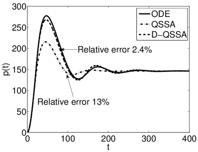
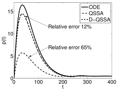
Figure 1: Numerical solutions $p(t)$, ${\hat{p}}(t)$, and ${\tilde{p}}(t)$ of ODE system $(\ref{eq:exODE_d})$–$(\ref{eq:exODE_p})$, QSSA system $(\ref{eq:exQSSA_D})$–$(\ref{eq:exQSSA_P})$, and D-QSSA system $(\ref{eq:exD-QSSA_D})$–$(\ref{eq:exD-QSSA_P})$. Left panel corresponds to parameter values $(\ref{eq:param1})$, the right panel to $(\ref{eq:param2})$.

Figure 1 (left) presents numerically computed values of $p(t)$, ${\hat{p}}(t)$, and ${\tilde{p}}(t)$ for $t\in[0,T]$ as given by $(\ref{eq:exODE_d})$–$(\ref{eq:exODE_p})$, $(\ref{eq:exQSSA_D})$–$(\ref{eq:exQSSA_P})$, and $(\ref{eq:exD-QSSA_D})$–$(\ref{eq:exD-QSSA_P})$, respectively. We observe that the approximation provided by the D-QSSA is much more accurate than the standard quasi-steady state approximation. Quantitatively, the $L^{2}$ relative error of the quasi-steady state solution ${\hat{p}}$ is approximately 13 %, while the relative error of the D-QSSA solution is approximately 2.4 %. To be rigorous,

$$\frac{\|p-{\hat{p}}\|_{L^{2}(0,T)}}{\|p\|_{L^{2}(0,T)}}\doteq 0.13,\quad\textrm{and}\quad\frac{\|p-{\tilde{p}}\|_{L^{2}(0,T)}}{\|p\|_{L^{2}(0,T)}}\doteq 0.024.$$

To show the quality of the QSSA and D-QSSA approximations also in different parameter regimes, we change the values of parameters $\gamma$ and $\gamma_{-1}$ to

$$\gamma=10\quad\textrm{and}\quad\gamma_{-1}=10^{-4}$$ (44)

and keep the other parameters the same as in $(\ref{eq:param1})$. This new choice of $\gamma$ and $\gamma_{-1}$ corresponds to $p_{0}=(\gamma_{-1}/\gamma)^{1/n}=10$. Figure 1 (right) shows the numerical solutions for parameter values $(\ref{eq:param2})$. In this case the relative error of the quasi-steady state solution is approximately 65 % and the error of the D-QSSA is approximately 12 %.

For completeness, Table 1 presents relative errors of all three variables in the system for both sets of parameters $(\ref{eq:param1})$ and $(\ref{eq:param2})$. This table confirms that the D-QSSA provides a considerably more accurate approximation than the QSSA for all variables in the system.

Parameters $(\ref{eq:param1})$ Parameters $(\ref{eq:param2})$ $D$ $m$ $p$ $D$ $m$ $p$ relative error QSSA 32 % 18 % 13 % 77 % 65 % 65 % relative error D-QSSA 12 % 3.6 % 2.4 % 28 % 12 % 12 %

Table 1: Relative errors of QSSA and D-QSSA for all variables of the system and for both sets of parameters.

The a priori error estimate $(\ref{eq:errest})$ provides a guaranteed bound on the error. It is accurate if the function $g(t)$ is close to constant and bounded well away from zero. However, in general it can overestimate the true error considerably, especially if the function $g(t)$ varies significantly or if it’s value is close to zero. The current example has both of these unfavourable properties. The quantities in $(\ref{eq:errest})$ are $\varepsilon=\gamma_{-1}$, $M=\gamma_{-1}+\gamma\max_{[0,T]}|p|^{n}$, $f^{\prime}=f^{\prime\prime}=0$, and $x^{0}=D(0)=1$. Using, for illustration, parameter values $(\ref{eq:param1})$ and estimate $\tilde{p}(t)\leq 300$, the error bound $(\ref{eq:errest})$ yields

$$|D(t)-\widetilde{D}(t)|\leq 1.99+2\exp(-0.02t),$$

while the true error is at most 0.32 and it does not exceed 0.05 for $t>50$. Nevertheless, this shows that the D-QSSA can provide accurate results even if the error estimate $(\ref{eq:errest})$ does not predict so.

We have also tested the influence of the last term in equation $(\ref{eq:exD-QSSA_P})$. The reason is that removing this term corresponds to the situation when we first reduce the system by the standard QSSA and then add the delay. We have found that the influence of this term on the solution is very minor. Solutions with and without this term almost coincide. This is expected if the delay is small, because then the quantity evaluated at the current time and at the delayed time differ only slightly and the term resulting from the time delay is close to zero and be neglected. This means that the application of the D-QSSA to general systems of the form described in Section 4 can be in these cases simplified. The system can be reduced by the standard QSSA first and then the delays can be added.

Parameter values $(\ref{eq:param1})$ and $(\ref{eq:param2})$ have been chosen to show the potential of the D-QSSA technique. In general, if we increase $\gamma_{-1}$ and correspondingly decrease $\gamma$ to keep the ratio $\gamma_{-1}/\gamma=p_{0}^{n}$ constant, then the delay $\tau(t)$ given in $(\ref{eq:exD-QSSA_D})$ attains smaller values, because $\tau(t)\leq 1/\gamma_{-1}$. Eventually, it is so small that the D-QSSA and QSSA approximations practically coincide. This is the situation when the two time scales in the system are well separated and both approaches provide very accurate approximation. However, in numerical tests we performed in this regime, the D-QSSA was always more accurate than the QSSA. On the other hand, if we decrease $\gamma_{-1}$ and increase $\gamma$ to keep the ratio $\gamma_{-1}/\gamma=p_{0}^{n}$ constant, then the delay $\tau(t)$ attains high values and the D-QSSA becomes very inaccurate. However, this is the situation when the time scales are not well separated and the standard QSSA is not accurate either. This behaviour of the D-QSSA is well explained by the dependence of the error estimate $(\ref{eq:errest})$ on $\varepsilon$.

Finally, we note that all these results were achieved with the delay as defined in $(\ref{eq:exD-QSSA_D})$. This delay is state dependent, because it depends on the value ${\tilde{p}}(t)$. This might be a hindrance and therefore we have tried to replace the state dependent delay by a constant delay. Based on experimental fitting to the system $(\ref{eq:exODE_D})$–$(\ref{eq:exODE_P})$, we have found that even a constant delay can provide very accurate results. Choosing $\tau(t)=6$ for parameter set $(\ref{eq:param1})$ and $\tau(t)=0.89$ for parameters $(\ref{eq:param2})$, we achieve relative errors in $p$ of approximately 1 %. However, the accuracy of these approximations is quite sensitive to the value of the delay and so far it is not clear how to determine the optimal constant value of the delay.

6 Cell cycle model

The D-QSSA approach seems to be especially suitable for oscillating systems. In this section, we provide an example of the application of the D-QSSA to a cell-cycle model and we will see that the standard QSSA destroys the oscillations, but the reduction by the D-QSSA keeps them. In addition, we use this example to show the application of the D-QSSA in a recurrent manner as was mentioned in Section 4. Further, we will use this example to illustrate the potential of simplifying the time varying delays to a constant delays and compare various possible choices of the constant delay.

6.1 System reduction

We consider the cell cycle model from [8]:

$$\frac{\mathrm{d}}{\mathrm{d}t}C(t) =\alpha_{1}-\beta_{1}C(t)\frac{A^{n_{1}}(t)}{K_{1}^{n_{1}}+A^{n_{1}}(t)},$$

$$\frac{\mathrm{d}}{\mathrm{d}t}P(t) =\alpha_{2}(1-P(t))\frac{C^{n_{2}}(t)}{K_{2}^{n_{2}}+C^{n_{2}}(t)}-\beta_{2}P(t),$$ (45)

$$\frac{\mathrm{d}}{\mathrm{d}t}A(t) =\alpha_{3}(1-A(t))\frac{P^{n_{3}}(t)}{K_{3}^{n_{3}}+P^{n_{3}}(t)}-\beta_{3}A(t)$$

with parameter values $\alpha_{1}=0.1,\ \alpha_{2}=\alpha_{3}=3,\ \beta_{1}=3,\ \beta_{2}=\beta_{3}=1,\ K_{1}=K_{2}=K_{3}=0.5,\ n_{1}=n_{2}=n_{3}=8.$ In this model, $C$, $P$, and $A$ correspond to the cyclin-dependent protein kinase (CDK1), the polo-like kinase 1 (Plk1), and the anaphase-promoting complex (APC), respectively. We solve this system numerically, using the zero initial condition. Figure 2 shows the solution component $C(t)$ as the solid line. Clearly, the system exhibits sustained oscillations.

All three variables in system $(\ref{eq:ccorig})$ vary on a comparable timescale and, thus, a straightforward application of the QSSA to one of these variables can hardly be successful. However, just for further comparison, we first reduce the system by the standard QSSA for $P$:

$$\frac{\mathrm{d}}{\mathrm{d}t}C(t) =\alpha_{1}-\beta_{1}C(t)\frac{A^{n_{1}}(t)}{K_{1}^{n_{1}}+A^{n_{1}}(t)},$$

$$\frac{\mathrm{d}}{\mathrm{d}t}A(t) =\alpha_{3}(1-A(t))\frac{P_{\mathrm{s}}^{n_{3}}(t)}{K_{3}^{n_{3}}+P_{\mathrm{s}}^{n_{3}}(t)}-\beta_{3}A(t),$$ (46)

$$P_{\mathrm{s}}(t) =\left[1+\frac{\beta_{2}}{\alpha_{2}}\left(1+\frac{K_{2}^{n_{2}}}{C^{n_{2}}(t)}\right)\right]^{-1}.$$

The solution component $C(t)$ of this reduced system is presented in Figure 2 by the dotted line. The QSSA for $P$ destroyed the oscillations.

Similarly, we now apply the D-QSSA to $P$. The ODE for $P$ in $(\ref{eq:ccorig})$, can be easily expressed in the form $(\ref{eq:ode1})$ and the D-QSSA can be formally applied. We obtain a system of two differential equations with a delay:

$$\frac{\mathrm{d}}{\mathrm{d}t}C(t) =\alpha_{1}-\beta_{1}C(t)\frac{A^{n_{1}}(t)}{K_{1}^{n_{1}}+A^{n_{1}}(t)},$$

$$\frac{\mathrm{d}}{\mathrm{d}t}A(t) =\alpha_{3}(1-A(t))\frac{P_{\mathrm{sd}}^{n_{3}}(t)}{K_{3}^{n_{3}}+P_{\mathrm{sd}}^{n_{3}}(t)}-\beta_{3}A(t),$$ (47)

$$P_{\mathrm{sd}}(t) =\left[1+\frac{\beta_{2}}{\alpha_{2}}\left(1+\frac{K_{2}^{n_{2}}}{C^{n_{2}}(t-\tau)}\right)\right]^{-1},\quad\tau=\left[\alpha_{2}\frac{C^{n_{2}}(t)}{K_{2}^{n_{2}}+C^{n_{2}}(t)}+\beta_{2}\right]^{-1}.$$

As the initial history we extend the zero values for $t=0$ to all $t<0$ and solve this delay system numerically. The dashed line in Figure 2 shows the solution component $C(t)$. In this case, we do observe sustained oscillations, although their period and amplitude do not accurately correspond to the original system $(\ref{eq:ccorig})$.

Finally, we will illustrate the capabilities of the D-QSSA approach and reduce the system even more. This is an example of the recurrent application of the D-QSSA, as was mentioned in Section 4. We simply consider system $(\ref{eq:ccDQSSA})$, where the variable $P$ is approximated by the D-QSSA, and apply the D-QSSA to $A$. The delay differential equation for $A$ in $(\ref{eq:ccDQSSA})$ can be formally written in the form $(\ref{eq:ode1})$ and the D-QSSA can be formally used. The result is a single differential equation with two delays:

$$\frac{\mathrm{d}}{\mathrm{d}t}C(t) =\alpha_{1}-\beta_{1}C(t)\frac{A_{\mathrm{sd}}^{n_{1}}(t)}{K_{1}^{n_{1}}+A_{\mathrm{sd}}^{n_{1}}(t)},$$

$$A_{\mathrm{sd}}(t) =\left[1+\frac{\beta_{3}}{\alpha_{3}}\left(1+\frac{K_{3}^{n_{3}}}{P_{\mathrm{sd}}^{n_{3}}(t-\tau_{2})}\right)\right]^{-1},\quad\tau_{2}=\left[\alpha_{3}\frac{P_{\mathrm{sd}}^{n_{3}}(t)}{K_{3}^{n_{3}}+P_{\mathrm{sd}}^{n_{3}}(t)}+\beta_{3}\right]^{-1},$$ (48)

$$P_{\mathrm{sd}}(t) =\left[1+\frac{\beta_{2}}{\alpha_{2}}\left(1+\frac{K_{2}^{n_{2}}}{C^{n_{2}}(t-\tau_{1})}\right)\right]^{-1},\quad\tau_{1}=\left[\alpha_{2}\frac{C^{n_{2}}(t)}{K_{2}^{n_{2}}+C^{n_{2}}(t)}+\beta_{2}\right]^{-1}.$$

We initialize the history in the same way as above and solve this delay equation numerically. The dash-dot line in Figure 2 shows the solution. Clearly, even the recurrent application of the D-QSSA yields a qualitatively correct approximation, which still oscillates.

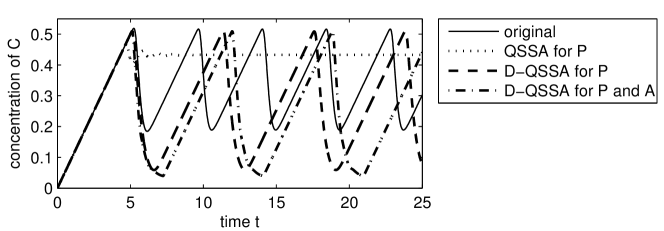
Figure 2: Solution of the original system $(\ref{eq:ccorig})$ (solid line), system reduced by the standard QSSA for $P$ $(\ref{eq:ccQSSA})$ (dotted line), system reduced by the D-QSSA for $P$ $(\ref{eq:ccDQSSA})$ (dashed line) and system reduced by the D-QSSA for both $P$ and $A$ $(\ref{eq:ccDQSSA2})$ (dash-dot line).

6.2 Effects of constant delays

As we have already mentioned, the time varying delays can be replaced by constant delays. If the constant delay is suitably chosen, the quality of the approximation can even increase. However, a suitable value for the delay is difficult to find. Here, we derive several possibilities for choosing the constant delay based on knowledge of the solution of the original system $(\ref{eq:ccorig})$. Moreover, the quality of the resulting approximations has to be assessed using again the solution of the original problem. It is not clear how to find a suitable value of the constant delay a priori, i.e. without knowledge of the original solution.

All equations in system $(\ref{eq:ccorig})$ can be formally written in the form $(\ref{eq:ode1})$. For a given equation, the delay is formally given as $\tau(t)=1/g(t)$, where $g(t)$ depends on the other components of the system. Thus, if we have the solution of this system, we know the time evolution of the time varying delay. From this evolution, we can derive constant delays in several ways. Natural choices are the minima, maxima and mean values of $\tau(t)$ over the range of $t$.

Figure 3 shows the results for the system of two differential equations $(\ref{eq:ccDQSSA})$ with a delay. We can compare the solution of the original system with the reduced systems, where the constant delay is chosen as the minimal, mean and maximal value of $\tau(t)$. The values are approximately $0.37$, $0.73$, and $1.00$, respectively. We observe that the differences among these three possibilities are relatively high and the minimal delay yields the most accurate results out of these three options. However, choosing an ad hoc value 0.3 for the delay yields even better agreement with the solution of the original problem.

Figure 4 shows similar results for the differential equation $(\ref{eq:ccDQSSA2})$ with two delays. We choose both delays as the minimal, mean, and maximal values. The delay $\tau_{1}$ applies to the variable $P$ and as such it has the same values as above, i.e. $0.37$, $0.73$, and $1.00$, respectively. The values of $\tau_{2}$ are approximately $0.32$, $0.72$, and $1.00$. Again, the minima provide the best results out of these three options. However, the ad hoc values $\tau_{1}=0.3$ and $\tau_{2}=0.28$ yield an even better approximation.

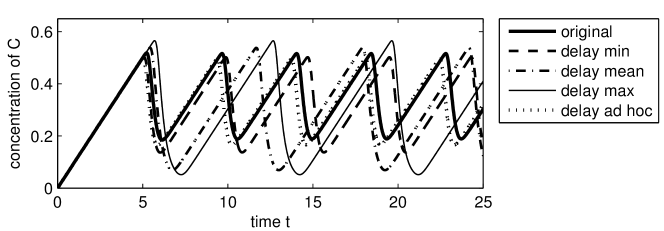
Figure 3: The thick solid line indicates the solution of the original system $(\ref{eq:ccorig})$. The remaining lines correspond to the system $(\ref{eq:ccDQSSA})$ of two differential equations with various constant values of the delay: minimal (dashed), mean (dash-dot), maximal (thin solid), and ad hoc value (dotted).

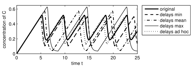
Figure 4: The thick solid line indicates the solution of the original system $(\ref{eq:ccorig})$. The remaining lines correspond to the differential equation $(\ref{eq:ccDQSSA2})$ with various constant values of the two delays. Both these delays are chosen as the minimal (dashed), the mean (dash-dot), the maximal (thin solid), and the ad hoc value (dotted).

In order to quantify the accuracy of various choices of the delays we present Table 2, where we provide relative errors in the period and amplitude of the quantity $C$ with respect to the solution of the original system $(\ref{eq:ccorig})$. The relative errors are expressed in percent and we observe that the choice of the delay has a significant influence on the accuracy. In this case, the automatic choice of the time-dependent delay yields roughly as accurate results as the mean delay computed from the solution of the original system. However, more accurate results are obtained by choosing the minimal delay, but even this choice is far from optimal, as we can see from the ad hoc choice of the delay.

Error in period/amplitude (%)	$\tau(t)$	$\min\tau(t)$	$\operatorname{mean}\tau(t)$	$\max\tau(t)$	ad hoc
two delay equations $(\ref{eq:ccDQSSA})$	42/37	10/11	42/43	59/57	0.5/0.3
one delay equation $(\ref{eq:ccDQSSA2})$	57/43	10/20	60/62	88/81	0.3/10

Table 2: Relative errors in the period and amplitude of $C$ expressed in percent and computed with respect to the solution of the original system $(\ref{eq:ccorig})$. Columns correspond to the time-dependent delay $(\ref{eq:D-QSSA})$, minimal, mean, maximal, and ad hoc values of the delays, respectively.

7 Discussion and conclusions

In this paper, we present the technique of D-QSSA, prove a corresponding error estimate, and analyse how it approximates the invariant manifold. The technique is well justified for equations of the form $(\ref{eq:ode1})$. We also show explicit application of the D-QSSA to a general mass action model of a general chemical system. However, the D-QSSA can be applied only if assumptions A1–A3 are satisfied. Assumption A1 means that the stoichiometric coefficients of the fast chemical species on the reactant side of the chemical equation cannot be greater than one, unless the species is a catalyst. This is not as severe a restriction as it may first look, because many biochemical reactions are of this type and, moreover, the assumption concerns fast species only.

Assumption A2 requires positivity of functions $g_{j}(t)$ in the equations for the fast species. This is a technical assumption whose validity can be guaranteed from the stoichiometry and rate constants of the chemical system.

Assumption A3 means that the fast variables are independent in the sense that reactants of all reactions, where a fast species is either produced or consumed, do not involve any other fast species. This tends to be satisfied in biochemical systems if the fast species correspond to genes, because genes do not directly influence each other. Moreover, this assumption is not fundamental, due to the possibility of recurrent application of D-QSSA (see Section 4 and the example in Section 6).

To summarise, these assumptions are not too restrictive and make the technique of D-QSSA applicable to the majority of mass action models of biochemical systems.

The main idea of the D-QSSA is the introduction of a time delay to improve accuracy. The standard QSSA ignores the time needed by fast variables to reach their steady states. This may result in considerable errors. The D-QSSA compensates for this time delay and improves the accuracy of the approximation. In the example presented in Section 5, the D-QSSA exhibits more than five times smaller error in comparison with the standard QSSA.

In comparison with the standard QSSA, the D-QSSA seems to be especially useful for oscillating systems. The standard QSSA usually causes considerable errors in both the period and amplitude of oscillations [33]. The D-QSSA enables this error to be reduced substantially. In [32] we have successfully applied the technique of D-QSSA to a system for modelling circadian rhythms [33]. This system is described by nine ODEs and it can be reduced to two. The standard QSSA yields roughly 30 % error in the period, while the D-QSSA approach approximates the period with errors of about 1–2 %.

The D-QSSA can be applied even in cases when the standard QSSA destroys the oscillations completely. In Section 6, we provide an example of such a successful application of the D-QSSA. The original cell-cycle model consists of three ODEs and it has been reduced to one delay differential equation which yields sustained oscillations. This indicates that the oscillations in this cell-cycle model are driven by delayed negative feedback.

The D-QSSA and the proposed choice of the delays are in agreement with the conclusions of [27] where systems with constant coefficient $g$ are considered. The delays derived in [27], by a careful analysis of two specific examples, are identical to the delays obtained by the D-QSSA.

The case of varying delays may be problematic for both numerical solution and subsequent analysis. However, numerical experiments both in this paper and in [32] show that a constant approximation of the varying delay yields accurate results as well. Nevertheless, the quality of this approximation is quite sensitive to the value of the constant delay and its optimal choice is not clear. To make the constant delay approach practical, subsequent research is necessary.

The essential first step for both the standard QSSA and the D-QSSA is the identification of the fast variables. However, in some systems none of the variables can be considered as fast, while a suitable combination can. Reference [17] shows how to identify such combinations and how to apply the QSSA to these variables. The technique of the D-QSSA can be applied in these cases as well and we will investigate this possibility in future research.

In chemical systems, the delay in the D-QSSA depends also on the rate constants of the chemical reactions involved. Thus, the technique of the D-QSSA can be used in situations where complex chemical processes are modelled by a simple reaction with a time delay [1, 20, 29], to determine and analyse how the delay actually depends on various parameters of the system. This promises new insight and understanding of models with time delays. We plan, in future work, to apply the D-QSSA to a detailed chemical model of transcription [28, 29] to derive and analyse the dependence of the transcriptional delay on the rates of the elementary chemical reactions which comprise the process.

References

- [1] Bernard, S., Čajavec, B., Pujo-Menjouet, L., Mackey, M.C., Herzel H. (2006). Modelling transcriptional feedback loops: the role of Gro/TLE1 in Hes1 oscillations. Phil. Trans. R. Soc. A 364, 1155–1170.
- [2] Bodenstein, M. (1913). Eine Theorie der photochemischen Reaktionsgeschwindigkeiten. Zeitschrift für physikalische Chemie 85, 329–397.
- [3] Borghans, J.A.M., de Boer, R.J., Segel, L.A. (1996). Extending the quasi-steady state approximation by changing variables. Bulletin of Mathematical Biology 58(1), 43–63.
- [4] Bratsun, D., Volfson, D., Tsimring, L.S., Hasty, J. (2005). Delay-induced stochastic oscillations in gene regulation. Proc. Natl. Acad. Sci. U.S.A. 102(41), 14593–14598.
- [5] Briggs, G.E., Haldane, J.B.S. (1925). A note on the kinetics of enzyme action. Biochem. J. 19(2), 338–339.
- [6] Chapman, D.L., Underhill, L.K. (1913). The interaction of chlorine and hydrogen. The influence of mass. Journal of the Chemical Society, Transactions 103, 496–508.
- [7] Chellaboina, V., Bhat, S., Haddad, M.M., Bernstein, D.S. (2009). Modeling and analysis of mass-action kinetics. IEEE Control Systems Magazine 29(4), 60–78.
- [8] Ferrell Jr, J.E., Tsai, T.Y.C., Yang, Q. (2011). Modeling the cell cycle: why do certain circuits oscillate? Cell, 144(6), 874–885.
- [9] Fraser, S.J. (1988). The steady state and equilibrium approximations: A geometrical picture. J. Chem. Phys. 88(8), 4732–4738.
- [10] Gear, C.W., Kevrekidis, I.G. (2005). Constraint-defined manifolds: a legacy code approach to low-dimensional computation. Journal of Scientific Computing 25(1), 17–28.
- [11] Gorban, A.N., Karlin, I.V. (2003). Method of invariant manifold for chemical kinetics. Chemical Engineering Science 58(21), 4751–4768.
- [12] Gorban, A.N., Karlin, I.V., Zinovyev, A.Y. (2004). Constructive methods of invariant manifolds for kinetic problems. Physics Reports 396, 197–403.
- [13] Hirata, H., Yoshiura, S., Ohtsuka, T., Bessho, Y., Harada, T., Yoshikawa, K., Kageyama, R. (2002). Oscillatory expression of the bHLH factor Hes1 regulated by a negative feedback loop. Science 298, 840–843.
- [14] F. Horn, R. Jackson (1972). General mass action kinetics. Arch. Rational Mech. Anal. 47(2), 81–116.
- [15] Lam, S.H. (1993). Using CSP to understand complex chemical kinetics. Combust. Sci. Technol. 89(5–6), 375–404.
- [16] Lebiedz, D. (2004). Computing minimal entropy production trajectories: An approach to model reduction in chemical kinetics. J. Chem. Phys. 120(15), 6890–6897.
- [17] Lee, C.H., Othmer, H.G. (2010). A multi-time-scale analysis of chemical reaction networks: I. Deterministic systems. J. Math. Biol. 60, 387–450.
- [18] Leitold, A., Hangos, K.M., Tuza, Z. (2002). Structure simplification of dynamic process models. Journal of Process Control 12(1), 69–83.
- [19] Michaelis, L., Menten, M.L. (1913). Die Kinetik der Invertinwirkung. Biochem. Z. 49, 333–369.
- [20] Monk, N.A.M. (2003). Oscillatory expression of Hes1, p53, and NF-B driven by transcriptional time delays. Current Biology 13(16), 1409–1413.
- [21] Nguyen, A.H., Fraser, S.J. (1989). Geometrical picture of reaction in enzyme kinetics. J. Chem. Phys. 91(1), 186–193.
- [22] Okino, M.S., Mavrovouniotis, M.L. (1998). Simplification of mathematical models of chemical reaction systems. Chemical Reviews 98(2), 391–408.
- [23] Prestel, A., Delzell, C.N. (2001). Positive polynomials. Springer-Verlag, Berlin.
- [24] Radulescu, O., Gorban, A., Zinovyev, A., Lilienbaum, A. (2008). Robust simplifications of multiscale biochemical networks. BMC Systems Biology 2:86, 25p.
- [25] Roussel, M.R. (1996). The use of delay differential equations in chemical kinetics. Journal of Physical Chemistry 100(20), 8323–8330.
- [26] Roussel, M.R., Fraser, S.J. (1991). On the geometry of transient relaxation. J. Chem. Phys. 94(11), 7106–7113.
- [27] Roussel, C.J., Roussel, M.R. (2001). Delay-differential equations and the model equivalence problem in chemical kinetics. Physics in Canada 57(2), 114–120.
- [28] Roussel, M.R., Zhu, R. (2006). Stochastic kinetics description of a simple transcription model. Bull. Math. Biol. 68(7), 1681–1713.
- [29] Roussel, M.R., Zhu, R. (2006). Validation of an algorithm for delay stochastic simulation of transcription and translation in prokaryotic gene expression. Physical Biology 3(4), 274–284.
- [30] Segel, L.A., Slemrod, M. (1989). The quasi-steady-state assumption: a case study in perturbation. SIAM Review 31(3), 446–477.
- [31] Turányi, T., Tomlin, A. S., Pilling, M.J. (1993). On the error of the quasi-steady-state approximation. J. Phys. Chem. 97, 163–172.
- [32] Vejchodský, T. (2013). Accurate reduction of a model of circadian rhythms by delayed quasi steady state assumptions. Preprint arXiv:1312.2825, to appear in Mathematica Bohemica.
- [33] Vilar, J.M.G., Kueh, H.Y., Barkai, N., Leibler, S. (2002). Mechanisms of noise-resistance in genetic oscillators. PNAS 99(9), 5988–5992.
- [34] Zagaris, A., Kaper, H.G., Kaper, T.J. (2004). Analysis of the computational singular perturbation reduction method for chemical kinetics. Journal of Nonlinear Science 14(1), 59–91.