Temperature Structure of the Intra-Cluster Medium from SPH and AMR simulations

Abstract

Analyses of cosmological hydrodynamic simulations of galaxy clusters suggest that X-ray masses can be underestimated by 10%–30%. The largest bias originates by both violation of hydrostatic equilibrium (HE) and an additional temperature bias caused by inhomogeneities in the X-ray emitting intra-cluster medium (ICM). To elucidate on this large dispersion among theoretical predictions, we evaluate the degree of temperature structures in cluster sets simulated either with smoothed-particle-hydrodynamics (SPH) and adaptive-mesh-refinement (AMR) codes. We find that the SPH simulations produce larger temperature variations connected to the persistence of both substructures and their stripped cold gas. This difference is more evident in nonradiative simulations, while it is reduced in the presence of radiative cooling. We also find that the temperature variation in radiative cluster simulations is generally in agreement with the observed one in the central regions of clusters. Around $R_{500}$ the temperature inhomogeneities of the SPH simulations can generate twice the typical HE mass bias of the AMR sample. We emphasize that a detailed understanding of the physical processes responsible for the complex thermal structure in ICM requires improved resolution and high sensitivity observations in order to extend the analysis to higher temperature systems and larger cluster-centric radii.

1 Introduction

A number of independent analyses on cosmological hydrodynamic simulations of galaxy clusters consistently show that hydrostatic equilibrium (HE) masses underestimate true masses by 10%–30%, the exact value depending on the physics of the intracluster medium (ICM), the hydrodynamic scheme, the radius within which the mass is measured, and the dynamical state of the clusters (Rasia et al. 2004; Piffaretti & Valdarnini 2008; Jeltema et al. 2008; Ameglio et al. 2009; Lau et al. 2009; Nelson et al. 2012; Sembolini et al. 2013; Ettori et al. 2013)

Rasia et al. (2012, hereafter R12), using synthetic Chandra observations of a set of massive clusters simulated with the smoothed-particle hydrodynamics (SPH) GADGET code, found ICM temperature inhomogeneities to be responsible for 10%–15% mass bias, which adds to a comparable bias associated with the violation of HE (see also Rasia et al., 2006). On the other hand, no significant contribution to the mass bias associated with ICM thermal inhomogeneities was found by Nagai et al. (2007a, b, hereafter N07), who analyzed simulations from the Eulerian adaptive-mesh refinement (AMR) code ART, or by Meneghetti et al. (2010, hereafter M10), who investigated SPH simulations including thermal conduction. Temperature perturbations of the N07 sample are, indeed, verified to provide a negligible contribution (less than 5% within $R_{500}$) to X-ray temperature bias (Khedekar et al., 2013). At the same time, the presence of thermal conduction tends to homogenize the temperature of the medium especially in massive systems (Dolag et al., 2004).

A theoretical clarification of the mismatch on the X-ray mass bias is quite timely after the reported conflict between the constraints on cosmological parameters derived from primary cosmic-microwave-background anisotropies measured by Planck and cluster number counts (Planck Collaboration et al., 2013). A suggested solution for the reconciliation of the two sets of parameters seeks a bias on the X-ray masses as large as 40% (see also von der Linden et al., 2014). The observational evaluation of such a bias is often done by comparing the masses derived from X-ray with those estimated through gravitational lensing, believed to illustrate the true masses. Simulations, however, indicate that even the gravitational lensing technique could be biased (Becker & Kravtsov, 2011, M10; R12) because of the triaxiality of the cluster potential well or the presence of substructures located either within the cluster or along the line of sight. These complications affect individual observations and, therefore, generate a significant scatter around the true mass. As a matter of fact, as of today no clear convergence has been reached on the observational ratio between X-ray and gravitational lensing masses (Zhang et al., 2008; Mahdavi et al., 2008; Zhang et al., 2010; Jee et al., 2011; Foëx et al., 2012; Mahdavi et al., 2013; von der Linden et al., 2014; Israel et al., 2014).

Because of the difficulties of establishing the amplitude of the X-ray mass bias from observations, the interpretation of the aforementioned theoretical disagreement can be done only by systematically analyzing the temperature inhomogeneities present in the three samples of N07, M10, and R12. In this work, we group the simulated clusters into two sets generically labeled the SPH set and the AMR set (see Section 2). Despite this naming choice, we would like to stress that our analysis does not aim to be a code-comparison project for which other conditions (such as common initial conditions) need to be met (e.g. Frenk et al., 1999; O’Shea et al., 2005; Valdarnini, 2012; Power et al., 2014).

After the characterization of the inhomogeneities in the samples we will investigate how our simulated data relate to observations. Both SPH and AMR simulations have already been shown to reproduce the observed temperature profiles, at least outside the cluster core regions (see reviews by Borgani & Kravtsov, 2011; Reiprich et al., 2013, and references therein). However, no detailed comparison has been carried out so far for the small-scale ICM temperature structure mostly because of a lack of observational measurements. Fluctuations in density and temperature have been measured only in a few nearby, dynamically disturbed clusters (Bourdin & Mazzotta, 2008; Bautz et al., 2009; Zhang et al., 2009; Gu et al., 2009; Bourdin et al., 2011; Churazov et al., 2012; Bourdin et al., 2013; Rossetti et al., 2013; Schenck et al., 2014). Just recently, Frank et al. (2013) (hereafter F13) measured the temperature distribution in the central region (within $R_{2500}$) of 62 galaxy clusters identified in the HIghest X-ray FLUx Galaxy Cluster Sample (HIFLUGCS Reiprich & Böhringer, 2002). F13 analyzed the X-ray Multi-Mirror (XMM-Newton) observations by adopting the smoothed-particle interference technique (Peterson et al., 2007). For each cluster, they built the emission-measured temperature distribution, calculated its median and dispersion.

Simulations are described in Section 2. The analysis is divided into three parts. First, we measure the temperature variation and interpret the results by comparing the performances of the SPH and AMR codes (Section 3). Second, we investigate how temperature fluctuations are connected with density fluctuations (Section 4). Finally, we compare the radiative simulations with the observational data of F13 (Section 5). We discuss the impact that temperature inhomogeneities have on the hydrostatic mass estimates in Section  6 and outline our conclusions in Section 7.

2 Simulations

In this work, we analyze the original cluster samples simulated with the SPH technique from which the subsamples of R12 and M10 were extracted. In addition, we study four different implementations of the ICM physics. At the same time, we add about 85 clusters taken from Nelson et al. 2014 (hereafter N14) to the 16 objects of N07. The new set is carried out with the same AMR code of N07 with the implementation of nonradiative physics.

Both the SPH and AMR sets assume a flat $\Lambda$-cold-dark-matter model with small differences in the choice of cosmological parameters. The small changes are not expected to affect our results. The SPH, N07, N14 simulations, respectively, adopt: $\Omega_{\rm M}=$ 0.24, 0.3, 0.27 for the matter density parameter; $\Omega_{\rm bar}=$ 0.040, 0.043, 0.047 for the baryon density; $H_{0}$ = 72, 70, 70 km s^-1 Mpc^-1 for the Hubble constant at redshift zero; and $\sigma_{8}=$ 0.8, 0.9, 0.82 for the normalization of the power spectrum on a scale of 8 $h^{-1}$ Mpc.

2.1 Smoothed-Particle Hydrodynamics Sets

The largest SPH set includes halos identified within 29 Lagrangian regions selected from a low-resolution $N$-body simulation of volume equal to 1 ($h^{-1}$Gpc)³ and resimulated at high resolution (Bonafede et al., 2011). Twenty-four of these regions are centered on the most massive clusters of the parent $N$-body simulation, while the remaining are centered on group-size halos. The size of the regions is such that no low-resolution contaminant dark-matter (DM) particle is found within five virial radii from the central halo. Within all of the regions, further halos are identified leading to $\sim 160$ as the total number of objects with mass $M_{\rm vir}>3\times 10^{13}$ $h^{-1}$$M_{\odot}$. We limit this study to 49 systems with mass $M_{500}$ greater than $0.9\times 10^{14}$ $h^{-1}$$M_{\odot}$. This threshold corresponds to a mass-weighted temperature $T_{\rm MW}(<R_{500})\approx 2$ keV when using the mass–temperature relation derived by Planelles et al. (2013) and Fabjan et al. (2011).

The resimulations are carried out with the TreePM-SPH GADGET-3 code (Springel, 2005) with three different flavors for the ICM physics:

1. ${\rm NR_{SPH}}$: nonradiative physics with an entropy-conserving prescription for the SPH (Springel & Hernquist, 2002) and artificial viscosity with the viscosity delimiter described by Balsara (1995) and Steinmetz (1996)

2. ${\rm CSF_{SPH}}$: including radiative cooling, star formation, and feedback in energy and metals from supernovae. The radiative cooling, introduced as in Wiersma et al. (2009), accounts for cosmic microwave background, UV/X-ray background radiation from quasars and galaxies (Haardt & Madau, 2001), and metal cooling typical of an optically thin gas in photoionization equilibrium (Ferland et al., 1998). The star formation and evolution is treated via multiphase particles (Springel & Hernquist, 2003) with a coexisting cold and hot phases. Stars are distributed assuming the initial mass function of Chabrier (2003) and evolve following the recipes of Padovani & Matteucci (1993). The kinetic feedback (Springel & Hernquist, 2003) released from the explosion of supernovae was implemented assuming velocity of the winds equal to $v_{w}=500$ s^-1 km. The simulated clusters analyzed by R12 are a subsample of this set.

3. ${\rm AGN_{SPH}}$: similar to the previous physics but also adding the feedback from active galactic nuclei (AGNs) resulting from gas accretion onto super-massive black holes (SMBH; see Ragone-Figueroa et al., 2013). The numerical scheme is largely based on that originally proposed by Springel et al. (2005). It follows the evolution of SMBH particles whose dynamics are controlled only by gravity and whose mass grows by accretion from the surrounding gas or mergers with other SMBHs. The accretion produces radiative energy with an efficiency of 0.2, of which 20% is thermally given to the gas particles in the vicinity of the SMBH. Ragone-Figueroa et al. (2013) find that the original method by Springel et al. (2005) needs some modifications concerning: (1) the way SMBHs act as sinks of gas, (2) the strategy to place the SMBHs at the center of the hosting galaxy, and (3) how the radiative energy produced by accretion is returned to the interstellar medium. These changes are essential in order to adapt the numerical scheme to the moderate resolution of cosmological simulations as well as to produce a sensitive coupling with the multiphase model adopted to treat star formation.

Masses of dark matter and gas particles are $m_{\rm dm}=8.47\times 10^{8}$ $h^{-1}M_{\odot}$ and $m_{\rm gas}=1.53\times 10^{8}$ $h^{-1}M_{\odot}$, respectively. The adopted Plummer-equivalent softening length for gravitational force is fixed to $\epsilon=5$ $h^{-1}$ kpc in physical units below redshift $z=2$, and it is set to the same value in comoving units at higher redshift. The minimum SPH smoothing length is $0.5\times\epsilon$.

In order to assess the effect of thermal conduction in SPH simulations, we further analyze the nine main halos from Dolag et al. (2009) from which the sample of M10 was extracted. The choices of particle mass and softening are similar to the previous sets.

1. ${\rm TH.C_{SPH}}$: among the objects listed in Table 2 of Dolag et al. (2009), we specifically consider those labeled with the letter a. The simulation sets studied here are csf and csfc. The former is equivalent to the treatment of the ${\rm CSF_{SPH}}$ set, and the latter includes the effect of thermal conduction (Jubelgas et al., 2004; Dolag et al., 2004), characterized by a conductivity fixed to one-third the Spitzer conductivity of a fully ionized unmagnetized plasma.

2.2 Adaptive-mesh Refinement simulations

The AMR set includes the clusters at $z=0$ studied in N07 and N14. We refer the reader to both papers for the details of the simulations. Here we summarize their key properties. Simulations were carried out with the adaptive-refinement treeART code (Kravtsov et al., 1997; Rudd et al., 2008), a Eulerian code that uses adaptive refinement in space and time and nonadaptive refinement in mass (Klypin et al., 2001) to achieve the dynamic range necessary to resolve the cores of halos formed in self-consistent cosmological simulations.

The 16 clusters from N07 are simulated using a uniform $128^{3}$ grid and eight levels of mesh refinement in boxes of $120$ $h^{-1}$ Mpc and $80$ $h^{-1}$ Mpc as sides, corresponding to peak spatial resolution of about $3.66$ $h^{-1}$ kpc and $2.44$ $h^{-1}$ kpc, respectively. The DM particle mass inside the virial radius is $m_{\rm dm}=9.1\times 10^{8}$ $h^{-1}M_{\odot}$ and $m_{\rm dm}=2.7\times 10^{8}$ $h^{-1}M_{\odot}$ for the two box sizes, respectively, and external regions are simulated with lower mass resolution. The N07 clusters are simulated with two gas physics recipes: (1) nonradiative gas physics (${\rm NR_{AMR}}$) and (2) galaxy formation physics with metallicity-dependent radiative cooling, star formation, thermal feedback from supernovae type Ia and II, and UV heating due to cosmological ionizing background (${\rm CSF_{AMR}}$).

The cluster sample of N14 is simulated in a cosmological box of $500$ $h^{-1}$ Mpc on a side, with a uniform $512^{3}$ grid and eight levels of mesh refinement, corresponding to a maximum comoving spatial resolution of $3.8$ $h^{-1}$ kpc. We identify and select $85$ cluster-size halos with $M_{500}\geq 2\times 10^{14}$ $h^{-1}M_{\odot}$. The virial regions surrounding the selected clusters are resolved with a DM particle mass of $m_{\rm dm}=1.0\times 10^{9}$ $h^{-1}M_{\odot}$  corresponding to an effective particle number of $2048^{3}$ in the entire box, and the external regions are simulated with lower mass resolution. The clusters are simulated with nonradiative gas physics only and are used as a control sample. The larger statistics validate results from the N07 nonradiative set.

2.3 Exclusion of Cold Gas Particles.

Radiative cooling converts part of the gas from the hot and diffuse phase to a cold and dense phase, resulting in a runaway cooling that increases the amount of cooled baryons unless the process is regulated by energy feedback by stars and black holes. The gas most affected by this process is located in the central regions of the central galaxies or merging subhalos. Most of the gas in the cooled phase has sufficiently low temperature and hence does not emit in the X–ray band. However, a small fraction of it, being dense and having a temperature of order of a few $10^{6}$ K, might form bright clumps visible in soft X-ray images (Roncarelli et al., 2006; Zhuravleva et al., 2013; Vazza et al., 2013; Roncarelli et al., 2013).

Careful X-ray analysis on Chandra-like mock images requires the detection of these clumps through a wavelength algorithm (e.g. Vikhlinin et al., 1998) as done in N07 and R12 (see also Rasia et al., 2006; Ventimiglia et al., 2012; Vazza et al., 2013) and their consequent masking. To extend the observational approach to the direct study of simulated systems, other techniques, based on the density or volume of the gas elements, have been proposed in the literature. In Roncarelli et al. (2006, 2013), the densest particles of each spherical shell of constant width ($\sim 0.5\times R_{200}$) are excluded once their cumulative volume reaches 5% of the total particle volume in the shell. Zhuravleva et al. (2013) suggested cutting all cells with gas density $\rho$ that satisfies the condition $\log\rho>\log\{\rho\}+3\sigma_{10,\rho}$, where $\{\rho\}$ is the median of the density in the radial shell and $\sigma_{10,\rho}$ is analogous to the standard deviation of the log-normal distribution. R12 proposed a different approach that also takes into account the information on the temperature of the cooled gas and eliminates all gas elements with $T<3\times 10^{6}\rho^{0.25}$ where the temperature, $T$, is expressed in keV and the gas density, $\rho$, in g cm^-3. The slope of this relation is linked to the effective polytropic index of the gas, and the value of the normalization weakly depends on the cluster temperature (see Appendix A of R12) and does not vary for the samples considered in this paper. Removing gas particles (in SPH) and cells (in AMR) according to this criterion amounts to excluding less than 0.1% of the gas volume, about 10 times less than the amount selected by the other methods.

In the rest of this paper, the analysis on all radiative simulations (${\rm CSF_{SPH}}$, ${\rm AGN_{SPH}}$, TH.C_SPH, and ${\rm CSF_{AMR}}$) is performed after the exclusion of the cold gas, as done in R12. We find that this criterion in addition to more effectively removing the multiphase gas, also preserves the presence of merging small-group-size substructures. This requisite is essential to comparing our simulations to the observational data of F13, who analyzed the whole region within $R_{2500}$ without applying any masking either on substructures or on the core. No gas has, instead, been removed in the nonradiative simulation (${\rm NR_{SPH}}$ and ${\rm NR_{AMR}}$).

3 Temperature structure in simulations

3.1 Measurements of ICM Temperature

From the values of mass ($m$), density, and temperature of each gas element (particle or cell), we compute the gas mass-weighted temperature, $T_{\rm MW}$, and the spectroscopic-like temperature (Mazzotta et al., 2004; Vikhlinin, 2006), $T_{\rm SL}$, defined as

$$T=\frac{\Sigma W_{i}T_{i}}{\Sigma W_{i}}\ \ \ \ {\rm with}\ \ \ \ \ W_{i,\rm MW}=m_{i},\ \ {\rm or}\ \ \ W_{i,\rm SL}=m_{i}\rho_{i}T_{i}^{-0.75}.$$ (1)

In the above equation, the summation signs run over the gas elements belonging to three regions: the innermost is the sphere with radius $R_{2500}$ and the intermediate and outermost regions are spherical shells delimited by [$R_{2500}$, $R_{500}$] and by [$R_{500}$, $R_{200}$]. We label these regions I, M, and O, respectively.

$T_{\rm{MW}}$ has a well-defined physical meaning because it is directly related to the total thermal energy of the ICM: $E_{\rm th}\sim m\times$ $T_{\rm{MW}}$. As such, it is the temperature that should be entered into the HE mass estimate. $T_{\rm{SL}}$, on the other hand, is the temperature directly accessible to X-ray spectroscopy, and it is more sensitive to dense gas than $T_{\rm{MW}}$. In our analysis we include all particles or cells with temperature above 0.5 keV (Mazzotta et al., 2004). For a thermally uniform medium these two temperatures coincide. Any difference between them, $\Delta_{T}=$ $T_{\rm{MW}}$$-$ $T_{\rm{SL}}$$>0$, could be interpreted as a quantitative measure of inhomogeneities in the ICM thermal structure. As matter of fact, the relation $T_{\rm{SL}}$$<$ $T_{\rm{MW}}$ is verified whenever cold and dense gas is within the considered region. The opposite situation, $T_{\rm{MW}}$$<$ $T_{\rm{SL}}$, exists in the presence of a negative temperature gradient aligned with a positive mass gradient, as usually is the case in the outskirts of relaxed objects.

The dependence of $\Delta_{T}$ on $T_{\rm MW}$ for the SPH and AMR codes is shown in Figure 1. Tables 1 and  3 report the best-fit linear relations to $T_{\rm{MW}}$-$\Delta_{T}$ along with the associated intrinsic scatter $\sqrt{\chi^{2}/(N-1)}$, where $N$ is the number of clusters analyzed. The best fits are computed by minimizing the $\chi^{2}$ error statistic.

3.2 Smoothed-Particle Hydrodynamics

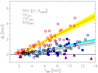
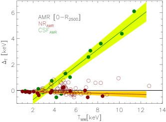
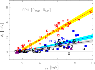
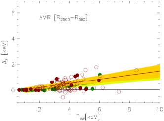
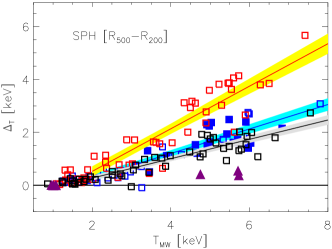
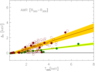
Figure 1: Temperature variation, $\Delta_{T}=$ $T_{\rm{MW}}$$-$$T_{\rm{SL}}$, vs. $T_{\rm{MW}}$ for the SPH (left panels) and AMR (right panels) simulations measured in the I (top panel), M (center panel), and O regions (bottom panel). Left panels: red, blue, and black squares correspond to ${\rm NR_{SPH}}$, ${\rm CSF_{SPH}}$, and ${\rm AGN_{SPH}}$, respectively, and purple triangles refer to ${\rm TH.C_{SPH}}$. Filled squares indicate the subset analyzed by R12. Right panels: brown and green circles correspond to ${\rm NR_{AMR}}$ and ${\rm CSF_{AMR}}$, respectively. Filled circles indicate the subset analyzed by N07. The shaded regions represent the 1$\sigma$ scatter around the best-fitting relations. For clarity, we omit the best-fit relation of the thermal conduction simulations (see Table 1).

The left panels of Figure 1 show the temperature variation, $\Delta_{T}$, measured in the SPH simulations. As a general trend, the nonradiative physics presents the largest degree of temperature variation at all radii and along the entire temperature range. ${\rm CSF_{SPH}}$ clusters behave similar to ${\rm AGN_{SPH}}$ in the innermost region but are typically above in the more external shells. ${\rm TH.C_{SPH}}$ objects are characterized by a small variation in temperature $\Delta_{T}<0.5$ keV. The differences between radiative and nonradiative simulations are expected because the cooling process preferentially removes low-entropy gas (especially that associated with central galaxies and merging substructures) from the diffuse phase. This phenomenon, combined with the heating provided by supernovae, decreases the temperature contrast between clumps and diffuse ICM. In the intermediate and outermost regions, the slope of the $T_{\rm{MW}}$$-\Delta_{T}$ relation for the CSF_SPH simulations decreases by 40–60% with respect to the NR_SPH case (Table 1).

The increase of the $T_{\rm{MW}}$$-\Delta_{T}$ slope moving outward is expected because the outskirts of the most massive systems are more severely affected by inhomogeneities generated by ongoing gas accretions along filaments. This picture is consistent with the increase of the clumpy factor with radius (Nagai & Lau, 2011; Vazza et al., 2013; Khedekar et al., 2013; Roncarelli et al., 2013). The accreting clumps are larger and survive longer in nonradiative simulations (Dolag et al., 2009), affecting more strongly the spectroscopic-like temperature without significantly influencing the mass-weighted temperature. This statement is illustrated in the left panel of Figure 2 where we show how the spectroscopic-like temperature and the mass-weighted temperature change in radiative simulations with respect to nonradiative simulations. On the other hand, the imprint of the particular feedback model (either by supernovae or by AGNs) has less impact on the calculation of both temperatures (right panel of Figure 2). Thermal conduction minimally influences small clusters but induces 50% - 100% variations in the $T_{\rm SL}$ measurements of the four most massive systems. That said, the slope of the $T_{\rm{MW}}$$-\Delta_{T}$ is still a factor of two-to-three lower than the ${\rm CSF_{SPH}}$ case.

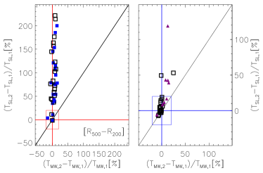
Figure 2: Difference between the two temperatures (mass-weighted and spectroscopic-like) as measured within the various SPH simulations in the O region. Left panel: the radiative cases (${\rm CSF_{SPH}}$ in blue and ${\rm AGN_{SPH}}$ in black) of the R12 sample are compared to the ${\rm NR_{SPH}}$ flavor. Right panel: ${\rm AGN_{SPH}}$ is related to ${\rm CSF_{SPH}}$ and ${\rm TH.C_{SPH}}$ is compared with the respective CSF_SPH physics. Symbols are as in Figure 1. The box in the center represents a 20% variation in both panels.

Table 1: SPH Set: Best-fit Parameters, their 1 $\sigma$ Errors, and Scatter of the Linear Relation: $\Delta_{T}$=$T_{\rm{MW}}$–$T_{\rm{SL}}$$=A+B\times$($T_{\rm{MW}}$)

all clusters
	A$\pm$ err(A)	B $\pm$ err(B)	scatter
${\rm NR_{SPH}}$, I	-0.75 $\pm$ 0.18	0.41$\pm$ 0.03	0.55
${\rm NR_{SPH}}$, M	-1.03 $\pm$ 0.18	0.67 $\pm$ 0.04	0.54
${\rm NR_{SPH}}$, O	-1.08 $\pm$ 0.19	0.80 $\pm$ 0.05	0.56
${\rm CSF_{SPH}}$, I	-0.39 $\pm$ 0.19	0.15 $\pm$ 0.023	0.53
${\rm CSF_{SPH}}$,M	-0.52 $\pm$ 0.15	0.26 $\pm$ 0.03	0.43
${\rm CSF_{SPH}}$, O	-0.65 $\pm$ 0.12	0.46 $\pm$ 0.03	0.35
${\rm AGN_{SPH}}$, I	-0.40 $\pm$ 0.12	0.14 $\pm$ 0.02	0.34
${\rm AGN_{SPH}}$,M	-0.40 $\pm$ 0.12	0.19 $\pm$ 0.02	0.36
${\rm AGN_{SPH}}$, O	-0.50 $\pm$ 0.09	0.37 $\pm$ 0.02	0.28
${\rm TH.C_{SPH}}$, I	-0.22 $\pm$ 0.11	0.0 $\pm$ 0.01	0.18
${\rm TH.C_{SPH}}$ ,M	-0.19 $\pm$ 0.13	0.12$\pm$ 0.02	0.22
${\rm TH.C_{SPH}}$, O	-0.15 $\pm$ 0.05	0.13$\pm$ 0.01	0.10
only relaxed
	A$\pm$ err(A)	B $\pm$ err(B)	scatter
${\rm NR_{SPH}}$, I	-1.01 $\pm$ 0.29	0.38$\pm$ 0.05	0.40
${\rm NR_{SPH}}$, M	-1.69 $\pm$ 0.47	0.76 $\pm$ 0.10	0.66
${\rm NR_{SPH}}$, O	-1.56 $\pm$ 0.41	0.90 $\pm$ 0.011	0.56
${\rm CSF_{SPH}}$, I	-0.37 $\pm$ 0.16	0.06 $\pm$ 0.02	0.21
${\rm CSF_{SPH}}$,M	-0.33 $\pm$ 0.27	0.17 $\pm$ 0.05	0.37
${\rm CSF_{SPH}}$, O	-1.00 $\pm$ 0.18	0.56 $\pm$ 0.05	0.24
${\rm AGN_{SPH}}$, I	-0.71 $\pm$ 0.24	0.15 $\pm$ 0.04	0.30
${\rm AGN_{SPH}}$,M	-0.17 $\pm$ 0.13	0.09 $\pm$ 0.02	0.17
${\rm AGN_{SPH}}$, O	-0.55 $\pm$ 0.20	0.37 $\pm$ 0.05	0.26

Relaxed clusters are defined in Section 6.1

The difference between the two temperatures, $T_{\rm{MW}}$ and $T_{\rm{SL}}$, measured in the ${\rm CSF_{SPH}}$ simulation is similar to those reported by Biffi et al. (2014), who analyzed about 180 massive clusters selected from the “Mare-Nostrum Multidark Simulations of Galaxy Clusters” and resimulated with the code GADGET, including the treatment of cooling, star formation, and feedback by supernovae. In that case, the average difference between $T_{\rm MW}$ and $T_{\rm SL}$ is $\sim 15\%$ when both measurements are carried out within a sphere of radius $R_{500}$. In our case, the median of the ratios varies from 6% in the I region to 14% and to 31% in the $M$ and $O$ shells. The inclusion of AGN does not change the value in the center but decreases the differences to 10% and 23% in the other two regions. As expected, major variations are present for the nonradiative simulations: the medians of the ratios are about 20% in the innermost sphere but exceed 70% elsewhere. This last value is significantly higher than the 20% predicted by the pioneering work of Mathiesen & Evrard (2001). A direct comparison is, however, arduous because (1) the cosmological models adopted there consider a higher spectrum normalization, $\sigma_{8}=1$, significantly altering the evolution of large structures such as galaxy clusters and (2) the simulated particle mass resolution is three orders of magnitude smaller than ours.

The profile of the temperature variation, $\Delta_{T}$, computed within logarithmically spaced spherical shells is shown in Figure 3 for the four sets of SPH simulations. The impact of merging substructures is evident in the NR simulation profiles that show significant temperature variations throughout the clusters: over 30% of the systems have $\Delta_{T}>2$ keV in the region $r\gtrsim 0.2R_{200}$.

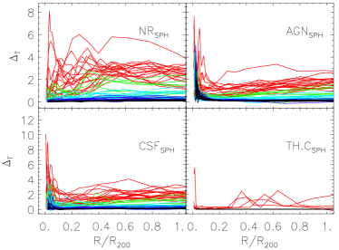
Figure 3: Profiles of temperature variation, $\Delta_{T}=$ $T_{\rm{MW}}$$-$ $T_{\rm{SL}}$, for the different sets of simulated SPH clusters. Line color varies with cluster mass: black lines for $M_{200}<10^{14}$ $h^{-1}M_{\odot}$; blue for $M_{200}$ in the range $[1\div 2]\times 10^{14}$ $h^{-1}M_{\odot}$; cyan for $M_{200}$ in the range $[2\div 5]\times 10^{14}$ $h^{-1}M_{\odot}$; green for $M_{200}$ in the range $[5\div 10]\times 10^{14}$ $h^{-1}M_{\odot}$; and red for $M_{200}>10^{15}$ $h^{-1}M_{\odot}$.

This fraction is reduced in radiative simulations as a consequence of the gas cooling mentioned above. By comparing the simulations with and without AGN feedback, we find that AGNs reduce the temperature variation by 35%.

Thermal conduction, on the other hand, almost completely homogenizes the ICM temperature structure. Even the profiles of the most massive clusters are essentially flat and consistent with no perturbations. The infall of substructures generates only localized peaks but it does not cause long-lasting consequences for the thermal structure of the diffuse medium. $\Delta_{T}$ is always below 0.5 keV at $R_{200}$ with the exception of one object that is experiencing a merging at $z=0$. In addition, temperature inhomogeneities are strongly reduced in the central regions, including the core. This behavior explains the absence of a significant contribution of the temperature bias to the measurement of X-ray mass bias as found by M10.

3.3 Adaptive-mesh Refinement

In the right column of Figure 1, we report the temperature variation as a function of the mass-weighted temperature for the I and O regions of the AMR clusters. Focusing first on the nonradiative results (red line) allows us to evaluate the different predictions of the Eulerian code with respect to the Lagrangian one. The ${\rm NR_{AMR}}$ slopes are always shallower by 40%-100% (Table 2) than the ${\rm NR_{SPH}}$ slopes (Table 1). This could be explained by the larger amount of mixing in the AMR code, which makes the stripping of low-temperature and loosely bound cells more effective. This leads to dissolution of merging substructures and reduction of gaseous inhomogeneties toward the inner region of the clusters. Within $R_{2500}$, indeed, ${\rm NR_{AMR}}$ simulations show the equality between $T_{\rm{MW}}$ and $T_{\rm{SL}}$ ($B\sim 0$ in Table 2), suggesting that the ICM is thermally homogeneous. On the other hand, the SPH simulations show larger temperature variations because merging substructures are more persistent to disruption due to the lack of thermal diffusion (e.g., Frenk et al., 1999; O’Shea et al., 2005; Power et al., 2014, and references therein). As in the particle-based codes, the slope of the $T_{\rm{MW}}$$-\Delta_{T}$ relation increases in moving from the I region to the O (Table 2).

Table 2: AMR Set: Best-fit Parameters, their 1 $\sigma$ Errors, and Scatter of the Linear Relation $\Delta_{T}$=$T_{\rm{MW}}$-$T_{\rm{SL}}$$=A+B\times$($T_{\rm{MW}}$)

all clusters
	A$\pm$ err(A)	B $\pm$ err(B)	scatter
${\rm NR_{AMR}}$, I	-0.06 $\pm$ 0.10	-0.02 $\pm$ 0.02	0.20
${\rm NR_{AMR}}$, M	-0.13 $\pm$ 0.16	0.16 $\pm$ 0.05	0.33
${\rm NR_{AMR}}$, O	-0.44 $\pm$ 0.18	0.47 $\pm$ 0.07	0.38
${\rm CSF_{AMR}}$, I	-2.0 $\pm$ 0.35	0.65 $\pm$ 0.06	0.65
${\rm CSF_{AMR}}$, M	-0.27 $\pm$ 0.11	0.14 $\pm$ 0.03	0.23
${\rm CSF_{AMR}}$, O	-0.19 $\pm$ 0.05	0.18 $\pm$ 0.02	0.12
only relaxed
	A$\pm$ err(A)	B $\pm$ err(B)	scatter
${\rm NR_{AMR}}$, I	-0.05 $\pm$ 0.06	-0.07 $\pm$ 0.02	0.09
${\rm NR_{AMR}}$, M	-0.03 $\pm$ 0.17	0.05 $\pm$ 0.07	0.24
${\rm NR_{AMR}}$, O	-0.01 $\pm$ 0.21	0.09 $\pm$ 0.13	0.29
${\rm CSF_{AMR}}$, I	-1.95 $\pm$ 0.36	0.60 $\pm$ 0.07	0.43
${\rm CSF_{AMR}}$, M	-0.05 $\pm$ 0.04	0.02 $\pm$ 0.01	0.04
${\rm CSF_{AMR}}$, O	-0.03 $\pm$ 0.03	0.05 $\pm$ 0.02	0.04

Relaxed clusters are defined in Section 6.1

Radiative simulations are shown in green in Figure 1. In this case, a direct comparison with the SPH results is less straightforward given the differences in the subgrid model of supernova feedback (kinetic for SPH simulation and thermal for AMR). Nonetheless, there are a few general results we can glean from these comparisons. We find that while SPH and AMR respond similarly in the M and O regions, they do contrast in the innermost part of the clusters. The majority of the discrepancies between the mass-weighted temperature and the spectroscopic-like one is generated in the core of the AMR clusters (Figure 4) whereas in the same region the temperature variations for SPH clusters are generally smaller and limited to the innermost radial bins of hot systems (Figure 3). The $T_{\rm{MW}}$$-\Delta T$ relation for ${\rm CSF_{AMR}}$ has a slope that is significantly steeper than that of the ${\rm CSF_{SPH}}$ simulations (Figure 1). Once the central 10% of $R_{200}$ ($\sim$15% of $R_{500}$) is removed the amplitude $\Delta_{T}$ of AMR simulations drops. Indeed, the majority of the systems show small temperature variations $\Delta_{T}\lesssim 1$ keV of the ICM outside the core (bottom-right panel of Figure 4).

Dividing the set of simulated clusters in mass bins, we find that SPH and AMR codes produce similar temperature variation ($\Delta_{T}\simeq 0.2-0.3$ keV at $R_{500}$ and $R_{200}$) for clusters with $M_{200}<5\times 10^{14}$$h^{-1}M_{\odot}$, whereas the results differ considerably ($\Delta_{T}\simeq$ 0.7–1 keV for AMR and $\Delta_{T}\simeq$2.5 keV for SPH) for more massive objects.

Finally, the AMR mixing being efficient both in nonradiative and radiative simulations, we find that the spectroscopic-like determination of AMR clusters is less influenced by the physics than for SPH simulations (left panel of Figure 4 compared with left panel of Figure 2).

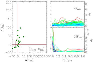
Figure 4: Left panel: difference between the temperatures measured within AMR simulations of N07: the radiative case is compared to nonradiative one, similar to Figure 2. Right panel: profiles of temperature variation, $\Delta_{T}=$ $T_{\rm{MW}}$-$T_{\rm{SL}}$, for the different sets of simulated AMR clusters. Color code as in Figure 3.

4 Characterization of thermal structures

In the previous section, we show that the more efficient mixing of mesh-based codes reduces the temperature variations of AMR clusters. At the same time, by converting the low-entropy gas into stars through the cooling and star formation processes, radiative simulations are characterized by a less thermally perturbed ICM. In this section, we evaluate how temperature inhomogeneities relate to density perturbations.

4.1 Log-normal Distributions

The density, pressure, and temperature distributions of the simulated ICM are approximately log-normal (Rasia et al., 2006; Kawahara et al., 2007; Khedekar et al., 2013; Zhuravleva et al., 2013) with secondary peaks in correspondence of subclumps.

We calculate the (decimal-base) logarithmic gas density and temperature distributions in logarithmically equispaced radial shells. We call $\rho_{G}$ and $T_{G}$ the centers of the respective Gaussian distributions and $\sigma_{\rho}$ and $\sigma_{kT}$ their standard deviations.

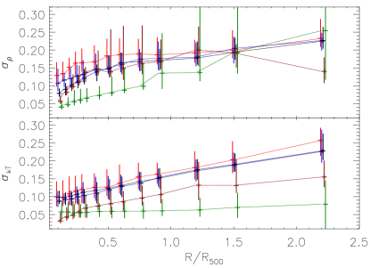
Figure 5: Radial profiles of the median widths of density and temperature log-normal distributions. Vertical bars span from the first to the third quartile. Red, blue, black, brown, and green refer, respectively, to ${\rm NR_{SPH}}$, ${\rm CSF_{SPH}}$, ${\rm AGN_{SPH}}$, ${\rm NR_{AMR}}$, and ${\rm CSF_{AMR}}$.

In Figure 5 we show the median radial profile of the density and temperature dispersions. The temperature dispersion profiles confirm the results outlined in Section 3. The density dispersion profiles are close to one another, especially at a large distance from the center. For $r>0.3\times R_{500}$, the $\sigma_{\rho}$ profile of the ${\rm NR_{AMR}}$simulations is consistent with all profiles of the SPH set. For $r>0.7\times R_{500}$, the ${\rm CSF_{AMR}}$ also agree within the errors. In other words, the degree of substructures, which increases the width of the gas density distribution, is comparable in the two codes. Despite this, SPH clusters are characterized by a higher level of temperature fluctuations. This suggests that the SPH temperature structure, generated by the presence of dense clumps, is further perturbed by other phenomena such as the persistence of the cold stripped gas. This is particularly evident in the innermost region where ${\rm NR_{AMR}}$ and ${\rm NR_{SPH}}$ depart from one another. The reduced density dispersion in the AMR simulations further proves the ability by the mesh-code to disrupt infalling substructures, to quickly thermalize the stripped gas, and to maintain homogenous the cluster central regions.

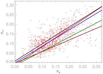
Figure 6: Correspondence between $\sigma_{\rho}$ and $\sigma_{kT}$ measured in each radial shell. For clarity, we plot the points only for ${\rm NR_{AMR}}$ and omit the data points of the other physics whose best-fit linear relations (Equation (2)) are, however, shown with the same color code as in Figure 5.

Another representation of this situation is presented in Figure 6 where we plot the best-fit relations of the density dispersion versus the temperature dispersion:

$${\rm for\ \ NR_{SPH}:}\ \ \sigma_{kT}=0.95\times\sigma_{\rho}-0.01;$$

$${\rm for\ \ CSF_{SPH}:}\ \ \sigma_{kT}=0.85\times\sigma_{\rho};$$

$${\rm for\ \ AGN_{SPH}:}\ \ \sigma_{kT}=0.89\times\sigma_{\rho};$$ (2)

$${\rm for\ \ NR_{AMR}:}\ \ \sigma_{kT}=0.60\times\sigma_{\rho};$$

$${\rm for\ \ CSF_{AMR}:}\ \ \sigma_{kT}=0.74\times\sigma_{\rho}-0.01.$$

The linear fits are derived using a bisector approach. At parity of density fluctuations, SPH clusters have higher temperature fluctuations. For example, for $\sigma_{\rho}\approx 0.2$, the SPH temperature dispersion is 30%–50% above the value of AMR systems.

4.2 Is the Cold Gas in pressure equilibrium?

The connection between density and temperature dispersions is not enough to determine whether the perturbations are isobaric. If we assume that clusters have an onion structure and that the density and temperature of each radial shell is equal to $\rho_{G}$ and $T_{G}$, we find that the two quantities are highly correlated with a positive Pearson correlation coefficient: $\xi_{G}\equiv\xi(\rho_{G},T_{G})=$0.5–0.8. The gas density decreases toward the outskirts as the temperature does. If any fluctuation is completely isobaric, the presence of subclumps will not change the pressure of the ICM. In this situation, the pressure distribution within each shell should have a negligible dispersion.

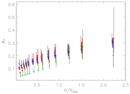
Figure 7: Radial profile of the median widths of the pressure log-normal distributions. Vertical bars span from the first to the third quartile. The color code is that of Figure 5.

In Figure 7, we plot the pressure dispersion obtained from the log-normal fitting of the pressure distributions extracted in the same radial bins as in Figure 5. By comparing the two figures, we notice that the pressure dispersion is even larger than the individual density and temperature dispersions, especially in the external radii. Zhuravleva et al. (2013) explained this behavior by the increasing role with radius of sound waves and weak shocks as indicated by the ratio of the kinetic and thermal energies that changed from more isobaric in the core to more adiabatic farther away.

The above test illustrates that the gas deviating from the average behavior is not in pressure equilibrium. However, the test refers to all perturbations with temperature higher as well as lower than the average. We now focus only on the cold gas because it is it is the responsible for the X-ray temperature bias. For this purpose, we compute the correlation coefficient between the density and the temperature of the 5% coldest gas in each of the regions I, M, and O. The results are shown in Figure 8.

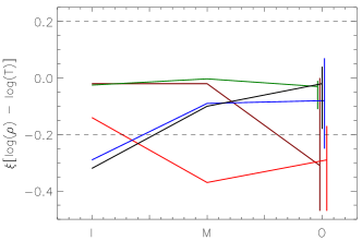
Figure 8: Median of the correlation coefficients between the gas density and temperature of the 5% coldest gas in each of the three regions I, M, and O. Only the median values of the are shown. For the O region, we also overplot the distance between the first and third quartiles as measure of the variance of the sample. The color code is the same of Figure 5.

In the majority of the simulations and regions, the values of $\xi$ are between $-0.20$ and 0.20 indicating no correlation between the temperature and the density of the coldest gas. Isobaric perturbations are possible in the external regions of nonradiative simulations and in the central region of the SPH radiative simulations. In the NR samples, the coldest gas is likely associated with dense merging substructures. The survival time is longer in ${\rm NR_{SPH}}$ simulations, producing $\xi<-0.2$ even in the M region, while the efficient mixing of ${\rm NR_{AMR}}$  reduces the presence of cold clumps already at $R_{500}$. Moving inward. the amount of dispersion in the temperature distribution decreases and the coldest gas is no longer exclusively associated with clumps. The negative $\xi$ in the inner region of SPH radiative clusters is, instead, caused by the presence of a colder and denser core. We repeat the calculation of the correlation coefficient by accounting for the 10% and the 25% of the coldest gas in each region. The qualitative tendency of the results holds. In conclusion, there is no evidence that perturbations, and specifically cold inhomogeneities, are in pressure equilibrium among them or with the diffuse medium.

5 Comparison with Observations

5.1 Characterization of Density and Temperature Distribution.

To compare with the results of Frank et al. (2013) we follow their approach, create the emission-measure-temperature distribution, and compute the median value, $T_{\rm med}$, and the dispersion, $\sigma_{kT,EM}$:

$$\sigma_{kT,EM}=\sqrt{\frac{\sum_{i}[kT_{i}-\langle kT\rangle]\times EM_{i}}{\sum_{i}EM_{i}}}\,,$$ (3)

where $\langle kT\rangle=\Sigma_{i}(kT_{i}\times EM_{i})/\Sigma_{i}(EM_{i})$ is the mean of the emission-measure-weighted temperatures and the emission measure is defined as $EM=m\times\rho$ (see also Biffi et al., 2012).

Figure 9 compares the width of the temperature distribution of ${\rm CSF_{SPH}}$, ${\rm CSF_{AMR}}$, and ${\rm TH.C_{SPH}}$ simulated clusters, calculated according to Equation (3), and the results of XMM–Newton observations by F13. The temperature distribution analysis is carried out in the inner region ($r<R_{2500}$) of clusters. Results related to the nonradiative simulations or to the other regions are reported in Tables 3 and 4 for SPH and AMR, respectively. For reference, we computed the best-fit linear relation following a Bayesian approach (Kelly, 2007) to the sample analyzed by F13 selecting only objects with $T_{\rm med}<7.5$ keV. Simulations conducted by F13, indeed, showed that, in this range, the temperature derived via the smoothed-particle interference technique is trustable at better than 10% while it is biased for hotter objects in part because the lack of sensitivity of XMM–Newton at higher energies (see Figure 9 of F13). The resulting relation is $\sigma_{kT}=0.60^{(\pm 0.2)}+0.27^{(\pm 0.05)}\times kT_{\rm med}$ (black line and shaded gray area in Figure 9).

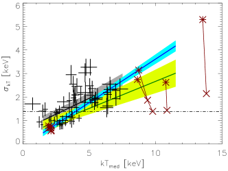
Figure 9: Relation between width of the temperature distribution, $\sigma_{kT}$, and median cluster temperature for the I region. F13 data points, the corresponding best fit ($\sigma_{kT}=0.60{(\pm 0.2)}+0.27{(\pm 0.05)}\times kT_{\rm med}$), and 1$\sigma$ uncertainty are given by the black crosses, black line, and gray region, respectively. The best-fit relations and uncertainties for the inner regions of simulated clusters are shown in blue for ${\rm CSF_{SPH}}$ (Table 4) and green for ${\rm CSF_{AMR}}$(Table 5). Brown asterisks and crosses refer to the nine clusters simulated with and without thermal conduction, respectively.

The comparison with numerical simulations demonstrates that CSF simulations are in reasonable agreement with the results by F13 over the temperature range probed by the current observations ($\simeq$ 2–7 keV). A word of caution, however, needs to be added because the probed region is affected by modeling uncertainties. Indeed, the origin of the temperature inhomogeneities in the I region is different in AMR and in SPH: while for AMR it is mostly due to the large temperature variation present in the cluster core (Figure 4), for SPH simulations it is caused by the survival of substructures and their stripped gas (Figure 3). The remarkable influence of the core on AMR simulations is clear by comparing Figures 9 and 10. The latter refers to the same I region with the core (defined as $R<0.15\times R_{500}$) removed.

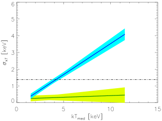
Figure 10: Best-fit relations and uncertainties of the I regions of ${\rm CSF_{SPH}}$  clusters (blue) and ${\rm CSF_{AMR}}$ objects (green) once the central $0.15\times R_{500}$ are excised.

Including AGN feedback in SPH simulations slightly reduces the width of the temperature distribution, because AGNs expel gas from the substructures decreasing the ICM temperature inhomogeneity. The resulting $\sigma_{kT}-T$ relation becomes very similar to the observed one (see Table 3).

Thermal conduction reduces the values of $\sigma_{kT}$, especially at high temperature, where conductivity becomes efficient (Dolag et al., 2004). The corresponding $\sigma_{kT}$–$T$ relation is shallower than the extrapolation of the observed one, suggesting that measurements of the ICM temperature distribution of very hot clusters (currently not available) can be used to constrain the degree of thermal conduction in the intracluster plasma.

Table 3: SPH set: best-fit parameters, their 1 $\sigma$ errors, and scatter of the linear relation: $\sigma_{kT}=A+B\times kT_{\rm med}$

all clusters
	A$\pm$ err(A)	B $\pm$ err(B)	scatter
${\rm NR_{SPH}}$, I	-0.32$\pm$ 0.19	0.43 $\pm$ 0.03	0.58
${\rm NR_{SPH}}$, M	-0.36$\pm$ 0.13	0.63 $\pm$ 0.03	0.38
${\rm NR_{SPH}}$, O	-0.20 $\pm$ 0.14	0.64 $\pm$ 0.04	0.40
${\rm CSF_{SPH}}$, I	-0.15$\pm$ 0.24	0.38 $\pm$ 0.04	0.67
${\rm CSF_{SPH}}$, M	-0.46$\pm$ 0.18	0.55 $\pm$ 0.04	0.51
${\rm CSF_{SPH}}$, O	-0.37 $\pm$ 0.12	0.68 $\pm$ 0.03	0.35
${\rm AGN_{SPH}}$, I	0.05 $\pm$ 0.17	0.34 $\pm$ 0.03	0.47
${\rm AGN_{SPH}}$,M	-0.37 $\pm$ 0.16	0.51 $\pm$ 0.03	0.46
${\rm AGN_{SPH}}$, O	-0.41 $\pm$ 0.11	0.70 $\pm$ 0.03	0.31
${\rm TH.C_{SPH}}$, I	0.26 $\pm$ 0.09	0.13 $\pm$ 0.01	0.05
${\rm TH.C_{SPH}}$, M	-0.13 $\pm$ 0.07	0.29 $\pm$ 0.01	0.04
${\rm TH.C_{SPH}}$, O	-0.06 $\pm$ 0.02	0.27 $\pm$ 0.01	0.02
only relaxed
	A$\pm$ err(A)	B $\pm$ err(B)	scatter
${\rm NR_{SPH}}$, I	-0.45$\pm$ 0.20	0.34 $\pm$ 0.04	0.29
${\rm NR_{SPH}}$, M	-0.60$\pm$ 0.20	0.63 $\pm$ 0.04	0.28
${\rm NR_{SPH}}$, O	-0.29 $\pm$ 0.09	0.66 $\pm$ 0.03	0.12
${\rm CSF_{SPH}}$, I	0.24$\pm$ 0.25	0.21 $\pm$ 0.04	0.33
${\rm CSF_{SPH}}$, M	-0.30$\pm$ 0.21	0.41 $\pm$ 0.04	0.29
${\rm CSF_{SPH}}$, O	-0.71 $\pm$ 0.09	0.75 $\pm$ 0.03	0.12
${\rm AGN_{SPH}}$, I	0.41 $\pm$ 0.15	0.22 $\pm$ 0.02	0.20
${\rm AGN_{SPH}}$,M	-0.34 $\pm$ 0.14	0.40 $\pm$ 0.03	0.19
${\rm AGN_{SPH}}$, O	-0.57 $\pm$ 0.10	0.69 $\pm$ 0.03	0.12

Relaxed clusters are defined in Section 6.1

Table 4: AMR set: best-fit parameters, their 1 $\sigma$ errors, and scatter of the linear relation: $\sigma_{kT}=A+B\times kT_{\rm med}$

all clusters
	A$\pm$ err(A)	B $\pm$ err(B)	scatter
${\rm NR_{AMR}}$, I	0.04$\pm$ 0.10	0.23 $\pm$ 0.02	0.22
${\rm NR_{AMR}}$, M	-0.19$\pm$ 0.12	0.38 $\pm$ 0.04	0.24
${\rm NR_{AMR}}$, O	-0.12 $\pm$ 0.12	0.50 $\pm$ 0.05	0.26
${\rm CSF_{AMR}}$, I	0.37 $\pm$ 0.27	0.23 $\pm$ 0.05	0.51
${\rm CSF_{AMR}}$, M	-0.17 $\pm$ 0.09	0.32 $\pm$ 0.02	0.18
${\rm CSF_{AMR}}$, O	-0.40 $\pm$ 0.18	0.59$\pm$ 0.07	0.40
only relaxed
	A$\pm$ err(A)	B $\pm$ err(B)	scatter
${\rm NR_{AMR}}$, I	0.21$\pm$ 0.07	0.17 $\pm$ 0.02	0.10
${\rm NR_{AMR}}$, M	-0.03$\pm$ 0.14	0.24 $\pm$ 0.06	0.20
${\rm NR_{AMR}}$, O	0.15 $\pm$ 0.13	0.25 $\pm$ 0.08	0.18
${\rm CSF_{AMR}}$, I	0.61 $\pm$ 0.32	0.17 $\pm$ 0.06	0.38
${\rm CSF_{AMR}}$, M	0.01 $\pm$ 0.10	0.22 $\pm$ 0.03	0.11
${\rm CSF_{AMR}}$, O	0.08 $\pm$ 0.09	0.22$\pm$ 0.05	0.11

Relaxed clusters are defined in Section 6.1

6 Consequences for the X-ray mass

Using the gas as a tracer and assuming HE, the total mass of a system within a certain radius $r$ is calculated as

$$M(<r)=-\frac{rT(r)}{\mu m_{p}G}\times\left[\frac{d\log\rho_{gas}}{d\log r}+\frac{d\log T}{d\log r}\right],$$ (4)

where the temperature and the derivatives are computed at the radius $r$, $\mu\approx 0.59$ is the mean molecular weight, $m_{p}$ is the proton mass, and $G$ is the gravitational constant. Several works based on simulations already pointed out that on top of the thermal pressure another term is needed to counterbalance the gravity accounting for 10%–15% of the total mass (see Ettori et al., 2013, for a review on X-ray mass measurement). In this section, using the simulations with radiative physics, we estimate the potential extra contribution generated by the X-ray temperature bias (Rasia et al., 2006, R12). For this purpose, we derive the mass by adopting both the mass-weighted temperature and the spectroscopic-like one. We call $M_{MW}$ and $M_{SL}$ the respective masses at $R_{500}$.

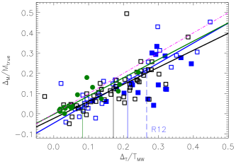
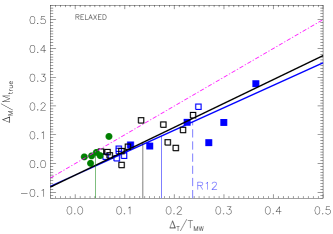
Figure 11: Mass bias, $(\Delta_{M}=M_{MW}-M_{SL})/M_{\rm true}$, versus temperature bias, $(\Delta_{T}=T_{MW}-T_{SL})/T_{MW}$ at $R_{500}$. The entire samples are shown in the left panel, and only relaxed objects are isolated in the right panel. Green circles and lines refer to ${\rm CSF_{AMR}}$. Blue and black squares and lines show ${\rm CSF_{SPH}}$ and ${\rm AGN_{SPH}}$, respectively. The magenta line represents the identity relation. The median values of the temperature bias are plotted as vertical lines. The rightmost dashed blue line corresponds to the R12 sample identified by the filled blue squares. The bisector best fit relations in the form $\Delta_{M}/M_{\rm true}=A+B\times\Delta_{T}/T_{MW}$ have parameters $(A;B)=(0;0.9)$ for ${\rm CSF_{AMR}}$; $(A;B)=(-0.07;1.07)$ for ${\rm CSF_{SPH}}$ and $(A;B)=(-0.04;0.91)$ for ${\rm AGN_{SPH}}$. The AGN relation changes only slightly for relaxed objects while the slope of ${\rm CSF_{SPH}}$decreases to 0.8.

The relation between the temperature variation normalized to the mass-weighted temperature and the normalized mass variation is shown in Figure 11. Once again, while minor differences are detected between the two SPH feedback mechanisms (${\rm CSF_{SPH}}$ versus ${\rm AGN_{SPH}}$), we notice a separation between the normalization of SPH and AMR simulations: at fixed $\Delta_{T}$$T_{\rm{MW}}$ AMR clusters have a larger $\Delta_{M}/M_{\rm true}$ associated with them. The explanation relies on the fact that around $R_{500}$, the $T_{SL}$ profile is steeper than the $T_{MW}$ profile for SPH simulated clusters. The temperature derivative, within the $M_{SL}$ expression, is, thus, more negative and as such the mass bias is effectively reduced. With vertical lines, we report the median values of the relative temperature variations of the radiative samples. The mass bias of the R12 sample is, on average, the most affected by temperature inhomogeneities because the sample contains massive systems that are experiencing several merging events. The set of M10 is not shown in the figure, however, the effect of thermal conduction is such to locate all nine clusters in the same position in the plane: $\Delta_{T}/$$T_{\rm{MW}}$ $\sim\Delta_{M}/M_{\rm true}<0.12$.

As a final step, we study how the points move in the mass $-$ temperature plane according to the two temperature definitions. We derive the linear fit in the form $\log(M)=N+\alpha\times\log(T)$ for the following relations: $M_{\rm true}-T_{\rm MW}$, $M_{\rm MW}-T_{\rm MW}$, and $M_{\rm SL}-T_{\rm SL}$. The power-law index $\alpha\approx 1.5-1.6$ is always consistent within 1 $\sigma$ error among the three relations for all radiative simulations. The normalizations, $10^{N}$, of the second and third relations vary with respect to the first case according to the median ratios $M_{\rm MW}/M_{\rm true}$ and $M_{\rm SL}/M_{\rm true}$. Respectively, these are equal to 15% and 20% in SPH and they are about 5% in AMR.

6.1 Relaxed sample

In this section, we restrict the study of the mass bias to relaxed systems. Simulations show that the degree of inhomogeneities in the medium depends on the dynamical state of the cluster. For example, recently, Vazza et al. (2013) showed that the baryon fraction can be twice as biased in perturbed systems. At the same time, Zhuravleva et al. (2013) demonstrated that the gas density distribution of unrelaxed clusters is higher with respect to relaxed clusters in a large interval of radii ([$R_{2500}\div R_{200}$]) and that the peaks of the distributions of relaxed and perturbed systems have a significant separation.

In the radiative sample, we define the relaxation of a cluster on the basis of the X-ray morphology. For the ${\rm CSF_{AMR}}$ set, we adopt the classification of Khedekar et al. (2013) and Zhuravleva et al. (2013) where 6 objects out of 16 are visually recognized as X-ray regular. For the SPH samples, we measure the global X-ray morphological parameter, $M_{\rm par}$ (Rasia et al., 2013; Meneghetti et al., 2014), and impose $M_{\rm par}<-1$. In the Appendix, this selection method is compared with the mass-accretion-history parameter $\Gamma$ (e.g. Diemer et al., 2013). The relaxed samples of SPH are composed by the 12 objects that satisfy the condition in all of the three physics.

The relations analyzed in Sections 3 and 5 are rederived considering regular systems (see bottom part of all tables). The results for SPH simulations change slightly, often favoring a smaller normalization. In most of the cases, the relations of the entire sample and those of relaxed objects are consistent within 1$\sigma$ whenever the $T_{\rm{MW}}$ of the clusters is $T_{\rm MW}\leq 5$ keV whereas massive perturbed objects have higher temperature variation $\Delta_{T}$ and temperature dispersion $\sigma_{kT}$. The $T_{\rm{MW}}$$-\Delta_{T}$ normalization and slope of the AMR relaxed systems change more drastically being always consistent with zero (with the exception of the central region). For each physics and region, the $T_{\rm{MW}}$$-\sigma_{kT}$ relation is also shallower. At fixed $T_{\rm{MW}}$ the value of $\sigma_{kT}$ is lower by 10% for $T_{\rm{MW}}$$\leq 2$ keV, $20\%-25\%$ for $T_{\rm{MW}}$$=3-4$ keV, and $25\%-30\%$ for $T_{\rm{MW}}$$\geq 5$ keV.

In the right panel of Figure 11 we plot the influence of the temperature variation on the mass bias for relaxed samples. As expected, the ${\rm CSF_{AMR}}$ systems are distinguished by a low degree of both temperature and mass variation. In this case, for the reduced range of both axes, we are not able to linearly fit the points. For ${\rm CSF_{SPH}}$ simulations, the slope of the $\Delta_{M}/M_{\rm true}-\Delta_{T}/$$T_{\rm{MW}}$ relation decreases by 20% with respect to the entire sample. The mean temperature variation of relaxed objects corresponds to a mass bias that is about half the mass bias of the total sample.

7 Conclusions

Motivated by the discrepant results by N07, M10, and R12 on the HE mass bias, we evaluate the degrees of temperature inhomogeneities present in their simulated sets. Structures in the ICM temperature distribution are, indeed, the main sources of systematic bias in the X-ray spectroscopic temperature measurement with direct consequences for the HE mass estimate of X–ray clusters. We analyzed four different samples simulated with either GADGET, an SPH code, or ART, an AMR algorithm. The simulations implement various prescriptions for the baryonic physics, including nonradiative gas and processes of cooling, star formation and feedback by supernovae or AGNs. A small sample of nine objects allowed us to study the effect of thermal conduction. After comparing the degree of temperature structure and studying its nature, we tested the predictions against the observational results of Frank et al. (2013) and derived our conclusions on the consequences of the X-ray mass bias. Our main results can be summarized as follows:

• AMR simulations with nonradiative physics predict a lower degree of ICM temperature inhomogeneities with respect to SPH because the more efficient mixing destroys substructures during their infall within the cluster and quickly thermalizes the stripped gas.

• The effect of baryonic physics in radiative simulations substantially reduces the differences between AMR and SPH simulations. Radiative cooling removes cold and dense gas from its diffuse state, thus reducing the entropy contrast of the ICM. However, the discrepancies between the simulated sets are still significant at small radii ($R<R_{2500}$) mostly because of the complex physics of the core and the different implementations of the stellar feedback. ${\rm CSF_{SPH}}$  and ${\rm AGN_{SPH}}$  simulations show similar response to temperature variations even if there is a systematic tendency to have less inhomogeneity in the presence of AGN. The inclusion of kinetic feedback in the AGN model might, however, increase this difference. Thermal conduction drastically smooths temperature variations and homogenizes the ICM.

• AMR and SPH produce a comparable amount of density inhomogeneities, especially in the nonradiative case and in the external regions (outside $\sim 0.7\times R_{500}$). However, a fixed amount of density inhomogeneities presents a higher degree of temperature perturbations in SPH clusters.

• The cold gas of nonradiative simulations is associated with dense clumps mostly connected to merging substructures. The radiative simulations instead present a negligible correlation between the temperature and density. This confirms the idea that the coldest gas is not in pressure equilibrium with the diffuse gas.

• The emission-measure temperature dispersions of radiative simulations carried out by both codes match equally well the observational data of F13 even if for different reasons: the dispersion of AMR clusters depends on the core physics while that of SPH is caused by the survival of substructures and the cold stripped gas.
  From an observational point of view, more insights on the ICM processes might be provided by masking the core of observed clusters. In this case, AMR clusters show a temperature dispersion consistent with zero over the entire temperature range while the $kT_{med}-\sigma_{kt}$ relation of SPH systems does not change significantly. Another solution could be to measure temperature variation at distances larger than $R_{2500}$. Indeed, the predicted dispersion grows rapidly with the radius: in the M region the difference in $\sigma_{kT}$ between AMR and SPH increases by at least $\sim$ 60% for all systems with temperature $T[R_{2500}-R_{500}]>2$ keV. Finally, the difference between AMR and SPH becomes more evident for high–temperature clusters. For example, the difference between the predicted AMR and SPH dispersions is 16% for a 5 keV cluster and grows up to 30% for an 8 keV one.

• The consequences for the X-ray mass bias caused by thermal fluctuations are similar among the radiative simulations. However, because the temperature variations are smaller in AMR simulations, their mass bias can be a factor of two lower. The difference is even more marked when the sample of N07 is compared to R12 because the latter has massive objects with heavily disturbed ICM.

• As expected, relaxed objects present lower degrees of inhomogeneities, especially for AMR simulations.

The exact determination of the temperature bias is sought because its contribution to the X–ray mass bias might be as high as non-thermal pressure support associated with ICM bulk motions (R12, Planck Collaboration 2013). Upcoming high–resolution X–ray spectroscopic observations, e.g., with ASTRO-H, will help characterize gas motions with direct implications for the mass calibration of clusters. At the same time, detailed X–ray observations would be necessary to extend the current description of ICM thermal fluctuation to larger radii and including hotter systems. While pushing the capabilities of the current generation of instruments to their limits will be beneficial, a leap forward in these studies will be reached with the advent of a next generation of high–sensitivity X–ray telescopes such as the Athena+ X-ray observatory (Nandra et al., 2013; Pointecouteau et al., 2013).

Appendix A Selection of relaxed cluster.

Using the ${\rm NR_{SPH}}$, ${\rm CSF_{SPH}}$, and ${\rm AGN_{SPH}}$ sets, we compare two approaches to select relaxed systems: the first, more theoretical, uses the mass-accretion parameter, $\Gamma$ (e.g. Vazza et al., 2013; Diemer & Kravtsov, 2014), and the second, observationally oriented, considers the global morphological parameter, $M_{par}$(Rasia et al., 2013).

Dynamical state. The mass-accretion-rate parameter is a measure of the mass increase of an object with time:

$$\Gamma=\frac{\log M_{500}(z_{2})-\log M_{500}(z_{1})}{\log(1+z_{1})-\log(1+z_{2})}$$ (A1)

where the mass at redshift $z_{2}$ refers to the most massive progenitor of the cluster at redshift $z_{1}<z_{2}$. The redshift of reference, $z_{1}$, corresponds to the one used in this work and it is set equal to zero while $z_{2}$ is fixed to 0.25. The redshift difference corresponds to 3 Gyr: a sufficient time to allow a substructure that merged before or around $z_{2}$ to be completely incorporated into the main cluster but not enough time to allow a substructure that merged afterwards to relax (Nelson et al., 2014). The values of the $\Gamma$ parameters are not influenced by the ICM physics. We consider $\Gamma=2$ as the threshold to distinguish between relaxed and perturbed objects. This factor corresponds to a mass increase of about 35% between redshift $z_{2}$ and $z_{1}$, equal to the factor attributable only to the pseudo-evolution of clusters (Diemer et al., 2013).

X-ray regularity: morphological parameters. The X-ray regularity is estimated through the global morphological parameter, $M_{par}$, defined as

$$M_{par}=\sum{\frac{X-<X>}{\sigma_{X}}}$$ (A2)

where $X$ represents an ensemble of morphological parameters, ¡¿ denotes the mean values of the distribution of each parameter, and $\sigma$ their standard deviation. The morphological estimators used are: the centroid shift, $w$ (Mohr et al., 1993); the ellipticity, $\epsilon$; the X-ray surface brightness concentration (Cassano et al., 2010); and the third and fourth power ratios, $P_{3}$ and $P_{4}$ (Buote & Tsai, 1995), such that $X\equiv[\log w,\log 1/c,\log P_{3},\log P_{4},\epsilon]$. The means and standard deviations of our ${\rm NR_{SPH}}$ samples are comparable with those derived by Meneghetti et al. (2014) who analyzed a much larger sample taken from the MUSIC simulations (Sembolini et al., 2013). Objects with $M_{par}$ below zero are by definition more regular than the average. To be more restrictive we impose the limit of $M_{par}<-1$.

Figure 12: Relation between mass-accretion-history parameter, $\Gamma$, and the morphological parameter, $M_{\rm par}$. Horizontal and vertical lines show the limits used to distinguish between dynamically relaxed and unrelaxed objects ($\Gamma=2$) and between X-ray regular and disturbed X-ray images ($M_{\rm par}=-1$).

Interestingly, $\Gamma$ shows a good degree of correlation with the X-ray morphological parameter $M_{\rm par}$: $\xi=0.45-0.5$. In Figure 12 we show the ${\rm AGN_{SPH}}$ case. The points of the other two simulated sets are similarly located. For our samples, objects with $M_{par}<-1$ tend to be dynamically relaxed ($\Gamma<2$) with only few exceptions ($\leq 2$ objects). On the other hand, selecting objects with lower values of $\Gamma$ does not guarantee the X-ray regularity, on the contrary some clusters with $\Gamma<2$ have $M_{\rm par}>3$.

Other criteria to evaluate the dynamical state have been introduced in the literature such as the center of mass displacement (defined as the offset between the center of mass and the minimum of the potential); the virial ratio between the thermal energy plus the surface pressure term and the kinetic energy; and the substructure mass fraction within the virial radius (Neto et al., 2007; Power et al., 2012; Meneghetti et al., 2014). We checked the performance of $M_{par}$ against the offset parameter derived by Killedar et al. (2012) for our SPH set. We verified that also in this case $M_{par}$ is a stronger constraint. We reserve for future investigation a detailed comparison between several dynamical state parameters and the morphological parameters.

The relaxed sample of SPH simulations include 12 clusters that have $M_{par}<-1$ in all of the three physics. This subsample covers a wide range in mass with $M_{200}$ spanning from $8\times 10^{13}$$h^{-1}$$M_{\odot}$ to $1.5\times 10^{13}$$h^{-1}$$M_{\odot}$ and it presents the same number of objects below and above the mass $M_{200}=4\times 10^{14}$$h^{-1}$$M_{\odot}$.

References

- Ameglio et al. (2009) Ameglio, S., Borgani, S., Pierpaoli, E., Dolag, K., Ettori, S., & Morandi, A. 2009, MNRAS, 394, 479
- Balsara (1995) Balsara, D. S. 1995, Journal of Computational Physics, 121, 357
- Bautz et al. (2009) Bautz, M. W., Miller, E. D., Sanders, J. S., Arnaud, K. A., Mushotzky, R. F., Porter, F. S., Hayashida, K., Henry, J. P., Hughes, J. P., Kawaharada, M., Makashima, K., Sato, M., & Tamura, T. 2009, PASJ, 61, 1117
- Becker & Kravtsov (2011) Becker, M. R. & Kravtsov, A. V. 2011, ApJ, 740, 25
- Biffi et al. (2012) Biffi, V., Dolag, K., Böhringer, H., & Lemson, G. 2012, MNRAS, 420, 3545
- Biffi et al. (2014) Biffi, V., Sembolini, F., De Petris, M., Valdarnini, R., Yepes, G., & Gottlöber, S. 2014, MNRAS, 439, 588
- Bonafede et al. (2011) Bonafede, A., Dolag, K., Stasyszyn, F., Murante, G., & Borgani, S. 2011, MNRAS, 418, 2234
- Borgani & Kravtsov (2011) Borgani, S. & Kravtsov, A. 2011, Advanced Science Letters, 4, 204
- Bourdin et al. (2011) Bourdin, H., Arnaud, M., Mazzotta, P., Pratt, G. W., Sauvageot, J.-L., Martino, R., Maurogordato, S., Cappi, A., Ferrari, C., & Benoist, C. 2011, A&A, 527, A21
- Bourdin & Mazzotta (2008) Bourdin, H. & Mazzotta, P. 2008, A&A, 479, 307
- Bourdin et al. (2013) Bourdin, H., Mazzotta, P., Markevitch, M., Giacintucci, S., & Brunetti, G. 2013, ApJ, 764, 82
- Buote & Tsai (1995) Buote, D. A. & Tsai, J. C. 1995, ApJ, 452, 522
- Cassano et al. (2010) Cassano, R., Ettori, S., Giacintucci, S., Brunetti, G., Markevitch, M., Venturi, T., & Gitti, M. 2010, ApJL, 721, L82
- Chabrier (2003) Chabrier, G. 2003, PASP, 115, 763
- Churazov et al. (2012) Churazov, E., Vikhlinin, A., Zhuravleva, I., Schekochihin, A., Parrish, I., Sunyaev, R., Forman, W., Böhringer, H., & Randall, S. 2012, MNRAS, 421, 1123
- Diemer & Kravtsov (2014) Diemer, B. & Kravtsov, A. V. 2014, ApJ, 789, 1
- Diemer et al. (2013) Diemer, B., More, S., & Kravtsov, A. V. 2013, ApJ, 766, 25
- Dolag et al. (2004) Dolag, K., Bartelmann, M., Perrotta, F., Baccigalupi, C., Moscardini, L., Meneghetti, M., & Tormen, G. 2004, A&A, 416, 853
- Dolag et al. (2009) Dolag, K., Borgani, S., Murante, G., & Springel, V. 2009, MNRAS, 399, 497
- Ettori et al. (2013) Ettori, S., Donnarumma, A., Pointecouteau, E., Reiprich, T. H., Giodini, S., Lovisari, L., & Schmidt, R. W. 2013, Space Sci. Rev., 177, 119
- Fabjan et al. (2011) Fabjan, D., Borgani, S., Rasia, E., Bonafede, A., Dolag, K., Murante, G., & Tornatore, L. 2011, MNRAS, 416, 801
- Ferland et al. (1998) Ferland, G. J., Korista, K. T., Verner, D. A., Ferguson, J. W., Kingdon, J. B., & Verner, E. M. 1998, PASP, 110, 761
- Foëx et al. (2012) Foëx, G., Soucail, G., Pointecouteau, E., Arnaud, M., Limousin, M., & Pratt, G. W. 2012, A&A, 546, A106
- Frank et al. (2013) Frank, K. A., Peterson, J. R., Andersson, K., Fabian, A. C., & Sanders, J. S. 2013, ApJ, 764, 46
- Frenk et al. (1999) Frenk, C. S., White, S. D. M., Bode, P., & et al. 1999, ApJ, 525, 554
- Gu et al. (2009) Gu, L., Xu, H., Gu, J., Wang, Y., Zhang, Z., Wang, J., Qin, Z., Cui, H., & Wu, X.-P. 2009, ApJ, 700, 1161
- Haardt & Madau (2001) Haardt, F. & Madau, P. 2001, in Clusters of Galaxies and the High Redshift Universe Observed in X-rays, ed. D. M. Neumann & J. T. V. Tran
- Israel et al. (2014) Israel, H., Reiprich, T. H., Erben, T., Massey, R. J., Sarazin, C. L., Schneider, P., & Vikhlinin, A. 2014, A&A, 564, A129
- Jee et al. (2011) Jee, M. J., Dawson, K. S., Hoekstra, H., Perlmutter, S., Rosati, P., Brodwin, M., Suzuki, N., Koester, B., Postman, M., Lubin, L., Meyers, J., Stanford, S. A., Barbary, K., Barrientos, F., Eisenhardt, P., Ford, H. C., Gilbank, D. G., Gladders, M. D., Gonzalez, A., Harris, D. W., Huang, X., Lidman, C., Rykoff, E. S., Rubin, D., & Spadafora, A. L. 2011, ApJ, 737, 59
- Jeltema et al. (2008) Jeltema, T. E., Hallman, E. J., Burns, J. O., & Motl, P. M. 2008, ApJ, 681, 167
- Jubelgas et al. (2004) Jubelgas, M., Springel, V., & Dolag, K. 2004, MNRAS, 351, 423
- Kawahara et al. (2007) Kawahara, H., Suto, Y., Kitayama, T., Sasaki, S., Shimizu, M., Rasia, E., & Dolag, K. 2007, ApJ, 659, 257
- Kelly (2007) Kelly, B. C. 2007, ApJ, 665, 1489
- Khedekar et al. (2013) Khedekar, S., Churazov, E., Kravtsov, A., Zhuravleva, I., Lau, E. T., Nagai, D., & Sunyaev, R. 2013, MNRAS, 431, 954
- Killedar et al. (2012) Killedar, M., Borgani, S., Meneghetti, M., Dolag, K., Fabjan, D., & Tornatore, L. 2012, MNRAS, 427, 533
- Klypin et al. (2001) Klypin, A., Kravtsov, A. V., Bullock, J. S., & Primack, J. R. 2001, ApJ, 554, 903
- Kravtsov et al. (1997) Kravtsov, A. V., Klypin, A. A., & Khokhlov, A. M. 1997, ApJS, 111, 73
- Lau et al. (2009) Lau, E. T., Kravtsov, A. V., & Nagai, D. 2009, ApJ, 705, 1129
- Mahdavi et al. (2013) Mahdavi, A., Hoekstra, H., Babul, A., Bildfell, C., Jeltema, T., & Henry, J. P. 2013, ApJ, 767, 116
- Mahdavi et al. (2008) Mahdavi, A., Hoekstra, H., Babul, A., & Henry, J. P. 2008, MNRAS, 384, 1567
- Mathiesen & Evrard (2001) Mathiesen, B. F. & Evrard, A. E. 2001, ApJ, 546, 100
- Mazzotta et al. (2004) Mazzotta, P., Rasia, E., Moscardini, L., & Tormen, G. 2004, MNRAS, 354, 10
- Meneghetti et al. (2010) Meneghetti, M., Rasia, E., Merten, J., Bellagamba, F., Ettori, S., Mazzotta, P., Dolag, K., & Marri, S. 2010, A&A, 514, A93
- Meneghetti et al. (2014) Meneghetti, M., Rasia, E., Vega, J., Merten, J., Postman, M., Yepes, G., Sembolini, F., Donahue, M., Ettori, S., Umetsu, K., Balestra, I., Bartelmann, M., Benitez, N., Biviano, A., Bouwens, R., Bradley, L., Broadhurst, T., Coe, D., Czakon, N., De Petris, M., Ford, H., Giocoli, C., Gottloeber, S., Grillo, C., Infante, L., Jouvel, S., Kelson, D., Koekemoer, A., Lahav, O., Lemze, D., Medezinski, E., Melchior, P., Mercurio, A., Molino, A., Moscardini, L., Monna, A., Moustakas, J., Moustakas, L. A., Nonino, M., Rhodes, J., Rosati, P., Sayers, J., Seitz, S., Zheng, W., & Zitrin, A. 2014, ArXiv e-prints
- Mohr et al. (1993) Mohr, J. J., Fabricant, D. G., & Geller, M. J. 1993, ApJ, 413, 492
- Nagai et al. (2007a) Nagai, D., Kravtsov, A. V., & Vikhlinin, A. 2007a, ApJ, 668, 1
- Nagai & Lau (2011) Nagai, D. & Lau, E. T. 2011, ApJL, 731, L10
- Nagai et al. (2007b) Nagai, D., Vikhlinin, A., & Kravtsov, A. V. 2007b, ApJ, 655, 98
- Nandra et al. (2013) Nandra, K., Barret, D., Barcons, X., Fabian, A., den Herder, J.-W., Piro, L., Watson, M., Adami, C., Aird, J., Afonso, J. M., & et al. 2013, ArXiv e-prints
- Nelson et al. (2014) Nelson, K., Lau, E. T., Nagai, D., Rudd, D. H., & Yu, L. 2014, ApJ, 782, 107
- Nelson et al. (2012) Nelson, K., Rudd, D. H., Shaw, L., & Nagai, D. 2012, ApJ, 751, 121
- Neto et al. (2007) Neto, A. F., Gao, L., Bett, P., Cole, S., Navarro, J. F., Frenk, C. S., White, S. D. M., Springel, V., & Jenkins, A. 2007, MNRAS, 381, 1450
- O’Shea et al. (2005) O’Shea, B. W., Nagamine, K., Springel, V., Hernquist, L., & Norman, M. L. 2005, ApJS, 160, 1
- Padovani & Matteucci (1993) Padovani, P. & Matteucci, F. 1993, ApJ, 416, 26
- Peterson et al. (2007) Peterson, J. R., Marshall, P. J., & Andersson, K. 2007, ApJ, 655, 109
- Piffaretti & Valdarnini (2008) Piffaretti, R. & Valdarnini, R. 2008, A&A, 491, 71
- Planck Collaboration et al. (2013) Planck Collaboration, Ade, P. A. R., Aghanim, N., Armitage-Caplan, C., Arnaud, M., Ashdown, M., Atrio-Barandela, F., Aumont, J., Baccigalupi, C., Banday, A. J., & et al. 2013, ArXiv e-prints
- Planelles et al. (2013) Planelles, S., Borgani, S., Dolag, K., Ettori, S., Fabjan, D., Murante, G., & Tornatore, L. 2013, MNRAS, 431, 1487
- Pointecouteau et al. (2013) Pointecouteau, E., Reiprich, T. H., Adami, C., Arnaud, M., Biffi, V., Borgani, S., Borm, K., Bourdin, H., Brueggen, M., Bulbul, E., Clerc, N., Croston, J. H., Dolag, K., Ettori, S., Finoguenov, A., Kaastra, J., Lovisari, L., Maughan, B., Mazzotta, P., Pacaud, F., de Plaa, J., Pratt, G. W., Ramos-Ceja, M., Rasia, E., Sanders, J., Zhang, Y.-Y., Allen, S., Boehringer, H., Brunetti, G., Elbaz, D., Fassbender, R., Hoekstra, H., Hildebrandt, H., Lamer, G., Marrone, D., Mohr, J., Molendi, S., Nevalainen, J., Ohashi, T., Ota, N., Pierre, M., Romer, K., Schindler, S., Schrabback, T., Schwope, A., Smith, R., Springel, V., & von der Linden, A. 2013, ArXiv e-prints
- Power et al. (2012) Power, C., Knebe, A., & Knollmann, S. R. 2012, MNRAS, 419, 1576
- Power et al. (2014) Power, C., Read, J. I., & Hobbs, A. 2014, MNRAS, 440, 3243
- Ragone-Figueroa et al. (2013) Ragone-Figueroa, C., Granato, G. L., Murante, G., Borgani, S., & Cui, W. 2013, MNRAS, 436, 1750
- Rasia et al. (2006) Rasia, E., Ettori, S., Moscardini, L., Mazzotta, P., Borgani, S., Dolag, K., Tormen, G., Cheng, L. M., & Diaferio, A. 2006, MNRAS, 369, 2013
- Rasia et al. (2013) Rasia, E., Meneghetti, M., & Ettori, S. 2013, The Astronomical Review, 8, 40
- Rasia et al. (2012) Rasia, E., Meneghetti, M., Martino, R., Borgani, S., Bonafede, A., Dolag, K., Ettori, S., Fabjan, D., Giocoli, C., Mazzotta, P., Merten, J., Radovich, M., & Tornatore, L. 2012, New Journal of Physics, 14, 055018
- Rasia et al. (2004) Rasia, E., Tormen, G., & Moscardini, L. 2004, MNRAS, 351, 237
- Reiprich et al. (2013) Reiprich, T. H., Basu, K., Ettori, S., Israel, H., Lovisari, L., Molendi, S., Pointecouteau, E., & Roncarelli, M. 2013, Space Sci. Rev., 177, 195
- Reiprich & Böhringer (2002) Reiprich, T. H. & Böhringer, H. 2002, ApJ, 567, 716
- Roncarelli et al. (2013) Roncarelli, M., Ettori, S., Borgani, S., Dolag, K., Fabjan, D., & Moscardini, L. 2013, MNRAS
- Roncarelli et al. (2006) Roncarelli, M., Ettori, S., Dolag, K., Moscardini, L., Borgani, S., & Murante, G. 2006, MNRAS, 373, 1339
- Rossetti et al. (2013) Rossetti, M., Eckert, D., De Grandi, S., Gastaldello, F., Ghizzardi, S., Roediger, E., & Molendi, S. 2013, ArXiv e-prints
- Rudd et al. (2008) Rudd, D. H., Zentner, A. R., & Kravtsov, A. V. 2008, ApJ, 672, 19
- Schenck et al. (2014) Schenck, D., Datta, A., Burns, J., & Skillman, S. 2014, ArXiv e-prints
- Sembolini et al. (2013) Sembolini, F., Yepes, G., De Petris, M., Gottlöber, S., Lamagna, L., & Comis, B. 2013, MNRAS, 429, 323
- Springel (2005) Springel, V. 2005, MNRAS, 364, 1105
- Springel et al. (2005) Springel, V., Di Matteo, T., & Hernquist, L. 2005, MNRAS, 361, 776
- Springel & Hernquist (2002) Springel, V. & Hernquist, L. 2002, MNRAS, 333, 649
- Springel & Hernquist (2003) Springel, V. & Hernquist, L. 2003, MNRAS, 339, 289
- Steinmetz (1996) Steinmetz, M. 1996, MNRAS, 278, 1005
- Valdarnini (2012) Valdarnini, R. 2012, A&A, 546, A45
- Vazza et al. (2013) Vazza, F., Eckert, D., Simionescu, A., Brüggen, M., & Ettori, S. 2013, MNRAS, 429, 799
- Ventimiglia et al. (2012) Ventimiglia, D. A., Voit, G. M., & Rasia, E. 2012, ApJ, 747, 123
- Vikhlinin (2006) Vikhlinin, A. 2006, ApJ, 640, 710
- Vikhlinin et al. (1998) Vikhlinin, A., McNamara, B. R., Forman, W., Jones, C., Quintana, H., & Hornstrup, A. 1998, ApJ, 502, 558
- von der Linden et al. (2014) von der Linden, A., Mantz, A., Allen, S. W., Applegate, D. E., Kelly, P. L., Morris, R. G., Wright, A., Allen, M. T., Burchat, P. R., Burke, D. L., Donovan, D., & Ebeling, H. 2014, ArXiv e-prints
- Wiersma et al. (2009) Wiersma, R. P. C., Schaye, J., & Smith, B. D. 2009, MNRAS, 393, 99
- Zhang et al. (2008) Zhang, Y.-Y., Finoguenov, A., Böhringer, H., Kneib, J.-P., Smith, G. P., Kneissl, R., Okabe, N., & Dahle, H. 2008, A&A, 482, 451
- Zhang et al. (2010) Zhang, Y.-Y., Okabe, N., Finoguenov, A., Smith, G. P., Piffaretti, R., Valdarnini, R., Babul, A., Evrard, A. E., Mazzotta, P., Sanderson, A. J. R., & Marrone, D. P. 2010, ApJ, 711, 1033
- Zhang et al. (2009) Zhang, Y.-Y., Reiprich, T. H., Finoguenov, A., Hudson, D. S., & Sarazin, C. L. 2009, ApJ, 699, 1178
- Zhuravleva et al. (2013) Zhuravleva, I., Churazov, E., Kravtsov, A., Lau, E. T., Nagai, D., & Sunyaev, R. 2013, MNRAS, 428, 3274