CCD $UBV(RI)_{C}$ Photometry of Twenty Open Clusters

Abstract

Fundamental astrophysical parameters have been derived for 20 open clusters (O​Cs) using CCD $U\!BV\!(RI)_{C}$ photometric data observed with the 84 cm telescope at the San Pedro Mártir National Astronomical Observatory, México.

The interstellar reddenings, metallicities, distances, and ages have been compared to the literature values. Significant differences are usually due to the usage of diverse empirical calibrations and differing assumptions, such as concerning cluster metallicity, as well as distinct isochrones which correspond to differing element-abundance ratios, internal stellar physics, and photometric systems. Different interstellar reddenings, as well as varying reduction and cluster-membership techniques, are also responsible for these kinds of systematic differences and errors.

The morphological ages, which are derived from the morphological indices ($\delta V$ and $\delta 1$) in the CM diagrams, are in good agreement with the isochrone ages of 12 O​Cs, those with good red clump (RC) and red giant (RG) star candidates. No metal abundance gradient is detected for the range $6.82\leq R_{GC}\leq 15.37$ kpc, nor any correlation between the cluster ages and metal abundances for these 20 O​Cs.

Young, metal-poor O​Cs, observed here in the third Galactic quadrant, may be associated with stellar over-densities, such as that in Canis Major (Martin et al.) and the Monoceros Ring (Newberg et al.), or signatures of past accretion events, as discussed by Yong et al. and Carraro et al.

1 Introduction

Open clusters (O​Cs) are valuable for studying stellar evolutionary models, and the age-metallicity relation and metal-abundance gradient in the Galactic disc (e.g. Cameron, 1985; Carraro & Chiosi, 1994; Friel et al., 1995), as well as luminosity and mass functions (Piskunov et al., 2008). By fitting the photometric observations of open clusters to theoretical isochrones, the fundamental parameters such as interstellar reddening, metallicity, distance modulus, and age can be precisely and accurately inferred.

The aims within the Sierra San Pedro Mártir National Astronomical Observatory (SPMO, hereafter) open cluster survey (cf. Schuster et al., 2007; Tapia et al., 2010; Akkaya et al., 2010) are the following:

1. a common UBVRI photometric scale for open clusters,

2. an atlas of colour–colour and colour–magnitude diagrams for these clusters,

3. a homogeneous set of cluster reddenings, distances, ages and, if possible, metallicities,

4. an increased number of old, significantly reddened, or distant open clusters, and

5. a selection of interesting clusters for further study.

The O​Cs for the present study have been selected from the large (and mostly complete) catalogue, “Optically Visible Open Clusters and Candidates” (Dias et al., 2012), which is now also available at the CDS (Centre de Données Astronomiques de Strasbourg). This work aims to provide the fundamental parameters of reddening, metallicity, distance modulus, and age for the 20 O​Cs. Our final intention is to publish a set of homogeneous photometric $U\!BV\!(RI)_{C}$ data for over 300 Galactic OCs (Schuster et al., 2007; Tapia et al., 2010).

As emphasized by Moitinho (2010), thousands of studies of individual O​Cs in the literature have non-concordant results due to the variety of techniques used to observe, reduce, and derive the fundamental astrophysical parameters. These kinds of biases lead to inhomogeneous compilations. While deriving the astrophysical parameters, the choice of the reference lines from the Hyades or from Schmidt-Kaler (1982, hereafter SK82), the differing theoretical and observational ZAMS, as well as varying cluster membership methods are responsible for these nonuniform results. The fundamental astrophysical parameters of open star clusters were compiled in the catalogues of O​Cs by Lyngaå (1987, the Lund catalogue) and Dias et al. (2002, 2012, hereafter Dias). In this same sense the WEBDA OC database (Mermilliod, 1992) is a very valuable, but inhomogeneous, on-line catalogue.

The metal-abundance information has an important influence on the choice and fit of the isochrones to the photometric observations. Many authors fit isochrones which correspond to the Sun’s heavy-element abundance, $Z_{\odot}$, to the cluster members in the two-colour and colour-magnitude diagrams. For the determination of $(Z,[Fe/H])$ for a cluster, some authors prefer to apply a fit by matching the theoretical ZAMS of the age libraries, such as Bertelli et al. (1994), Girardi et al. (2000), and Yi et al. (2003), to F- and G-type dwarf stars in the $(U$–$B),(B$–$V)$ two-colour diagram, and thus fix the mass fraction and logarithmic metal abundance, $(Z,[Fe/H])$, of the cluster. Cameron (1985) and Tadross (2003) have used a $\delta(U$–$B)$ photometric technique to determine photometric abundances of the O​Cs. Recently, Tapia et al. (2010, hereafter T10) and Akkaya et al. (2010, hereafter A10) have also used this $\delta(U$–$B)$ technique with an improved approximation to F-type dwarf stars in the two-colour diagrams from the CCD $U\!BV\!(RI)_{C}$ photometric observations of O​Cs. These ultraviolet excesses have thus been converted to $Z$ heavy element abundances, which are necessary for selecting the isochrones and determining reliable ages and distances of the O​Cs.

For O​Cs, Paunzen & Netopil (2006) stressed the importance of certain analysis techniques for obtaining the best results; these were reinforced by A10, and include: (a) a good technique for determining cluster membership, (b) realizing the importance of the $(U$–$B)$ colour index in determining the interstellar reddening and the stellar metal abundance, (c) obtaining a clear visibility of the cluster turn-off and identifying possible Red-Clump candidates in colour-magnitude diagrams while isochrone fitting, and (d) awareness of the possible contamination and shifting of the main sequence by as much as 0.75 mag due to the presence of binary stars, or even more due to multiple stars.

The issues mentioned above affect the interpretation of metal-abundance gradients in the Galaxy, our ability to detect and establish a gap, or discontinuity, within an $[Fe/H]$–$R_{GC}$ relation, and also the possibility to see an age-metallicity relation for the O​Cs. Taking into consideration these facts, O​Cs need to be uniformly analysed, homogeneously with regards to the instrumentation, observing techniques, and reduction and calibration methods.

In this paper, 20 O​Cs within the SPMO Open Star Cluster Project have been analyzed to determine the astrophysical parameters, and thus to reveal the nature of possible differences in the astrophysical parameters found in the literature and to identify those sources most compatible with our results. However, in order to study the $[Fe/H]-R_{GC}$ and age–metallicity relations for O​Cs in general, we stress that our sample is relatively small, but uniformly treated, and selection effects may also introduce limitations. Nonetheless, our 20 O​Cs do have this advantage of being uniformly analysed, homogeneous regarding instrumentation, observing techniques, reduction methods, photometric calibrations, and analyses.

This paper is organized as follows: Section 2 describes the observation and reduction techniques. The technique for determining cluster membership is presented in Section 3. In Section 4 the $U\!BV\!(RI)_{C}$ photometric system is employed to derive interstellar reddenings and metallicities of the clusters from a two-colour diagram, and distance moduli and ages from colour-magnitude diagrams. Comparisons of these parameters with previous results from the literature are made in Section 5, and comparisons to the morphological ages are given in Section 6. The metal-abundance gradient and age-metallicity relation are presented in Section 7. The spatial distribution, and the identifications of Red-Clump (RC) and Blue-Straggler (BS) candidates are presented in Sections 8 and 9, respectively, and the conclusions are given in Section 10.

2 Observations and Reduction Procedures

A CCD $U\!BV\!(RI)_{C}$ survey of northern O​Cs has been undertaken at SPMO using always the same instrumental setup (telescope, CCD, filters), observing and data reduction procedures, and system of standard stars (Landolt, 1983, 1992; Clem & Landoldt, 2013; Michel, 2014). The CCD $U\!BV\!(RI)_{C}$ observations of the 20 O​Cs of this paper have been made exclusively with the 0.84-m f/13 Cassegrain telescope of SPMO, during nights of June 2001, February 2002 (subdiveded in four contigous nights to check the night parameters) and January, May (subdiveded as February 2002 for the same reason), September, and November 2003. The telescope hosted the filter-wheel ‘Mexman’ with the SITe 1 (SI003) CCD camera, which had a 1024$\times$1024 square pixel array, with a pixel size of $24\mu$m$\times 24\mu$m; this CCD had non-linearities less than 0.45 per cent over a wide range, with no evidence for fringing even in the $I$ band, and Metachrome II and VISAR coverings to increase sensitivity at the blue and near-ultraviolet wavelengths.

The 0.84-m telescope was re-focused before the observation of each OC, using the $V$ filter of our parfocal set of filters. The O​Cs have been observed with exposure times of $3\times 240$ seconds for the $U$ filter, $3\times 180$ for $B$, $3\times 100$ for $V$, $3\times 100$ for $R$, and $3\times 120$ for $I$. For the $U$ band, extra integrations ($\approx 600$ seconds) were sometimes made to improve the signal-to-noise ratio. Also, for some clusters exposures as short as 10 seconds were made in the $R$ and $I$ filters to avoid saturation of the brightest stars.

In Table 1, a general log sheet of the observing runs is presented. Several standard-star fields from Landolt (1992); Clem & Landoldt (2013); Michel (2014) were observed to permit the determination of the atmospheric extinction coefficients and the derivation of the photometric transformations to the Johnson-Cousins photometric system. The standard-star fields have been observed with exposures of $1\times 240$ seconds for the $U$ filter, $1\times 120$ for B, $1\times 60$ for V, $1\times 60$ for R and I.

Usually one, or more, Landolt fields were re-observed with an air-mass range of $\approx 1.1-2.3$, in order to measure the atmospheric extinction coefficients. Due to the wide band-passes of the Johnson-Cousins filters, second-order colour terms were included in the atmospheric-extinction corrections. For the large air- mass observations, the filters were frequently observed with both forward and backward sequences (i.e. $UBVRI-IRVBU$); this was also occasionally done for other standard-star fields to increase precision and observing efficiency of the photometric observations.

The usual calibration procedures for CCD photometry were carried out during each of our observing runs: fifty to a hundred ‘bias’ exposures were made each night, and fifty or more ‘dark’ images’ were made during each run with exposures according to the longest of our stellar exposures; these ‘darks’ were usually made during the a non-photometric weather spell or nights. Flat-fields were obtained at the beginning and end of the nights by observing a ‘clear of stars’ sky-patch in the opposing direction to the sunrise or sunset directions; at least five flat-fields per night were obtained for each filter with exposures greater than five seconds (keeping shutter errors negligible), and with small offsets ($\approx 10$) on the sky between each flat-field exposure.

Table 1: A general log sheet of the observing runs

Run	$N_{G}$	$N_{std}$	Landoldt Fields observed	(B-V)min	(B-V)max	$X_{min}$	$X_{max}$
			MARK A, PG1633+099, PG1528+062
Jun 2001	6	128	PG1530+057, PG1525-071, PG1657+078	$-$0.252	+1.14	1.07	2.33
			PG0918+029, PG0942-029, PG1047+003
Feb 2002	8	35	PG1323-086, PG1528+062, SA 095 112	$-$0.298	+1.41	1.14	2.72
			SA104 336, SA107 600
			PG1323-086, PG1525-071, PG1528+062
May 2003	9	445	PG1530+037, PG1633+099, PG1657+078	$-$0.252	+2.33	1.10	3.94
			SA 204 334, SA107 599, SA 110 503
			SA 092 330, SA 092 498, SA 092 500
Sep 2003	10	410	PG0231+051, PG2331+055, PG2336+004	$-$0.320	+2.53	1.11	3.56
			SA 092 501, SA 095 139, SA 098 670
			SA 110 364
			PG0231+051, PG0918+020, PG2213-006
Nov 2003	9	423	SA 092 252, SA 095  96, SA 098 653	$-$0.320	+1.91	1.11	4.02
			SA 113 191, SA 113 339, RU 149

• $N_{G}$ and $N_{std}$ are the number of Landolt fields and standard star measurements done during a run, respectively.

• (B-V)_min, (B-V)_max, X_min and X_max are the minimum and maximum colour and air-mass values observed during the run, respectively.

More details of the principal parameters of the detector and instrument used in the allotted observational runs are given in http:$//$haro.astrossp.unam.
mx$/$telescopios, and concerning the data observations, reductions, and errors in T10 and A10.

Standard, absolute photometry outside the earth’s atmosphere has usually been reduced from a instrumental to a standard or reference system with two forms of equations: one deducing stellar colours in a standard or reference system, based on a subset of the reference stars measured with the same instrumental set-up one is calibrating, and the other one deducing magnitudes in the standard system (Mitchell, 1960; Hardie, 1962, c.f.). The following is an equality relating instrumental colours with their equivalent standard values:

$$(\alpha-\beta)_{s}=z_{\alpha\beta}+c_{\alpha\beta}\cdot\frac{(\alpha-\beta)_{i}}{1+p_{\alpha\beta}\cdot<X>_{\alpha\beta}}+\frac{K_{\alpha\beta}\><X>_{\alpha\beta}}{1+p_{\alpha\beta}\><X>_{\alpha\beta},}$$ (1)

where the $(\alpha-\beta)$ refer to the colour defined by the filters or passbands $\alpha$ and $\beta$, and the subscripts “s” and “i” stand for standard or instrumental colours, respectively. The second-order atmospheric extinction coefficient $p_{\alpha\beta}$ $(=p_{\alpha\alpha\beta}-p_{\beta\alpha\beta}$, from the equation 2) is assumed known, but one can determine its value from the observations in a simple way , as will be shown below. $X_{\alpha\beta}$ is the mean of the air masses measuring filters “$\alpha$ and “$\beta$ , and except for the instrumental colour, all other quantities are usually computable to an accuracy equal or better than that of the reference system that has usually a pair of hundreths of a magnitude uncertainties, see Johnson et al. (1966, references therein). $<X>_{\alpha\beta}$ is the mean air-mass of passbands $\alpha$ and $\beta$, and $z_{\alpha\beta}$, $c_{\alpha\beta}$ and $K_{\alpha\beta}$ the unknowns for the least-square reduction. One recovers the first order extinction $k_{\alpha\beta}$ from the relation

$$K_{\alpha\beta}=c_{\alpha\beta}\cdot k_{\alpha\beta}$$ (2)

In general we preferred and used only this transformation of colours to the standard system. If the same equipment is used, there is no physical reason for the second order extinction coefficient to change significantly during an observing run and its mean value will do the job (see table 2, $p_{u}$).

The other form of equation consists in deriving the standard stellar magnitude of a filter $\alpha$ $(=-2.5\;log\>ADU_{\alpha}$, were $ADU_{\alpha}$ is the net stellar signal after doing the usual cosmetic corrections to the image $\alpha$), with the addition of a corrective colour term that compensates for systematic shifts of the effective wavelength (i.e. $\lambda_{e}$) due to deviations of the instrumental sensitivity curve from the original curve of the defining (standard or reference) instrument, mainly becuse to the differences in the transmission curve of the optics (i.e. mirrors, filters, windows, etc…) and the quantum-efficiency function of the detector.

The magnitude transformation equation can be written as follows

$$\alpha_{s}=z_{\alpha}+\alpha_{i}+(k_{\alpha\alpha\beta}+p_{\alpha\alpha\beta}\>(\alpha-\beta)_{s})\cdot X_{\alpha}+A_{\alpha\gamma\delta}\>(\gamma-\delta)_{s}$$ (3)

Two colours, $(\alpha-\beta)_{s}$ and $(\gamma-\delta)_{s}$, are intentionally written down in the above equality to stress that they do not have to be the same, but they usually are. Again subscripts “s” and “i” denote quantities in the standard and instrumental systems, respectively. The $z_{\alpha},\>k_{\alpha\alpha\beta}$ and $A_{\alpha\gamma\delta}$ are the solutions of the reduction by least mean squares.

$p_{\alpha\alpha\beta}$ is the second-order atmospheric extinction coefficient of magnitude $\alpha$ for the colour $(\alpha-\beta)$. The second-order atmospheric extinction coefficient is necessary in the reduction because it corrects for shifts in the effective wavelength of a (broad-band filter) magnitude with respect to a (mean) AOV star defining the pass-band, due to the convolution of the incoming stellar flux (SED) with the atmospheric transmission: Within the observational errors it is the same for all $(\gamma-\delta)_{s}$ colours except for Johnson’s filter U which is affected by the effective temperature and the gravity of the stars. In the case of Johnson’s V magnitude, this second-order term should be close to zero, since the extinction curve at SPMO is fairly flat at this wavelength range (Schuster & Parrao, 2001, and references therein). For a better understanding of the reduction procedure discussed here, the reader is referred to the early work by King (1952a, b).

2.1 On the determination of the second-order coefficients

Among the Landolt standard-star fields, in several of them one finds blue and red standard stars within the ($\approx 7^{\prime}\times 7^{\prime}$) field of view of the CCD used for the observations (mainly those fields with prefixes PG , Mark or Rubin ). They enable us to determine the second-order cefficients $p_{\alpha\beta\gamma}$ with help of Equation 2 by a least square reduction, assuming $A_{\alpha\gamma\delta}=0$. This assumption introduces a small but systematic error in the least-mean square solution since $A_{\alpha\gamma\delta}$ is small but not zero (see Table 2). (In a perfect match between the instrumental and the standard system $A_{\alpha\gamma\delta}=0$). Since their standard magnitudes and colours are known, by a least square reduction of the data of the observed standard stars, one obtains $z_{\alpha},\;k_{\alpha\alpha\beta}$ and $p_{\alpha\alpha\beta}$. (Contiguous colours to magnitude $\alpha$ should be preferred).

The atmospheric extinction-coefficient will depend on the stellar spectral type as a result of the convolution of the instrumental response curve of the photometer with the extinction curve of the atmosphere (see extinction of SPMO in Schuster & Parrao, 2001, and references therein). At this point, one expects $p_{\alpha\gamma\delta}$ to be fairly constant for an observing run or even more (cf. Table 2), and the nightly estimate for the first order extinction coefficient $k_{\alpha\alpha\beta}$, and the zero-point $z_{\alpha}$ may vary 10 % or less from night to night in a given observing run (see February 2002a, b, c and May2003a through May2003d).

On the other hand, due to the convolution of the instrumental response curve with the spectral energy distribution of the star that results in a shift of $\lambda_{e}$, we need to correct the magnitude with a colour term.

A three parameter reduction, i.e. zero-point correction for the magnitude, $z_{\alpha}$, the first- and second-order atmospheric extinction coefficients, $k_{\alpha\alpha\beta}$ and $p_{\alpha\alpha\beta}$, respectively, and a colour correction coefficient due to shifts in the effective wavelength $A_{\alpha\delta\gamma}$, have sense only if the standard fields were observed with enough air-mass and colour difference between measurements, i.e. $\Delta X\gtrsim 0.7$ and $\Delta(B-V)\gtrsim 0.7$ suffice in most of the cases for the prevailing SPMO sky conditions. If any one condition does not fulfil the respective range, it is better to use the mean respective coefficient. It is also recommendable to determine zero-points and atmospheric extinction-coefficients nightly, but the data of the whole run can be used to determine $A_{\alpha\delta\gamma}$ and $p_{\alpha\alpha\beta}$.

Finally, the stability of the system has been gratifying, as seen by checking zero-points, atmospheric extinction, and transformation coefficients for the more problematic filter, Johnson’s U , resulting from the five observing runs reported in this work. The system is robust for the observer and, at least during an observing run, the reduction parameters repeat well, and one can measure good colours of the program stars in the standard system with help of Eq. (1), i.e. see Table 2. Significant variations in the zero point, $z_{u}$, were due to the aluminization of the telescope mirrors, extreme dry or hot weather (see Schuster & Parrao (2001)).

Table 2: The four principal reduction parameters for the U filter

Run	$z_{u}$	$k_{U}$	$p{{}_{u}}$	$c{{}_{u}}$
June 2001	$4.535\pm 0.007$	$0.520\pm 0.001$	$-0.054\pm 0.003$	$-0.004\pm 0.003$
Feb 2002a	$4.710\pm 0.002$	$0.426\pm 0.008$	$-0.051\pm 0.002$	$-0.006\pm 0.003$
Feb 2002b	$4.757\pm 0.002$	$0.411\pm 0.001$	$-0.052\pm 0.001$	$-0.007\pm 0.002$
Feb 2002c	$4.621\pm 0.015$	$0.500\pm 0.005$	$-0.068\pm 0.002$	$+0.001\pm 0.002$
May 2003a	$4.260\pm 0.001$	$0.518\pm 0.013$	$-0.067\pm 0.002$	$+0.021\pm 0.004$
May 2003b	$4.250\pm 0.002$	$0.474\pm 0.002$	$-0.021\pm 0.001$	$-0.032\pm 0.002$
May 2003c	$4.259\pm 0.002$	$0.509\pm 0.003$	$-0.069\pm 0.002$	$+0.022\pm 0.002$
May 2003d	$4.257\pm 0.002$	$0.529\pm 0.017$	$-0.049\pm 0.004$	$-0.009\pm 0.014$
Sep 2003	$4.704\pm 0.003$	$0.438\pm 0.002$	$-0.021\pm 0.004$	$-0.013\pm 0.020$
Nov 2003	$4.213\pm 0.006$	$0.454\pm 0.005$	$-0.031\pm 0.001$	$-0.022\pm 0.003$

Two additional remarks: i) if a proper match between the instrumental and the reference systems has been achieved, the $A_{\alpha\delta\gamma}$ of Eq. (2) should be small ($\leq 0.10$, in a perfect match, =0.00). ii) When the filter’s bandwidth is large, one needs to determine the second-order extinction coefficient $p_{\alpha\alpha\beta}$ only once per run (in the five runs spread over the almost 2.5 years of photometric data discussed here, $p_{\alpha\alpha\beta}$, which was measured almost nightly, changed less than about 12$\%$, except for about five nights of extremely good weather in May, September, and November of 2003, when it was about 50$\%$ under its mean value of $-$0.0778 for the filter U. A good guess for the standard magnitude of a problem star would be to assume $A_{\alpha\delta\gamma}=0.0$ and $p_{\alpha\alpha\beta}$ equal to its previous determination (for an overall error less than about 2%). The data reductions and transformations of this CCD photometry have been carried out using the usual techniques and packages of IRAF. Aperture and PSF photometry techniques were used for handling and combining the standard-star and cluster-star observations, respectively (Howell, 1989, 1990; Stetson, 1987, 1990). The reduced CCD $U\!BV\!(RI)_{C}$ standard photometric data for these 20 O​Cs will be provided upon request to Raúl Michel.

3 Determination of Cluster Members

For the possible members of the 20 O​Cs, a java-based computer program, ‘SAFE’, (McFarland, 2010) has been utilized for the visualization and analysis of the photometric data of O​Cs (Schuster et al., 2007). This program is capable of displaying each cluster’s data simultaneously in different colour-colour (hereafter CC) and colour-magnitude (CM) diagrams and has an interactive way to identify a star, or group of stars, in one diagram and to see where it falls in the other diagrams, thus facilitating the elimination of field stars and the apperception of cluster features. Since some O​Cs in our sample are rather close to the Galactic bulge and/or disc, the field-star contamination can become significant. In this sense, the field-star decontamination technique used by Bonatto & Bica (2007) has the advantage with respect to the SAFE program for removing field stars, and has been successfully applied for large-sized fields around O​Cs. However, since the O​Cs within the SPMO survey have been selected to be small or comparable to the size of the CCD, 6.9$\times$6.9 arc minutes, the central part of each cluster has been isolated, using SAFE, to increase the contrast of the cluster with respect to field stars in the various CC and CM diagrams. High-mass stars are transferred to the cores of the clusters as a result of mass segregation, and so the SAFE algorithm has the advantage for identifying various groups of stars in CC and CM plots, such as RC/RG stars and possible BS stars. Note that RC/RG stars are also quite important for determining the ages and especially the distances of the clusters.

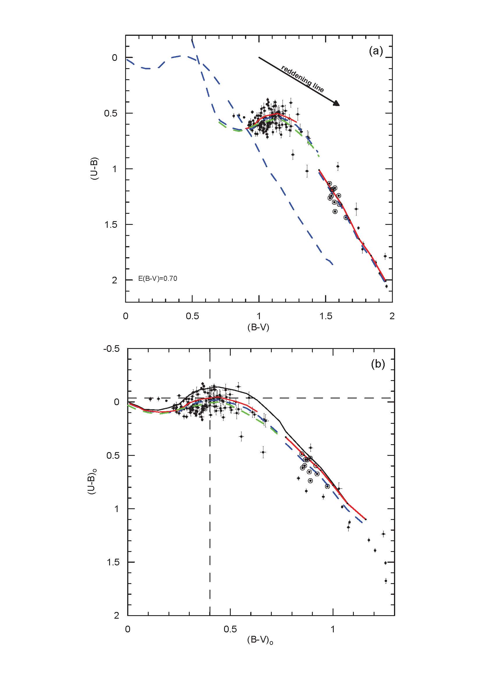
Figure 1: Shows the reddened, $(U$–$B,B$–$V)$, and the de-reddened, $((U$–$B)_{0},(B$–$V)_{0})$, diagrams for Ki 05. Panel (a): Blue dashed lines show the reddened and de-reddened SK82 relations for MS (upper section) and RG (lower section) stars. Panel (b): Green dashed and the upper solid black lines denote the Hyades main-sequence and the metal-free upper envelope of Melbourne (1959) and Sandage (1969), respectively. The red solid curve shows the estimated iso-metallicity line for [Fe/H]$=$$-$0.17 (Z =+0.013), as measured for this cluster; the vertical and horizontal lines show the mean values of $\langle(U$–$B)_{0}\rangle$ and $\langle(B$–$V)_{0}\rangle$ for F-type stars on the Ki 05 main sequence. A reddening vector is also shown as an arrow in panel (a). Big open circles mark the RC candidates.

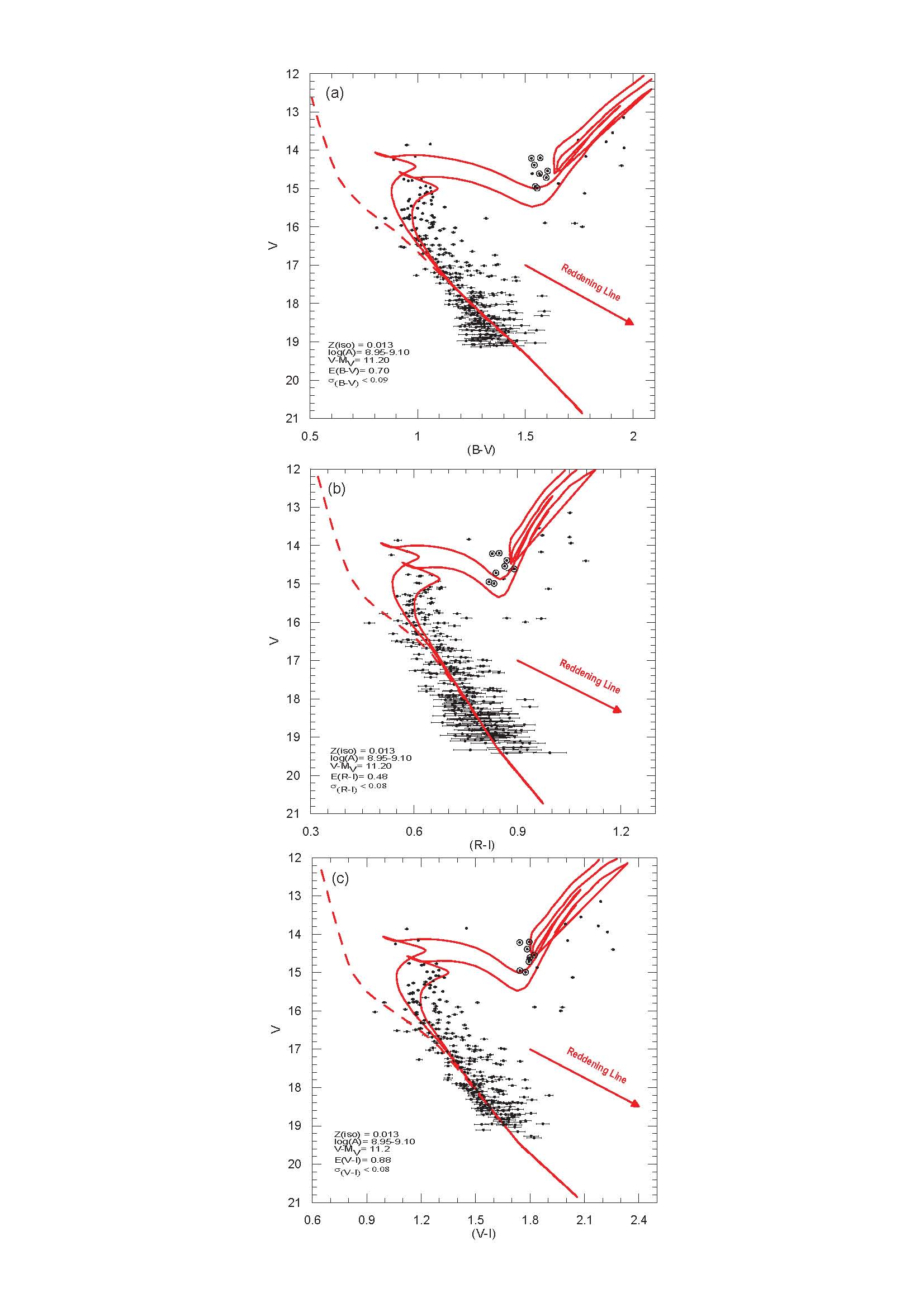
Figure 2: Panels (a)–(c): the CM diagrams of $(V,B$–$V)$, $(V,R$–$I)$, and $(V,V$–$I)$, respectively, for Ki 05. Solid lines show the M08 isochrones interpolated to $Z=+0.013$. Big open circles mark the RC candidates.

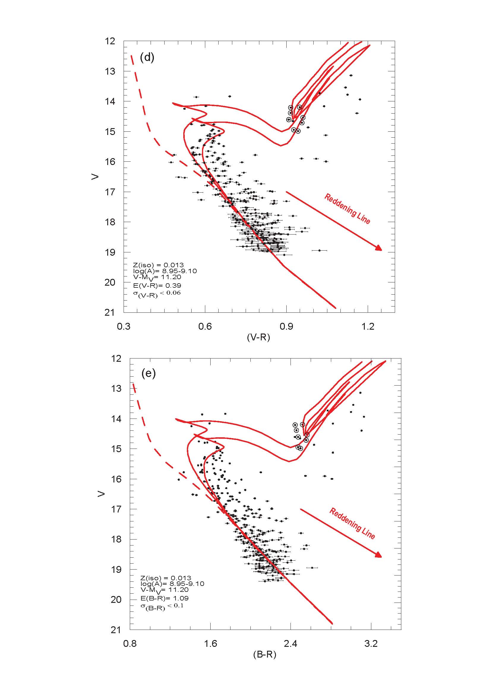
Figure 3: Panels (d)–(e): the CM diagrams of $(V,V$–$R)$ and $(V,B$–$R)$ for Ki 05. The symbols are the same as in Fig. 2.

Table 3: The values of $(B$–$V)$, $(U$–$B)_{H}$, $(U$–$B)_{M}$ for the Hyades main sequence (“H” suffix) and for approximately metal-free stars (“M”). The parts of the data of $(B$–$V)<0.35$ and $(B$–$V)>0.35$ are taken from Melbourne (1959) and Sandage (1969), respectively. $\delta(U$–$B)_{M}$ and $\delta_{0.6}/\delta_{M}$ in Columns 4 and 5 represent this maximum ultraviolet excess and the value needed to normalize this to $(B$–$V)=0.60$, respectively. Other normalization factors are available in table 1A of Sandage (1969) for lesser UV excesses.

$(B$–$V)$	$(U$–$B)_{H}$	$(U$–$B)_{M}$	$\delta(U$–$B)_{M}$	$\delta_{0.6}/\delta_{M}$
0.00	0.03	$+$0.01	0.02	15.5
0.05	0.08	$+$0.05	0.03	12.4
0.10	0.10	$+$0.08	0.03	12.4
0.15	0.11	$+$0.06	0.05	5.96
0.20	0.10	$+$0.00	0.10	3.10
0.25	0.07	$-$0.08	0.15	2.01
0.30	0.04	$-$0.17	0.21	1.46
0.35	0.03	$-$0.22	0.25	1.24
0.40	0.01	$-$0.25	0.26	1.19
0.45	0.00	$-$0.27	0.27	1.15
0.50	0.03	$-$0.25	0.28	1.11
0.55	0.08	$-$0.22	0.30	1.03
0.60	0.13	$-$0.18	0.31	1.00
0.65	0.19	$-$0.11	0.30	1.03
0.70	0.25	$-$0.03	0.28	1.10
0.75	0.34	$+$0.08	0.26	1.19
0.80	0.43	$+$0.19	0.24	1.29
0.85	0.54	$+$0.32	0.22	1.41
0.90	0.64	$+$0.44	0.20	1.55
0.95	0.74	$+$0.55	0.19	1.63
1.00	0.84	$+$0.67	0.17	1.82
1.05	0.94	$+$0.79	0.15	2.06
1.10	0.99	$+$0.87	0.12	2.58

4 Analyses of 20 O​Cs

Twenty O​Cs which contain F-type stars have been selected for the scope of this paper. Their selection has been based mostly on this presence of F-type stars, plus the fact that they have had limited previous attention in the literature; only about half of them have had previous metallicity determinations by photometric or spectroscopic methods. These O​Cs with F-type stars are quite valuable for photometric metal-abundance determination from the U–B, B–V plane in addition to providing interstellar reddenings, distances and photometric ages. However, our sample is rather small and may contain selection biases affecting the results of this paper. Moreover, our sample includes only a few O​Cs in each of the quadrants I, II, and III of the Galactic disc, the largest number in quadrant III, none in quadrant IV, and metal-poor old O​Cs are not well represented, as can be seen from Fig. 14. The majority of our cluster sample is located within $50^{o}$ of the Galactic anticentre direction.

Table 4: The mean values of $\langle(U$–$B)_{H}\rangle$ of the Hyades reference line, plus the mean $\langle(U$–$B)_{0}\rangle$ values, which correspond to the given $\langle(B$–$V)_{0}\rangle$ as set by the iso-abundance lines for the distributions in the (B–V) range (Col. 2) of F-type stars. The resulting ultraviolet excesses, $\delta(U$–$B)$, and their normalized values, $\delta_{0.6}$, plus their uncertainties (A10), are given in Columns 6 and 7, respectively. The number of dwarf stars in the F-star region is listed in the last column.

Cluster	(B-V) range	$\langle(B$–$V)_{0}\rangle$	$\langle(U$–$B)_{H}\rangle$	$\langle(U$–$B)_{0}\rangle$	$\delta(U$–$B)$	$\delta_{0.6}$	N
NGC 6694	(0.50$-$1.00)	0.39	0.010	$-$0.025	0.035	0.042$\pm 0.025$	58
NGC 6802	(0.90$-$1.20)	0.30	0.044	$-$0.010	0.054	0.079$\pm 0.020$	71
NGC 6866	(0.30$-$0.60)	0.44	0.000	$-$0.040	0.040	0.044$\pm 0.010$	36
NGC 7062	(0.70$-$1.10)	0.37	0.022	$-$0.044	0.066	0.080$\pm 0.015$	31
Ki 05	(0.90$-$1.30)	0.40	0.010	$-$0.036	0.046	0.058$\pm 0.040$	42
NGC 436	(0.50$-$1.10)	0.40	0.010	$-$0.090	0.100	0.119$\pm 0.050$	46
NGC 1798	(0.70$-$0.90)	0.31	0.041	$-$0.046	0.087	0.111$\pm 0.040$	41
NGC 1857	(0.60$-$0.90)	0.33	0.036	$-$0.034	0.070	0.088$\pm 0.030$	14
NGC 7142	(0.60$-$1.00)	0.50	0.030	$-$0.020	0.050	0.056$\pm 0.023$	40
Be 73	(0.50$-$0.70)	0.32	0.038	$-$0.012	0.050	0.064$\pm 0.010$	18
Haf 04	(0.50$-$0.90)	0.28	0.054	$+$0.004	0.050	0.084$\pm 0.030$	14
NGC 2215	(0.50$-$1.00)	0.37	0.022	$-$0.056	0.078	0.095$\pm 0.040$	37
Rup 01	(0.40$-$0.80)	0.38	0.018	$-$0.042	0.060	0.070$\pm 0.030$	14
Be 35	(0.40$-$0.80)	0.49	0.024	$-$0.025	0.049	0.052$\pm 0.030$	35
Be 37	(0.40$-$0.70)	0.40	0.010	$-$0.020	0.030	0.036$\pm 0.020$	52
Haf 08	(0.60$-$0.90)	0.44	0.000	$-$0.080	0.080	0.093$\pm 0.040$	34
Ki 23	(0.40$-$0.60)	0.44	0.000	$-$0.040	0.040	0.046$\pm 0.020$	18
NGC 2186	(0.50$-$1.00)	0.44	0.000	$-$0.080	0.080	0.093$\pm 0.030$	34
NGC 2304	(0.30$-$0.60)	0.37	0.002	$-$0.050	0.052	0.062$\pm 0.030$	23
NGC 2360	(0.30$-$0.60)	0.44	0.000	$-$0.040	0.040	0.046$\pm 0.020$	70

4.1 Interstellar reddenings and photometric metallicities

By following the analytic methods presented in detail in the works of T10 and A10, 20 O​Cs have been analysed in the two-colour (U–B, B–V) diagram and five CM diagrams together with the ZAMS intrinsic-colour calibrations of SK82, the Hyades main sequence colours of Sandage (1969) (Table 1A) and Melbourne (1959, 1960), and the Padova isochrones, Marigo et al. (2008, M08), to obtain reddenings, metallicities, distance moduli, and ages for these O​Cs.

As is presented in the works of T10 and A10, interstellar reddenings of the 20 O​Cs have been estimated from displacements of the intrinsic-colour sequences (dwarfs plus red giants) of SK82 in the CC diagram, as shown for Ki 05 in Fig. 1(a), until the best fit to the data of the clusters with an U–B shift of 0.72E(B–V)+0.05E(B–V)² and a (B–V) shift of E(B–V).

Photometric metal abundances [Fe/H] have been measured for F-type cluster stars in the CC diagram with respect to the Hyades mean main-sequence line, which is shown as dashed green lines in Figs. 1(a) and (b). Once the interstellar reddening shift has been made, the $\langle(U$–$B)_{0}\rangle$ and $\langle(B$–$V)_{0}\rangle$ colours have been fixed as mean values from the distribution of the F-type stars in each cluster. By using these $\langle(U$–$B)_{0}\rangle$ and $\langle(B$–$V)_{0}\rangle$ values, the iso-metallicity line (solid red line, Figs. 1(a) and (b)) as representative of the mean metal abundances of the cluster has been estimated, and these average values are given in Table 4 for the 20 O​Cs together with the data for the mean Hyades main sequence. From these $\langle(U$–$B)_{0}\rangle$ and $\langle(B$–$V)_{0}\rangle$ values of the 20 O​Cs, the values of $\delta(U$–$B)=(U$–$B)_{H}-\langle(U$–$B)_{0}\rangle$ have been measured, and normalized to $(B$–$V)_{0}=0.6$ via the data of Table 1A given by Sandage (1969). Then, the metallicity values, [Fe/H], for the 20 O​Cs have been derived from the empirical calibration, [Fe/H]–$\delta(U$–$B)_{0.6}$, as given in equation (6) of Karataş & Schuster (2006). These final [Fe/H] values are given for each cluster in Table 6.

Heavy-element abundances, $Z$, of the 20 O​Cs have been converted from the photometric metal abundances, [Fe/H], via the expression $Z=Z_{\odot}\cdot 10^{[Fe/H]}$. The solar abundance value has been taken as $Z_{\odot}=+0.019$, which is that adopted by M08 for their isochrones. However, Houdek & Gough (2011), Caffau et al. (2009), and Asplund et al. (2009) have published the values of $Z_{\odot}=+0.0142$, $+0.0156$, and $+0.0134$, respectively, based on helioseismology methods or spectroscopic chemical-composition analyses with 3D hydrodynamical solar models. A review of these and other solar values can be found in Asplund et al. (2009, Table 4). These lower solar metal abundances would have systematic effects on our results; for example, the isochrone ages would be systematically increased, and distances decreased.

Values of $\langle(B$–$V)_{0}\rangle$, $\langle(U$–$B)\rangle_{H}$, $\langle(U$–$B)_{0}\rangle$, $\delta(U$–$B)$, and $\delta_{0.6}$ have been given in Table 4 for the 20 O​Cs, and their [Fe/H] and $Z$ values are listed in Table 6. To be able to appreciate the photometric metal-abundance determination and the iso-metallicity line (the red curve in Fig. 1), Ki 05 has been taken as an example. The interstellar reddening value for this cluster has been measured as E(B–V)=0.70 mag by an appropriate shift in the CC diagram. The stars above the Hyades mean relation in the CC diagrams of Figs. 1(a) and (b) occupy the regions of $(B$–$V)\approx 0.9-1.3$, or $(B$–$V)_{0}\approx 0.20-0.60$, i.e. mostly F types. The mean values of the distribution correspond to $\langle(B$–$V)_{0}\rangle=0.40$ and $\langle(U$–$B)_{0}\rangle=-0.036$ for the F-type members of Ki 05. Then, $\delta(U$–$B)=(U$–$B)_{H}-\langle(U$–$B)_{0}\rangle=+0.01-(-0.036)=+0.046$, and $\delta_{0.6}/\delta(U$–$B)=1.19$ has been obtained via Table 1A. Finally, $\delta_{0.6}=+0.058$ is converted into $[Fe/H]=-0.17$ $(Z=+0.013)$ from the calibration of [Fe/H]–$\delta(U$–$B)_{0.6}$ of Karataş & Schuster (2006), who also have used the Hyades mean colours as reference. Thus, from the estimated values of $\langle(U$–$B)_{0}\rangle$ for $(B$–$V)_{0}\approx 0.24-0.44$, the iso-metallicity line which corresponds to $Z=+0.013$ has been drawn in Fig. 1 (the red curve).

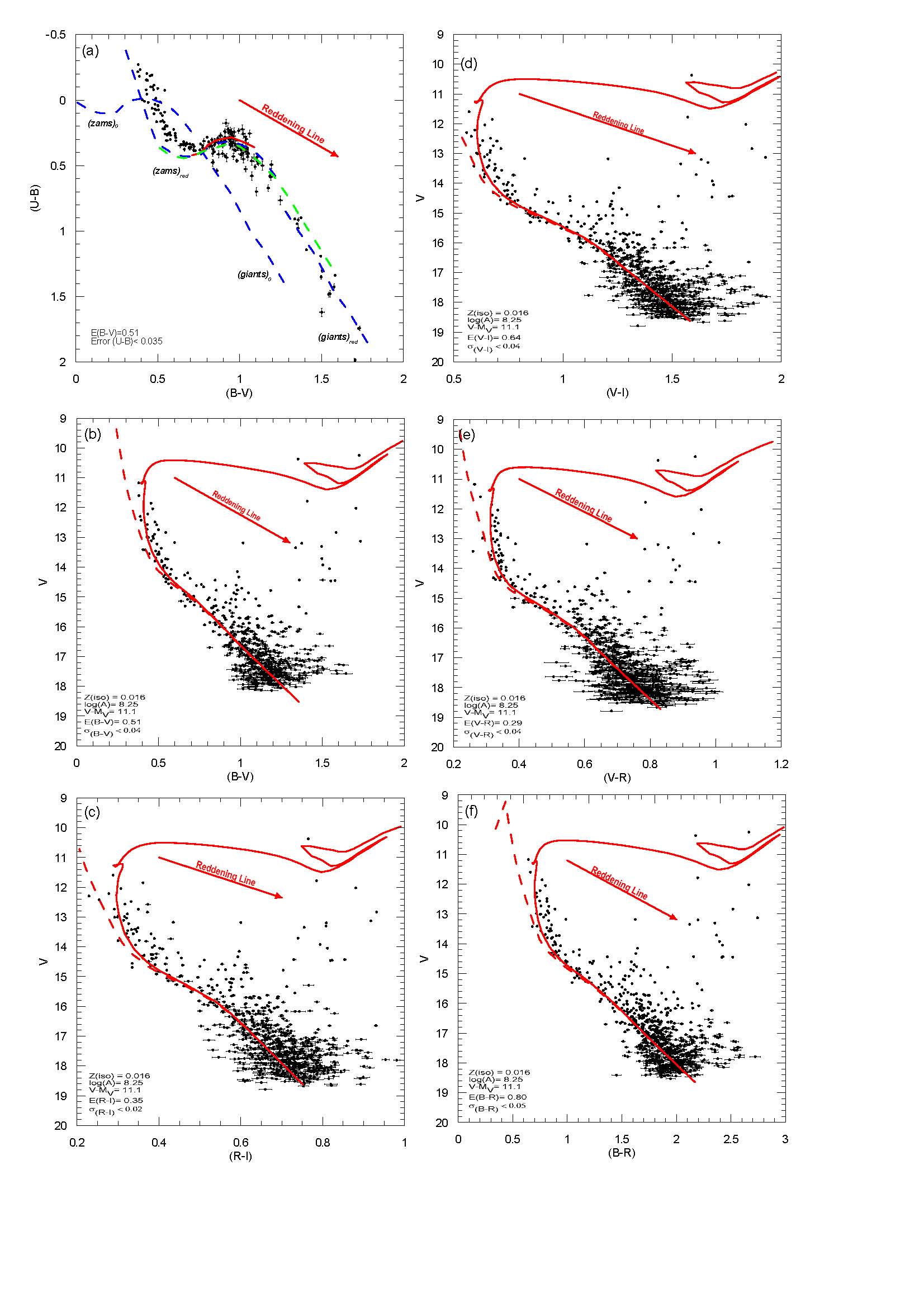
Figure S1: Panel (a): the $(U$–$B,B$–$V)$ diagram of NGC 6694. Panels (b)$-$(f): CM diagrams of $(V,B$–$V)$, $(V,R$–$I)$, $(V,V$–$I)$, $(V,V$–$R)$, and $(V,B$–$R)$. The symbols are the same as Fig. 1 and Figs. 2–3.

In addition, as is seen from the plots of the CM diagrams (Figs. 2-3 and Figs. S1-S19), O​Cs with RC/RG candidate stars are as follows: Ki 05, NGC 6802, NGC 6866, NGC 7062, NGC 1798, NGC 7142, Ru 01, Be 35, Be 37, Ki 23, NGC 2304, and NGC 2360. For these twelve O​Cs, to determine photometric metal abundances, the F-type stars in CC plots have been fit above the ZAMS colours of Hyades main sequence and simultaneously the RC/RG stars above the red-giant colours of SK82 with consistent ultraviolet excesses according to the normalizations of Sandage (1969). The best fit, the solid curve in CC diagrams, has the brightest bluer stars ($0.20<(B$–$V)_{0}<0.60$) slightly above the F-star hump of the Hyades main sequence, while the RC/RG stars ($0.90<(B$–$V)_{0}<1.30$) are slightly above the red-giant colours of SK82. The mean $(B$–$V)_{0}$ values and the numbers of F-type stars falling in their observed (B–V) range (Col. 2; Table 4) are given in Cols. 3 and 8 of Table 4, respectively. For the other eight O​Cs, for which RC/RG candidates are not clearly observed, only the F-type dwarf stars have been used for the metal abundance.

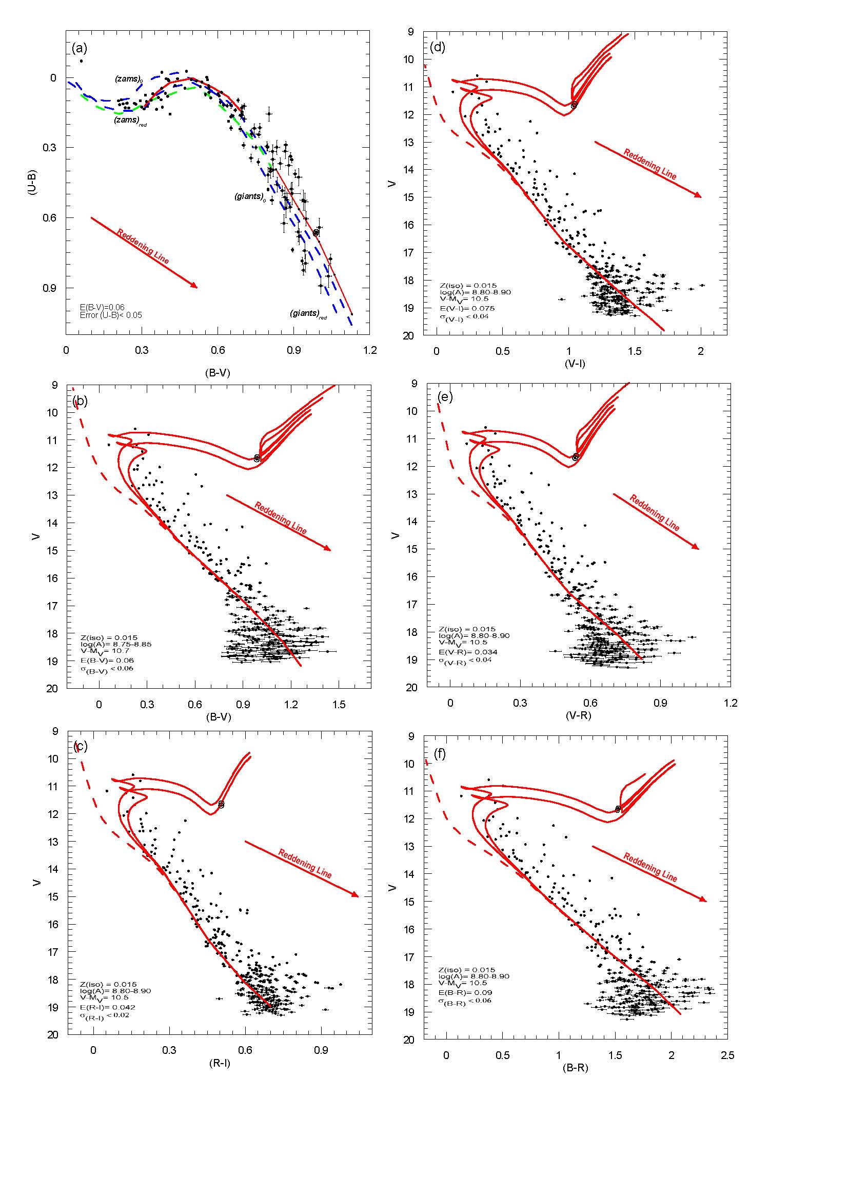
Figure S3: Panel (a): the $(U$–$B,B$–$V)$ diagram of NGC 6866. Panels (b)–(f): CM diagrams of $(V,B$–$V)$, $(V,R$–$I)$, $(V,V$–$I)$, $(V,V$–$R)$, and $(V,B$–$R)$. The symbols are the same as Fig. 1 and Figs. 2–3.

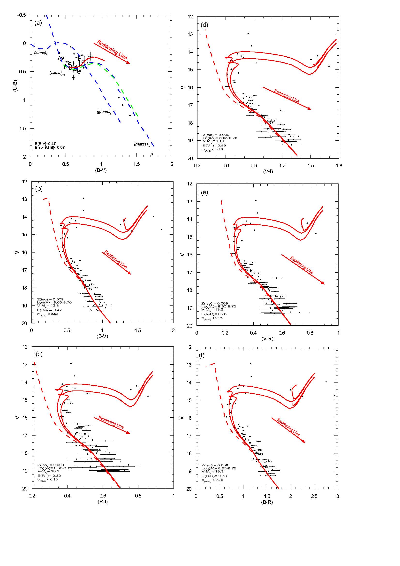
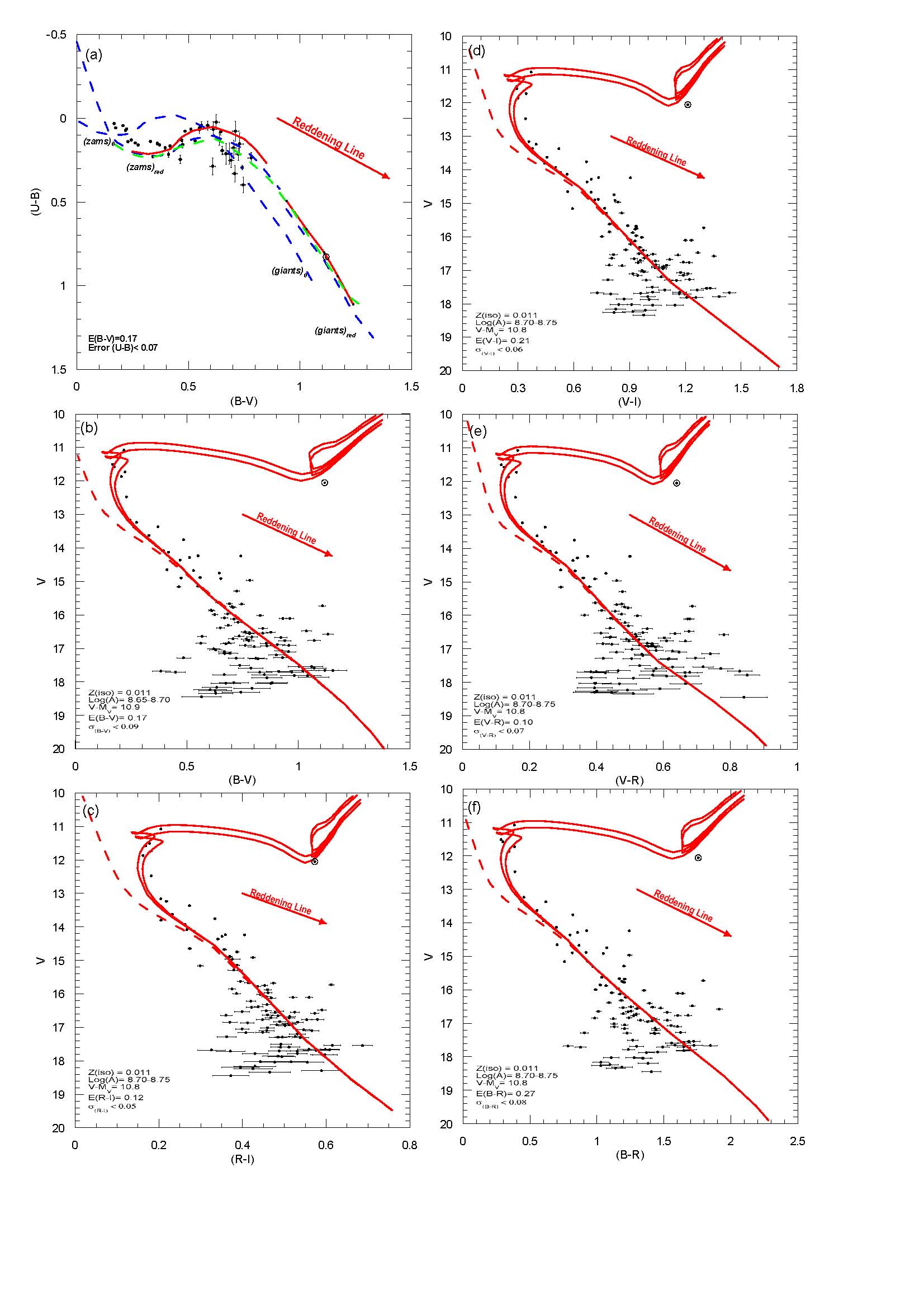
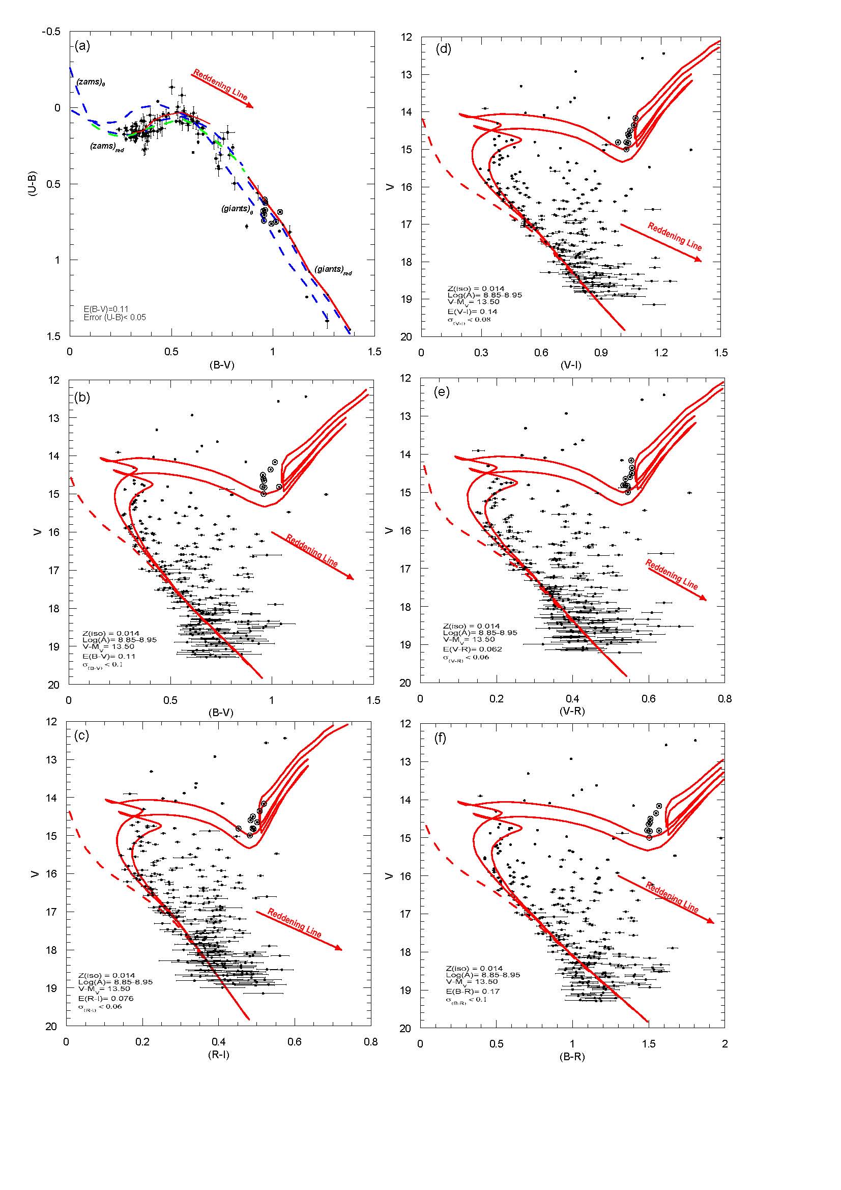
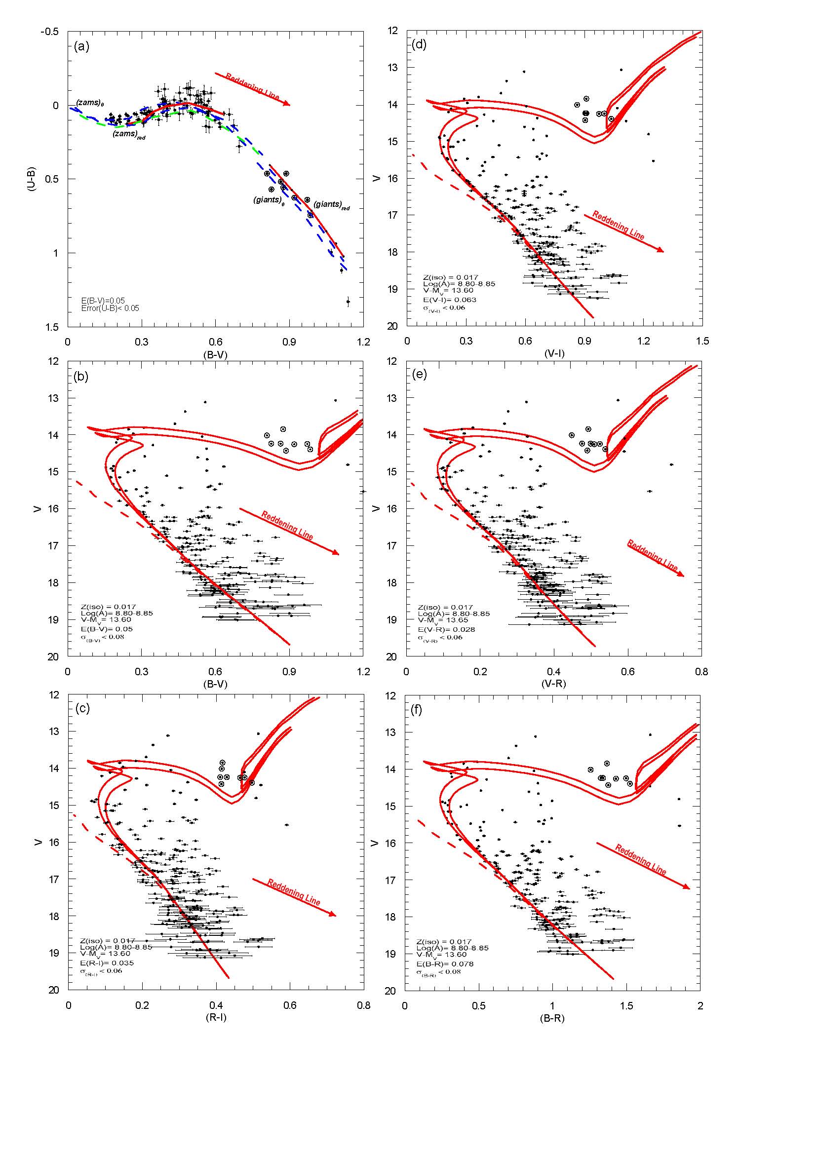
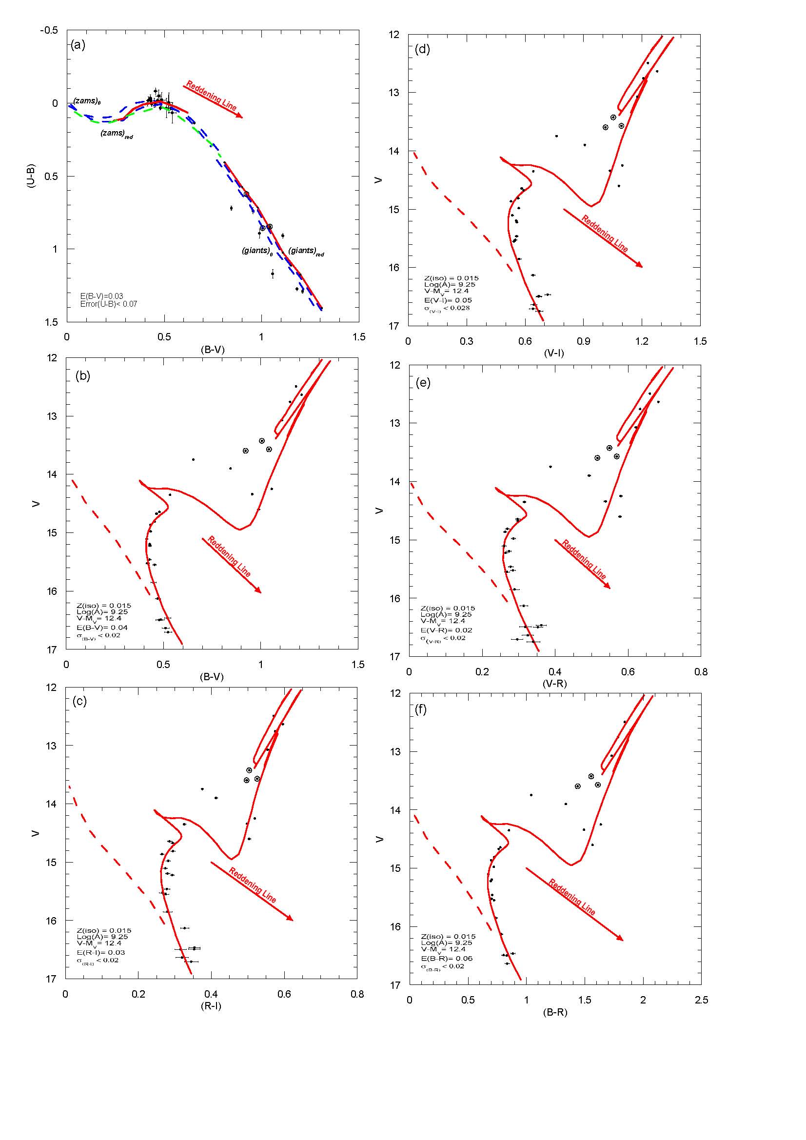
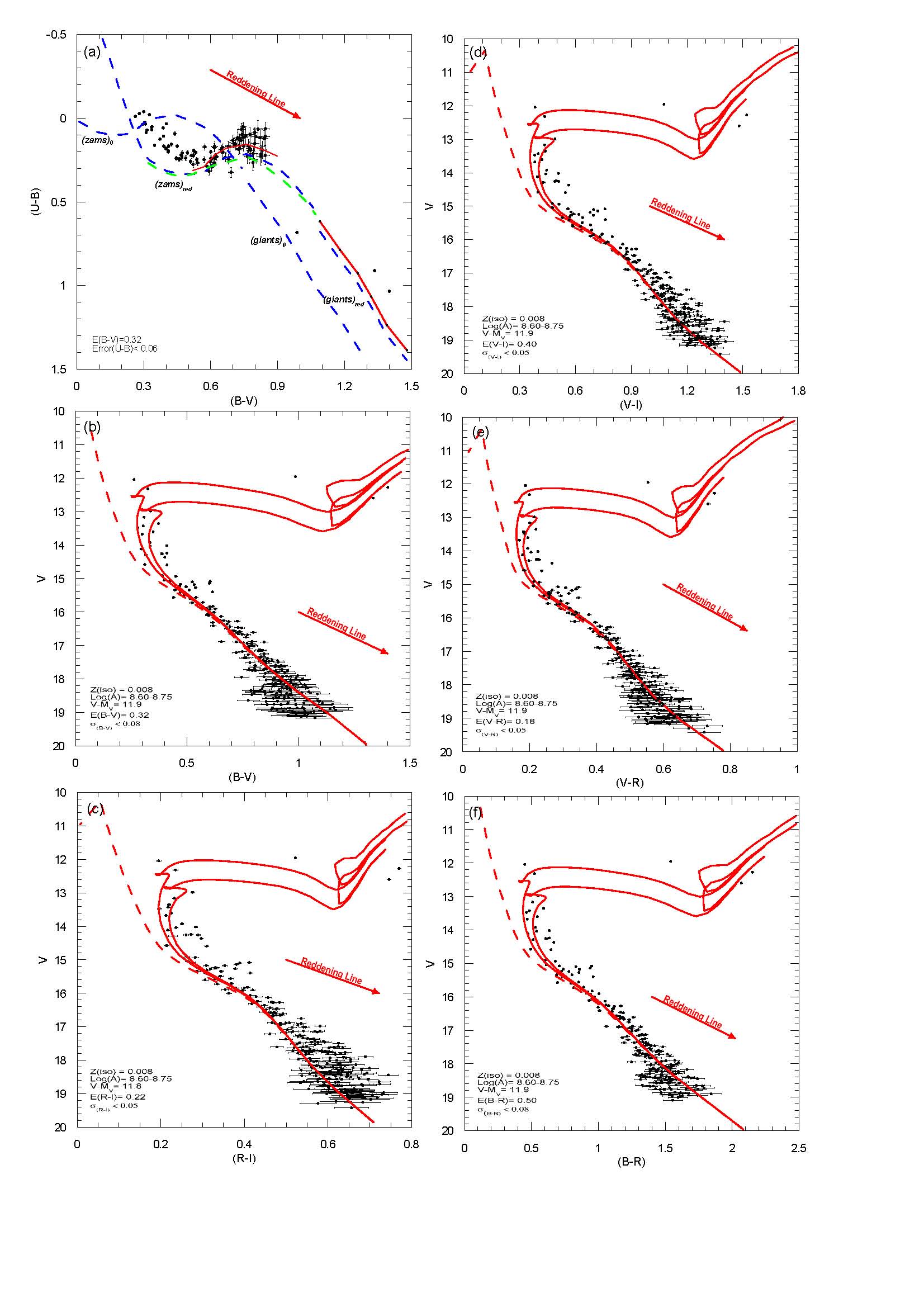
Figure S10: Panel (a): the $(U$–$B,B$–$V)$ diagram of Haf 04. Panels (b)–(f): CM diagrams of $(V,B$–$V)$, $(V,R$–$I)$, $(V,V$–$I)$, $(V,V$–$R)$, and $(V,B$–$R)$. The symbols are the same as Fig. 1 and Figs. 2–3.

Figure S11: Panel (a): the $(U$–$B,B$–$V)$ diagram of NGC 2215. Panels (b)–(f): CM diagrams of $(V,B$–$V)$, $(V,R$–$I)$, $(V,V$–$I)$, $(V,V$–$R)$, and $(V,B$–$R)$. The symbols are the same as Fig. 1 and Figs. 2–3.

Figure S12: Panel (a): the $(U$–$B,B$–$V)$ diagram of Rup 01. Panels (b)–(f): CM diagrams of $(V,B$–$V)$, $(V,R$–$I)$, $(V,V$–$I)$, $(V,V$–$R)$, and $(V,B$–$R)$. The symbols are the same as Fig. 1 and Figs. 2–3.

Figure S13: Panel (a): the $(U$–$B,B$–$V)$ diagram of Be 35. Panels (b)–(f): CM diagrams of $(V,B$–$V)$, $(V,R$–$I)$, $(V,V$–$I)$, $(V,V$–$R)$, and $(V,B$–$R)$. The symbols are the same as Fig. 1 and Figs. 2–3.

Figure S14: Panel (a): the $(U$–$B,B$–$V)$ diagram of Be 37. Panels (b)–(f): CM diagrams of $(V,B$–$V)$, $(V,R$–$I)$, $(V,V$–$I)$, $(V,V$–$R)$, and $(V,B$–$R)$. The symbols are the same as Fig. 1 and Figs. 2–3.

Figure S15: Panel (a): the $(U$–$B,B$–$V)$ diagram of Ki 23. Panels (b)–(f): CM diagrams of $(V,B$–$V)$, $(V,R$–$I)$, $(V,V$–$I)$, $(V,V$–$R)$, and $(V,B$–$R)$. The symbols are the same as Fig. 1 and Figs. 2–3.

The O​Cs: Ki 05, NGC 6802, NGC 7062, NGC 1798, NGC 7142, Be 35, Be 37, NGC 2304 and NGC 2360 show a clumpy distribution over $0.80<(B$–$V)_{0}<1.05$ in the CM diagrams, showing convincingly the presence of RC stars. On the other hand, Ki 23 shows a rather clear red-giant (RG) sequence in the CM diagrams (panels (b)–(f) of Figs. S15) with a few stars blueward of this RG branch which are also good RC candidates. NGC 6866 and Ru 01 (Figs. S3 and S12) show RC/RG stars which are probable good candidates for an RC star due to their position with respect to the isochrone. All of these RC stars have been emphasized with big open circles in the CC and CM diagrams due to their considerable usefulness as distance indicators.

4.2 Distances and Ages

The CM plots from the analysis of Ki 05 have been displayed in Figs. 2–3. The astrophysical parameters of Ki 05 are given in Table 5, and then summarized in Table 6 together with the fundamental astrophysical parameters for the other 19 O​Cs. The CC and CM diagrams, and the corresponding tables for the other 19 O​Cs have been presented as Tables S1–S4, and Figs. S1–S19 in the supplementary electronic section.

As is seen from Figs. 2(a)–(c) and 3(d)–(e) for Ki 05, the M08 isochrones, corresponding to the $Z$ value given in Table 4, have been over-plotted in five CM diagrams: $V,(B$–$V)$; $V,(R$–$I)$; $V,(V$–$I)$; $V,(V$–$R)$; and $V,(B$–$R)$, after reddening the isochrones along the colour axis with a colour excess corresponding to the $E(B$–$V)$ value given in Table 6, converted with help of the interstellar extinction ratios given in Table 6 of A10, and adding a visual extinction of $A_{\rm V}=3.1\times E(B$–$V)$ to the absolute magnitudes of the isochrones. The isochrones have then been shifted vertically to obtain the best fit to the observed intermediate section of the main sequence (MS), as well as the RC sequence. This vertical shift is the (true) distance modulus, $DM=(V_{0}$–$M_{\rm V})$. The average distance moduli and distances from the five CM diagrams for the 20 O​Cs have also been given in Table 6. To derive an age estimate for the clusters, the M08 isochrones, for the appropriate $Z$ values, have been shifted in the CM planes as above, i.e. $M_{V}+3.1E(B$–$V)+DM$ and $C_{0}(\lambda_{1}-\lambda_{2})+E[C(\lambda_{1}-\lambda_{2})]$, respectively, and then the isochrone ages have been varied until a satisfactory fit to the data has been obtained through the observed upper MS, TO, and RC sequences. The resulting average inferred mean ages are presented in Table 6, Col. 8.

For most of these CM diagrams, two isochrones have been plotted to provide a means for appreciating the uncertainties of the derived distances and ages. In Column 4 of Table 5 and of Tables S1-S4 (see the supplementary section), the range in ages provided by these isochrone pairs is given. The final mean values for the distances and ages from the five CM diagrams are given in the final line for each cluster in these tables; the error estimates and the calculation of the weighted mean values of E(B–V), [Fe/H], $(V_{0}$–$M_{\rm V})$, $d$ (kpc), log(A), and A have been calculated as described in Sect. 3.4 of A10. For the parameters, $(V_{0}$–$M_{\rm V})$, $d$ (kpc), and log(A), the mean values and the associated mean uncertainty have been calculated from the individual uncertainties of the five CM diagrams, weighted with their respective precisions, using the expressions (8)–(9) given in A10. These errors take into account an attempt to estimate external errors, as in A10, since the photometric indices and the five resulting CM diagrams are not independent.

Table 5: The derived fundamental astrophysical parameters of Ki 05.

Colour	$(V_{0}$–$M_{V})$	d (kpc)	log(A)-range	log(A)	A (Gyr)
$E(B$–$V)=0.70\pm 0.08$, $[Fe/H]=-0.17\pm 0.25$, $Z=0.013\pm 0.007$
$(B$–$V)$	11.20$\pm$0.12	1.74$\pm$0.09	8.95$-$9.10	9.10$\pm$0.10	1.26$\pm$0.33
$(R$–$I)$	11.20$\pm$0.20	1.74$\pm$0.16	8.95$-$9.10	9.10$\pm$0.15	1.26$\pm$0.52
$(V$–$I)$	11.20$\pm$0.10	1.74$\pm$0.08	8.95$-$9.10	9.10$\pm$0.10	1.26$\pm$0.33
$(V$–$R)$	11.20$\pm$0.10	1.74$\pm$0.08	8.95$-$9.10	9.10$\pm$0.10	1.26$\pm$0.33
$(B$–$R)$	11.20$\pm$0.10	1.74$\pm$0.08	8.95$-$9.10	9.10$\pm$0.10	1.26$\pm$0.33
Mean	11.20$\pm$0.05	1.74$\pm$0.04		9.10$\pm$0.05	1.26$\pm$0.16

Table 6: The fundamental astrophysical parameters of the 20 O​Cs. Galactic coordinates have been taken from the WEBDA data-base.

Cluster	$\textit{l}^{\circ}$	$b^{\circ}$	E(B–V)	[Fe/H]	Z	$(V_{0}$–$M_{V})$	A(Gyr)	d (kpc)
NGC6694	23.88	$-$2.91	0.51$\pm$0.06	$-0.09\pm 0.14$	0.016$\pm$ 0.005	11.10$\pm$0.04	0.18$\pm$0.01	1.66$\pm$0.03
NGC6802	55.34	$+$0.92	0.80$\pm$0.07	$-0.30\pm 0.13$	0.009$\pm$ 0.003	11.19$\pm$0.05	1.12$\pm$0.08	1.73$\pm$0.04
NGC6866	79.56	$+$6.84	0.06$\pm$0.05	$-0.10\pm 0.05$	0.015$\pm$ 0.002	10.61$\pm$0.02	0.75$\pm$0.04	1.32$\pm$0.01
NGC7062	89.96	$-$2.75	0.43$\pm$0.08	$-0.31\pm 0.09$	0.010$\pm$ 0.002	11.40$\pm$0.02	0.71$\pm$0.04	1.91$\pm$0.02
Ki05	143.78	$-$4.29	0.70$\pm$0.08	$-0.17\pm 0.25$	0.013$\pm$ 0.007	11.20$\pm$0.05	1.26$\pm$0.16	1.74$\pm$0.04
NGC436	126.11	$-$3.91	0.40$\pm$0.07	$-0.55\pm 0.33$	0.005$\pm$ 0.004	11.90$\pm$0.05	0.18$\pm$0.03	2.40$\pm$0.05
NGC1798	160.70	$+$4.85	0.47$\pm$0.07	$-0.50\pm 0.28$	0.006$\pm$ 0.004	12.70$\pm$0.04	1.78$\pm$0.22	3.47$\pm$0.06
NGC1857	168.40	$+$1.26	0.47$\pm$0.08	$-0.36\pm 0.19$	0.008$\pm$ 0.003	11.98$\pm$0.04	0.32$\pm$0.04	2.49$\pm$0.05
NGC7142	105.35	$+$9.48	0.35$\pm$0.08	$-0.16\pm 0.12$	0.013$\pm$ 0.004	11.60$\pm$0.05	3.55$\pm$0.57	2.10$\pm$0.05
Be 73	215.28	$-$9.42	0.28$\pm$0.06	$-0.21\pm 0.06$	0.012$\pm$ 0.002	14.50$\pm$0.03	1.41$\pm$0.08	7.93$\pm$0.11
Haf 04	227.94	$-$3.59	0.47$\pm$0.09	$-0.33\pm 0.19$	0.009$\pm$ 0.008	13.22$\pm$0.05	0.42$\pm$0.05	4.39$\pm$0.10
NGC 2215	215.99	$-$10.10	0.23$\pm$0.07	$-0.40\pm 0.27$	0.008$\pm$ 0.005	9.60$\pm$0.03	0.64$\pm$0.05	0.83$\pm$0.01
Rup 01	223.99	$-$9.69	0.17$\pm$0.06	$-0.25\pm 0.18$	0.011$\pm$ 0.005	10.85$\pm$0.04	0.48$\pm$0.04	1.48$\pm$0.03
Be 35	212.60	$+$5.35	0.11$\pm$0.07	$-0.13\pm 0.18$	0.014$\pm$ 0.006	13.50$\pm$0.04	0.89$\pm$0.06	5.01$\pm$0.10
Be 37	217.23	$+$5.94	0.05$\pm$0.05	$-0.05\pm 0.08$	0.017$\pm$ 0.003	13.60$\pm$0.02	0.63$\pm$0.06	5.25$\pm$0.06
Haf 08	227.53	$+$1.34	0.32$\pm$0.07	$-0.39\pm 0.26$	0.008$\pm$ 0.005	11.88$\pm$0.04	0.56$\pm$0.07	2.38$\pm$0.04
Ki 23	215.53	$+$7.20	0.03$\pm$0.02	$-0.11\pm 0.11$	0.015$\pm$ 0.004	12.40$\pm$0.02	1.78$\pm$0.07	3.02$\pm$0.03
NGC 2186	203.54	$-$6.19	0.26$\pm$0.07	$-0.39\pm 0.26$	0.008$\pm$ 0.005	11.40$\pm$0.03	0.32$\pm$0.04	1.91$\pm$0.03
NGC 2304	197.21	$+$8.90	0.03$\pm$0.03	$-0.20\pm 0.18$	0.012$\pm$ 0.005	12.79$\pm$0.02	0.93$\pm$0.03	3.61$\pm$0.03
NGC 2360	229.81	$-$1.42	0.01$\pm$0.07	$-0.11\pm 0.11$	0.015$\pm$ 0.004	10.25$\pm$0.02	1.12$\pm$0.07	1.12$\pm$0.01

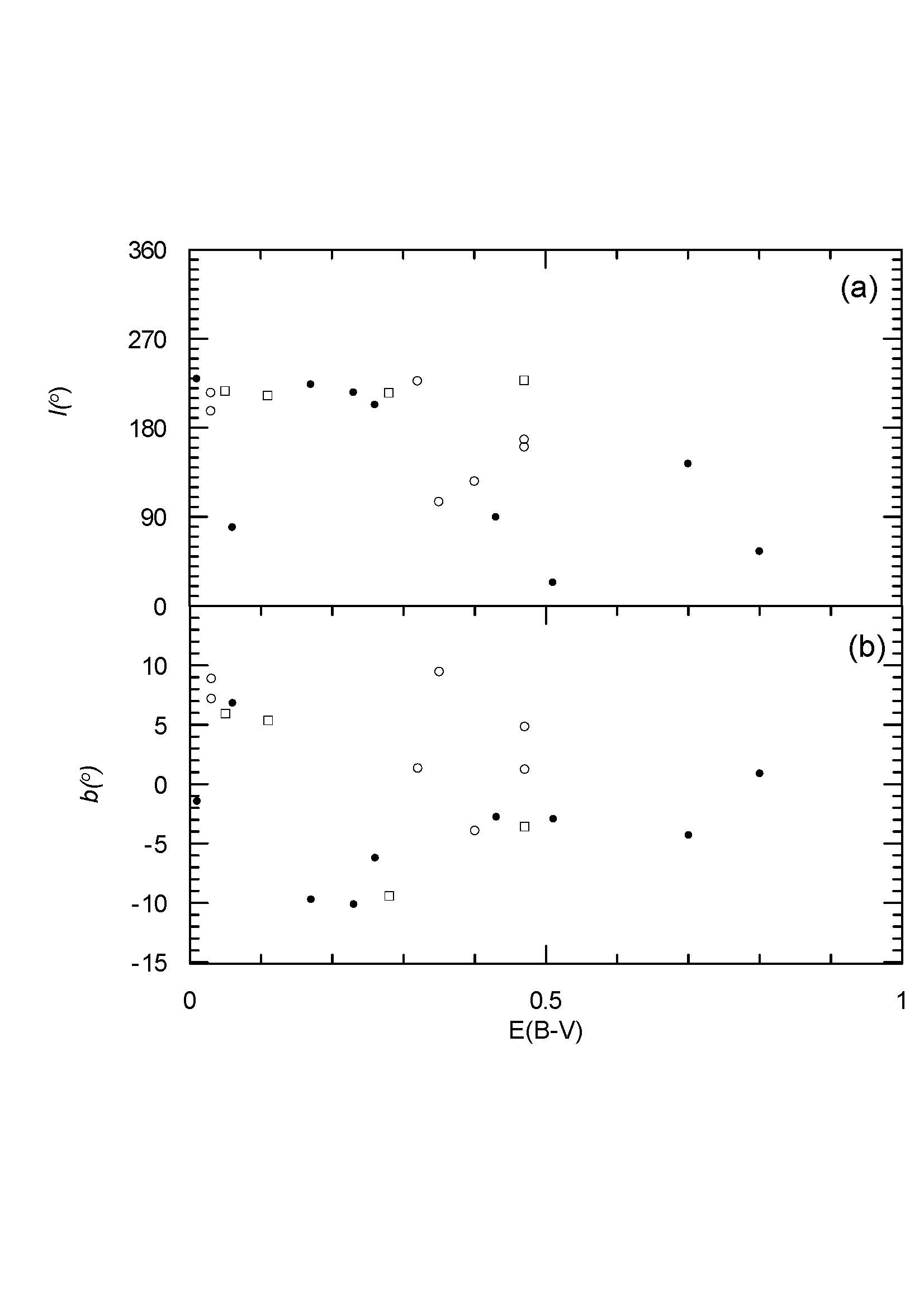
Figure 4: (a) $E(B$-$V)$ versus $\textit{l}^{\circ}$ and (b) versus $\textit{b}^{\circ}$. Filled and open circles show the O​Cs with d = [0, 2] kpc and d = [2, 4] kpc, respectively, while open squares represent those with d $>$ 4 kpc

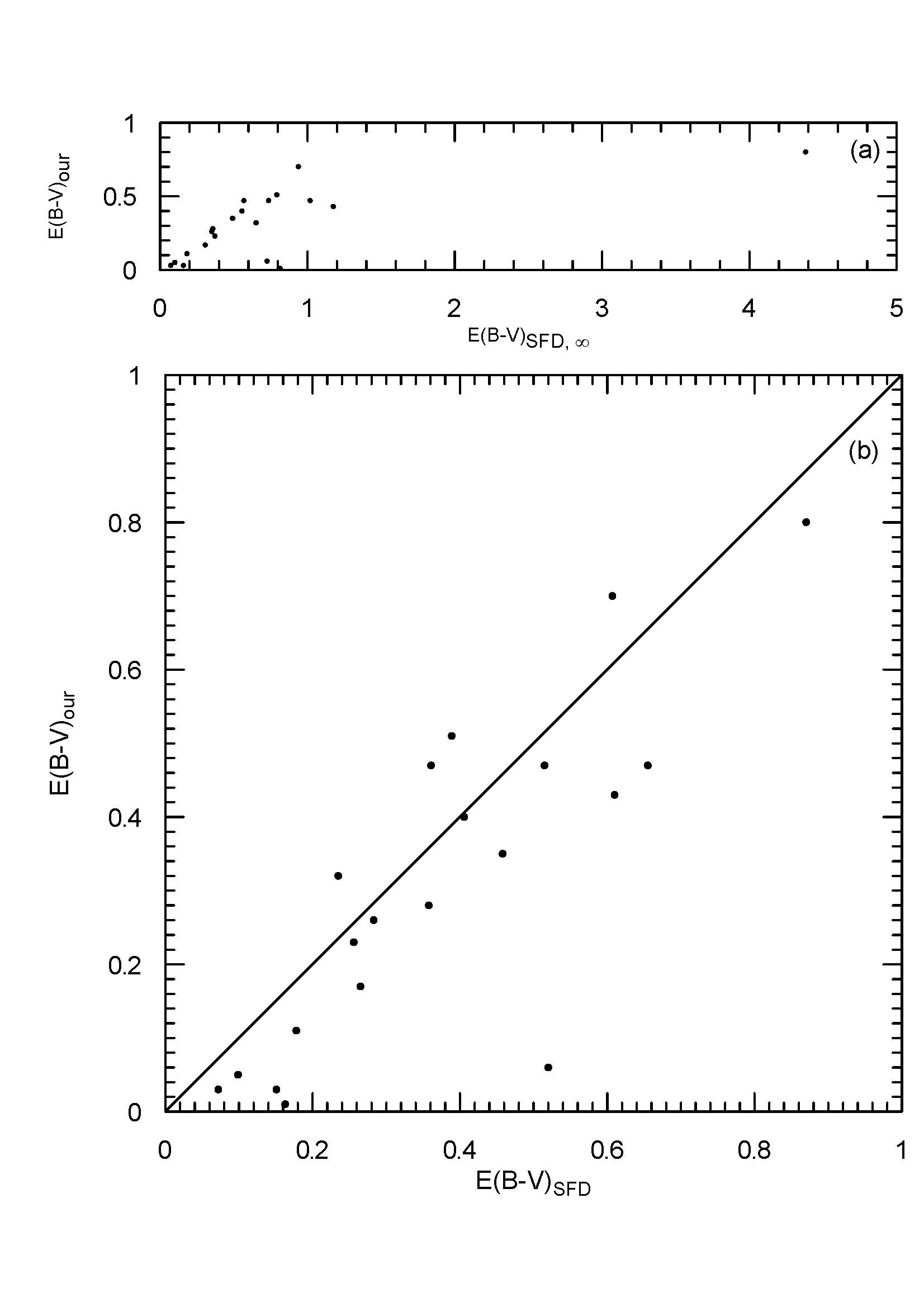
Figure 5: (a) $E(B$–$V)_{\rm SFD,\infty}$ versus $E(B$–$V)$, and (b) $E(B$–$V)_{\rm SFD}$ versus $E(B$–$V)$.

4.3 Correlations of the Interstellar Reddenings

The $E(B$–$V)$ versus Galactic longitude ($\textit{l}^{\circ}$) and latitude ($\textit{b}^{\circ}$) plots, as a function of the cluster distances, have been given in Figs. 4(a) and (b), respectively, where filled and open circles show the $d=[0,~{}2]$ kpc and $d=[2,~{}4]$ kpc subsets, respectively; open squares represent those with $d>4$ kpc. As is seen from panel (a), except for Ki 05 with E(B$-$V)=0.70 and l=143${}^{\circ}.78$, the reddenings of the O​Cs in the anticentre directions have $E(B$–$V)<0.50$; the distances of these O​Cs fall in the range $0<d<8$ kpc. There are two O​Cs with $E(B$–$V)>0.50$ in the Galactic centre direction, and the distances of clusters in quadrant I are less than 2 kpc. The distribution of $E(B$–$V)$–$\textit{l}^{\circ}$ in Fig. 4(a) is in quite good agreement with the one of Joshii (2005, fig. 6). It is seen from panel (b) that the O​Cs fall in the range of $-10^{\circ}$ $\leq$ b $\leq$ $+10^{\circ}$. O​Cs with $|b|$ $>$ $5^{\circ}$ have $E(B$–$V)$ $<$ $0.40$, whereas the O​Cs inside $|b|$$<$$5^{\circ}$ fall in the range $0.30<E(B$–$V)<0.80$.

The $E(B$–$V)$ values from extinction maps given by Schlegel et al. (1998, hereafter SFD) (based on the IRAS 100-micrometer surface brightness converted to extinction) have been compared with our values. The relations of $E(B$–$V)_{\rm SFD,\infty}$ versus $E(B$–$V)$, and $E(B$–$V)_{\rm SFD}$ versus $E(B$–$V)$ of the 20 O​Cs are displayed in Figs. 5(a) and (b), respectively. It is seen from Fig. 5(a) that there is a large discrepancy between the $E(B$–$V)$ values for five O​Cs, with the $E(B$–$V)_{\rm SFD,\infty}$ values being much larger than ours. For a correction of the SFD reddening estimates, the equations of Bonifacio et al. (2000) and Schuster et al. (2004) have been adopted. Then the final reddening, $E(B$–$V)_{\rm SFD}$, for a given star is reduced compared to the total reddening $E(B$–$V)(\ell,b)_{\infty}$ by a factor $\{1-\exp[-d\sin|b|/H]\}$, given by Bahcall & Soneira (1980), where $b$, $d$, and $H$ are the Galactic latitude (Column 3 of Table 6), the distance from the observer to the object (Column 9 of Table 6), and the scale height of the dust layer in the Galaxy, respectively; here we have assumed $H=125$ pc (Bonifacio et al., 2000). Note that Galactic latitudes of our O​Cs are less than $10^{\circ}$. These reduced final reddenings have been compared with our measured ones in Fig. 5(b). The differences in $\Delta E(B$–$V)$ in Fig. 5(b) are at the level of 0.11–0.46 for eight O​Cs between corresponding $E(B$–$V)$ values. For the rest, the $E(B$–$V)$ values of the clusters are in fairly good concordance with the ones of SFD. However, as discussed by Chen et al. (1999), from samples of open and globular clusters at $|b|>2.5^{\circ}$, the SFD reddening values tend to overestimate $E(B$–$V)$ by a factor of up to 1.16–1.18. Arce & Goodman (1999), Cambresy et al. (2005), and Joshii (2005) have also confirmed that SFD maps overestimate the extinction in several parts of the sky. (The corrections of Bonifacio et al. (2000) and Schuster et al. (2004) have been derived from such studies.) According to Cambresy et al. (2005), the reason is due to the presence of fluffy/composite grains leading to an enhanced far-infrared emissivity.

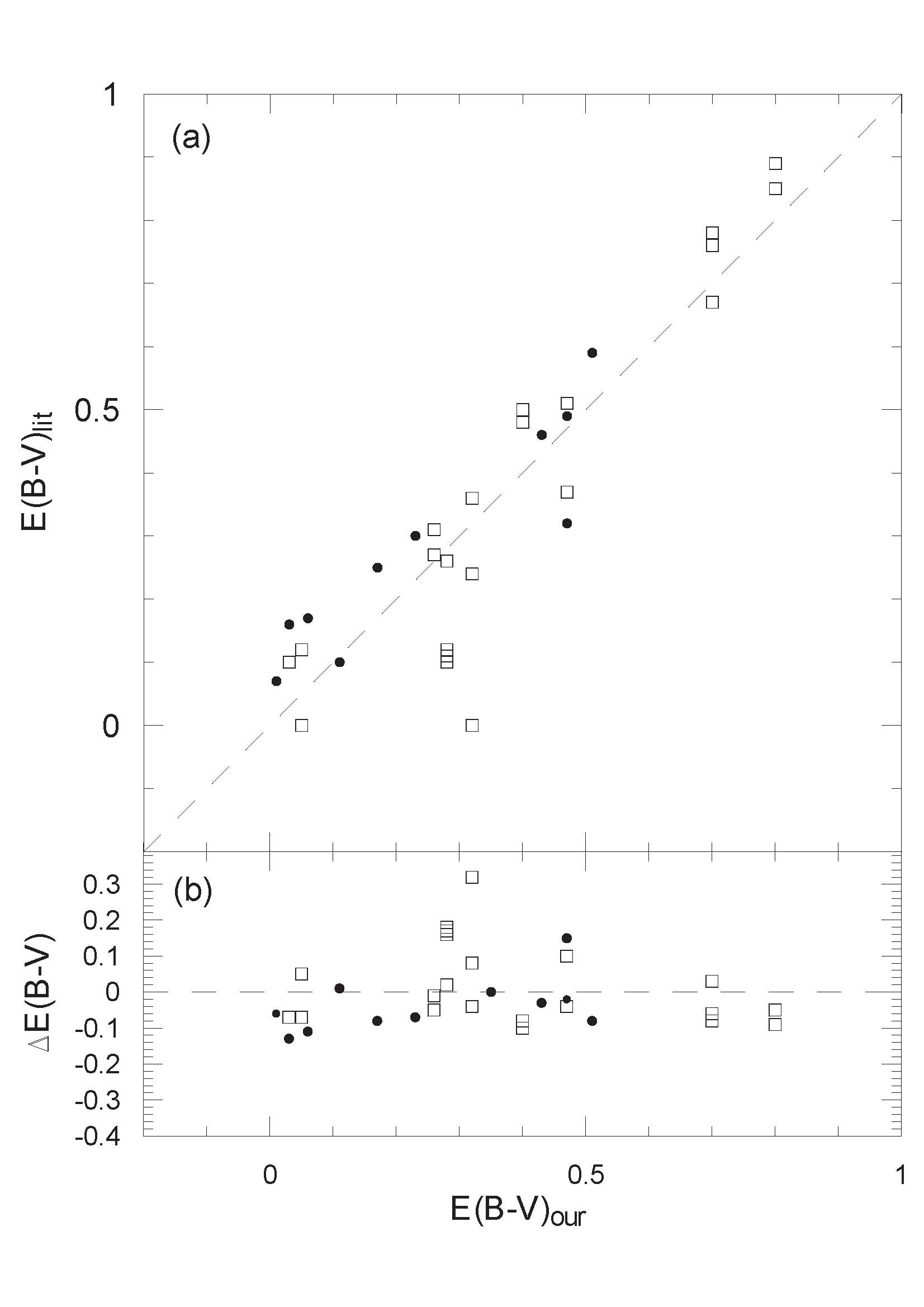
Figure 6: Comparison of our $E(B$–$V)$’s with ones from the literature. Filled circles represent O​Cs with only one literature value, whereas open squares show ones with more than one literature value. Panel (b) shows differences between our values and those of the literature, $\Delta E(B$–$V)=E(B$–$V)_{\rm our}-E(B$–$V)_{\rm lit}$.

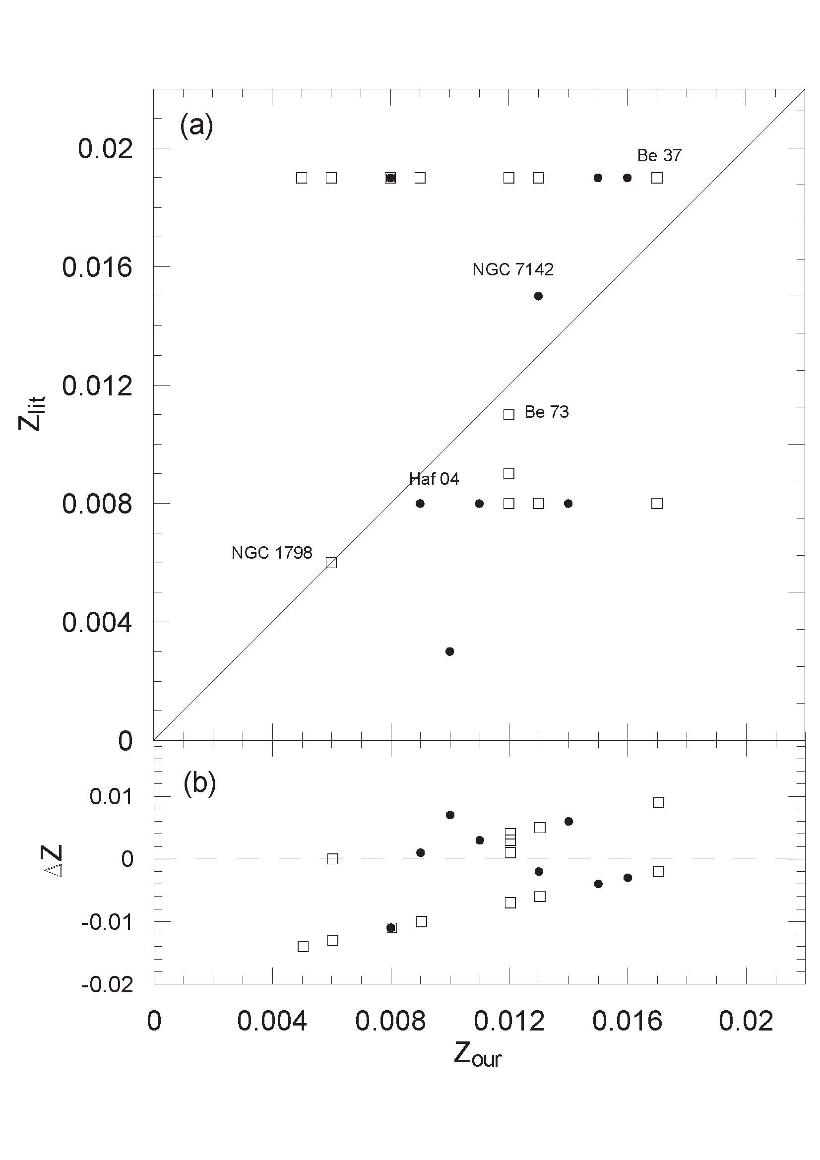
Figure 7: Comparison of the mass-fraction heavy-element abundances, $Z$, with values from the literature. Again, panel (b) shows our differences with respect to the literature as a function of $Z_{\rm our}$, $\Delta Z=Z_{\rm our}-Z_{\rm lit}$. The symbols are the same as in Fig. 6.

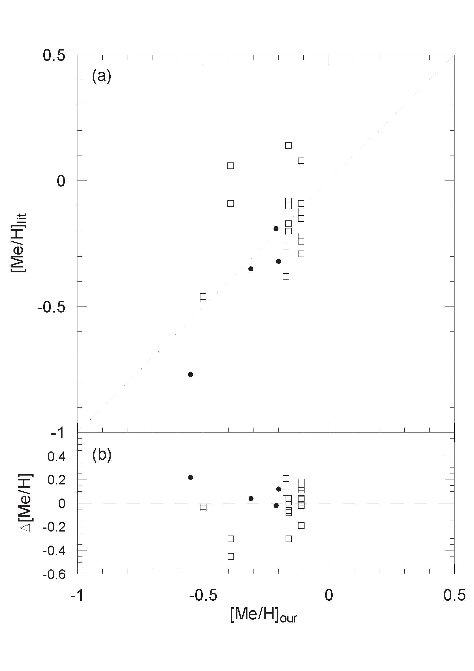
Figure 8: Comparison of the logarithmic metal abundances, [Me/H], of nine O​Cs with values from the literature. The symbols and panels are the same as in Fig. 6.

Figure 9: Comparison of our distance moduli with ones from the literature. The symbols and panels as in Fig. 6.

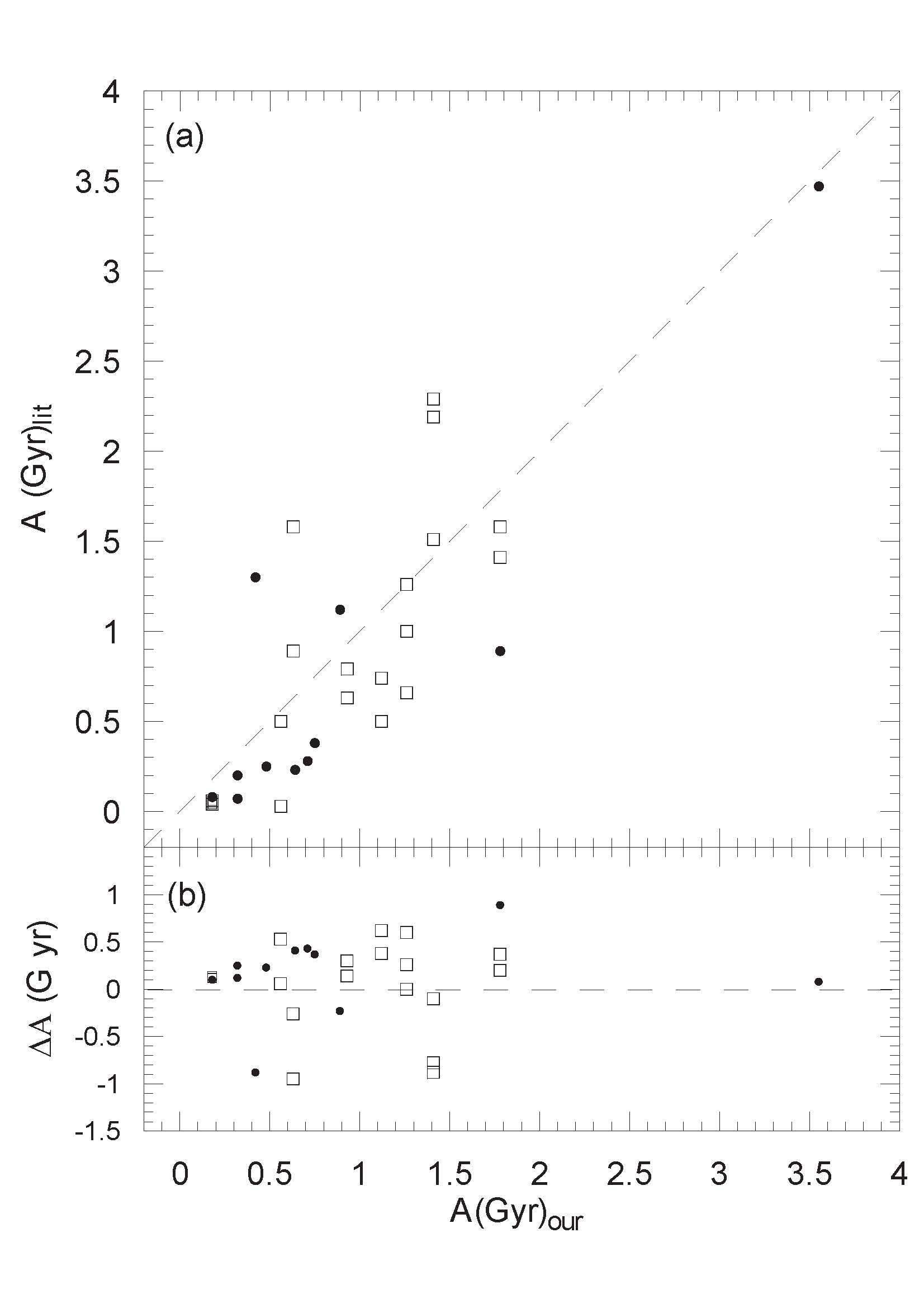
Figure 10: Comparison of our ages with ones from the literature. The symbols and panels as in Fig. 6.

Table 7: The comparisons of reddenings, heavy-element abundances, distance moduli/distances, and ages of the 20 O​Cs. Columns (2)–(6) show the values of this work, and Columns (7)–(12) the values from the literature. In Column (9) ZAMS/OMS indicates whether a ZAMS from either isochrones or from an observational main sequences (OMS) has been used in the literature. References for the data in Columns 7–12 are listed in the last column.

Cluster	$E(B$–$V)$	Z	$(V_{0}$–$M_{V})$	d (kpc)	A (Gyr)	$E(B$-$V)$	$Z$	ZAMS/OMS	$(V_{0}$–$M_{V})$	d (kpc)	A(Gyr)	References
NGC 6694	0.51	0.016	11.10	1.66	0.18	0.59	0.019	OMS	10.00	1.00	0.08	1
NGC 6802	0.80	0.009	11.19	1.73	1.12	0.85	0.019	OMS	10.34	1.17	0.74	2
						0.89	0.019	Claret et al. 2003; ZAMS	11.64	2.13	0.50	3
NGC 6866	0.06	0.015	10.61	1.32	0.75	0.17	0.019	OMS	10.80	1.45	0.38	2
NGC 7062	0.43	0.010	11.40	1.91	0.71	0.46	0.003	Vandenberg 1985; ZAMS	12.18	2.73	0.28	4
Ki 05	0.70	0.013	11.20	1.74	1.26	0.67	0.019	Bertelli et al. 1994; ZAMS	11.74	2.23	1.26	5
						0.78	0.008	Vandenberg 1985; ZAMS	11.40	1.90	1.00	6
						0.76	0.008	Bertelli et al. 1994; ZAMS	11.40	1.90	0.66	7
NGC 436	0.40	0.005	11.90	2.40	0.18	0.48	0.019	Bertelli et al. 1994; ZAMS	12.34	2.94	0.06	8
						0.50	0.019	Maeder and Meynet 1991; ZAMS	12.55	3.24	0.04	9
						0.48	0.019	Maeder and Meynet 1989; ZAMS	12.06	2.58	0.06	10
NGC 1798	0.47	0.006	12.70	3.47	1.78	0.37	0.019	Bertelli et al. 1994; ZAMS	12.75	3.55	1.58	11
						0.51	0.006	Bertelli et al. 1994; ZAMS	13.10	4.17	1.41	12
NGC 1857	0.47	0.008	11.98	2.49	0.32	0.49	0.019	Barbaro et al. 1969; ZAMS	13.15	4.27	0.07	13
NGC 7142	0.35	0.013	11.60	2.10	3.55	0.35	0.015	Mermilliod 1981; ZAMS	11.40	1.91	3.47	14
Be 73	0.28	0.012	14.50	7.93	1.41	0.10	0.008	Bertelli et al. 1994; ZAMS	14.20	6.92	2.29	15
						0.12	0.008	Girardi et al. 2000; ZAMS	14.93	9.68	1.51	16
						0.11	0.011	Girardi et al. 2000; ZAMS	14.93	9.68	1.51	17
						0.26	0.008	Bertelli et al. 1994; ZAMS	14.63	8.43	2.19	18
Haf 04	0.47	0.009	13.22	4.39	0.42	0.32	0.008	Bertelli et al. 1994; ZAMS	13.16	4.29	1.30	18
NGC 2215	0.23	0.008	9.60	0.83	0.64	0.30	0.019	OMS	9.63	0.84	0.23	19
Rup 01	0.17	0.011	10.85	1.48	0.48	0.25	0.008	Girardi et al. 2002; ZAMS	10.88	1.50	0.25	20
Be 35	0.11	0.014	13.50	5.01	0.89	0.10	0.008	Bertelli et al. 1994; ZAMS	13.82	5.81	1.12	18
Be 37	0.05	0.017	13.60	5.25	0.63	0.00	0.008	Bertelli et al. 1994; ZAMS	13.75	5.62	1.58	18
						0.12	0.019	Bonatto et al. 2004; ZAMS	13.40	4.79	0.89	21
Haf 08	0.32	0.008	11.88	2.38	0.56	0.00	0.019	SK65; OMS	11.10	1.66	0.03	22
						0.36	0.019	SK65; OMS	11.04	1.61	-	23
						0.24	0.019	Girardi et al. 2000; ZAMS	12.07	2.59	0.50	17
Ki 23	0.03	0.015	12.40	3.02	1.78	0.16	0.019	Bonatto et al. 2004; ZAMS	12.60	3.31	0.89	21
NGC 2186	0.26	0.008	11.40	1.91	0.32	0.31	0.019	SK65; OMS	11.31	1.83	-	23
						0.27	0.019	Girardi et al. 2002; ZAMS	12.16	2.70	0.20	24
NGC 2304	0.03	0.012	12.79	3.61	0.93	0.10	0.009	Bertelli et al. 1994; ZAMS	13.00	3.98	0.79	25
						0.10	0.019	Girardi et al. 2002; ZAMS	13.24	4.45	0.63	24
NGC 2360	0.01	0.015	10.25	1.12	1.12	0.07	0.019	Eggen 1968; ZAMS	10.30	1.15	-	26

(1) Cuffey (1940), (2) Hoag et al. (1961), (3) Netopil et al. (2007), (4) Peniche et al. (1990), (5) Maciejewski & Niedzielski (2007), (6) Durgapal et al. (2001), (7) Carraro & Vallenari (2000), (8) Pandey et al. (2003), (9) Phelps & Janes (1994b), (10) Huestamendia et al. (1991), (11) Maciejewski & Niedzielski (2007), (12) Park & Lee (1999), (13) Babu (1989), (14) Crinklaw & Talbert (1991), (15) Ortolani et al. (2005), (16) Carraro et al. (2005), (17) Carraro et al. (2007), (18) Hasegawa et al. (2008), (19) Becker et al. (1976), (20) Piatti et al. (2008), (21) Tadross (2008), (22) Fenkart et al. (1972), (23) Moffat & Vogt (1975), (24) Lata et al. (2010), (25) Ann et al. (2002), (26) Eggen (1968).

Table 8: The comparisons of the metal abundances for nine O​Cs. The uncertainties are shown as $\sigma$ in Columns 3 and 6. In Column 4 the spectroscopic $[Me/H]_{\rm lit}$ values have been converted from the spectroscopic $[Fe/H]_{\rm lit}$’s in Column 5 via the equation of Zwitter et al. (2008). The details for the abundance determinations from the literature have been indicated in Column 8.

Cluster	[Fe/H]	$\sigma$	$[Me/H]_{\rm lit}$	$[Fe/H]_{\rm lit}$	$\sigma$	References	Remarks	N
NGC 7062	$-$0.31	0.09	$-$0.35	$-$0.35		1	Strömgren photometry
Ki 05	$-$0.17	0.25	$-$0.38	$-$0.38		2	Bertelli et al. (1994) ZAMS
			$-$0.26	$-$0.30	0.17	3	Spectroscopy$-$Giants
NGC 436	$-$0.55	0.33	$-$0.77	$-$0.77		4	$\delta(U$–$B)$$-$UBV photometry
NGC 1798	$-$0.50	0.28	$-$0.47	$-$0.47		5	Bertelli et al.(1994) ZAMS
			$-$0.46	$-$0.46		4	$\delta(U$–$B)$$-$UBV photometry
NGC 7142	$-$0.16	0.12	$-$0.10	$-$0.10	0.10	6	Washington photometry
			$-$0.17	$-$0.17		7	Washington photometry
			$-$0.20	$-$0.23	0.13	8	Spectroscopy	11 Giants
			$-$0.08	$-$0.10	0.10	3	Spectroscopy	12 Giants
			+0.14	+0.14	0.01	9	Spectroscopy	4 Giants
Haf 08	$-$0.39	0.26	$-$0.09	$-$0.09	0.10	10	DDO-Washington photometry
			+0.06	+0.06	0.06	11	DDO photometry
			+0.06	+0.06	0.04	12	DDO photometry
Be 73	$-$0.21	0.06	$-$0.19	$-$0.22		13	Spectroscopy	2 Giants
NGC 2304	$-$0.20	0.18	$-$0.32	$-$0.32		14	Bertelli et al (1994) ZAMS
NGC 2360	$-$0.11	0.11	$-$0.09	$-$0.09		15	$\delta(U$–$B)$$-$UBV photometry
			$-$0.14	$-$0.14	0.07	11,16	DDO photometry
			$-$0.12	$-$0.12	0.03	17	DDO photometry
			$-$0.15	$-$0.15	0.11	12	DDO photometry
			$-$0.29	$-$0.29	0.04	7	Washington photometry
			$-$0.24	$-$0.28	0.05	8	Spectroscopy - Giants
			$-$0.22	$-$0.26	0.02	3	Spectroscopy - Giants
			+0.08	+0.07	0.07	18	Spectroscopy	7 Giants

(1) Peniche et al. (1990), (2) Carraro & Vallenari (2000), (3) Friel et al. (2002), (4) Tadross (2003), (5) Park & Lee (1999), (6) Canterna et al. (1986), (7) Geisler et al. (1991, 1992), (8) Friel & Janes (1993), (9) Jacobson et al. (2008), (10) Claria et al. (1989), (11) Piatti et al. (1995), (12) Twarog et al. (1997), (13) Carraro et al. (2007), (14)Ann et al. (2002), (15) Cameron (1985), (16) Claria et al. (1999), (17) Claria et al. (2008), (18) Hamdani et al. (2000)

5 Comparisons of Astrophysical Parameters

The comparison of the astrophysical parameters E(B–V), [Fe/H], $Z$, $(V_{0}$–$M_{V})$, $d~{}(kpc)$, and $A~{}(Gyr)$ of the 20 O​Cs, and their differences with the literature have been given in Figs. 6–10, where the filled circles represent the O​Cs with only one literature value, and open squares show those with more than one literature value. These literature values and their sources have been listed in Table 7. If we are to do a large survey with between 300 and 500 OCs, such comparisons are necessary and useful to evaluate the consistency and quality of the results in the literature, and to provide the offsets between all these different studies, ours and those in the literature. Our large data set can provide a standard for many such comparisons, and so lead to a final, more homogeneous, set of cluster parameters. As is seen from Figs. 6(a)–(b), there is good consistency, $\Delta E(B$–$V)\approx\pm 0.10$, between $E(B$–$V)_{\rm lit}$ and $E(B$–$V)_{\rm our}$. For Be 73, there is a discrepancy with the three literature values reaching a level of $\Delta E(B$–$V)=0.18$, but with the value given by Hasegawa et al. (2008) agreeing very well with our value (Table 7). For Haf 08, the largest discrepancy is due to the $E(B$–$V)=0.00$ value given by Fenkart et al. (1972); two other literature values agree to within 1-$\sigma$.

As can be seen from the comparison of the mass-fraction heavy-element abundances in Figs. 7(a)–(b), and Table 7, for the O​Cs: NGC 1798, Be 73, NGC 7142, Haf 04, and Be 37, there is fairly good agreement between $Z_{\rm lit}$ and $Z_{\rm our}$ for many of these literature values. Often when the agreement is not so good, it is because the authors have assumed the solar value (+0.019) for the cluster metal mass fraction as a conservative approximation, as can be seen in Column 8 of Table 7. (See Sect. 3 for a discussion of other possible solar values.) As is given in Column 9 of Table 7, sometimes observational main-sequences and theoretical isochrones with $Z_{\odot}$ have been adopted for comparison in the literature when the authors have no ultraviolet measure to determine the line-blanketing effect in the stellar atmospheres. As is evident from Fig. 7(a), these authors have adopted the solar mass fraction for nine clusters, in nearly all cases quite different from our measured values.

In our case, the photometric $Z$ values have been converted from the photometric [Fe/H] abundances. The comparison of the metal abundances for nine O​Cs with the literature values is given in Figs. 8(a)–(b), and Table 8. Photometric abundances from $(U$–$B)$ excesses measure an average metal abundance, [Me/H], whereas spectroscopic methods measure actual iron abundances, [Fe/H]. For this comparison, the iron abundances of the spectroscopic works have been converted to [Me/H] values via $[Me/H]=[Fe/H]+0.11(1-(1-exp(-3.6|[Fe/H]+0.55~{}|)$ from the relation of Zwitter et al. (2008). (However, we prefer to continue using the [Fe/H] notation for the photometric abundances of these O​Cs.) The converted values have been listed in Column 4 of Table 8. There is good agreement between the abundances of this work and Cameron (1985) and Tadross (2003), which are based on the photometric $\delta(U$–$B)$ technique for NGC 436, NGC 1798, and NGC 2360. For the clusters NGC 7142 and Be 73, our photometric abundances agree very well with the spectroscopic values; for NGC 7142, this does not seem to be the case for the last spectroscopic value from reference (9), Jacobson et al. (2008). There seems to be some discrepancy between the abundances of our paper and the spectroscopic results for Ki 05 and NGC 2360, but these differences are within a combined 1-$\sigma$. Our photometric abundances in Table 8 are in good agreement with the ones from the DDO and Washington photometries for the giants of NGC 7142 and NGC 2360, but there is a discrepancy between the photometric abundances for Haf 08. The abundance value for NGC 7062, based on the F-type dwarfs from Strömgren photometry, is in very good agreement with our value. For the clusters Ki 05, NGC 1798, and NGC 2304, our abundance values are in reasonable agreement with the theoretical ones of Bertelli et al. (1994) from ZAMS fitting. The literature abundance values in Table 8 are mostly based on spectroscopy and photometry of giants stars, while our values depend most heavily on F-type dwarf stars.

¿From the comparison of $(V_{0}$–$M_{\rm V})$ in Figs. 9(a)–(b), the differences with the literature are mostly at the level of $\Delta(V_{0}$–$M_{\rm V})<0.50$ mag. However, for the O​Cs, NGC 6694, NGC 7062, NGC 1857, Haf 08, NGC 2186, NGC 6802, and NGC 436, these differences are sometimes larger, at the level of $\Delta(V_{0}$–$M_{\rm V})=[-1.17,~{}+1.10]$, greater than we would like due to various systematic problems in the analyses. For instance, although the reddenings are nearly identical for NGC 1857, the theoretical solar-abundance ZAMS of Barbaro et al. (1969) has been used by Babu (1989) for deriving their distance modulus, whereas the M08 isochrone with $Z=+0.008$ has been utilised in our work. For Be 73, the heavy-element abundances of the literature and of this work are almost identical, but for this cluster our $E(B$–$V)=0.28$ does not agree well with the $E(B$–$V)=0.11$ of Carraro et al. (2007). These kinds of differences with the literature lead to the discrepancies in the distance moduli shown in Fig. 9.

¿From the comparison of the ages in Figs. 10(a)$-$(b), the differences of $\Delta A$ (Gyr) between this work and the literature are smaller than $\pm 0.25$ for eight O​Cs, while for the O​Cs, NGC 6802, NGC 6866, NGC 7062, Ki 05, NGC 1798, Be 73, NGC 2215, Be 37, Haf 04, Haf 08, Ki 23, and NGC 2304, the differences are sometimes larger, in the range of $\Delta A~{}$ $=[-0.95,+0.89]$ Gyr.

As emphasized by Paunzen & Netopil (2006), Paunzen et al. (2010), and Moitinho (2010), these large discrepancies of the distance moduli, distances, and ages stem from the differences between the heavy-element abundances and the reddenings of the literature as compared to this work, as seen in Table 7. Moreover, the variety of theoretical and observational ZAMSs used in the literature has also been responsible in part for incurring these differences. Effectively using the CC diagram for separating the effects of $E(B$–$V)$ and [Fe/H], and for determining their values independent of the CM diagrams, as in this paper, will help to overcome such differences and reduce systematic errors.

Table 9: Morphological-age indices. Their meanings are discussed in the text. The morphological and isochrone ages have been given in Columns 8 and 9, respectively. The symbols RC or RG, in Column 10, indicate the presence of the Red Clump or the base of the Red Giant branch, respectively.

Cluster	$V_{TO}$	$V_{RC/RG}$	$(B$–$V)_{TO}$	$(B$–$V)_{RC/RG}$	$\delta V$	$\delta 1$	$logA_{mi}$	$logA_{iso}$	RC/RG
NGC 6802	15.20	14.88	1.00	1.73	0.32	0.73	8.87$\pm$0.03	9.05$\pm$0.03	RC
NGC 6866	12.07	11.07	0.18	1.14	0.18	0.96	8.82$\pm$0.03	8.89$\pm$0.02	RG
NGC 7062	13.85	13.18	0.51	1.39	0.66	0.88	9.00$\pm$0.04	8.85$\pm$0.02	RC
Ki 05	15.63	14.71	0.09	1.60	0.92	1.50	9.11$\pm$0.04	9.10$\pm$0.05	RC
NGC 1798	16.56	15.75	0.72	1.35	0.81	0.63	9.06$\pm$0.03	9.25$\pm$0.03	RC
NGC 7142	16.19	15.19	0.81	1.31	1.89	0.50	9.55$\pm$0.04	9.55$\pm$0.06	RG,RC
Ru 01	12.14	12.02	0.18	1.12	0.12	0.94	8.78$\pm$0.04	8.68$\pm$0.03	RG
Be 35	15.32	14.83	0.30	0.96	0.49	0.67	8.94$\pm$0.01	8.95$\pm$0.03	RC
Be 37	14.90	14.43	0.16	0.89	0.47	0.73	8.93$\pm$0.07	8.75$\pm$0.05	RC
Ki 23	15.08	14.08	0.41	0.63	1.40	0.23	9.31$\pm$0.08	9.25$\pm$0.02	RC
NGC 2304	14.37	13.37	0.19	1.06	0.54	0.86	8.96$\pm$0.06	8.97$\pm$0.02	RG
NGC 2360	12.48	11.35	0.35	0.97	1.13	0.62	9.19$\pm$0.03	9.05$\pm$0.02	RC

6 Comparisons of Morphological and Isochrone Ages

The definitions of the morphological indices $\delta V$ and $\delta 1$, suggested by Phelps et al. (1994a, fig. 1), are the following: $\delta V$ is the magnitude difference between the TO stars and the RC stars, $\delta V=V_{TO}-V_{RC}$, and $\delta 1$ is the difference in the colour indices between the bluest point on the main sequence at the luminosity of the TO and the colour at the base of the red giant (RG) branch one magnitude brighter than the TO luminosity, $\delta 1=(B$–$V)_{\rm TO}-(B$–$V)_{\rm RG}$. These measured quantities are given in Columns 2–7 of Table 9 for 12 of our clusters. Phelps et al. (1994a) note that $\delta 1$ is especially useful because it can be measured in O​Cs without any RC candidates. Having inspected the CM plots of the 20 O​Cs, 12 O​Cs which exhibit noticeable TO, RG, and/or RC sequences on the CM diagrams are available for assigning both these morphological indices, $\delta V$ and $\delta 1$. Depending on the presence, or no, of the RC and the base of RG sequences, the O​Cs are labeled with “RC” or “RG” in Column 10 of Table 9. Since 3 out of these 12 O​Cs do not exhibit any RC candidates, only $\delta 1$ values are measured directly. These values have been transformed into $\delta V$ via the equation of $\delta V=3.77-3.75\delta 1$, given by Phelps et al. (1994a).

The morphological ages are estimated from the equation, $logA=0.04\delta V^{2}+0.34\delta V+0.07[Fe/H]+8.76$ of Salaris et al. (2004), applying the metal abundances, [Fe/H], of the O​Cs in Table 6. These ages of 12 O​Cs together with their uncertainties have been listed in Column 8 of Table 9. The comparison of the isochrone and morphological ages has been done in Figs. 11(a) and (b). When a linear regression is applied to the comparison in Fig. 11(a), the resulting equation is $logA_{\rm mi}=(0.796\pm 0.144)logA_{\rm iso}+(1.855\pm 1.305)$ with a correlation coefficient of 0.86 and a dispersion of 0.14 dex, where $A_{\rm mi}$ indicates the morphological ages and $A_{\rm iso}$ the isochrones ages from the CM diagrams, as given in Table 6. The correlation coefficient of 0.86 indicates that the morphological ages are in fairly good consistency with the isochrone ones of these O​Cs, for the ones with the presence of good RC and/or RG candidates. For four O​Cs, Ki 05, NGC 7142, Be 35, and NGC 2304, the differences of $\Delta logA$ are quite small, at the level of $\pm 0.01$ dex, as is seen in Fig. 11(b). For the other eight O​Cs, age differences fall in the range of $\Delta logA=[-0.18,~{}+0.19]$.

Figure 11: Panel (a): comparison of the isochrone ($logA_{\rm iso}$) and the morphological ($logA_{\rm mi}$) ages for 12 of our 20 O​Cs. Panel (b): $\Delta log{A}$ versus $logA_{\rm iso}$. (All ages in Gyr). The diagonal solid line shows the one-to-one relationship.

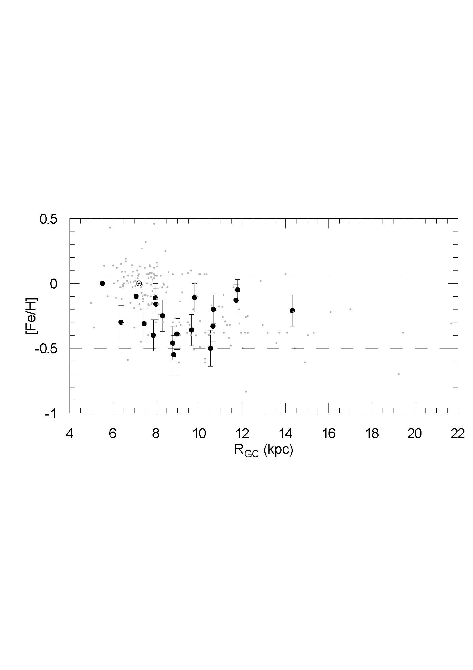
Figure 12: [Fe/H] versus $R_{GC}$ for the 20 O​Cs. Filled and grey dots represent the values of this work and the Dias catalogue, respectively. Horizontal lines denote the range of $[Fe/H]=[+0.05,~{}-0.50]$ of Friel et al. (2002). At $([Fe/H],~{}R_{\odot})=[0,~{}8.3]$ the big circle shows the solar position.

7 Metal-abundance gradient and Age-Metallicity Relation

By assuming $R_{\odot}=8.3\pm 0.23$ kpc, given by Brunthaler et al. (2011), the Galactocentric distances of 20 O​Cs have been calculated from the heliocentric distances, d, in Column 9 of Table 6. The plot of [Fe/H] versus R_GC (kpc) for the 20 O​Cs is given in Fig. 12, where filled dots show [Fe/H] and R_GC for this sample, while grey dots represent the values of 178 O​Cs in the Dias catalogue for which metal-abundance determinations are available, but which represent a more inhomogeneous sample with probable systematic differences. The Sun is located at $([Fe/H],~{}R_{\odot})=[0,~{}8.3]$. However, our sample is rather small and may contain selection biases. Moreover, our sample includes only a few clusters in each of the quadrants I, II, III of the Galactic disc, and metal-poor old O​Cs, are not well represented. These kinds of biases may lead to possible misinterpretations for mean [Fe/H], R_GC, and age-metallicity relations. However, the 20 O​Cs, in our sample do have the advantage of being uniformly analysed, and homogeneous regarding the instrumentation, observing techniques, reduction methods, and photometric calibrations.

In Fig. 12 horizontal lines denote the limits of [Fe/H]$=[+0.05,-0.50]$ suggested by Friel et al. (2002) for the Galactic O​Cs. However, recent spectroscopic studies of O​Cs indicate that there are, at least, more metal-poor O​Cs as compared to these limits. For example, Yong et al. (2005) have measured the spectroscopic abundance of Be 31 as $[Fe/H]=-0.57\pm 0.23$, which is somewhat more metal-poor. The metal abundances of 178 O​Cs in Dias catalogue fall in the range $-0.84\leq[Fe/H]\leq+0.46$, and NGC 436 in our sample is the most metal-poor cluster with [Fe/H]$=-0.55\pm 0.33$ dex, while Be 37 the most metal-rich with [Fe/H]$=-0.05\pm 0.08$ dex.

When a fit is applied for the 20 O​Cs, in the range of $6.82\leq R_{GC}\leq 15.37$ kpc in Fig. 12, a global abundance gradient of $+0.002\pm 0.022$ dex/kpc is calculated indicating that there is no correlation between [Fe/H] and R_GC (kpc) over this wide range. However, the works of Twarog et al. (1997), Magrini et al. (2009), Lepine et al. (2011), and Scarano & Lepine (2013) have shown that abundance gradients correlating [Fe/H] with R_GC for O​Cs should take into account a possible discontinuity at $R_{GC}\approx 8$–$10$ kpc.

Figure 13 shows an age-metallicity plot from the corresponding values of our 20 O​Cs plus those from Dias catalogue. It is clear from Fig. 13 that there is not any significant correlation between the ages and metal abundances for the 20 O​Cs. However, it is quite difficult to draw any firm conclusions due to the small sample and to the deficiency of old O​Cs in the present sample, but the Dias sample of Fig. 13 also shows little correlation. Carraro et al. (1998), Chen et al. (2003), and Salaris et al. (2004) also did not find any relation between the ages and metallicities for their O​Cs. The significant scatter in the ages and metallicities dominates and hides any possible small correlation. The reason for this scatter is due to orbital diffusion, radial mixing, and radial migration (Schönrich & Binney, 2009), as well as inhomogeneous chemical evolution in the Galactic disc (Haywood, 2008).

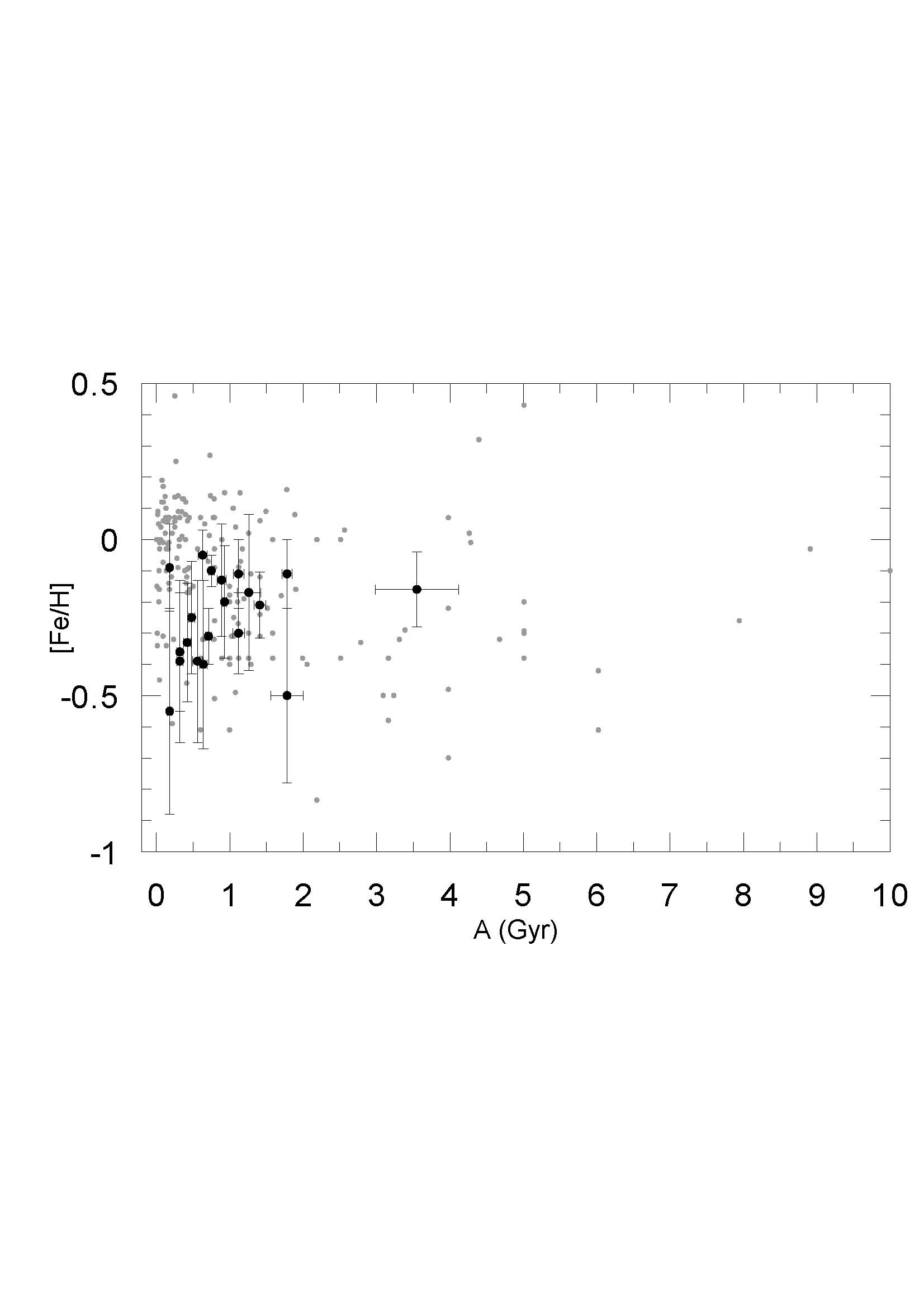
Figure 13: [Fe/H] versus A (Gyr) for the 20 O​Cs (filled dots). The grey dots represent the values in the Dias catalogue.

8 Spatial distribution of 20 O​Cs

Fig. 14 shows the spatial distribution of the 20 O​Cs (filled-circles and open-diamond symbols) in terms of the Galactic longitude with five spiral arms overlaid. This schematic projection of the Galaxy is seen from the north pole. As is evident from Fig. 14, the number of old O​Cs is low in the Galactic center direction. To first order this is probably due to our small sample plus our selection procedure, and the interstellar extinction, which is very strong mainly in these directions. But also, this is partly due to the high frequency of encounters with Giant Molecular Clouds (GMCs) inside the Solar circle, as discussed by Gieles et al. (2006) and Camargo et al. (2009), which tends to reduce the relative number of O​Cs.

Figure 14: The spatial distribution of the 20 O​Cs with five spiral arms overlaid and in terms of Galactic longitude. This schematic projection of the Galaxy is seen from the North Galactic Pole. Filled circles and open diamonds show the clusters with $[Fe/H]\geq-0.25$ and $[Fe/H]<-0.25$, respectively. The cluster names, metallicities, Galactocentric distances, and ages are listed below the figure for their respective quadrants.

Fig. 14 represents an (X, Y) projection in terms of both the metallicity and the Galactic longitude. Filled circles and open diamonds show the O​Cs with $[Fe/H]\geq-0.25$ and $[Fe/H]<-0.25$, respectively. Metal abundances, Galactocentric distances, and ages of these O​Cs of Fig. 14 are also presented in terms of the Galactic quadrant. There is not any indication that the distribution of the metal abundance of the O​Cs is a function of the quadrant in the (X, Y) plane of Fig. 14. Young clusters, $A<1$ Gyr, with $[Fe/H]<-0.30$ are mostly located in the Galactic anticentre directions, except for NGC 7062, which is located on the border of quadrants I and II.

A $|z|$ versus $R_{GC}$ plot is displayed in Fig. 15. Diamonds and filled circles show $A\leq 0.5$ Gyr and $A>0.5$ Gyr, respectively. The sun is located at $(R_{GC},z)=(8.3,~{}0.0148)$ kpc; the $z$ distance of the Sun has been taken from Chen et al. (1999). The O​Cs in Fig. 15 are mostly distributed at the distances, $|z|<0.3$ kpc and $R_{GC}<10$ kpc. However, for six O​Cs with $R_{GC}>10$ kpc, three reach vertical Galactic distances $|z|>0.5$ kpc. These O​Cs are located in the Galactic anticentre direction, $160^{\circ}<$ l $<228^{\circ}$, as is evident from Fig. 14 and Table 6.

The presence of this kind of cluster, moderately young and metal-poor, may have originated from the Galactic anticentre over-densities, such as that of Canis Major (Martin et al., 2004; Bellazzini et al., 2004) and of the Monoceros ring (Newberg et al., 2002). Having inspected the Galactic coordinates of these O​Cs, given in Table 6, it appears that they may not be associated with the Canis Major dwarf galaxy ($\it{l},~{}\it{b}$)=($240^{\circ}$,$-8^{\circ}$). However, since these accreting dwarf galaxies have long tidal tails both preceding and following them, a good agreement of the coordinates is not an exact test.

Similar to this paper, Yong et al. (2005, 2012) find from their O​Cs that the disc metallicity gradient becomes flat beyond $R_{GC}=10$–$12$ kpc, and they discuss the possibility that these O​Cs may be associated with an accreted dwarf galaxy, or may have formed as a result of star formation triggered by merger events in the outer disc. On the other hand, from observational photometric evidence for a group of young B5–A0 stars along the line of sight to the Canis Major over-density and also the presence of an older metal-poor population probably belonging to the Galactic thick disc or halo, Carraro et al. (2008) interpret these O​Cs as due to the effects of the structure of the Local and Outer spiral arms as well as the distortion produced by the Galactic warp.

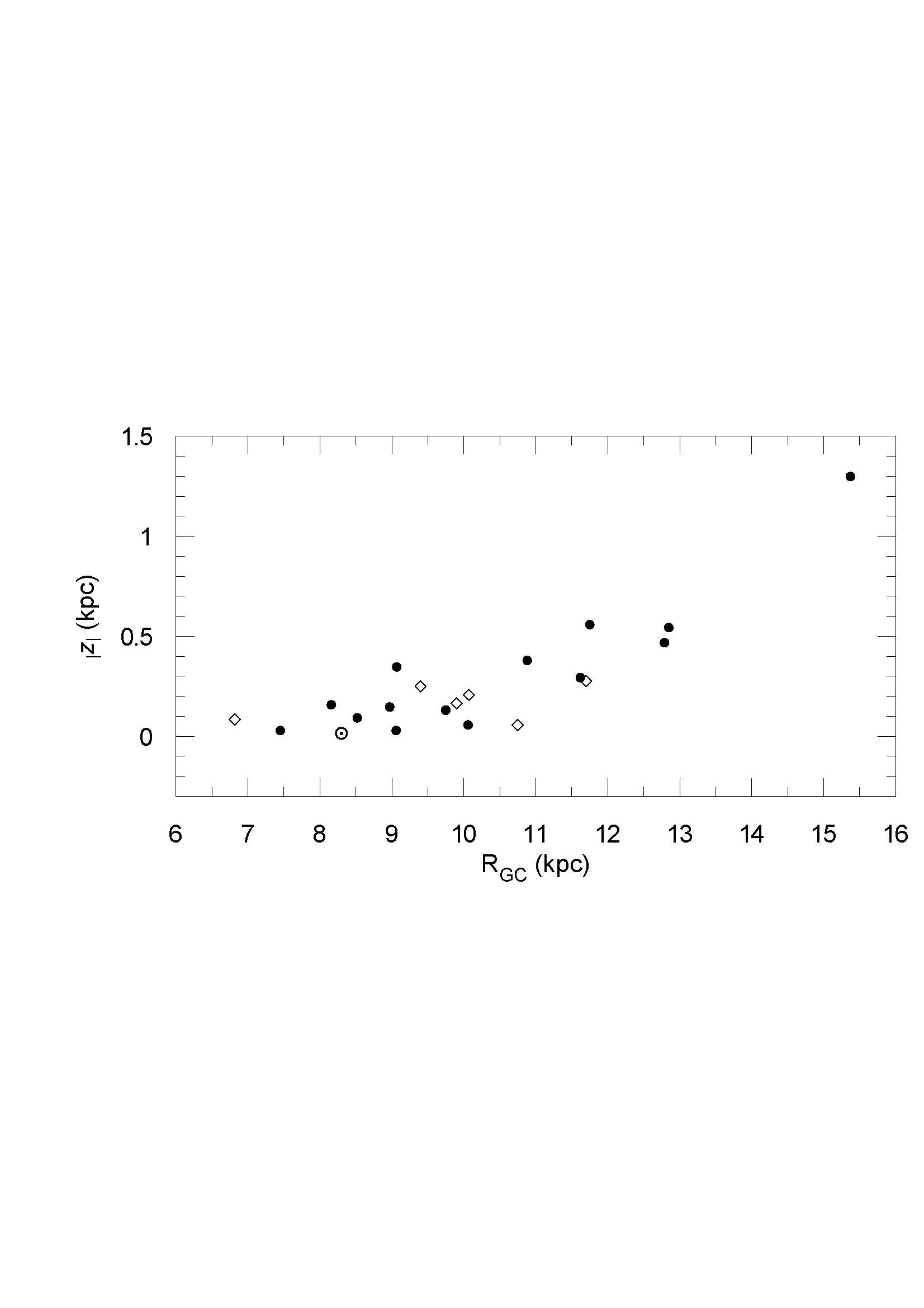
Figure 15: $|z|$ versus $R_{GC}$ for the 20 O​Cs. Diamonds and filled circles show $A\leq 0.5$ Gyr and $A>0.5$ Gyr, respectively. The Sun is located at $(R_{GC},z)=(8.3,0.0148)$ kpc.

9 RC and BS candidates

Ten possible RC groups have been identified in the CM diagrams for the following O​Cs: NGC 6802, NGC 7062, Ki 05, NGC 1798, NGC 7142, Be 35, Be 37, Ki 23, NGC 2304, and NGC 2360, with single RC stars probable in NGC 6866 and Ru 01. High mass stars (and their evolved products, RC/RG stars) are transferred to the cores of the O​Cs as a consequence of mass segregation. The SAFE algorithm is capable of emphasizing this kind of star by focusing on the central parts of the 20 O​Cs, which are small or comparable to the size of the CCD within the SPMO survey. One can expect to detect these possible RC stars in these O​Cs due to their intermediate ages (Table 6). The other O​Cs are younger, so it is reasonable not to detect RC candidates. Surprisingly, no obvious RC stars have been identified in Be 73 with an intermediate age of $A=1.41$ Gyr.

The possible RC candidates have been listed in Table S5 in the supplementary section. RC stars are useful as standard candles for estimating the distances to these O​Cs, or conversely their distances can be utilised as an initial test of their membership in a given cluster once its distance has been determined by main-sequence fitting in a CM diagram. The mean absolute magnitudes of $\langle M_{\rm V}\rangle=+0.60\pm 0.10$ (Twarog et al., 1997) and $\langle M_{\rm I}\rangle=-0.22\pm 0.03$ (Groenewegen, 2008) allow us to assign mean distances and their errors for RC candidates from their observed magnitudes, using the relations of $d=10^{(V-M_{V}+5-A_{\rm V})/5}$ and $\sigma_{\rm d}$ = $1\over 5$d$\times\ln(10)\times\sqrt{\sigma_{\rm V}^{2}+\sigma_{M_{\rm V}}^{2}+\sigma_{A_{\rm V}}^{2}}$ for the visual magnitude, with similar equations for $I$. Here, the total absorption relations of ${A_{\rm V}}=3.1~{}E(B$–$V)$ and $A_{\rm I}=1.98~{}E(B$–$V)$ (Gim et al., 1998), are used, with the $E(B$–$V)$ values given in Table 6 of this paper. The magnitudes of $I$ and $V$ in Columns 3–4 of Table S5 are used for estimating the $d_{\rm I}$ and $d_{\rm V}$ distances (in kpc) of these RC candidates, which are listed in Columns 5–6 of this same table, while the $(\alpha,~{}\delta)$ coordinates are listed in Columns 1–2.

The distances in Table S5 for each RC candidate have been compared to the distances from the $V,(B$–$V)$ and $V,(V$–$I)$ CM diagrams, which are also presented in Table S5 in the header for each cluster together with its name. Those stars which show combined 1-$\sigma$ agreement within the uncertainties of these two distances in Table S5 have been assigned as members (M), otherwise as non-members (NM), as shown at the end of Columns 5 and 6. However, this membership test has been done considering only distance criteria. For the confirmation of their cluster memberships, spectroscopic (radial velocity) observations and proper motion data are needed for these RC candidates, as well as for other members of these O​Cs.

From close inspection of the CC and CM diagrams of the 20 O​Cs, 12 B​S candidates with $V{\lesssim}15.60$ $(V_{0}{\lesssim}14.50)$ and $(B$–$V){\lesssim}0.80$ $((B$–$V)_{0}{\lesssim}0.45)$ in the CM diagram of NGC 7142 have been classified (see Fig. S8 in the supplementary section, where these B​S candidates have been marked with open squares). These limits for $V_{0}$ and $(B$–$V)_{0}$, which B​Ss occupy in CM diagrams, are similar to those given by Carney (2001, fig. 19) and Carraro et al. (2010b, fig. 10). However, the early-type, bluer, and brighter B​S candidates with $0.05\leq(B$–$V)_{0}\leq 0.41$ in the CM diagram of NGC 7142 may also be field stars between us and the cluster, as noticed by Carraro et al. (2010b). These are the three additional stars in the CM diagram of NGC 7142, in the same region as the BS candidates, but which are not marked as such. The coordinates $(\alpha,~{}\delta)$ and $BV\!RI$ photometry of these candidates are given in Table S6 (see the supplementary section).

10 Conclusions

Our main conclusions are as follows:

1. Twenty O​Cs, observed with the 84 cm telescope at SPMO, provide the advantage of having been uniformly and homogeneously processed regarding instrumentation, observing techniques, reduction methods, and analyses. The fundamental astrophysical parameters of these 20 O​Cs: interstellar reddenings, $E(B$–$V)$; photometric metallicities and mass-fraction heavy-element abundances ([Fe/H], Z); distance moduli, $(V_{0}$–$M_{\rm V})$, and distances, $d$ (kpc); plus ages, $A$ (Gyr), have been derived, and should be internally quite precise.

2. Differences in interstellar reddenings, metallicities, distance moduli, and ages, as compared to the literature, have been studied. Systematic differences, when found, are mainly due to the usage of distinct mean-colour relations versus isochrones, which correspond to differing element abundances, internal stellar physics, and colour-temperature relations. Different interstellar reddenings, as well as different assumptions, or measurements, for the stellar metallicities contribute greatly to these kinds of systematic offsets for the distances and ages.

3. The correlation coefficient of 0.86 indicates that the morphological ages, which are derived from the morphological indices $\delta V$ and $\delta 1$ in the CM diagrams, are fairly consistent with the isochrone ages of 12 O​Cs, for the ones with the presence of good RC and RG candidates. For four O​Cs, Ki 05, NGC 7142, Be 35, and NGC 2304, the differences of $\Delta logA$ are quite small, at the level of $\pm 0.01$ dex, as is seen in Fig. 11(b). For the other eight O​Cs, age differences fall in the range $\Delta logA=[-0.18,~{}+0.19]$.

4. For our sample of 20 O​Cs, their interstellar reddenings extend over $0.01\pm 0.07\leq E(B$–$V)\leq 0.80\pm 0.07$ [NGC 2360; NGC 6802]; their distances over $0.83\pm 0.01\leq d\leq 7.93\pm 0.11$ kpc [NGC 2215; Be 73]; and their ages over $0.18\pm 0.01\leq A\leq 3.55\pm 0.57$ Gyr [NGC 6694; NGC 7142]. (See Table 6.) All 20 O​Cs fall in Galactic quadrants I, II, and III, and 15 fall close to the anticentre direction, $125^{\circ}$ $<$ $l$ $<$ $235^{\circ}$.

5. For these 20 O​Cs, which have $6.82\leq R_{GC}\leq 15.37$ kpc, there is no correlation between [Fe/H] and $R_{GC}$ over this wide extent (Fig. 12). Our 20 O​Cs range over $-0.55\pm 0.33\leq[Fe/H]\leq-0.05\pm 0.08$ dex [NGC 436; Be 37].

6. Also, there is not any correlation between the cluster ages and metal abundances for these 20 O​Cs despite a 0.50 dex range in [Fe/H], as shown in Fig. 13. As discussed in the literature, this is caused by inhomogeneous chemical enhancements in the Galactic disc (Haywood, 2008; Jacobson et al., 2011), orbital diffusion, and radial migration and mixing of O​Cs (Schönrich & Binney, 2009). These O​Cs have probably originated from differing Galactic radii and/or from various star forming regions (Lepine et al., 2011).

7. The presence of young, metal-poor O​Cs in the second and third Galactic quadrants (Fig. 14) suggests that they may have originated from the Galactic anticentre over-densities, such as that in Canis Major (Martin et al., 2004; Bellazzini et al., 2004) or in the Monoceros ring (Newberg et al., 2002), as discussed by (Carraro et al., 2010a). Six of such O​Cs from our sample are located in the outer Galactic disc, R_GC $>$ 8.3 kpc (Fig. 14)). According to Yong et al. (2005), these O​Cs may be associated with an accreted dwarf galaxy or may have formed as a result of star formation triggered by merger events in the outer disc.

8. In addition, Fig. 15 shows that of the six O​Cs with R_GC $>$ 11 kpc, three have $|z|>0.5$ kpc, and all have $|z|\gtrsim 0.3$ kpc. As discussed by Carraro et al. (2008), their positions may be distorted by the Galactic warp and the existence of the local arms, the Perseus or Outer-arm. Momany et al. (2006) stress that the Canis Major properties point to an over-density reflecting a normal warped disc population rather than an accreted dwarf galaxy. These O​Cs have mostly intermediate ages, A $>$ 0.5 Gyr, supporting such an interpretation, i.e. a natural consequence of the Galactic disc’s warp rather than an accretion event.

9. Some RC and BS candidates are given in Tables S5 and S6, respectively, having been classified from the CM diagram for a subset of the 20 O​Cs; 12 O​Cs show RC candidates, and NGC 7142, BS candidates. These are proposed for future radial-velocity and proper-motion observations to confirm their membership in these O​Cs.

11 Supplementary Materials

Fundamental astrophysical parameters, plus CC and CM diagrams, for 19 O​Cs. The tables of fundamental astrophysical parameters for 19 O​Cs have been given in Tables S1–S4, and the CC and CM diagrams as Figs. S1–S19. “log($A$)-interval” in the tables refers to the derived range in ages possible from the isochrone pairs plotted in Figs. S1–S19. Possible RC candidates, which are classified in the CM diagrams of 12 O​Cs, are listed in Table S5. The data for possible BS candidates in NGC 7142 have been presented in Table S6.

Table S1: The derived astrophysical parameters of the O​Cs, NGC 6694, NGC 6802, NGC 6866, NGC 7062, and NGC 436.

Colour	$(V_{0}$–$M_{V})$	$d$ (kpc)	log($A$)-interval	log($A$)	$A$ (Gyr)
NGC6694: $E(B$–$V)=0.51\pm 0.06$,    $[Fe/H]=-0.09\pm 0.14$,    $Z=0.016\pm 0.005$
$(B$–$V)$	11.10$\pm$0.08	1.66$\pm$0.06	-	8.25$\pm$0.05	0.18$\pm$0.02
$(R$–$I)$	11.10$\pm$0.10	1.66$\pm$0.08	-	8.25$\pm$0.05	0.18$\pm$0.02
$(V$–$I)$	11.10$\pm$0.10	1.66$\pm$0.08	-	8.25$\pm$0.05	0.18$\pm$0.02
$(V$–$R)$	11.10$\pm$0.10	1.66$\pm$0.08	-	8.25$\pm$0.05	0.18$\pm$0.02
$(B$–$R)$	11.10$\pm$0.10	1.66$\pm$0.08	-	8.25$\pm$0.05	0.18$\pm$0.02
Mean	11.10$\pm$0.04	1.66$\pm$0.03		8.25$\pm$0.02	0.18$\pm$0.01
NGC 6802: $E(B$–$V)=0.80\pm 0.07$,    $[Fe/H]=-0.30\pm 0.13$,    $Z=0.009\pm 0.003$
$(B$–$V)$	11.20$\pm$0.10	1.74$\pm$0.08	9.00$-$9.05	9.05$\pm$0.05	1.12$\pm$0.14
$(R$–$I)$	11.10$\pm$0.15	1.66$\pm$0.12	9.00$-$9.05	9.05$\pm$0.10	1.12$\pm$0.29
$(V$–$I)$	11.20$\pm$0.15	1.74$\pm$0.12	9.00$-$9.05	9.05$\pm$0.10	1.12$\pm$0.29
$(V$–$R)$	11.20$\pm$0.10	1.74$\pm$0.08	9.00$-$9.05	9.05$\pm$0.10	1.12$\pm$0.29
$(B$–$R)$	11.20$\pm$0.10	1.74$\pm$0.08	9.00$-$9.05	9.05$\pm$0.05	1.12$\pm$0.14
Mean	11.19$\pm$0.05	1.73$\pm$0.04		9.05$\pm$0.03	1.12$\pm$0.08
NGC6866: $E(B$–$V)=0.06\pm 0.05$,    $[Fe/H]=-0.10\pm 0.05$,    $Z=0.015\pm 0.002$
$(B$–$V)$	10.70$\pm$0.02	1.38$\pm$0.01	8.75$-$8.85	8.85$\pm$0.05	0.71$\pm$0.09
$(R$–$I)$	10.50$\pm$0.05	1.26$\pm$0.03	8.80$-$8.90	8.90$\pm$0.05	0.79$\pm$0.10
$(V$–$I)$	10.50$\pm$0.08	1.26$\pm$0.05	8.80$-$8.90	8.90$\pm$0.05	0.79$\pm$0.10
$(V$–$R)$	10.50$\pm$0.06	1.26$\pm$0.04	8.80$-$8.90	8.90$\pm$0.05	0.79$\pm$0.10
$(B$–$R)$	10.50$\pm$0.03	1.26$\pm$0.02	8.80$-$8.90	8.90$\pm$0.05	0.79$\pm$0.10
Mean	10.61$\pm$0.02	1.32$\pm$0.01		8.89$\pm$0.02	0.75$\pm$0.04
NGC 7062: $E(B$–$V)=0.43\pm 0.08$,    $[Fe/H]=-0.31\pm 0.09$,    $Z=0.010\pm 0.002$
$(B$–$V)$	11.40$\pm$0.01	1.91$\pm$0.12	8.75$-$8.85	8.85$\pm$0.05	0.71$\pm$0.09
$(R$–$I)$	11.40$\pm$0.07	1.91$\pm$0.06	8.75$-$8.85	8.85$\pm$0.05	0.71$\pm$0.09
$(V$–$I)$	11.40$\pm$0.06	1.91$\pm$0.05	8.75$-$8.85	8.85$\pm$0.05	0.71$\pm$0.09
$(V$–$R)$	11.40$\pm$0.03	1.91$\pm$0.03	8.75$-$8.85	8.85$\pm$0.05	0.71$\pm$0.09
$(B$–$R)$	11.40$\pm$0.03	1.91$\pm$0.04	8.75$-$8.85	8.85$\pm$0.05	0.71$\pm$0.09
Mean	11.40$\pm$0.02	1.91$\pm$0.02		8.84$\pm$0.02	0.71$\pm$0.04
NGC 436: $E(B$–$V)=0.40\pm 0.07$,    $[Fe/H]=-0.55\pm 0.33$,    $Z=0.005\pm 0.004$
$(B$–$V)$	11.90$\pm$0.09	2.40$\pm$0.10	-	8.25$\pm$0.20	0.18$\pm$0.10
$(R$–$I)$	11.90$\pm$0.20	2.40$\pm$0.22	-	8.25$\pm$0.20	0.18$\pm$0.10
$(V$–$I)$	11.90$\pm$0.10	2.40$\pm$0.11	-	8.25$\pm$0.10	0.18$\pm$0.05
$(V$–$R)$	11.90$\pm$0.10	2.40$\pm$0.11	-	8.25$\pm$0.15	0.18$\pm$0.07
$(B$–$R)$	11.90$\pm$0.10	2.40$\pm$0.11	-	8.30$\pm$0.20	0.20$\pm$0.12
Mean	11.90$\pm$0.05	2.40$\pm$0.05		8.26$\pm$0.07	0.18$\pm$0.03

Table S2: The derived astrophysical parameters of the O​Cs, NGC 1798, NGC 1857, NGC 7142, Be 73, and Haf 04.

Colour	$(V_{0}$–$M_{V})$	$d$ (kpc)	log($A$)-interval	log($A$)	$A$ (Gyr)
NGC 1798: $E(B$–$V)=0.47\pm 0.07$,    $[Fe/H]=-0.50\pm 0.28$,    $Z=0.006\pm 0.004$
$(B$–$V)$	12.70$\pm$0.07	3.47$\pm$0.12	9.15$-$9.25	9.25$\pm$0.05	1.78$\pm$0.22
$(R$–$I)$	12.70$\pm$0.15	3.47$\pm$0.24	9.15$-$9.25	9.25$\pm$0.10	1.78$\pm$0.46
$(V$–$I)$	12.70$\pm$0.15	3.47$\pm$0.24	9.15$-$9.25	9.25$\pm$0.10	1.78$\pm$0.46
$(V$–$R)$	12.70$\pm$0.05	3.47$\pm$0.08	9.15$-$9.25	9.25$\pm$0.05	1.78$\pm$0.22
$(B$–$R)$	12.70$\pm$0.10	3.47$\pm$0.16	9.15$-$9.25	9.25$\pm$0.05	1.78$\pm$0.22
Mean	12.70$\pm$0.04	3.47$\pm$0.06		9.25$\pm$0.03	1.78$\pm$0.22
NGC 1857: $E(B$–$V)=0.47\pm 0.08$,    $[Fe/H]=-0.36\pm 0.19$,    $Z=0.008\pm 0.003$
$(B$–$V)$	12.00$\pm$0.07	2.51$\pm$0.08	8.40$-$8.50	8.50$\pm$0.10	0.32$\pm$0.08
$(R$–$I)$	12.00$\pm$0.20	2.51$\pm$0.23	8.40$-$8.50	8.50$\pm$0.15	0.32$\pm$0.13
$(V$–$I)$	12.00$\pm$0.10	2.51$\pm$0.12	8.40$-$8.50	8.50$\pm$0.10	0.32$\pm$0.08
$(V$–$R)$	12.00$\pm$0.10	2.51$\pm$0.12	8.40$-$8.50	8.50$\pm$0.10	0.32$\pm$0.08
$(B$–$R)$	11.90$\pm$0.10	2.40$\pm$0.11	8.45$-$8.55	8.55$\pm$0.10	0.35$\pm$0.09
Mean	11.98$\pm$0.04	2.49$\pm$0.05		8.51$\pm$0.05	0.32$\pm$0.04
NGC 7142: $E(B$–$V)=0.35\pm 0.08$,    $[Fe/H]=-0.16\pm 0.12$,    $Z=0.013\pm 0.004$
$(B$–$V)$	11.60$\pm$0.11	2.10$\pm$0.11	9.45$-$9.55	9.55$\pm$0.15	3.55$\pm$1.46
$(R$–$I)$	11.60$\pm$0.20	2.10$\pm$0.19	9.45$-$9.55	9.55$\pm$0.15	3.55$\pm$1.46
$(V$–$I)$	11.60$\pm$0.10	2.10$\pm$0.10	9.45$-$9.55	9.55$\pm$0.15	3.55$\pm$1.46
$(V$–$R)$	11.60$\pm$0.10	2.10$\pm$0.10	9.45$-$9.55	9.55$\pm$0.15	3.55$\pm$1.46
$(B$–$R)$	11.60$\pm$0.10	2.10$\pm$0.10	9.45$-$9.55	9.55$\pm$0.10	3.55$\pm$0.92
Mean	11.60$\pm$0.05	2.10$\pm$0.05		9.55$\pm$0.06	3.55$\pm$0.57
Be 73: $E(B$–$V)=0.28\pm 0.06$,    $[Fe/H]=-0.21\pm 0.06$,    $Z=0.012\pm 0.002$
$(B$–$V)$	14.50$\pm$0.04	7.94$\pm$0.15	9.10$-$9.15	9.15$\pm$0.05	1.41$\pm$0.17
$(R$–$I)$	14.45$\pm$0.10	7.76$\pm$0.36	9.10$-$9.15	9.15$\pm$0.10	1.41$\pm$0.37
$(V$–$I)$	14.50$\pm$0.10	7.94$\pm$0.37	9.10$-$9.15	9.15$\pm$0.05	1.41$\pm$0.17
$(V$–$R)$	14.50$\pm$0.10	7.94$\pm$0.37	9.10$-$9.15	9.15$\pm$0.05	1.41$\pm$0.17
$(B$–$R)$	14.50$\pm$0.05	7.94$\pm$0.18	9.10$-$9.15	9.15$\pm$0.05	1.41$\pm$0.17
Mean	14.50$\pm$0.03	7.93$\pm$0.11		9.15$\pm$0.02	1.41$\pm$0.08
Haf04: $E(B$–$V)=0.47\pm 0.09$,    $[Fe/H]=-0.33\pm 0.19$,    $Z=0.009\pm 0.008$
$(B$–$V)$	13.30$\pm$0.09	4.57$\pm$0.19	8.60$-$8.70	8.60$\pm$0.10	0.40$\pm$0.10
$(R$–$I)$	13.10$\pm$0.15	4.17$\pm$0.29	8.65$-$8.75	8.65$\pm$0.10	0.45$\pm$0.12
$(V$–$I)$	13.10$\pm$0.10	4.17$\pm$0.29	8.65$-$8.75	8.65$\pm$0.10	0.45$\pm$0.12
$(V$–$R)$	13.20$\pm$0.10	4.37$\pm$0.20	8.60$-$8.70	8.60$\pm$0.10	0.40$\pm$0.10
$(B$–$R)$	13.30$\pm$0.05	4.57$\pm$0.21	8.65$-$8.75	8.65$\pm$0.10	0.45$\pm$0.12
Mean	13.22$\pm$0.05	4.39$\pm$0.10		8.63$\pm$0.04	0.42$\pm$0.05

Table S3: The derived astrophysical parameters of the O​Cs, NGC 2215, Rup 01, Be 35, Be 37, and Haf 08.

Colour	$(V_{0}$–$M_{V})$	$d$ (kpc)	log($A$)-interval	log($A$)	$A$ (Gyr)
NGC 2215: $E(B$–$V)=0.23\pm 0.07$,    $[Fe/H]=-0.40\pm 0.27$,    $Z=0.008\pm 0.005$
$(B$–$V)$	9.60$\pm$0.07	0.83$\pm$0.03	8.80$-$8.85	8.80$\pm$0.05	0.63$\pm$0.08
$(R$–$I)$	9.60$\pm$0.10	0.83$\pm$0.04	8.85$-$8.90	8.85$\pm$0.10	0.71$\pm$0.18
$(V$–$I)$	9.60$\pm$0.10	0.83$\pm$0.04	8.85$-$8.90	8.85$\pm$0.10	0.71$\pm$0.18
$(V$–$R)$	9.60$\pm$0.05	0.83$\pm$0.02	8.80$-$8.85	8.80$\pm$0.05	0.63$\pm$0.08
$(B$–$R)$	9.60$\pm$0.05	0.83$\pm$0.02	8.80$-$8.85	8.80$\pm$0.10	0.63$\pm$0.16
Mean	9.60$\pm$0.03	0.83$\pm$0.01		8.81$\pm$0.03	0.64$\pm$0.05
Rup 01: $E(B$–$V)=0.17\pm 0.06$,    $[Fe/H]=-0.25\pm 0.18$,    $Z=0.011\pm 0.005$
$(B$–$V)$	10.90$\pm$0.05	1.51$\pm$0.04	8.65$-$8.70	8.65$\pm$0.05	0.45$\pm$0.05
$(R$–$I)$	10.80$\pm$0.15	1.45$\pm$0.10	8.70$-$8.75	8.70$\pm$0.10	0.50$\pm$0.13
$(V$–$I)$	10.80$\pm$0.15	1.45$\pm$0.10	8.70$-$8.75	8.70$\pm$0.10	0.50$\pm$0.13
$(V$–$R)$	10.80$\pm$0.10	1.45$\pm$0.07	8.70$-$8.75	8.70$\pm$0.05	0.50$\pm$0.06
$(B$–$R)$	10.80$\pm$0.10	1.45$\pm$0.07	8.70$-$8.75	8.70$\pm$0.10	0.50$\pm$0.13
Mean	10.85$\pm$0.04	1.48$\pm$0.03		8.68$\pm$0.03	0.48$\pm$0.04
Be 35: $E(B$–$V)=0.11\pm 0.07$,    $[Fe/H]=-0.13\pm 0.18$,    $Z=0.014\pm 0.006$
$(B$–$V)$	13.50$\pm$0.07	5.01$\pm$0.15	8.85$-$8.95	8.95$\pm$0.10	0.89$\pm$0.23
$(R$–$I)$	13.50$\pm$0.15	5.01$\pm$0.35	8.85$-$8.95	8.95$\pm$0.15	0.89$\pm$0.37
$(V$–$I)$	13.50$\pm$0.10	5.01$\pm$0.23	8.85$-$8.95	8.95$\pm$0.10	0.89$\pm$0.23
$(V$–$R)$	13.50$\pm$0.10	5.01$\pm$0.23	8.85$-$8.95	8.95$\pm$0.05	0.89$\pm$0.11
$(B$–$R)$	13.50$\pm$0.10	5.01$\pm$0.23	8.85$-$8.95	8.95$\pm$0.05	0.89$\pm$0.11
Mean	13.50$\pm$0.04	5.01$\pm$0.10		8.95$\pm$0.03	0.89$\pm$0.06
Be 37: $E(B$–$V)=0.05\pm 0.05$,    $[Fe/H]=-0.05\pm 0.08$,    $Z=0.017\pm 0.003$
$(B$–$V)$	13.60$\pm$0.03	5.25$\pm$0.07	8.80$-$8.85	8.80$\pm$0.05	0.63$\pm$0.07
$(R$–$I)$	13.60$\pm$0.10	5.25$\pm$0.24	8.80$-$8.85	8.80$\pm$0.05	0.63$\pm$0.08
$(V$–$I)$	13.60$\pm$0.10	5.25$\pm$0.24	8.80$-$8.85	8.80$\pm$0.10	0.63$\pm$0.16
$(V$–$R)$	13.65$\pm$0.10	5.37$\pm$0.25	8.80$-$8.85	8.80$\pm$0.05	0.63$\pm$0.08
$(B$–$R)$	13.60$\pm$0.05	5.25$\pm$0.12	8.80$-$8.85	8.80$\pm$0.05	0.63$\pm$0.08
Mean	13.60$\pm$0.02	5.25$\pm$0.06		8.80$\pm$0.02	0.63$\pm$0.06
Haf 08: $E(B$–$V)=0.32\pm 0.07$,    $[Fe/H]=-0.39\pm 0.26$,    $Z=0.008\pm 0.005$
$(B$–$V)$	11.90$\pm$0.06	2.40$\pm$0.07	8.60$-$8.75	8.75$\pm$0.10	0.56$\pm$0.15
$(R$–$I)$	11.80$\pm$0.10	2.30$\pm$0.11	8.60$-$8.75	8.75$\pm$0.15	0.56$\pm$0.23
$(V$–$I)$	11.90$\pm$0.10	2.40$\pm$0.11	8.60$-$8.75	8.75$\pm$0.10	0.56$\pm$0.15
$(V$–$R)$	11.90$\pm$0.10	2.40$\pm$0.11	8.60$-$8.75	8.75$\pm$0.10	0.56$\pm$0.15
$(B$–$R)$	11.90$\pm$0.10	2.40$\pm$0.11	8.60$-$8.75	8.75$\pm$0.10	0.56$\pm$0.15
Mean	11.88$\pm$0.04	2.38$\pm$0.04		8.75$\pm$0.05	0.56$\pm$0.07

Table S4: The derived astrophysical parameters of the O​Cs, Ki 23, NGC 2186, NGC 2304, and NGC 2360.

Colour	$(V_{0}$–$M_{V})$	$d$ (kpc)	log($A$)-interval	log($A$)	$A$ (Gyr)
Ki 23: $E(B$–$V)=0.03\pm 0.02$,    $[Fe/H]=-0.11\pm 0.11$,    $Z=0.015\pm 0.004$
$(B$–$V)$	12.40$\pm$0.04	3.02$\pm$0.05	$-$	9.25$\pm$0.03	1.78$\pm$0.13
$(R$–$I)$	12.40$\pm$0.10	3.02$\pm$0.14	$-$	9.25$\pm$0.05	1.78$\pm$0.22
$(V$–$I)$	12.40$\pm$0.10	3.02$\pm$0.14	$-$	9.25$\pm$0.05	1.78$\pm$0.22
$(V$–$R)$	12.40$\pm$0.05	3.02$\pm$0.07	$-$	9.25$\pm$0.03	1.78$\pm$0.13
$(B$–$R)$	12.40$\pm$0.05	3.02$\pm$0.07	$-$	9.25$\pm$0.03	1.78$\pm$0.13
Mean	12.40$\pm$0.02	3.02$\pm$0.03	9.25$\pm$0.02	1.78 $\pm$0.07
NGC 2186: $E(B$–$V)=0.26\pm 0.07$,    $[Fe/H]=-0.39\pm 0.26$,    $Z=0.008\pm 0.005$
$(B$–$V)$	11.40$\pm$0.03	1.91$\pm$0.03	8.50$-$8.60	8.50$\pm$0.10	0.32$\pm$0.08
$(R$–$I)$	11.40$\pm$0.15	1.91$\pm$0.13	8.50$-$8.60	8.50$\pm$0.15	0.32$\pm$0.13
$(V$–$I)$	11.40$\pm$0.15	1.91$\pm$0.13	8.50$-$8.60	8.50$\pm$0.15	0.32$\pm$0.13
$(V$–$R)$	11.40$\pm$0.10	1.91$\pm$0.09	8.55$-$8.65	8.55$\pm$0.10	0.35$\pm$0.09
$(B$–$R)$	11.40$\pm$0.10	1.91$\pm$0.09	8.50$-$8.60	8.50$\pm$0.10	0.32$\pm$0.08
Mean	11.40$\pm$0.03	1.91$\pm$0.03		8.51$\pm$0.05	0.32$\pm$0.04
NGC 2304: $E(B$–$V)=0.03\pm 0.03$,    $[Fe/H]=-0.20\pm 0.18$,    $Z=0.012\pm 0.005$
$(B$–$V)$	12.80$\pm$0.02	3.63$\pm$0.03	8.90$-$8.95	8.95$\pm$0.03	0.89$\pm$0.06
$(R$–$I)$	12.70$\pm$0.10	3.47$\pm$0.16	8.95$-$9.00	9.00$\pm$0.05	1.00$\pm$0.12
$(V$–$I)$	12.70$\pm$0.05	3.47$\pm$0.08	8.95$-$9.00	9.00$\pm$0.03	1.00$\pm$0.07
$(V$–$R)$	12.80$\pm$0.10	3.63$\pm$0.17	8.90$-$8.95	8.95$\pm$0.05	0.89$\pm$0.11
$(B$–$R)$	12.80$\pm$0.05	3.63$\pm$0.08	8.90$-$8.95	8.95$\pm$0.03	0.89$\pm$0.06
Mean	12.79$\pm$0.02	3.61$\pm$0.03		8.97$\pm$0.02	0.93$\pm$0.03
NGC 2360: $E(B$–$V)=0.09\pm 0.06$,    $[Fe/H]=-0.11\pm 0.11$,    $Z=0.015\pm 0.004$
$(B$–$V)$	10.30$\pm$0.05	1.15$\pm$0.03	9.00$-$9.05	9.05$\pm$0.05	1.12$\pm$0.14
$(R$–$I)$	10.30$\pm$0.10	1.15$\pm$0.05	9.00$-$9.05	9.05$\pm$0.08	1.12$\pm$0.23
$(V$–$I)$	10.20$\pm$0.05	1.10$\pm$0.03	9.00$-$9.05	9.05$\pm$0.05	1.12$\pm$0.14
$(V$–$R)$	10.20$\pm$0.05	1.10$\pm$0.03	9.00$-$9.05	9.05$\pm$0.05	1.12$\pm$0.14
$(B$–$R)$	10.30$\pm$0.05	1.15$\pm$0.03	9.00$-$9.05	9.05$\pm$0.05	1.12$\pm$0.14
Mean	10.25$\pm$0.02	1.12$\pm$0.01		9.05$\pm$0.02	1.12$\pm$0.07

Table S5: Possible RC candidates, which are classified in the CM diagrams of 12 O​Cs from our sample. The $(\alpha,~{}\delta)$ coordinates, the $I$ and $V$ magnitudes, and the the distances, $d_{\rm I}$ and $d_{\rm V}$, (in kpc) from the RC calibrations, are listed in Columns 1–2, 3–4, and 5–6, respectively. The distances $d_{\rm I}$ and $d_{\rm V}$, derived from CM plots, have also been given for each cluster in its header together with its name. The symbols “M” and “NM”, of Columns 5–6, indicate possible members and non-members according to distance comparisons.

$\alpha(^{\circ})$	$\delta(^{\circ})$	$I$	$V$	$d_{\rm I}$	$d_{\rm V}$
NGC 6802	$d_{\rm I}=1.74\pm 0.12$	$d_{\rm V}=1.74\pm 0.08$
292.6643	20.2566	12.554$\pm$0.003	14.619$\pm$0.005	1.73$\pm$0.11, M	2.03$\pm$0.22, M
292.6472	20.2642	12.657$\pm$0.002	14.692$\pm$0.004	1.81$\pm$0.12, M	2.10$\pm$0.23, M
292.6505	20.2758	12.734$\pm$0.002	14.735$\pm$0.004	1.88$\pm$0.12, M	2.14$\pm$0.24, NM
292.6286	20.2743	12.704$\pm$0.002	14.774$\pm$0.004	1.85$\pm$0.12, M	2.18$\pm$0.24, NM
292.6619	20.2335	12.852$\pm$0.002	14.879$\pm$0.003	1.98$\pm$0.13, M	2.29$\pm$0.25, NM
292.6327	20.2461	12.851$\pm$0.002	14.967$\pm$0.003	1.98$\pm$0.13, M	2.39$\pm$0.26, NM
292.6354	20.2632	12.898$\pm$0.002	14.980$\pm$0.005	2.03$\pm$0.13, NM	2.40$\pm$0.26, NM
292.6738	20.2562	12.971$\pm$0.002	14.996$\pm$0.004	2.10$\pm$0.14, NM	2.42$\pm$0.27, NM
292.6019	20.2584	12.996$\pm$0.001	15.037$\pm$0.005	2.12$\pm$0.14, NM	2.46$\pm$0.27, NM
292.6936	20.2544	13.054$\pm$0.001	15.094$\pm$0.004	2.18$\pm$0.14, NM	2.53$\pm$0.28, NM
NGC 6866	$d_{\rm I}=1.26\pm 0.05$	$d_{\rm V}=1.38\pm 0.01$
300.9904	44.1077	10.667$\pm$0.003	11.706$\pm$0.003	1.42$\pm$0.09, NM	1.53$\pm$0.12, NM
300.9799	44.1401	10.580$\pm$0.001	11.625$\pm$0.002	1.37$\pm$0.09, M	1.47$\pm$0.12, M
NGC 7062	$d_{\rm I}=1.91\pm 0.05$	$d_{\rm V}=1.91\pm 0.12$
320.8357	46.3748	10.971$\pm$0.008	12.417$\pm$0.004	1.17$\pm$0.12, NM	1.25$\pm$0.14, NM
320.8369	46.3736	11.521$\pm$0.004	12.940$\pm$0.007	1.51$\pm$0.16, NM	1.59$\pm$0.18, NM
320.8638	46.3705	11.509$\pm$0.002	12.981$\pm$0.003	1.50$\pm$0.16, NM	1.62$\pm$0.18, M
320.9146	46.3702	11.574$\pm$0.001	13.095$\pm$0.002	1.54$\pm$0.16, NM	1.71$\pm$0.19, M
320.8914	46.3852	11.531$\pm$0.001	13.102$\pm$0.003	1.51$\pm$0.16, NM	1.71$\pm$0.19, M
Ki05	$d_{\rm I}=1.74\pm 0.08$	$d_{\rm V}=1.74\pm 0.09$
48.6470	52.7242	13.213$\pm$0.006	14.988$\pm$0.004	2.57$\pm$0.27, NM	2.78$\pm$0.31, NM
48.6601	52.6974	13.203$\pm$0.006	14.947$\pm$0.003	2.56$\pm$0.27, NM	2.73$\pm$0.31, NM
48.6924	52.6893	12.918$\pm$0.006	14.712$\pm$0.003	2.24$\pm$0.23, M	2.45$\pm$0.28, NM
48.5764	52.7114	12.810$\pm$0.007	14.609$\pm$0.005	2.13$\pm$0.22, M	2.33$\pm$0.26, M
48.6160	52.7113	12.717$\pm$0.006	14.541$\pm$0.002	2.04$\pm$0.21, M	2.26$\pm$0.26, M
48.6462	52.7332	12.601$\pm$0.006	14.385$\pm$0.002	1.94$\pm$0.20, M	2.10$\pm$0.24, M
48.7148	52.7269	12.467$\pm$0.007	14.210$\pm$0.003	1.82$\pm$0.19, M	1.94$\pm$0.22, M
48.6806	52.7040	12.401$\pm$0.005	14.197$\pm$0.003	1.77$\pm$0.18, M	1.93$\pm$0.22, M
NGC 1798	$d_{\rm I}=3.47\pm 0.24$	$d_{\rm V}=3.47\pm 0.12$
77.8858	47.6875	13.708$\pm$0.006	15.123$\pm$0.003	3.98$\pm$0.35, M	4.10$\pm$0.40, NM
77.8938	47.6883	13.808$\pm$0.005	15.242$\pm$0.003	4.16$\pm$0.36, NM	4.34$\pm$0.42, NM
77.9343	47.6977	13.899$\pm$0.008	15.299$\pm$0.003	4.34$\pm$0.38, NM	4.45$\pm$0.44, NM
77.9175	47.6885	13.873$\pm$0.007	15.330$\pm$0.003	4.29$\pm$0.38, NM	4.51$\pm$0.44, NM
77.9600	47.6997	13.995$\pm$0.006	15.397$\pm$0.003	4.54$\pm$0.40, NM	4.66$\pm$0.46, NM
77.9427	47.7011	14.099$\pm$0.006	15.490$\pm$0.003	4.76$\pm$0.42, NM	4.86$\pm$0.48, NM
77.8680	47.7047	14.066$\pm$0.005	15.497$\pm$0.004	4.69$\pm$0.41, NM	4.88$\pm$0.48, NM
77.8698	47.6774	14.086$\pm$0.008	15.525$\pm$0.004	4.73$\pm$0.41, NM	4.94$\pm$0.48, NM
77.9460	47.6833	14.136$\pm$0.006	15.542$\pm$0.004	4.84$\pm$0.42, NM	4.98$\pm$0.49, NM
77.9427	47.6869	14.190$\pm$0.007	15.614$\pm$0.004	4.96$\pm$0.43, NM	5.15$\pm$0.50, NM
77.8992	47.6949	14.153$\pm$0.008	15.624$\pm$0.004	4.88$\pm$0.43, NM	5.17$\pm$0.51, NM
77.9163	47.7094	14.268$\pm$0.006	15.644$\pm$0.003	5.15$\pm$0.45, NM	5.22$\pm$0.51, NM
77.9197	47.6774	14.291$\pm$0.006	15.707$\pm$0.004	5.20$\pm$0.45, NM	5.37$\pm$0.53, NM
77.9542	47.6659	14.302$\pm$0.008	15.721$\pm$0.004	5.23$\pm$0.46, NM	5.41$\pm$0.53, NM
77.8936	47.6955	14.315$\pm$0.007	15.754$\pm$0.006	5.26$\pm$0.46, NM	5.49$\pm$0.54, NM

$\alpha(^{\circ})$	$\delta(^{\circ})$	$I$	$V$	$d_{\rm I}$	$d_{\rm V}$
NGC 7142	$d_{\rm I}=2.10\pm 0.10$	$d_{\rm V}=2.10\pm 0.11$
326.1734	65.7971	12.840$\pm$0.003	14.251$\pm$0.003	2.97$\pm$0.31, NM	3.26$\pm$0.37, NM
326.3668	65.7518	12.722$\pm$0.003	14.236$\pm$0.003	2.82$\pm$0.30, NM	3.24$\pm$0.36, NM
326.3041	65.8276	12.747$\pm$0.003	14.185$\pm$0.003	2.85$\pm$0.30, NM	3.16$\pm$0.36, NM
326.1826	65.7785	12.616$\pm$0.000	14.135$\pm$0.003	2.67$\pm$0.28, NM	3.10$\pm$0.35, NM
326.3872	65.7920	12.382$\pm$0.003	13.829$\pm$0.003	2.50$\pm$0.25, NM	2.68$\pm$0.30, NM
326.3351	65.8086	12.233$\pm$0.002	13.763$\pm$0.003	2.25$\pm$0.23, M	2.60$\pm$0.30, NM
326.2400	65.8102	12.319$\pm$0.002	13.738$\pm$0.002	2.33$\pm$0.24, M	2.57$\pm$0.29, NM
326.2530	65.7657	12.023$\pm$0.002	13.4966$\pm$0.002	2.04$\pm$0.21, M	2.30$\pm$0.26, M
Ru 01	$d_{\rm I}=1.45\pm 0.10$	$d_{\rm V}=1.51\pm 0.04$
99.0931	-14.1485	10.842$\pm$0.002	12.055$\pm$0.002	1.40$\pm$0.11, M	1.53$\pm$0.14 M
Be 35	$d_{\rm I}=5.01\pm 0.23$	$d_{\rm V}=5.01\pm 0.15$
107.4635	2.7182	13.095$\pm$0.003	14.168$\pm$0.003	4.16$\pm$0.38, NM	4.42$\pm$0.45, M
107.4976	2.6956	13.295$\pm$0.003	14.359$\pm$0.003	4.56$\pm$0.42, M	4.83$\pm$0.49, M
107.4861	2.7698	13.455$\pm$0.003	14.501$\pm$0.003	4.91$\pm$0.45, M	5.15$\pm$0.52, M
107.4932	2.7685	13.564$\pm$0.003	14.599$\pm$0.004	5.17$\pm$0.47, M	5.39$\pm$0.55, M
107.4923	2.7378	13.612$\pm$0.000	14.652$\pm$0.004	5.28$\pm$0.48, M	5.52$\pm$0.56, M
107.4935	2.7336	13.796$\pm$0.003	14.832$\pm$0.004	5.75$\pm$0.52, M	6.00$\pm$0.61, NM
107.4684	2.7372	13.784$\pm$0.004	14.811$\pm$0.004	5.72$\pm$0.52, M	5.94$\pm$0.60, NM
107.4698	2.7234	13.831$\pm$0.005	14.816$\pm$0.008	5.84$\pm$0.53, NM	5.96$\pm$0.60, NM
107.4899	2.7355	13.974$\pm$0.004	15.001$\pm$0.004	6.24$\pm$0.57 NM	6.49$\pm$0.66, NM
Be 37	$d_{\rm I}=5.25\pm 0.24$	$d_{\rm V}=5.25\pm 0.07$
110.1164	-1.0266	13.360$\pm$0.003	14.396$\pm$0.003	4.97$\pm$0.33, M	5.35$\pm$0.42, NM
110.0793	-1.0450	13.250$\pm$0.002	14.251$\pm$0.003	4.72$\pm$0.31, NM	5.00$\pm$0.40, M
110.0558	-0.9965	13.286$\pm$0.002	14.260$\pm$0.003	4.80$\pm$0.32, M	5.02$\pm$0.40, M
110.0808	-0.9972	13.528$\pm$0.005	14.432$\pm$0.004	5.37$\pm$0.35, M	5.44$\pm$0.43, M
110.0442	-0.9862	13.333$\pm$0.009	14.243$\pm$0.004	4.91$\pm$0.32, M	4.98$\pm$0.39, M
110.0810	-1.0268	13.337$\pm$0.002	14.242$\pm$0.003	4.92$\pm$0.32, M	4.98$\pm$0.39, M
110.0678	-1.0113	13.154$\pm$0.003	14.017$\pm$0.004	4.52$\pm$0.30, M	4.49$\pm$0.36, NM
110.0768	-1.0240	12.940$\pm$0.002	13.850$\pm$0.002	4.10$\pm$0.27, NM	4.16$\pm$0.33, NM
Ki 23	$d_{\rm I}=3.02\pm 0.14$	$d_{\rm V}=3.02\pm 0.05$
110.444	-0.9787	12.585$\pm$0.002	13.598$\pm$0.002	3.54$\pm$0.10, NM	3.81$\pm$0.20, NM
110.4522	-0.9922	12.375$\pm$0.002	13.428$\pm$0.002	3.21$\pm$0.09, M	3.52$\pm$0.19, NM
110.4692	-0.9875	12.477$\pm$0.001	13.572$\pm$0.002	3.37$\pm$0.10, NM	3.77$\pm$0.20, NM
NGC 2304	$d_{\rm I}=3.47\pm 0.08$	$d_{\rm V}=3.63\pm 0.03$
		I	V	$d_{I}$	dV
103.8089	17.9764	12.136$\pm$0.002	13.190$\pm$0.002	2.88$\pm$0.12, NM	3.16$\pm$0.19, NM
103.8109	17.9954	12.758$\pm$0.002	13.678$\pm$0.003	3.83$\pm$0.16, NM	3.95$\pm$0.24, NM
103.8096	17.9854	13.053$\pm$0.002	14.008$\pm$0.003	4.39$\pm$0.18, NM	4.60$\pm$0.28, NM
103.7918	17.9802	13.144$\pm$0.002	14.125$\pm$0.003	4.58$\pm$0.19, NM	4.86$\pm$0.29, NM
NGC 2360	$d_{\rm I}=1.10\pm 0.03$	$d_{\rm V}=1.15\pm 0.03$
109.4799	-15.6987	10.462$\pm$0.007	11.506$\pm$0.002	1.26$\pm$0.10, NM	1.33$\pm$0.12, NM
109.3857	-15.6498	10.457$\pm$0.005	11.485$\pm$0.003	1.26$\pm$0.10, NM	1.32$\pm$0.12, NM
109.4300	-15.6185	10.078$\pm$0.005	11.204$\pm$0.003	1.06$\pm$0.08, M	1.16$\pm$0.10, M
109.4528	-15.5971	10.301$\pm$0.007	11.354$\pm$0.003	1.17$\pm$0.09, M	1.24$\pm$0.11, M
109.4140	-15.6100	10.256$\pm$0.006	11.279$\pm$0.003	1.15$\pm$0.09, M	1.20$\pm$0.11, M
109.4293	-15.6256	10.062$\pm$0.006	11.089$\pm$0.002	1.05$\pm$0.08, M	1.10$\pm$0.10, M
109.4529	-15.6614	9.972$\pm$0.006	11.038$\pm$0.003	1.00$\pm$0.08, M	1.08$\pm$0.10, M
109.3985	-15.6252	10.061$\pm$0.005	11.058$\pm$0.002	1.05$\pm$0.08, M	1.09$\pm$0.10, M
109.3961	-15.6432	9.720$\pm$0.006	10.797$\pm$0.003	0.90$\pm$0.07, NM	0.96$\pm$0.09, NM
109.4474	-15.6358	9.578$\pm$0.007	10.732$\pm$0.003	0.84$\pm$0.07, NM	0.94$\pm$0.08, NM

Table S6: Possible BS candidates in NGC 7142. The coordinates, $(\alpha,~{}\delta)$, of the candidates are given in Columns 1–2, while $V$ magnitudes and colour indices for $VBRI$ photometry, together with their uncertainties, have been listed in Columns 3–8.

$\alpha(^{\circ})$	$\delta(^{\circ})$	$V$	$B-V$	$R-I$	$V-I$	$V-R$	$B-R$
326.3132	65.8234	15.443$\pm$0.006	0.676$\pm$0.010	0.499$\pm$0.009	0.894$\pm$0.008	0.395$\pm$0.009	1.071$\pm$0.011
326.2488	65.7197	15.436$\pm$0.006	0.732$\pm$0.011	0.498$\pm$0.009	0.945$\pm$0.008	0.447$\pm$0.009	1.179$\pm$0.011
326.2103	65.8170	15.406$\pm$0.004	0.764$\pm$0.008	0.522$\pm$0.005	0.979$\pm$0.005	0.457$\pm$0.006	1.221$\pm$0.008
326.2602	65.7404	15.344$\pm$0.004	0.744$\pm$0.008	0.530$\pm$0.005	1.002$\pm$0.005	0.472$\pm$0.006	1.216$\pm$0.008
326.2210	65.7472	15.201$\pm$0.004	0.712$\pm$0.007	0.499$\pm$0.006	0.888$\pm$0.006	0.389$\pm$0.006	1.101$\pm$0.007
326.3679	65.8245	15.097$\pm$0.004	0.550$\pm$0.007	0.417$\pm$0.006	0.739$\pm$0.006	0.322$\pm$0.006	0.872$\pm$0.007
326.1821	65.7889	14.913$\pm$0.004	0.572$\pm$0.006	0.365$\pm$0.004	0.702$\pm$0.005	0.337$\pm$0.005	0.909$\pm$0.005
326.3591	65.7573	14.900$\pm$0.004	0.760$\pm$0.007	0.500$\pm$0.004	0.945$\pm$0.005	0.445$\pm$0.005	1.205$\pm$0.007
326.4176	65.7372	14.859$\pm$0.004	0.660$\pm$0.007	0.467$\pm$0.004	0.855$\pm$0.005	0.388$\pm$0.005	1.048$\pm$0.007
326.1879	65.8063	14.630$\pm$0.003	0.417$\pm$0.005	0.322$\pm$0.006	0.569$\pm$0.005	0.247$\pm$0.005	0.664$\pm$0.006
326.2186	65.7718	14.476$\pm$0.003	0.401$\pm$0.005	0.305$\pm$0.003	0.507$\pm$0.005	0.202$\pm$0.005	0.603$\pm$0.006
326.2166	65.7727	14.223$\pm$0.003	0.442$\pm$0.005	0.323$\pm$0.004	0.555$\pm$0.004	0.232$\pm$0.004	0.674$\pm$0.005

Figure S2: Panel (a): the $(U$–$B,B$–$V)$ diagram of NGC 6802. Panels (b)–(f): CM diagrams of $(V,B$–$V)$, $(V,R$–$I)$, $(V,V$–$I)$, $(V,V$–$R)$, and $(V,B$–$R)$. The symbols are the same as Fig. 1 and Figs. 2–3.

Figure S4: Panel (a): the $(U$–$B,B$–$V)$ diagram of NGC 7062. Panels (b)–(f): CM diagrams of $(V,B$–$V)$, $(V,R$–$I)$, $(V,V$–$I)$, $(V,V$–$R)$, and $(V,B$–$R)$. The symbols are the same as Fig. 1 and Figs. 2–3.

Figure S5: Panel (a): the $(U$–$B,B$–$V)$ diagram of NGC 436. Panels (b)–(f): CM diagrams of $(V,B$–$V)$, $(V,R$–$I)$, $(V,V$–$I)$, $(V,V$–$R)$, and $(V,B$–$R)$. The symbols are the same as Fig. 1 and Figs. 2–3.

Figure S6: Panel (a): the $(U$–$B,B$–$V)$ diagram of NGC 1798. Panels (b)–(f): CM diagrams of $(V,B$–$V)$, $(V,R$–$I)$, $(V,V$–$I)$, $(V,V$–$R)$, and $(V,B$–$R)$. The symbols are the same as Fig. 1 and Figs. 2–3.

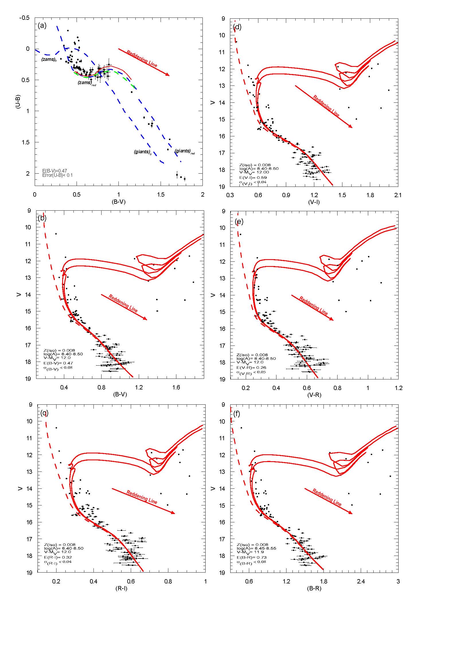
Figure S7: Panel (a): the $(U$–$B,B$–$V)$ diagram of NGC 1857. Panels (b)–(f): CM diagrams of $(V,B$–$V)$, $(V,R$–$I)$, $(V,V$–$I)$, $(V,V$–$R)$, and $(V,B$–$R)$. The symbols are the same as Fig. 1 and Figs. 2–3.

Figure S8: Panel (a): the $(U$–$B,B$–$V)$ diagram of NGC 7142. Panels (b)–(f): CM diagrams of $(V,B$–$V)$, $(V,R$–$I)$, $(V,V$–$I)$, $(V,V$–$R)$, and $(V,B$–$R)$. The symbols are the same as Fig. 1 and Figs. 2–3; the B​S candidates are marked with open squares.

Figure S9: Panel (a): the $(U$–$B,B$–$V)$ diagram of Be 73. Panels (b)–(f): CM diagrams of $(V,B$–$V)$, $(V,R$–$I)$, $(V,V$–$I)$, $(V,V$–$R)$, and $(V,B$–$R)$. The symbols are the same as Fig. 1 and Figs. 2–3.

Figure S16: Panel (a): the $(U$–$B,B$–$V)$ diagram of NGC 2186. Panels (b)–(f): CM diagrams of $(V,B$–$V)$, $(V,R$–$I)$, $(V,V$–$I)$, $(V,V$–$R)$, and $(V,B$–$R)$. The symbols are the same as Fig. 1 and Figs. 2–3.

Figure S17: Panel (a): the $(U$–$B,B$–$V)$ diagram of Haf 08. Panels (b)–(f): CM diagrams of $(V,B$–$V)$, $(V,R$–$I)$, $(V,V$–$I)$, $(V,V$–$R)$, and $(V,B$–$R)$. The symbols are the same as Fig. 1 and Figs. 2–3.

Figure S18: Panel (a): the $(U$–$B,B$–$V)$ diagram of NGC 2304. Panels (b)–(f): CM diagrams of $(V,B$–$V)$, $(V,R$–$I)$, $(V,V$–$I)$, $(V,V$–$R)$, and $(V,B$–$R)$. The symbols are the same as Fig. 1 and Figs. 2–3.

Figure S19: Panel (a): the $(U$–$B,B$–$V)$ diagram of NGC 2360. Panels (b)–(f): CM diagrams of $(V,B$–$V)$, $(V,R$–$I)$, $(V,V$–$I)$, $(V,V$–$R)$, and $(V,B$–$R)$. The symbols are the same as Fig. 1 and Figs. 2–3.

References

- Akkaya et al. (2010) Akkaya, İ., Schuster, W. J., Michel, R., Chavarría-K, C., Moitinho, A., Vázquez, R. & Karataş, Y. 2010, RMxAA, 46, 385 (A10)
- Ann et al. (2002) Ann, H.B., Leo, S.H., Sung, H., Lee, M.G., Kim, S.L., Chun, M. Y., Jeon, Y. B., Park, B. G., Yuk, I. S., 2002, AJ, 123, 905
- Arce & Goodman (1999) Arce, H. G., & Goodman, A. A. 1999., ApJ, 512, L135
- Asplund et al. (2009) Asplund, M., Sauval, A.J., Scott, P., 2009, ARA&A, 47, 481
- Babu (1989) Babu, G.S.D., 1989, JApA, 10, 295
- Bahcall & Soneira (1980) Bahcall, J.N., & Soneira, R.M., 1980, ApJ, 238, 17
- Barbaro et al. (1969) Barbaro, G., Dallaporta, N., Fabris, G., 1969, Ap&SS, 3, 123
- Becker et al. (1976) Becker, W., Svolopoulos, S.N., Fang, Ch., 1976, Kataloge photographischer und photoelektrischer Helligkeiten von 25 galaktischen Sternhaufen im RGU- und UcBV-System
- Bellazzini et al. (2004) Bellazzini, M., Ibata, R.A, Monaco, L., Martin, N.F., Irwin, M.J., Lewis, G.F., 2004, MNRAS, 354, 1263
- Bertelli et al. (1994) Bertelli, G., Bressan, A., Chiosi, C., Fagotto, F., & Nasi, E. 1994, A&AS, 106, 275
- Bonatto & Bica (2007) Bonatto, Ch., Bica, E., 2007, A&A, 473, 445
- Bonifacio et al. (2000) Bonifacio, P., Monai, S., & Beers, T. C. 2000, AJ, 120, 2065
- Brunthaler et al. (2011) Brunthaler, A., Reid, M.J., Menten, K.M., et.al. 2011, AN, 332, No.5, 461
- Caffau et al. (2009) Caffau, E., Maiorca, E., Bonifacio, P., Faraggiana, R., Steffen, M., Ludwig, H.G., Kamp, I., Busso, M., 2009, A&A, 498, 877
- Cameron (1985) Cameron, L. M. 1985, A&A, 147, 47
- Camargo et al. (2009) Camargo, D., Bonatto, C., Bica, E., 2009, A&A, 508, 211
- Cambresy et al. (2005) Cambresy, L., Jarett, T.H., Beichman, C.A., 2005, A&A, 435, 131
- Canterna et al. (1986) Canterna, R., Geisler, D., Harris, H.C., Olszewski, E., Schommer, R., 1986, AJ, 92, 79
- Carney (2001) Carney, B. 2001, Star Clusters, Saas-Fee Advanced Course 28, Lecture Notes 1998, Swiss Society for Astrophysics and Astronomy, eds. L. Labhardt and B. Binggeli (Berlin: Springer-Verlag) pp. 1-222
- Carraro & Chiosi (1994) Carraro, G., Chiosi, C., 1994, A&A, 287, 761
- Carraro et al. (1998) Carraro, G., Ng, Y.K., Portinari, L., 1998, MNRAS, 296, 1045
- Carraro & Vallenari (2000) Carraro, G., Vallenari, A., 2000, A&AS, 142, 59
- Carraro et al. (2005) Carraro, G., Geisler, D., Moitinho, A., Baume, G., Vazquez, R.A., 2005, A&A, 442, 917
- Carraro et al. (2007) Carraro, G., Geisler, D., Villanova, S., Frinchaboy, P.M., Majewski, S.R., 2007, A&A, 476
- Carraro et al. (2008) Carraro, G., Moitinho, A., Vazquez, R.A., 2008, MNRAS, 385, 1597
- Carraro et al. (2010a) Carraro, G., Vazquez, R.A., Costa, E., Perren, G., Moitinho, A., 2010a, AJ, 718, 683
- Carraro et al. (2010b) Carraro, G., Costa, E., Ahumada, J.A., 2010b, AJ, 140, 954
- Chen et al. (1999) Chen, B., Figueras, F., Torra, J., Jordi, C, Luri, X., Galadi-Enr quez, D., 1999, A&A, 352, 459
- Chen et al. (2003) Chen, L., Hou, J.L., Wang, J.J., 2003, AJ, 125, 1397
- Claret et al. (2003) Claret, A., Paunzen, E., Maitzen, H.M., 2003, A&A, 412, 91
- Claria et al. (1989) Claria, J.J., Lapasset, E., Minniti, D., 1989, A&AS, 78, 363
- Claria et al. (1999) Claria, J.J., Mermillod, J. C., Piatti, A.E., 1999, A&AS, 134, 301
- Claria et al. (2008) Claria, J.J., Piatti, A.E., Mermillod, J. C., Palma, T., 2008, AN, 329, 609
- Clem & Landoldt (2013) Clem, J. L., Landoldt, A., 2013, AJ, 146, 88
- Crinklaw & Talbert (1991) Crinklaw, G., Talbert, F.D., 1991, PASP, 103, 536
- Cuffey (1940) Cuffey, J., 1940, ApJ, 92,303
- Dias et al. (2002) Dias, W. S., Alessi, B. S., Moitinho, A., & Lépine, J. R. D., 2002, A&A, 389, 871
- Dias et al. (2012) Dias, W. S., Alessi, B. S., Moitinho, A., & Lépine, J. R. D., 2012, 2010yCat, VizieR On-line Data Catalog: B/ocl.
- Durgapal et al. (2001) Durgapal, A.K., Pandey, A.K., Mohan, V., 2001, A&A, 372, 71
- Eggen (1968) Eggen, O.J., 1968, ApJ, 152, 83
- Fenkart et al. (1972) Fenkart, R.P., Buser, R., Ritter, H., Schmitt, H., Steppe, H., Wagner, R., Wiedemann, D., 1972, A&AS, 7, 487
- Friel & Janes (1993) Friel, E.D. & Janes, K.A., 1993, A&A, 267, 75
- Friel et al. (1995) Friel, E.D., 1995, ARA&A, 33, 381
- Friel et al. (2002) Friel, E.D., Janes, K.A., Tavarez, M., Scott, J., Katsanis, R., Lotz, J., Hong, L., Miller, N., 2002, AJ, 124, 2693
- Geisler et al. (1991) Geisler, D., Claria, J.J., Dante, M., 1991, AJ, 102, 1836
- Geisler et al. (1992) Geisler, D., Claria, J.J., Dante, M., 1992, AJ, 104, 1892
- Gieles et al. (2006) Gieles, M., Portegies-Zwart, S., Athanassoula, E., Baumgardt, H., Lamers, H.J.G.L.M., Sipior, M, Leenaarts, J., 2006, MNRAS, 371, 793
- Gim et al. (1998) Gim, M., Vandenberg, D.A., Stetson, P., Hesser, J., Zurek, D.R., 1998, PASP, 110, 1318
- Girardi et al. (2000) Girardi, L., Bressan, A., Bertelli, G., & Chiosi, C., 2000, A&AS, 141, 371 (http://pleiadi.pd.astro.it)
- Groenewegen (2008) Groenewegen, M.A.T., 2008, A&A, 488, 935
- Hamdani et al. (2000) Hamdani, S., North, P., Mowlari, N., Raboud, D., Mermillod, J. C., 2000, A&A, 360, 509
- Hardie (1962) Hardie, R. H., 1962, in ”Photometric Reductions”, chapter 8 of Astronomical Techniques , edited by W. A. Hiltner, from the series Stars and Stellar Systems , vol III, general editor G. P. Kuiper and associated general editor B. M. Middlehurst, University of Chicago Press, ISBN 0-226-45963-2
- Hasegawa et al. (2008) Hasegawa, T., Sakamoto, T., Malasan, H.L., 2008, PASJ, 60, 1267
- Haywood (2008) Haywood, M., 2008, MNRAS, 388, 1175
- Hoag et al. (1961) Hoag, A.A., Johnson, H. L., Iriarfe, B., Mitchell, R., Hallam, K.L., Sharpless, S., 1961, Publication of the U.S. Naval Obeservatory 2nd Ser., 17, 1
- Houdek & Gough (2011) Houdek, G., Gough, D.O., 2011, MNRAS, 418, 1217
- Howell (1989) Howell, S.B., 1989, PASP, 101, 616
- Howell (1990) Howell, S.B., 1990, in ASP Conf. Ser. 8, CCDs in Astronomy, ed. G.H. Jacoby (San Francisco: ASP), 312
- Huestamendia et al. (1991) Huestamendia, G., del Rio, G., Mermillod J. C., 1991, A&AS, 87, 153
- Jacobson et al. (2008) Jacobson, H., Friel, E.D., Pilachowski C.A., 2008, AJ, 135, 2341
- Jacobson et al. (2011) Jacobson, H., Pilachowski, C.A., Friel E.D., 2011, AJ, 142, 59
- Johnson et al. (1966) Johnson, H.L., Mitchell, R.I., Iriart, B., and Wisniewski, W.Z., 1966, Comm. Lunar and Planet. Labor., University of Arizona 6, No:92,85
- Joshii (2005) Joshii, Y.C., 2005, MNRAS, 362, 1259
- Karataş & Schuster (2006) Karataş, Y., Schuster W.J., 2006, MNRAS, 371, 1793
- King (1952a) King, I., 1952a, ApJ, 115, 580
- King (1952b) King, I., 1952b, AJ, 57, 253
- Landolt (1983) Landolt, A. U., 1983, AJ, 88, 439
- Landolt (1992) Landolt, A. U., 1992, AJ, 104, 340
- Lata et al. (2010) Lata, S., Pandey, A.K., Kumar, B., Bhatt, H., Pace, G., Sharma, S., 2010, AJ, 139, 378
- Lepine et al. (2011) Lepine, J.R.D., Cruz, P. Scarano, S., Barros, D.A., Dias, W.S., Pompeia, L., Andrievsky S.M., Garraro G., Famaey B., 2011, MNRAS, 417, 698
- Lyngaå (1987) Lynga, G., Computer Based Catalogue of Open Cluster Data, Observatoire de Strasbourg, Centre de Données Stellaires, Strasbourg,1987, å.
- Maciejewski & Niedzielski (2007) Maciejewski, G., Niedzielski, A., 2007, A&A, 467, 1065
- Magrini et al. (2009) Magrini, L., Sestio, P., Randich, S., Galli, D., 2009, A&A, 494, 95
- Marigo et al. (2008) Marigo, P., Girardi, L., Bressan, A., Groenewegen, M. A. T., Silva, L., & Granato, G. L., 2008, A&A, 482, 883 (M08)
- Martin et al. (2004) Martin, N.F., Ibata, R.A., Bellazzini, M., Irwin, M.J., Lewis, G.F., Dehnen, W., 2004, MNRAS, 348, 12
- McFarland (2010) McFarland, J., 2010, BSc Thesis, Universidad Autónoma de Baja California, México (e-mail to bibens@astrosen.unam.mx)
- Melbourne (1959) Melbourne, W.G., 1959, PhD. thesis, Calif. Inst. of Tech.
- Melbourne (1960) Melbourne, W.G., 1960, ApJ, 132, 101
- Mermilliod (1992) Mermilliod,, J.C., 1992, Bull. Inform, CDS, 40, 115
- Michel (2014) Michel, R., 2014, in preparation
- Mitchell (1960) Mitchell, R. I., 1960, ApJ, 132,68
- Moffat & Vogt (1975) Moffat, A.F.J., Vogt N., 1975, A&AS, 20, 85
- Moitinho (2010) Moitinho, A., 2010, Star clusters: basic galactic building blocks, Proceedings IAU Symposium No.266, eds. R.de Grijs & J.R.D. Lepine
- Momany et al. (2006) Momany, Y., Zaggia, S., Gilmore, G., Piotto, G., Carraro, G., Bedin, L. R., de Angeli, F., 2006, A&A, 451, 515
- Netopil et al. (2007) Netopil, M., Paunzen, E., Maitzen, H.M., Pintado, O.I., Claret, A., Miranda, L.F., Iliev, Kh. I., Casanova, V., 2007, A&A, 462, 591
- Newberg et al. (2002) Newberg, H.J. et al., 2002, ApJ, 569, 245
- Ortolani et al. (2005) Ortolani, S., Bica, E., Barbuy, B., Zoccali, M., 2005, A&A, 429, 607
- Pandey et al. (2003) Pandey, A.K., Upadhyay, K., Nakada, Y., Ogura, K., 2003, A&A, 397, 191
- Park & Lee (1999) Park, H.S., Lee, M.G., 1999, MNRAS, 304, 883
- Paunzen & Netopil (2006) Paunzen, E., & Netopil, M. 2006, MNRAS, 371, 1641
- Paunzen et al. (2010) Paunzen, E., Heiter, U., Netopil, M., & Soubiran, C., 2010, A&A, 517, 32
- Peniche et al. (1990) Peniche, R., Peña, J.H., Díaz Martinez, S.H., Gómez, T., 1990, RMxAA, 20, 127
- Phelps et al. (1994a) Phelps, R.L., Jane,s K.A., Montgomery, K.A., 1994a, AJ, 107, 1079
- Phelps & Janes (1994b) Phelps, R.L., Janes, K.A., 1994b, ApJS, 90, 31
- Piatti et al. (1995) Piatti, A.E., Claria, J.J., Abadi, M.G., 1995, AJ, 110, 2813
- Piatti et al. (2008) Piatti, A.E., Claria, J.J., Parisi, M.C., Ahumada, A.V., 2008, Balt A, 17, 67
- Piskunov et al. (2008) Piskunov, A.E., Kharchenko, N.V., Schilbach, E., Roser, S., Scholz, R.-D., Zinnecker, H., 2008, A&A, 487, 557
- Salaris et al. (2004) Salaris, M., Weiss, A., Percival, S.M., 2004, A&A, 414, 163
- Sandage (1969) Sandage, A. 1969, ApJ, 158, 1115
- Scarano & Lepine (2013) Scarano, S., Lepine, J.R.D., 2013, MNRAS, 428, 625
- Schlegel et al. (1998) Schlegel, D.J., Finkbeiner, D. P., & Davis, M., 1998, ApJ, 500, 525
- Schmidt-Kaler (1982) Schmidt-Kaler, Th. 1982, in Landolt-Bornstein, Numerical Data and Functional Relationships in Science and Technology, New Series, Group VI, Vol.2b, eds. K. Schaifers & H. H. Voigt (Berlin: Springer), p. 14 (SK82)
- Schönrich & Binney (2009) Schönrich, R., Binney, J., 2009, MNRAS, 396, 203
- Schuster et al. (2004) Schuster, W. J., Beers, T. C., Michel, R., Nissen, P. E., & García, G., 2004, A&A, 422, 527
- Schuster et al. (2007) Schuster,, W. J., Michel, R., Dias, W., Tapia-Peralta, T., Vázquez, R., Macfarland J., Chavarría, C., Santos, C., & Moitinho, A. 2007, Galaxy Evolution Across the Hubble Time, eds. F. Combes and J. Palou, Proceedings of the International Astronomical Union, IAU Symposium No. 235, (Cambridge, United Kingdom: Cambridge University Press), p. 331
- Schuster & Parrao (2001) Schuster, W. J., Parrao, L., 2001, RevMexAA, 37, 187
- Stetson (1987) Stetson, P. B., 1987, PASP, 99, 191
- Stetson (1990) Stetson, P. B., 1990, PASP, 102, 932
- Tadross (2003) Tadross, A.L., 2003, NewAst, 8, 737
- Tadross (2008) Tadross, A.L., 2008, MNRAS, 389, 285
- Tapia et al. (2010) Tapia, M. T., Schuster, W. J., Michel, R., Chavarría-K, C., Dias, W. S., Vázquez, R., & Moitinho, A. 2010, MNRAS, 401, 621 (T10)
- Twarog et al. (1997) Twarog, B.A., Ashman, K.M., Anthony-Twarog, B.J., 1997, AJ, 114, 2556
- Yi et al. (2003) Yi, S.K., Kim, Y.C., Demarque, P., 2003, ApJS, 144, 259
- Yong et al. (2005) Yong, D., Carney, B., Teixera de Almeida, M.L., 2005, AJ, 130, 597
- Yong et al. (2012) Yong, D., Carney, B., Friel, E., 2012, AJ, 144, 95
- Zwitter et al. (2008) Zwitter, T. et al., 2008, AJ, 136, 421