A stabilized nonconforming finite element method for the elliptic Cauchy problem

Abstract

In this paper we propose a nonconforming finite element method for the solution of the ill-posed elliptic Cauchy problem. We prove error estimates using continuous dependence estimates in the $L^{2}$-norm. The effect of perturbations in data on the estimates is investigated. The recently derived framework from [8, 9] is extended to include the case of nonconforming approximation spaces and we show that the use of such spaces allows us to reduce the amount of stabilization necessary for convergence, even in the case of ill-posed problems.

1 Introduction

We consider the Cauchy problem for Poisson’s equation in a bounded domain. This problem is known to be severely ill-posed in the sense of Hadamard [16, 5, 2]. The ill-posedness makes numerical approximation challenging and different regularization methods have been proposed, such as Tikhonov regularization [26] or the quasi reversibility method introduced by Lattès and Lions [23].

Various finite element approaches for the solution of the elliptic Cauchy problem have been suggested in the litterature. Some are based on standard Galerkin formulations, but rely on structured meshes or a special form of the continuous problem for stability [15, 24, 25]. Some use the above mentioned regularization techniques to ensure stability [3, 4, 6, 7, 13] a related approach is to recast the problem as a minimization problem [11, 18, 17], possibly with regularization.

The objective of the present work is to draw on the ideas of [8, 9] and propose a consistent stabilization of a non-conforming finite element method. The upshot is that the use of nonconforming elements allows us to use a standard stabilization operators known from previous works on well-posed problems [19, 20, 10] for stability. Indeed we only need to apply a penalty on the jump of the approximate solution over element faces. The structure of the method bears some ressemblance to that introduced in [6], but the stabilizing terms in our case are consistent for exact solutions in $H^{1}(\Omega)$. The key observation here is that the functional to be minimized has on effect only on the discrete space, indeed it is zero for any function in $H^{1}$. The associated Euler-Lagrange equations result in a consistent stabilized finite element method.

The fact that the stabilization is consistent allows us to derive error estimates using discrete stability and the continuous dependence on data of the partial differential equation. We follow an approach similar to that suggested in [9], but in this case an inf-sup condition is necessary for the discrete stability. The error bound is on a posteriori form, using a residual quantity together with the continuous dependence. Thanks to the primal/adjoint stabilization the residual terms can be shown to be optimally convergent independent of the stability of the underlying problem, for sufficiently smooth solutions.

We also show how perturbed data can be introduced in the analysis and discuss how a posteriori control of the mesh refinement may include the effect of perturbations, provided their magnitude is known.

The problem that we are interested in takes the form: find $u:\Omega\mapsto\mathbb{R}$ such that

$$\left\{\begin{array}[]{rcl}-\Delta u&=&f,\mbox{ in }\Omega\\ u&=&0\mbox{ on }\Gamma_{D}\\ \nabla u\cdot n&=&\psi\mbox{ on }\Gamma_{C}\end{array}\right.$$ (1.1)

where $\Omega\subset\mathbb{R}^{d}$, $d=2,3$ is a convex polyhedral (polygonal) domain and $\Gamma_{C},\,\Gamma_{D}$ denote simply connected parts of the boundary $\partial\Omega$, such that $\Gamma_{C}\subset\Gamma_{D}\subset\partial\Omega$. We denote the complement to the Dirichlet boundary $\Gamma_{D}^{\prime}:=\partial\Omega\setminus\Gamma_{D}$ and the complement of the Cauchy boundary $\Gamma_{C}^{\prime}:=\partial\Omega\setminus\Gamma_{C}$. For simplicity we will assume that both $\Gamma_{C}$, $\Gamma_{D}$ and $\Gamma_{D}^{\prime}$ have strictly positive $(d-1)$-measure. The practical interest of (1.1) stems from engineering problems where the exact boundary condition is unknown on part of the boundary, but additional measurements $\psi$ of the fluxes are available on the accessible boundary $\Gamma_{D}$. It is then reasonable to assume that there exists a unique solution with a certain regularity and then prove convergence of the numerical method under these assumptions. This is the approach we will take below. To this end we assume that $f\in L^{2}(\Omega)$, $\psi\in H^{\frac{1}{2}}(\Gamma)$ and that a unique $u\in H^{2}(\Omega)$ satisfies (1.1).

For the derivation of a weak formulation we introduce the spaces $V:=\{v\in H^{1}(\Omega):v|_{\Gamma_{D}}=0\}$ and $W:=\{v\in H^{1}(\Omega):v|_{\Gamma_{C}^{\prime}}=0\},$ both equipped with the $H^{1}$-norm and with dual spaces denoted by $V^{\prime}$ and $W^{\prime}$.

Using these spaces we obtain a weak formulation: find $u\in V$ such that

$$a(u,w)=l(w)\quad\forall w\in W,$$ (1.2)

where

$$a(u,w)=\int_{\Omega}\nabla u\cdot\nabla w~{}\mbox{d}x,$$

and

$$l(w):=\int_{\Omega}fw~{}\mbox{d}x+\int_{\Gamma_{C}}\psi\,w~{}\mbox{d}s.$$

We will use the notation $(\cdot,\cdot)_{X}$ for the $L^{2}$-scalar product over $X$ and for the associated norm we write $\|x\|_{X}:=(x,x)_{X}^{\frac{1}{2}}$. The $H^{s}$-norm will be denoted by $\|\cdot\|_{H^{s}(\Omega)}$ and we identify the norms on $V$ and $W$ with the $H^{1}$-norm, $\|\cdot\|_{V}=\|\cdot\|_{W}=\|\cdot\|_{H^{1}(\Omega)}$. Observe that we may not assume that the problem is well-posed for general $l(\cdot)\in W^{\prime}$. Indeed since $u\not\in W$ coercivity fails and inf-sup stability does not hold either in general [5].

1.1 Continuous dependence on data

The problem (1.1) is ill-posed and for our analysis we will only use a continuous dependence result linking the size of some functional to the solution to the size of data. Consider the functional $j:V\mapsto\mathbb{R}$. Let $\Xi:\mathbb{R}^{+}\mapsto\mathbb{R}^{+}$ be a continuous, monotone increasing function with $\lim_{x\rightarrow 0^{+}}\Xi(x)=0$. The continuous dependence that we will assume then takes the form.

If for $$\epsilon>0 \|l\|_{W^{\prime}}\leq\epsilon \epsilon |j(u)|\leq\Xi(\epsilon).$$, there holds in (1.2) then, for small enough, (1.3)

It is known [2, Theorems 1.7 and 1.9] that if there exists a solution $u\in H^{1}(\Omega)$, with $E:=\|u\|_{H^{1}(\Omega)}$ to (1.1), a continuous dependence of the form (1.3) holds for $0<\epsilon<1$ and

$$\begin{array}[]{l}\mbox{$j(u):=\|u\|_{L^{2}(\omega)}$, $\omega\subset\Omega:\,\mbox{dist}(\omega,\partial\Omega)=:d_{\omega,\partial\Omega}>0$}\\[8.53581pt] \mbox{ with $\Xi(x)=C(E)x^{\varsigma}$, $C(E)>0$, $\varsigma:=\varsigma(d_{\omega,\partial\Omega})\in(0,1)$}\end{array}$$ (1.4)

and for

$$\begin{array}[]{l}\mbox{$j(u):=\|u\|_{L^{2}(\Omega)}$ with $\Xi(x)=C_{1}(E)(|\log(x)|+C_{2}(E))^{-\varsigma}$}\\[8.53581pt] \mbox{ with $C_{1}(E),C_{2}(E)>0$, $\varsigma\in(0,1)$.}\end{array}$$ (1.5)

The constants above also depend on the geometry of the problem. Note that to derive these results $l(\cdot)$ is first associated with its Riesz representant in $W$ (c.f. [2, equation (1.31)] and discussion.)

2 The nonconforming stabilized method

Let $\{\mathcal{T}_{h}\}_{h}$ denote a family of shape regular and quasi uniform tesselations of $\Omega$ into nonoverlapping simplices, such that for any two different simplices $\kappa$, $\kappa^{\prime}\in\mathcal{T}_{h}$, $\kappa\cap\kappa^{\prime}$ consists of either the empty set, a common face or a common vertex. The diameter of a simplex $\kappa$ will be denoted $h_{\kappa}$ and the outward pointing normal $n_{\kappa}$. The family $\{\mathcal{T}_{h}\}_{h}$ is indexed by the maximum element-size of $\mathcal{T}_{h}$, $h:=\max_{\kappa\in\mathcal{T}_{h}}h_{\kappa}$. We denote the set of element faces in $\mathcal{T}_{h}$ by $\mathcal{F}$ and let $\mathcal{F}_{i}$ denote the set of interior faces and $\mathcal{F}_{\Gamma}$ the set of faces in some $\Gamma\subset\partial\Omega$. To each face $F\in\mathcal{F}$ we associate the mesh parameter $h_{F}:=\mbox{diam}(F)$. We will assume that the mesh is fitted to the subsets of $\partial\Omega$ representing the boundary conditions $\Gamma_{D}$ and $\Gamma_{C}$, so that the boundaries of these subsets coincide with element boundaries. To each face $F$ we associate a unit normal vector, $n_{F}$. For interior faces its orientation is arbitrary, but fixed. On the boundary $\partial\Omega$ we identify $n_{F}$ with the outward pointing normal of $\Omega$. We define the jump over interior faces $F\in\mathcal{F}_{i}$ by $[v]|_{F}:=\lim_{\epsilon\rightarrow 0^{+}}(v(x|_{F}-\epsilon n_{F})-v(x|_{F}+\epsilon n_{F}))$ and for faces on the boundary, $F\in\partial\Omega$, we let $[v]|_{F}:=v|_{F}$. Similarly we define the average of a function over an interior face $F$ by $\{v\}|_{F}:=\tfrac{1}{2}\lim_{\epsilon\rightarrow 0^{+}}(v(x|_{F}-\epsilon n_{F})+v(x|_{F}+\epsilon n_{F}))$ and for $F$ on the boundary we define $\{v\}|_{F}:=v|_{F}$. The classical nonconforming space of piecewise affine finite element functions (see [12]) then reads

$$X_{h}^{\Gamma}:=\{v_{h}\in L^{2}(\Omega):\int_{F}[v_{h}]~{}\mbox{d}s=0,\,\forall F\in\mathcal{F}_{i}\cup\mathcal{F}_{\Gamma}\mbox{ and }v_{h}|_{\kappa}\in\mathbb{P}_{1}(\kappa),\,\forall\kappa\in\mathcal{T}_{h}\}$$

where $\mathbb{P}_{1}(\kappa)$ denotes the set of polynomials of degree less than or equal to one restricted to the element $\kappa$ and $\Gamma$ denotes some portion of the boundary $\partial\Omega$ consisting of a union of a subset of boundary element faces. We may then define the spaces $V_{h}:=X_{h}^{\Gamma_{D}}$ and $W_{h}:=X_{h}^{\Gamma_{C}^{\prime}}$. We recall the interpolation operator $r_{h}:H^{1}(\Omega)\rightarrow X_{h}^{\Gamma}$ defined by the relation

$$\overline{\{r_{h}v\}}|_{F}:=|F|^{-1}\int_{F}\{r_{h}v\}~{}\mbox{d}s=|F|^{-1}\int_{F}u~{}\mbox{d}s$$

for every $F\in\mathcal{F}$ and with $|F|$ denoting the $(d-1)$-measure of $F$. It is conventient to introduce the broken norms

$$\|x\|_{h}^{2}:=\sum_{\kappa\in\mathcal{T}_{h}}\|x\|_{\kappa}^{2}\mbox{ and }\|x\|_{1,h}^{2}:=\|x\|_{h}^{2}+\|\nabla x\|_{h}^{2}.$$

The following inverse and trace inequalities are well known

$$\begin{array}[]{rcl}\|v\|_{\partial\kappa}\leq C_{t}(h_{\kappa}^{-\frac{1}{2}}\|v\|_{\kappa}+h_{\kappa}^{\frac{1}{2}}\|\nabla v\|_{\kappa}),\forall v\in H^{1}(\kappa)\\[8.53581pt] h_{\kappa}\|\nabla v_{h}\|_{\kappa}+h_{\kappa}^{\frac{1}{2}}\|v_{h}\|_{\partial\kappa}\leq C_{i}\|v_{h}\|_{\kappa},\quad\forall v_{h}\in X_{h}^{\Gamma}.\end{array}$$ (2.1)

Using the inequalities of (2.1) and standard approximation results from [12] it is straightforward to show the following approximation results of the interpolant $r_{h}$

$$\begin{array}[]{rcl}\|u-r_{h}u\|+h\|\nabla(u-r_{h}u)\|_{h}&\leq&Ch^{t}|u|_{H^{t}(\Omega)}\\[8.53581pt] \|h^{-\frac{1}{2}}(u-r_{h}u)\|_{\mathcal{F}}+\|h^{\frac{1}{2}}\nabla(u-r_{h}u)\cdot n_{F}\|_{\mathcal{F}}&\leq&Ch^{t-1}|u|_{H^{t}(\Omega)}\end{array}$$ (2.2)

where $t\in\{1,2\}$. It will also be useful to bound the $L^{2}$-norm of the interpolant $r_{h}$ by its values on the element faces. To this end we prove a technical lemma.

Lemma 2.1.

For any function $v_{h}\in X_{h}^{\Gamma}$ there holds

$$\|h^{-1}v_{h}\|_{\Omega}\leq c_{\mathcal{T}}\left(\sum_{F\in\mathcal{F}}h^{-1}_{F}\|\overline{\{v_{h}\}}\|^{2}_{F}\right)^{\frac{1}{2}}$$

Proof.

It follows by norm equivalence of discrete spaces on the reference element and a scaling argument (under the assumption of shape regularity) that for all $\kappa\in\mathcal{T}_{h}$

$$\|v_{h}\|^{2}_{\kappa}\leq C\sum_{\begin{subarray}{c}F\in\partial\kappa\end{subarray}}h_{F}\|\overline{v}_{h}\|_{F}^{2}.$$ (2.3)

The claim follows by shape regularity and by summing over the elements of $\mathcal{T}_{h}$ and recalling that $\|\overline{v}_{h}\|_{F}^{2}=\|\overline{\{v_{h}\}}\|_{F}^{2}$. ∎

Following [6, 8] the formulation may now be written: find $(u_{h},z_{h})\in V_{h}\times W_{h}$ such that,

$$\begin{array}[]{rcl}a_{h}(u_{h},w_{h})-s_{W}(z_{h},w_{h})&=&l(w_{h})\\[8.53581pt] a_{h}(v_{h},z_{h})+s_{V}(u_{h},v_{h})&=&0\end{array}$$ (2.4)

for all $(v_{h},w_{h})\in V_{h}\times W_{h}$. Here the bilinear forms are defined by

$$a_{h}(u_{h},w_{h})=\sum_{\kappa\in\mathcal{T}_{h}}\int_{\kappa}\nabla u_{h}\cdot\nabla w_{h}~{}\mbox{d}x,$$

$$s_{W}(z_{h},w_{h}):=\sum_{\kappa\in\mathcal{T}_{h}}\int_{\kappa}\gamma_{W}\nabla z_{h}\cdot\nabla w_{h}~{}\mbox{d}x$$ (2.5)

or

$$s_{W}(z_{h},w_{h}):=\sum_{F\in\mathcal{F}_{i}\cup\mathcal{F}_{\Gamma_{C}^{\prime}}}\int_{F}\gamma_{W}h_{F}^{-1}[z_{h}][w_{h}]~{}\mbox{d}s$$ (2.6)

and finally

$$s_{V}(u_{h},v_{h}):=\sum_{F\in\mathcal{F}_{i}\cup\mathcal{F}_{\Gamma_{D}}}\int_{F}\gamma_{V}h_{F}^{-1}[u_{h}][v_{h}]~{}\mbox{d}s.$$ (2.7)

We also propose the compact form: find $(u_{h},z_{h})\in\mathcal{V}_{h}:=V_{h}\times W_{h}$ such that,

$$A_{h}[(u_{h},z_{h}),(v_{h},w_{h})]=l(w_{h})$$

for all $(v_{h},w_{h})\in\mathcal{V}_{h}$. The bilinear form is then given by

$$A_{h}[(u_{h},z_{h}),(v_{h},w_{h})]:=a_{h}(u_{h},w_{h})-s_{W}(z_{h},w_{h})+a_{h}(v_{h},z_{h})+s_{V}(u_{h},v_{h}).$$

Observe that for (2.5), by Poincaré’s inequality there exists $c_{1},c_{2}>0$ so that

$$c_{1}\gamma_{W}^{\frac{1}{2}}\|w_{h}\|_{1,h}\leq s_{W}(w_{h},w_{h})^{\frac{1}{2}}\leq c_{2}\gamma_{W}^{\frac{1}{2}}\|w_{h}\|_{1,h},\forall w_{h}\in W_{h}.$$

This norm equivalence is important for stability when there are perturbations in data (see Lemma 4.3). For the weaker adjoint stabilization (2.6) only the upper bound holds. For the first part of the analysis (sections 3-4) the stability obtained by (2.6) is sufficient and the analysis is identical. In Section 4.1 where perturbed data are considered the two approaches lead to slightly different estimates. This operator has the advantage of being adjoint consistent, but since duality arguments are not used herein this has no impact on the results presented below. The stabilization (2.5) will be considered in the analysis, but we will outline in remarks how the arguments change if (2.6) is used. We will then compare the behavior of the two operators numerically.

We end this section by proving two technical Lemmas that will be useful in the analysis. Using the regularity assumptions on the data in $l(w)$ it is straightforward to show that the formulation satisfies the following weak consistency

Lemma 2.2.

(Weak consistency) Let $u$ be the solution of (1.1), with $f\in L^{2}(\Omega)$ and $\psi\in L^{2}(\Gamma_{C})$ and let $(u_{h},z_{h})\in\mathcal{V}_{h}$ be the solution of (2.4) then, for all $w_{h}\in W_{h}$, there holds,

$$|a_{h}(u_{h}-u,w_{h})-s_{W}(z_{h},w_{h})|\leq\sum_{F\in\mathcal{F}_{i}\cup\mathcal{F}_{\Gamma_{C}^{\prime}}}\inf_{\nu_{h}\in V_{h}}\int_{F}|(\nabla u-\{\nabla\nu_{h}\})\cdot n_{F}||[w_{h}]|~{}\mbox{d}s.$$ (2.8)

Proof.

Multiplying (1.1) with $w_{h}\in W_{h}$ and integrating by parts we have

$$\int_{\Omega}fw_{h}~{}\mbox{d}x=-\int_{\Omega}\Delta uw_{h}~{}\mbox{d}x\\ =-\sum_{\kappa\in\mathcal{T}_{h}}\sum_{\begin{subarray}{c}F\in\partial\kappa\\ F\not\in\Gamma_{C}\end{subarray}}\int_{F}\nabla u\cdot n_{\kappa}w_{h}~{}\mbox{d}s+a_{h}(u,w_{h})-\int_{\Gamma_{C}}\psi w_{h}~{}\mbox{d}s$$ (2.9)

or by rearranging terms

$$a_{h}(u,w_{h})=l(w_{h})+\sum_{\kappa\in\mathcal{T}_{h}}\sum_{\begin{subarray}{c}F\in\partial\kappa\\ F\not\in\Gamma_{C}\end{subarray}}\int_{F}\nabla u\cdot n_{\kappa}w_{h}~{}\mbox{d}s.$$

Using (2.4) we obtain

$$a_{h}(u_{h}-u,w_{h})-s(z_{h},w_{h})=-\sum_{\kappa\in\mathcal{T}_{h}}\sum_{\begin{subarray}{c}F\in\partial\kappa\\ F\not\in\Gamma_{C}\end{subarray}}\int_{F}\nabla u\cdot n_{\kappa}w_{h}~{}\mbox{d}s.$$

By the definition of the finite element space $W_{h}$ on $\Gamma_{C}^{\prime}$ and since every internal face appears twice with different orientation of $n_{\kappa}$ we have for all $\nu_{h}\in V_{h}$,

$$\sum_{\begin{subarray}{c}F\in\partial\kappa\\ F\not\in\Gamma_{C}\end{subarray}}\int_{F}\nabla u\cdot n_{\kappa}w_{h}~{}\mbox{d}s=\sum_{\begin{subarray}{c}F\in\partial\kappa\\ F\not\in\Gamma_{C}\end{subarray}}\int_{F}(\nabla u-\{\nabla\nu_{h}\})\cdot n_{\kappa}~{}w_{h}~{}\mbox{d}s.$$

We now observe that by replacing $w_{h}$ with the jump $[w_{h}]$ we may write the sum over the faces of the mesh, replacing $n_{\kappa}$ by $n_{F}$. The conclusion follows by taking absolute values on both sides and moving the absolute values under the intergral sign creating the desired inequality. ∎

Lemma 2.3.

For any $v\in H^{1}(\Omega)$ and for all $w_{h}\in W_{h}$ there holds

$$a(v-r_{h}v,w_{h})=0.$$

Proof.

By integration by parts we have

$$a(v-r_{h}v,w_{h})=\sum_{\kappa\in\mathcal{T}_{h}}\sum_{F\in\partial\kappa}\int_{F}(v-r_{h}v)\nabla w_{h}\cdot n_{\kappa}~{}\mbox{d}s=0,$$

where the last equality is a consequence of the definition of $r_{h}u$. ∎

3 Stability estimates

The issue of stability of the discrete formulation is crucial since we have no coercivity or inf-sup stability of the continuous formulation (1.2) to rely on. By taking $v_{h}=u_{h}$ and $w_{h}=-z_{h}$, and defining the semi-norm $|v_{h}|_{s_{V}}:=s_{V}(v_{h},v_{h})^{\frac{1}{2}},\,\forall v_{h}\in V_{h}$ and the norm $\|w_{h}\|_{s_{W}}:=s_{W}(w_{h},w_{h})^{\frac{1}{2}},\,\forall w_{h}\in W_{h}$ we obtain the stability estimate

$$|u_{h}|^{2}_{s_{V}}+\|z_{h}\|^{2}_{s_{W}}=-l(z_{h})$$ (3.1)

showing that we have control of $z_{h}$ and of the nonconforming part of the approximation of $u_{h}$. If the stabilization operator (2.6) is used, $\|\cdot\|_{s_{W}}$ is a semi-norm similar to $|\cdot|_{s_{V}}$. The stability (3.1) is of course insufficient for any useful analysis, however we will use it here as a starting point for an inf-sup argument that implies existence of a unique discrete solution. To this end we introduce a mesh-dependent norm

$$|\mspace{-1.0mu}|\mspace{-1.0mu}|v_{h}|\mspace{-1.0mu}|\mspace{-1.0mu}|_{V}:=\gamma^{\frac{1}{2}}_{V}\|h\nabla v_{h}\|_{h}+\gamma^{\frac{1}{2}}_{V}\|h[n_{F}\cdot\nabla v_{h}]\|_{\mathcal{F}_{i}\cup\mathcal{F}_{\Gamma_{C}}}+|v_{h}|_{s_{V}},$$ (3.2)

where

$$\|h^{\frac{1}{2}}[n\cdot\nabla v_{h}]\|_{\mathcal{F}_{i}\cup\mathcal{F}_{\Gamma_{C}}}^{2}:=\sum_{F\in{\mathcal{F}_{i}\cup\mathcal{F}_{\Gamma_{C}}}}h_{F}\|[n_{F}\cdot\nabla v_{h}]\|^{2}_{F}.$$

The following approximation estimate is an immediate consequence of (2.2),

$$|\mspace{-1.0mu}|\mspace{-1.0mu}|v-r_{h}v|\mspace{-1.0mu}|\mspace{-1.0mu}|_{V}\leq C\gamma_{V}^{\frac{1}{2}}h|v|_{H^{2}(\Omega)},\quad\forall v\in H^{2}(\Omega).$$ (3.3)

We will also use the composite norm

$$|\mspace{-1.0mu}|\mspace{-1.0mu}|(u_{h},z_{h})|\mspace{-1.0mu}|\mspace{-1.0mu}|:=|\mspace{-1.0mu}|\mspace{-1.0mu}|u_{h}|\mspace{-1.0mu}|\mspace{-1.0mu}|_{V}+\|z_{h}\|_{s_{W}}.$$

Since Dirichlet boundary conditions are set weakly on $\Gamma_{C}$ in $V_{h}$ and on $\Gamma_{C}^{\prime}$ in $W_{h}$, $|\mspace{-1.0mu}|\mspace{-1.0mu}|(u_{h},z_{h})|\mspace{-1.0mu}|\mspace{-1.0mu}|$ is a norm, when (2.5) is used. When (2.6), the jump of $\nabla z_{h}$ and $\|hz_{h}\|_{1,h}$ can be included in the norm above. We now prove a fundamental stability result for the discretization (2.4).

Theorem 3.1.

Assume that $(\gamma_{V}\gamma_{W})\leq(C_{i}c_{\mathcal{T}})^{-2}$. Then there exists a positive constant $c_{s}$ independent of $\gamma_{V},\,\gamma_{W}$ such that there holds

$$c_{s}|\mspace{-1.0mu}|\mspace{-1.0mu}|(x_{h},y_{h})|\mspace{-1.0mu}|\mspace{-1.0mu}|\leq\sup_{(v_{h},w_{h})\in\mathcal{V}_{h}}\frac{A_{h}[(x_{h},y_{h}),(v_{h},w_{h})]}{|\mspace{-1.0mu}|\mspace{-1.0mu}|(v_{h},w_{h})|\mspace{-1.0mu}|\mspace{-1.0mu}|}.$$

Proof.

First we recall the positivity

$$|x_{h}|_{s_{V}}^{2}+\|y_{h}\|_{s_{W}}^{2}=A_{h}[(x_{h},y_{h}),(x_{h},-y_{h})].$$

Then observe that by integrating by parts in the bilinear form $a_{h}(\cdot,\cdot)$ and using the zero mean value property of the approximation space we have

$$a_{h}(x_{h},w_{h})=\sum_{F\in\mathcal{F}}\int_{F}[n_{F}\cdot\nabla x_{h}]\{w_{h}\}~{}\mbox{d}s.$$

Define the function $\xi_{h}\in W_{h}$ such that for every face $F\in\mathcal{F}_{i}\cup\mathcal{F}_{\Gamma_{C}}$

$$\overline{\{\xi_{h}\}}|_{F}:=\gamma_{V}h_{F}[n_{F}\cdot\nabla x_{h}]|_{F}.$$

This is possible in the nonconforming finite element space since the degrees of freedom may be identified with the average value of the finite element function on an element face. Using Lemma 2.1 we have

$$\|h^{-1}\xi_{h}\|^{2}_{\Omega}\leq c_{\mathcal{T}}^{2}\sum_{F\in\mathcal{F}_{i}\cup\mathcal{F}_{C}}\gamma_{V}^{2}\|h_{F}^{\frac{1}{2}}[n_{F}\cdot\nabla x_{h}]\|_{F}^{2}.$$ (3.4)

Testing with $w_{h}=\xi_{h}$ and $v_{h}=0$ we get

$$\gamma_{V}\|h^{\frac{1}{2}}[\nabla x_{h}\cdot n_{F}]\|_{\mathcal{F}_{i}\cup\mathcal{F}_{\Gamma_{C}}}^{2}=A_{h}[(x_{h},y_{h}),(0,\xi_{h})]+s_{W}(y_{h},\xi_{h}).$$

For the stabilization terms in the right hand side we have the upper bounds, using the inverse inequality (trace inequality if (2.6) is used) (2.1)(ii) and (3.4)

$$s_{W}(y_{h},\xi_{h})\leq\|y_{h}\|_{s_{W}}\|\xi_{h}\|_{s_{W}}\leq C_{i}\|y_{h}\|_{s_{W}}\gamma_{W}^{\frac{1}{2}}\|h^{-1}\xi_{h}\|_{\Omega}\\ \leq C_{i}c_{\mathcal{T}}\|y_{h}\|_{s_{W}}(\gamma_{V}\gamma_{W})^{\frac{1}{2}}\|\gamma_{V}^{\frac{1}{2}}h^{\frac{1}{2}}[n\cdot\nabla x_{h}]\|_{\mathcal{F}_{i}\cup\mathcal{F}_{\Gamma_{C}}}.$$

The consequence of this is that for $\gamma_{V}\gamma_{W}<(C_{i}c_{\mathcal{T}})^{-2}$ there holds

$$\frac{1}{2}\left(|x_{h}|_{s_{V}}^{2}+\|y_{h}\|_{s_{W}}^{2}+\gamma_{V}^{\frac{1}{2}}\|h^{\frac{1}{2}}[n\cdot\nabla x_{h}]\|_{\mathcal{F}_{i}\cup\mathcal{F}_{\Gamma_{C}}}^{2}\right)\\ \leq A_{h}[(x_{h},y_{h}),(x_{h},-y_{h}+\xi_{h})].$$ (3.5)

To include the control of the gradient of $x_{h}$ we use a well-known discrete Poincaré inequality for piecewise constant functions [14]

$$\|\nabla x_{h}\|_{h}^{2}\leq C\sum_{F\in\mathcal{F}_{i}\cup\mathcal{F}_{C}}h_{F}^{-1}\|[\nabla x_{h}]\|_{F}^{2}.$$

The right hand side is now upper bounded by decomposing the jump of the gradient on its normal and tangential part and applying the inverse inequality

$$\|h^{\frac{1}{2}}[(I-n_{F}\otimes n_{F})\nabla x_{h}]\|_{F}\leq C\|h^{-\frac{1}{2}}[x_{h}]\|_{F}$$

in the latter. Relating the right hand side to the quantities in $|\mspace{-1.0mu}|\mspace{-1.0mu}|\cdot|\mspace{-1.0mu}|\mspace{-1.0mu}|_{V}$ already controlled in (3.5), this leads to the upper bound

$$\|\nabla x_{h}\|_{h}\leq Ch^{-1}(\|h^{\frac{1}{2}}[n\cdot\nabla x_{h}]\|_{\mathcal{F}_{i}\cup\mathcal{F}_{\Gamma_{C}}}+\gamma_{V}^{-\frac{1}{2}}|x_{h}|_{s_{V}}).$$

and hence

$$h\gamma_{V}^{\frac{1}{2}}\|\nabla x_{h}\|_{h}\leq C(\gamma_{V}^{\frac{1}{2}}\|h^{\frac{1}{2}}[n\cdot\nabla x_{h}]\|_{\mathcal{F}_{i}\cup\mathcal{F}_{\Gamma_{C}}}+|x_{h}|_{s_{V}}).$$

We may conclude that there exists a positive constant $c_{0}>0$ independent of $\gamma_{V},\,\gamma_{W}$ such that

$$c_{0}|\mspace{-1.0mu}|\mspace{-1.0mu}|(x_{h},y_{h})|\mspace{-1.0mu}|\mspace{-1.0mu}|^{2}\leq A_{h}[(x_{h},y_{h}),(x_{h},-y_{h}+\xi_{h})].$$

To end the proof we need to prove the stability of $\xi_{h}$ in the triple norm. By the triangular inequality

$$|\mspace{-1.0mu}|\mspace{-1.0mu}|(x_{h},-y_{h}+\xi_{h})|\mspace{-1.0mu}|\mspace{-1.0mu}|\leq|\mspace{-1.0mu}|\mspace{-1.0mu}|(x_{h},y_{h})|\mspace{-1.0mu}|\mspace{-1.0mu}|+|\mspace{-1.0mu}|\mspace{-1.0mu}|(0,\xi_{h})|\mspace{-1.0mu}|\mspace{-1.0mu}|.$$

Using now an inverse inequality followed by the argument of (3.4) we arrive at

$$|\mspace{-1.0mu}|\mspace{-1.0mu}|(0,\xi_{h})|\mspace{-1.0mu}|\mspace{-1.0mu}|=\|\xi_{h}\|_{s_{W}}\leq\gamma_{W}^{\frac{1}{2}}C_{i}\|h^{-1}\xi_{h}\|_{\Omega}\leq C_{i}c_{\mathcal{T}}(\gamma_{W}\gamma_{V})^{\frac{1}{2}}|\mspace{-1.0mu}|\mspace{-1.0mu}|x_{h}|\mspace{-1.0mu}|\mspace{-1.0mu}|_{V}\leq|\mspace{-1.0mu}|\mspace{-1.0mu}|(x_{h},y_{h})|\mspace{-1.0mu}|\mspace{-1.0mu}|.$$

This concludes the proof with $c_{s}=c_{0}/2$. ∎

Remark 3.2.

If the stabilization operator defined by equation (2.6) is used, stability of $\|h\nabla y_{h}\|$ may be included using a similar argument. This control of the dual variable is nevertheless weaker than that provided using (2.5).

Corollary 3.3.

The formulation (2.4) admits a unique solution $(u_{h},z_{h})$.

Proof.

The system matrix corresponding to (2.4) is a square matrix and we only need to show that there are no zero eigenvalues. Assume that $l(w_{h})=0$. It then follows by Theorem 3.1 that for any solution $(u_{h},z_{h})$ there holds

$$c_{s}|\mspace{-1.0mu}|\mspace{-1.0mu}|(u_{h},z_{h})|\mspace{-1.0mu}|\mspace{-1.0mu}|\leq\sup_{(v_{h},w_{h})\in\mathcal{V}_{h}}\frac{A_{h}[(u_{h},z_{h}),(v_{h},w_{h})]}{|\mspace{-1.0mu}|\mspace{-1.0mu}|(v_{h},w_{h})|\mspace{-1.0mu}|\mspace{-1.0mu}|}=0,$$

implying that $u_{h}=0$, $z_{h}=0$ which shows that the solution is unique. ∎

4 Error estimates

Even though Theorem 3.1 provides us with a stability estimate for the formulation, the norm is not sufficiently strong to allow for a proof of convergence. Indeed the only notion of stability at our disposal that can allow us to prove error estimates are (1.4) and (1.5). We will follow the approach introduced in [9] and first prove that $|\mspace{-1.0mu}|\mspace{-1.0mu}|(u-u_{h},z_{h})|\mspace{-1.0mu}|\mspace{-1.0mu}|\leq Ch|u|_{H^{2}(\Omega)}$. This tells us that the stabilization terms must vanish at an optimal rate for smooth $u$ and that $\|\nabla u_{h}\|_{h}+\|\nabla z_{h}\|_{h}$ is uniformly bounded as $h\rightarrow 0$. Using this a priori bound we may conclude that the $H^{1}$-conforming part of $u_{h}$ is uniformly bounded in $H^{1}$. This allows us to write the error $u-u_{h}$ as $u-\tilde{u}_{h}+\tilde{u}_{h}-u_{h}=\tilde{e}+e_{h}$, where $\tilde{u}_{h}$ denotes the $H^{1}$-conforming part of $u_{h}$. We may then control the part $\tilde{e}$ using the continuous dependence estimates (1.4) and (1.5), while $e_{h}$ is shown to be bounded by the stabilization.

Proposition 4.1.

Let $u\in H^{2}(\Omega)$ be the solution of (1.1) and $(u_{h},z_{h})\in\mathcal{V}_{h}$ the solution of (2.4). Then

$$|\mspace{-1.0mu}|\mspace{-1.0mu}|(u-u_{h},z_{h})|\mspace{-1.0mu}|\mspace{-1.0mu}|\leq C(\gamma_{V}^{\frac{1}{2}}+c_{s}^{-1}(\gamma_{W}^{-\frac{1}{2}}+\gamma_{V}^{\frac{1}{2}}))h\|u\|_{H^{2}(\Omega)}$$ (4.1)

and

$$\|\nabla u_{h}\|_{h}\leq C(1+c_{s}^{-1}(\gamma_{W}^{-\frac{1}{2}}\gamma_{V}^{-\frac{1}{2}}+1))\|u\|_{H^{2}(\Omega)}.$$ (4.2)

Proof.

Using a triangle inequality and the approximation (3.3) it is sufficient to consider the discrete error $\mu_{h}=u_{h}-r_{h}u$. By Theorem 3.1 we have the stability

$$c_{s}|\mspace{-1.0mu}|\mspace{-1.0mu}|(\mu_{h},z_{h})|\mspace{-1.0mu}|\mspace{-1.0mu}|\leq\sup_{(v_{h},w_{h})\in\mathcal{V}_{h}}\frac{A_{h}[(\mu_{h},z_{h}),(v_{h},w_{h})]}{|\mspace{-1.0mu}|\mspace{-1.0mu}|(v_{h},w_{h})|\mspace{-1.0mu}|\mspace{-1.0mu}|}.$$ (4.3)

Using the formulation and Lemma 2.3 we observe that

$$A_{h}[(\mu_{h},z_{h}),(v_{h},w_{h})]=a_{h}(\mu_{h},w_{h})-s_{W}(z_{h},w_{h})+a_{h}(v_{h},z_{h})+s_{V}(\mu_{h},v_{h})\\ =a_{h}(u_{h}-u,w_{h})-s_{W}(z_{h},w_{h})-s_{V}(r_{h}u,v_{h}).$$

Applying Lemma 2.2 to the right hand side with $\nu_{h}:=r_{h}u$ we have

$$|A_{h}[(\mu_{h},z_{h}),(v_{h},w_{h})]|\leq\sum_{F\in\mathcal{F}_{i}\cup\mathcal{F}_{\Gamma_{C}^{\prime}}}\int_{F}|(\nabla u-\{\nabla r_{h}u\})\cdot n_{F}||[w_{h}]|~{}\mbox{d}s+|s_{V}(r_{h}u,v_{h})|.$$ (4.4)

We proceed using the Cauchy-Schwarz inequality followed by an element wise trace inequalities and the approximation (2.2) to obtain

$$\sum_{F\in\mathcal{F}_{i}\cup\mathcal{F}_{\Gamma_{C}^{\prime}}}\int_{F}|(\nabla u-\{\nabla r_{h}u\})\cdot n_{F}||[w_{h}]|~{}\mbox{d}s+|s_{V}(r_{h}u,v_{h})|\\ \leq C\left(\sum_{F\in\mathcal{F}_{i}\cup\mathcal{F}_{\Gamma_{C}^{\prime}}}\gamma_{W}^{-1}\|h_{F}^{\frac{1}{2}}(\nabla u-\{\nabla r_{h}u\})\cdot n_{F}\|^{2}_{F}\right)^{\frac{1}{2}}\|w_{h}\|_{s_{W}}+|u-r_{h}u|_{s_{V}}|v_{h}|_{s_{V}}\\ \leq C(\gamma_{W}^{-\frac{1}{2}}+\gamma_{V}^{\frac{1}{2}})h\|u\|_{H^{2}(\Omega)}|\mspace{-1.0mu}|\mspace{-1.0mu}|(v_{h},w_{h})|\mspace{-1.0mu}|\mspace{-1.0mu}|.$$

Applying the above inequalities in (4.3) completes the proof of (4.1). The inequality (4.2) then is an immediate consequence of (4.1) and the $H^{1}$-stability of $r_{h}$.

$$\|\nabla u_{h}\|_{h}\leq\|\nabla\mu_{h}\|_{h}+\|\nabla r_{h}u\|_{h}\\ \leq C(\gamma_{V}^{-\frac{1}{2}}h^{-1}|\mspace{-1.0mu}|\mspace{-1.0mu}|(\mu_{h},z_{h})|\mspace{-1.0mu}|\mspace{-1.0mu}|+\|u\|_{H^{1}(\Omega)})\leq C(1+c_{s}^{-1}(\gamma_{W}^{-\frac{1}{2}}+\gamma_{V}^{\frac{1}{2}})\gamma_{V}^{-\frac{1}{2}})\|u\|_{H^{2}(\Omega)}.$$

∎

Theorem 4.2.

Let $u\in H^{2}(\Omega)$ be the solution of (1.1) and $(u_{h},z_{h})\in\mathcal{V}_{h}$ the solution of (2.4). Then, with $j(\cdot)$ and $\Xi(\cdot)$ defined in (1.4) or (1.5), there exists $h_{0}<0$ and constant $C>0$ independent of $h$ such that for all $h<h_{0}$

$$|j(u-u_{h})|\leq\Xi(\eta(h,l,u_{h},z_{h}))+C\gamma_{V}^{-\frac{1}{2}}h|u_{h}|_{s_{V}}$$

where

$$\eta(h,l,u_{h},z_{h}) =C(h\|f\|_{\Omega}+\gamma_{V}^{-\frac{1}{2}}|u_{h}|_{s_{V}}+\gamma_{W}^{\frac{1}{2}}\|z_{h}\|_{s_{W}})$$

$$+C\left(\sum_{F\in\mathcal{F}_{\Gamma_{C}}}h\inf_{\alpha_{F}\in\mathbb{R}}\|\psi-\alpha_{F}\|^{2}_{F}\right)^{\frac{1}{2}}.$$

In addition the following a priori bound holds

$$\eta(h,l,u_{h},z_{h})+|u_{h}|_{s_{V}}\leq Ch(\|f\|_{\Omega}+\|\psi\|_{H^{\frac{1}{2}}(\Gamma_{C})}+\|u\|_{H^{2}(\Omega)}),$$

where the constant includes that of (4.1).

Proof.

By the definition $j(\cdot)$ is an $L^{2}$-norm and therefore well defined for functions in $V+V_{h}$. We then consider the decomposition of $u-u_{h}$ into one $V$-conforming part and its residual. To this end introduce a function $\tilde{u}_{h}\in V\cap V_{h}$. To get an $H^{1}$-conforming approximation we define the values of $\tilde{u}_{h}$ in the vertices $x_{i}$ of the tesselation $\mathcal{T}_{h}$ by $\tilde{u}_{h}|_{\bar{\Gamma}_{D}}=0$ and,

$$\tilde{u}_{h}(x_{i})=\textfrak{C}_{x_{i}}^{-1}\sum_{\kappa:x\in\kappa}u_{h}(x_{i})|_{\kappa},\quad x_{i}\not\in\bar{\Gamma}_{D},$$ (4.5)

where $\textfrak{C}_{x_{i}}:=\mbox{card}(\{\kappa\in\mathcal{T}_{h}:x_{i}\in\kappa\})$. With this definition it holds that $\tilde{u}_{h}\in V\cap V_{h}$. For the discrete error $e_{h}:=u_{h}-\tilde{u}_{h}$ it is well known that the following estimate holds (see [1, 22])

$$\|e_{h}\|+h\|\nabla e_{h}\|_{h}\leq Ch\gamma_{V}^{-\frac{1}{2}}|u_{h}|_{s_{V}}.$$ (4.6)

We may then construct the $H^{1}$-conforming part of the error as $\tilde{e}:=u-\tilde{u}_{h}\in V$, making it a valid function to use in the continuous dependence (1.3). For any $w\in W$ there holds

$$a(\tilde{e},w)=l(w)-a(\tilde{u}_{h},w)=:\left<r,w\right>_{W^{\prime},W}$$

where we have identified $r\in W^{\prime}$. To apply (1.3) we need to upper bound $\|r\|_{W^{\prime}}$, this follows by

$$\sup_{\begin{subarray}{c}w\in W\\ \|w\|_{H^{1}(\Omega)}=1\end{subarray}}\left<r,w\right>_{W^{\prime},W}=\sup_{\begin{subarray}{c}w\in W\\ \|w\|_{H^{1}(\Omega)}=1\end{subarray}}(l(w-r_{h}w)-a_{h}(e_{h},w)\\ -s_{W}(z_{h},r_{h}w)-\underbrace{a_{h}(u_{h},w-r_{h}w)}_{=0})$$

where the last term vanishes similarly as in Lemma 2.3. For the second to last term there holds by the Cauchy-Schwarz inequality (and approximation and a trace inequality if (2.6) is used) and the $H^{1}$-stability of $r_{h}$,

$$|s_{W}(z_{h},r_{h}w)|\leq C\|z_{h}\|_{s_{W}}\gamma_{W}^{\frac{1}{2}}\|\nabla r_{h}w\|_{h}\leq C\gamma_{W}^{\frac{1}{2}}\|z_{h}\|_{s_{W}}.$$

Using Cauchy-Schwarz inequality and the discrete interpolation result (4.6) we obtain for the second term in the right hand side

$$a_{h}(e_{h},w)\leq\|e_{h}\|_{1,h}\|w\|_{H^{1}(\Omega)}\leq C\gamma_{V}^{-\frac{1}{2}}|u_{h}|_{s_{V}}.$$

By the definition of $l(\cdot)$ we see that the first term on the right hand side may be bounded by

$$l(w-r_{h}w)=(f,w-r_{h}w)_{\Omega}+\sum_{F\in\mathcal{F}_{\Gamma_{C}}}(\psi-\alpha_{F},w-r_{h}w)_{F}\\ \leq Ch\|f\|_{\Omega}+C\left(\sum_{F\in\mathcal{F}_{\Gamma_{C}}}h\inf_{\alpha_{F}\in\mathbb{R}}\|\psi-\alpha_{F}\|^{2}_{F}\right)^{\frac{1}{2}}.$$

It follows from (4.1) and standard approximation that for $h$ small enough, $\tilde{e}$ satisfies the assumptions of the continuous dependence (1.3). However note that in order to apply (1.4) or (1.5) to $\tilde{e}$ we must show that there exists $E>0$ such that the bound $\|\tilde{e}\|_{H^{1}(\Omega)}\leq E<\infty$ holds uniformly in $h$, since otherwise the constants in the estimates may blow up. This a priori bound is a consequence of a triangle inequality, (4.2) and the estimate (4.6) as follows

$$\|\tilde{e}\|_{H^{1}(\Omega)}\leq\|u\|_{H^{1}(\Omega)}+\|u_{h}\|_{1,h}+\|e_{h}\|_{1,h}\\ \leq\|u\|_{H^{1}(\Omega)}+\|u_{h}\|_{1,h}+C\gamma_{V}^{-\frac{1}{2}}|u_{h}|_{s_{V}}\leq C(1+h)\|u\|_{H^{2}(\Omega)}.$$

Therefore, under our regularity assumption on the exact solution, the $H^{1}$-norm of the conforming part of the error is uniformly bounded for all $h$. For the case of (1.4) or (1.5) we note that for all $\omega\subset\Omega$ there holds

$$\|u-u_{h}\|_{\omega}\leq\|\tilde{e}\|_{\omega}+\|e_{h}\|_{\omega}\leq\Xi(\eta(h,l,u_{h},z_{h}))+C\gamma_{V}^{-\frac{1}{2}}h|u_{h}|_{s_{V}}$$

where $\Xi(\cdot)$ is defined by (1.4) or (1.5) depending on the choice of $\omega$. The upper bounds on $\eta(h,l,u_{h},z_{h})$ and $|u_{h}|_{s_{V}}$ are immediate consequences of Proposition 4.1 and the approximation properties of piecewise constant functions. ∎

4.1 The case of perturbed data

Very often in applications the problem under study is a Poisson equation that it is reasonable to believe is well posed and the solution of which satisfies a standard stability estimate and regularity in $H^{2}(\Omega)$. The problem is that the boundary conditions on $\Gamma_{D}^{\prime}$ are unknown. Instead we have at our disposal measurements of the fluxes $\psi+\delta\psi$ on the boundary part $\Gamma_{C}$. These measurements are usually polluted by measurement errors, $\delta\psi$. It is then of interest to study how fine it is reasonable to make the mesh, knowing that the perturbed data might not be in the range of the operator. The perturbed problem may be written, find $u_{\delta}\in V$ such that

$$a(u_{\delta},v)=l_{\delta}(w):=l(w)+\delta l(w)$$ (4.7)

where

$$\delta l(w):=\int_{\Omega}\delta fw~{}\mbox{d}x+\int_{\Gamma_{C}}\delta\psi w~{}\mbox{d}s.$$

We will assume that $\delta f\in L^{2}(\Omega)$ and $\delta\psi\in L^{2}(\Gamma_{C})$ and introduce the h-weighted dual norm,

$$\|(\delta f,\delta\psi)\|_{h,W^{\prime}}:=h\|\delta f\|_{\Omega}+\|\delta f\|_{W^{\prime}}+h^{\frac{1}{2}}\|\delta\psi\|_{\Gamma_{C}}+\|\delta\psi\|_{H^{-\frac{1}{2}}(\Gamma_{C})}.$$

This norm will be used to measure the perturbation induced by errors in measurements. The reason for the combination of strong and weak norms is the following boundedness results.

Lemma 4.3.

Let $s_{W}(\cdot,\cdot)$ be defined by (2.5)

$$\sup_{\begin{subarray}{c}w_{h}\in W_{h}\\ \|w_{h}\|_{s_{W}}=1\end{subarray}}|l(w_{h})-l_{\delta}(w_{h})|\leq C\gamma_{W}^{-\frac{1}{2}}\|(\delta f,\delta\psi)\|_{h,W^{\prime}}.$$ (4.8)

$$\sup_{\begin{subarray}{c}w\in W\\ \|w\|_{W}=1\end{subarray}}|l(r_{h}w)-l_{\delta}(r_{h}w)|\leq C\|(\delta f,\delta\psi)\|_{h,W^{\prime}}.$$ (4.9)

Proof.

By definition $\delta l(w_{h})=l(w_{h})-l_{\delta}(w_{h})$ and by the linearity of the operator

$$|\delta l(w_{h})|\leq|\delta l(\tilde{w}_{h})|+|\delta l(w_{h}-\tilde{w}_{h})|,$$

where $\tilde{w}_{h}\in W_{h}$ is the $H^{1}$-conforming part of $w_{h}$ defined similarly as in (4.5), but with $\tilde{w}_{h}|_{\Gamma_{C}^{\prime}}=0$. We may then use an estimate similar to (4.6), but with $\|\cdot\|_{s_{W}}$, to obtain the bounds

$$|\delta l(\tilde{w}_{h})|=|\left<\delta f,\tilde{w}_{h}\right>_{W^{\prime},W}+\left<\delta\psi,\tilde{w}_{h}\right>_{H^{-\frac{1}{2}},H^{\frac{1}{2}}}|\\ \leq C(\|\delta f\|_{W^{\prime}}+\|\delta\psi\|_{{H^{-\frac{1}{2}}}})\|\tilde{w}_{h}\|_{H^{1}(\Omega)}\\ \leq C(\|\delta f\|_{W^{\prime}}+\|\delta\psi\|_{{H^{-\frac{1}{2}}}})(\|\tilde{w}_{h}-w_{h}\|_{1,h}+\|w_{h}\|_{1,h})\\ \leq C(\|\delta f\|_{W^{\prime}}+\|\delta\psi\|_{{H^{-\frac{1}{2}}}})\gamma_{W}^{-\frac{1}{2}}\|w_{h}\|_{s_{W}}$$

and,

$$|\delta l(w_{h}-\tilde{w}_{h})|\leq\|f\|_{\Omega}\|w_{h}-\tilde{w}_{h}\|_{\Omega}+\|\psi\|_{\Gamma_{C}}\|w_{h}-\tilde{w}_{h}\|_{\Gamma_{C}}\\ \leq C(h\|f\|_{\Omega}+h^{\frac{1}{2}}\|\psi\|_{\Gamma_{C}})\gamma_{W}^{-\frac{1}{2}}\|w_{h}\|_{s_{W}}.$$

Similarly the bound on $|\delta l(r_{h}w)|$ is obtained by

$$|\delta l(r_{h}w)|=|\delta l(r_{h}w-w)+\delta l(w)|\leq C\|(\delta f,\delta\psi)\|_{h,W^{\prime}}$$

where we used the approximation (2.2) with $t=1$ and the duality pairing $\delta l(w)=\left<\delta f,w\right>_{W^{\prime},W}+\left<\delta\psi,w\right>_{H^{-\frac{1}{2}},H^{\frac{1}{2}}}$. ∎

Remark 4.4.

The Lemma 4.3 only holds when the stabilization of (2.5) is used in (2.4). If instead (2.6) is used, one may only obtain control of $\|h\nabla w_{h}\|_{h}$ in the triple norm (see Remark 3.2), leading to an additional factor $h^{-1}$ in the right hand side of (4.8) above.

Accounting for the perturbed data introduces a minor modification of the weak consistency that holds for the formulation (2.4), when the right hand side is substituted for the perturbed functional $l_{\delta}(w_{h})$.

Lemma 4.5.

(Weak consistency with perturbed data) Let $u$ be the solution of (1.1), with $f\in L^{2}(\Omega)$ and $\psi\in H^{\frac{1}{2}}(\Gamma_{C})$ and let $(u_{h},z_{h})\in\mathcal{V}_{h}$ be the solution of (2.4) with the right hand side given by $l_{\delta}(w_{h})$. Then, for all $w_{h}\in W_{h}$, there holds,

$$|a_{h}(u_{h}-u,w_{h})-s(z_{h},w_{h})|\leq\sum_{F\in\mathcal{F}_{i}\cup\mathcal{F}_{\Gamma_{C}^{\prime}}}\inf_{\nu_{h}\in V_{h}}\int_{F}|(\nabla u-\{\nabla\nu_{h}\})\cdot n_{F}||[w_{h}]|~{}\mbox{d}s\\ +|\delta l(w_{h})|.$$ (4.10)

Proof.

Following the proof of Lemma 2.2 we now find that

$$a_{h}(u_{h}-u,w_{h})-s(z_{h},w_{h})=-\sum_{\kappa\in\mathcal{T}_{h}}\sum_{\begin{subarray}{c}F\in\partial\kappa\\ F\not\in\Gamma_{C}\end{subarray}}\int_{F}\nabla u\cdot n_{\kappa}w_{h}~{}\mbox{d}s+\delta l(w_{h}).$$

We conclude as in Lemma 2.2. ∎

It is then straightforward to derive modified versions of Proposition 4.1 and Theorem 4.2. We give the results for the perturbed case below, detailing only the parts of the proofs that are modified by the perturbed right hand side in (2.4). Observe that if the problem (4.7) admits a solution $u_{\delta}\in H^{2}(\Omega)$, then the Proposition 4.1 still holds if $u$ is exchanged with $u_{\delta}$. If on the other hand (4.7) does not have a solution, or $\|u_{\delta}\|_{H^{2}(\Omega)}$ is very large, the perturbation can be included in the following way.

Proposition 4.6.

Let $u\in H^{2}(\Omega)$ be the solution of (1.1) and $(u_{h},z_{h})\in\mathcal{V}_{h}$ the solution of (2.4) using (2.5) and with the perturbed right hand side $l_{\delta}(w_{h})$. Then

$$|\mspace{-1.0mu}|\mspace{-1.0mu}|(u-u_{h},z_{h})|\mspace{-1.0mu}|\mspace{-1.0mu}|\leq C((\gamma_{V}^{\frac{1}{2}}+c_{s}^{-1}(\gamma_{W}^{-\frac{1}{2}}+\gamma_{V}^{\frac{1}{2}}))h\|u\|_{H^{2}(\Omega)}+c_{s}^{-1}\gamma_{W}^{-\frac{1}{2}}\|(\delta f,\delta\psi)\|_{h,W^{\prime}})$$ (4.11)

and

$$\|\nabla u_{h}\|_{h}\leq C((1+c_{s}^{-1}(\gamma_{W}^{-\frac{1}{2}}\gamma_{V}^{-\frac{1}{2}}+1))\|u\|_{H^{2}(\Omega)}+c_{s}^{-1}\gamma_{W}^{-\frac{1}{2}}h^{-1}\|(\delta f,\delta\psi)\|_{h,W^{\prime}}).$$ (4.12)

Proof.

The proof follows the arguments of the proof of Proposition 4.1, but this time we use the modified weak consistency of Lemma 4.5

$$|A_{h}[(\mu_{h},z_{h}),(v_{h},w_{h})]|\leq\sum_{F\in\mathcal{F}_{i}\cup\mathcal{F}_{\Gamma_{C}^{\prime}}}\int_{F}|(\nabla u-\{\nabla r_{h}u\})\cdot n_{F}||[w_{h}]|~{}\mbox{d}s+|\delta l(w_{h})|\\ +|s_{V}(r_{h}u,v_{h})|.$$ (4.13)

The second term of the right hand side is then bounded using inequality (4.8). The bound (4.12) follows as before using the definition of the norm $|\mspace{-1.0mu}|\mspace{-1.0mu}|w_{h}|\mspace{-1.0mu}|\mspace{-1.0mu}|_{V}$ and the estimate (4.11). ∎

We observe that the uniform $H^{1}$-bound on $u_{h}$ no longer holds. Indeed since it can not be assumed that the solution $u_{\delta}$ of the perturbed problem (4.7) exists the method can fail to converge in the limit $h\rightarrow\infty$. Assuming that the contribution from the discretization error dominates the upper bound (4.11) an error estimate in the spirit of Theorem 4.2 can nevertheless be derived.

Theorem 4.7.

Let $u\in H^{2}(\Omega)$ be the solution of (1.1) and $(u_{h},z_{h})\in\mathcal{V}_{h}$ the solution of (2.4) using (2.5) and with the perturbed right hand side $l_{\delta}(w_{h})$. Assuming that there exists $h_{0}>0$ such that

$$\max(1,\gamma_{W}^{-\frac{1}{2}})\|(\delta f,\delta\psi)\|_{h,W^{\prime}}\leq h_{0}\|u\|_{H^{2}(\Omega)}$$ (4.14)

and

$$\eta_{\delta}(h,l,u_{h},z_{h}) =C(h\|f\|_{L^{2}(\Omega)}+|u_{h}|_{s_{V}}+\|z_{h}\|_{s_{W}}$$

$$+\left(\sum_{F\in\mathcal{F}_{\Gamma_{C}}}h\inf_{\alpha_{F}\in\mathbb{R}}\|\psi-\alpha_{F}\|^{2}_{F}\right)^{\frac{1}{2}}+\|(\delta f,\delta\psi)\|_{h,W^{\prime}})<1.$$

for $h<h_{0}$. Then, with $j(\cdot)$ and $\Xi(\cdot)$ defined in (1.4) or (1.5) we have

$$|j(u-u_{h})|\leq\Xi(\eta_{\delta}(h,l,u_{h},z_{h}))+Ch|u_{h}|_{s_{V}}.$$ (4.15)

In addition the following a priori bound holds

$$\eta_{\delta}(h,l,u_{h},z_{h})+|u_{h}|_{s_{V}}\leq Ch(\|f\|+\|\psi\|_{H^{\frac{1}{2}}(\Gamma_{C})})+Ch_{0}\|u\|_{H^{2}(\Omega)},$$

where the constant includes that of (4.11).

Proof.

Under the assumption (4.14) the proof is analoguous to that of Theorem 4.2, since by (4.14) equations (4.11) and (4.12) take the same form as (4.1) and (4.2). This means that $\|\tilde{e}\|_{H^{1}(\Omega)}$ is uniformly bounded in $h$ under the condition (4.14) and therefore the constants in (1.4) and (1.5) remain bounded. The only difference in the proof appears in the estimation of the residual term $r\in W^{\prime}$, here

$$\sup_{\begin{subarray}{c}w\in W\\ \|w\|_{H^{1}(\Omega)}\end{subarray}}\left<r,w\right>_{W^{\prime},W}=\sup_{\begin{subarray}{c}w\in W\\ \|w\|_{H^{1}(\Omega)}\end{subarray}}(l(w-r_{h}w)-\underbrace{\delta l(r_{h}w)}_{perturbation}+a_{h}(e_{h},w)\\ -s_{W}(z_{h},r_{h}w)-\underbrace{a_{h}(u_{h},w-r_{h}w)}_{=0}).$$

The new contribution is the second term of the right hand side due to the perturbed data. This term is upper bounded using (4.9) and the result follows. ∎

We see that the estimate only is valid when $\|(\delta f,\delta\psi)\|_{h,W^{\prime}}$ is small compared to $h\|u\|_{H^{2}(\Omega)}$. This is not a very useful condition in practice since $\|u\|_{H^{2}(\Omega)}$ is unknown. However, assuming that $\|(\delta f,\delta\psi)\|_{h,W^{\prime}}$ is known, the quantities that form the upper bound (4.15) are all computable, without any need to assume additional regularity of the solution. Indeed $\eta_{\delta}(h,l,u_{h},z_{h})$ can be computed and the bound (4.14) is necessary only to ensure that the $H^{1}$-norm of $\tilde{e}$ stays bounded. This quantity can also be controlled a posteriori using (4.6). It follows from Theorem 4.7 that mesh refinement will improve the solution as long as $\|\nabla u_{h}\|_{h}$ stays bounded, $|u_{h}|_{s_{V}}+\|z_{h}\|_{s_{W}}$ decreases and

$$h\|f\|_{L^{2}(\Omega)}+|u_{h}|_{s_{V}}+\|z_{h}\|_{s_{W}}+\left(\sum_{F\in\mathcal{F}_{\Gamma_{C}}}h\inf_{\alpha_{F}\in\mathbb{R}}\|\psi-\alpha_{F}\|^{2}_{F}\right)^{\frac{1}{2}}>\|(\delta f,\delta\psi)\|_{h,W^{\prime}}.$$

5 Numerical example

In this section we have used a version of (2.4) where a consistent penalty method is used for the imposition of the boundary conditions. This leads to a weak implementation of boundary conditions reminiscent of Nitsche’s method, for which the above analysis holds after minor modifications. This procedure can be very useful, since many finite element packages can not impose different Dirichlet conditions on the trial and test spaces. The formulation with consistent penalty imposition of the boundary conditions reads find $(u_{h},z_{h})\in X_{h}^{\emptyset}\times X_{h}^{\emptyset}$ such that,

$$\begin{array}[]{rcl}a_{h}(u_{h},w_{h})-s_{W}(z_{h},w_{h})&=&l(w_{h})-\displaystyle\sum_{F\subset\Gamma_{D}}\int_{F}\nabla w_{h}\cdot n_{\kappa}g~{}\mbox{d}s\\[8.53581pt] a_{h}(v_{h},z_{h})+s_{V}(u_{h},v_{h})&=&\displaystyle\sum_{F\subset\Gamma_{D}}\int_{F}\gamma_{V}h_{F}^{-1}gv_{h}~{}\mbox{d}s\end{array}$$ (5.1)

for all $(v_{h},w_{h})\in X_{h}^{\emptyset}\times X_{h}^{\emptyset}$. Here $g$ denotes some Dirichlet data on $\Gamma_{D}$ and $X_{h}^{\emptyset}$ denotes the nonconforming finite element space with no boundary conditions imposed and the bilinear forms are modified as follows

$$a_{h}(v_{h},w_{h}):=\sum_{\kappa\in\mathcal{T}_{h}}\int_{\kappa}\nabla v_{h}\cdot\nabla w_{h}~{}\mbox{d}x\\ -\sum_{F\in\partial\Omega}\left(\int_{F\cap\Gamma_{C}^{\prime}}\nabla v_{h}\cdot n_{\kappa}w_{h}~{}\mbox{d}s+\int_{F\cap\Gamma_{D}}\nabla w_{h}\cdot n_{\kappa}v_{h}~{}\mbox{d}s\right),$$ (5.2)

$$s_{W}(z_{h},w_{h}):=\sum_{\kappa\in\mathcal{T}_{h}}\int_{\kappa}\gamma_{W}\nabla z_{h}\cdot\nabla w_{h}~{}\mbox{d}x+\sum_{F\in\mathcal{F}_{\Gamma_{C}^{\prime}}}\int_{F}\gamma_{bc}h_{F}^{-1}z_{h}w_{h}~{}\mbox{d}s,$$ (5.3)

or

$$s_{W}(z_{h},w_{h}):=\sum_{F\in\mathcal{F}_{i}}\int_{F}\gamma_{W}h_{F}^{-1}[z_{h}][w_{h}]~{}\mbox{d}s+\sum_{F\in\mathcal{F}_{\Gamma_{C}^{\prime}}}\int_{F}\gamma_{bc}h_{F}^{-1}z_{h}w_{h}~{}\mbox{d}s.$$ (5.4)

The stabilization term $s_{V}(\cdot,\cdot)$ of equation (2.7) is used without modification.

As a numerical illustration of the theory we consider the original Cauchy problem discussed by Hadamard. In (1.1) let $\Omega:=(0,\pi)\times(0,1)$, $\Gamma_{C}:=\{x\in(0,\pi);y=0\}$, $\Gamma_{D}:=\Gamma_{C}\cup\{x\in\{0,\pi\};y\in(0,1)\}$ and

$$\psi:=A_{n}\sin(nx).$$ (5.5)

It is then straightforward to verify that

$$u_{n}=A_{n}n^{-1}\sin(nx)\sinh(ny)$$ (5.6)

solves (1.1). One may easily show show that the choice $A_{n}=n^{-p}$, $p>0$ leads to $\psi\rightarrow 0$ uniformly as $n\rightarrow\infty$, whereas, for any $y>0$, $u_{n}(x,y)$ blows up. Stability can only be obtained conditionally, using that $\|u_{n}\|_{H^{1}(\Omega)}<E$ for some $E>0$, leading to the relations (1.4) and (1.5) (see [2] for detailed proofs and further discussion of (1.3), (1.4). (1.5).)

We choose $A_{n}:=1$ in (5.5) and study the error in the relative $L^{2}$-norms,

$$\frac{\|u-u_{h}\|_{\Omega_{\zeta}}}{\|u\|_{\Omega_{\zeta}}},\mbox{ where }\Omega_{\zeta}:=(0,\pi)\times(0,\zeta),\quad\zeta\in\{1/8,\,1/4,\,1/2,\,1\}.$$ (5.7)

Recall that for $\zeta<1$ the stability (1.3), holds with (1.4) and for $\zeta=1$ (1.3) with (1.5) holds. All computations below were performed using the package FreeFEM++ [21].

5.1 Tuning of penalty parameters

For $s_{V}$ we used a single penalty parameter $\gamma_{V}$, whereas numerical experience showed that it is advantageous to use different parameter in the interior and on the boundary for $s_{W}$. We therefore have three parameters to choose, $\gamma_{V}$, $\gamma_{W}$ and $\gamma_{bc}$. We chose $n=3$ in (5.5) and studied the global ($\zeta=1$) relative $L^{2}$-error on an unstructured mesh with $h\approx 0.1$ under the variation of the stabilization parameters.

5.1.1 Using the stabilization (5.4)

Numerical experimentation showed that the parameter $\gamma_{bc}$ had to be set sufficiently big and we fixed it to $\gamma_{bc}=100$. They also showed that $\gamma_{V}=\gamma_{W}$ was a reasonable choice and we therefore varied the parameter $\gamma_{V}=\gamma_{W}$ in the interval $(0.0005,0.5)$. The result is shown in the left plot of Figure 1. We see that $\gamma_{V}=\gamma_{W}=0.01$ is a good choice for the parameter in this case.

5.1.2 Using the stabilization (5.3)

For the method using the stabilization (5.3), numerical experimentation showed that $\gamma_{V}=\gamma_{W}$ was not a good choice and we therefore fixed $\gamma_{V}=0.01$ and varied $\gamma_{W}$ in the interval $(10^{-6},1.0)$. The result is shown in the right plot of Figure 1.

5.1.3 Further remarks and parameter choices

The conclusions were that both methods are relatively robust with respect to the variations of the penalty parameters, the error remained under $10\%$ for a wide range of stabilization parameters on this coarse mesh. Numerical experiments not reported here however showed that the parameter $\gamma_{W}$ giving the minimum error in the right plot of Figure 1, performed worse on finer meshes, in particular when $n$ was increased. We therefore used a smaller value of $\gamma_{W}$ in this case.

In the computations below we used $\gamma_{bc}=100$ and either (5.4) with $\gamma_{V}=\gamma_{W}=0.01$ or (5.3) with $\gamma_{V}=0.01$ and $\gamma_{W}=10^{-5}$.

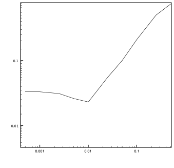
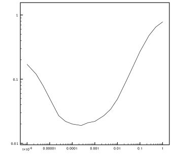
Figure 1: Study of the global relative $L^{2}$-error against penalty parameters $\gamma_{V}$ and $\gamma_{W}$ for the methods using (5.4) (left) and (5.3) (right).

5.2 Convergence studies

We know that the problem becomes increasingly ill-posed as $n$ becomes large, but that the stabilities given by (1.3) and (1.4), (1.5) hold independently of $n$. We performed computations varying $n$ from $1$ to $5$ on a series of unstructured meshes with approximate meshsizes in the set,

$$\{0.1,\,0.05,\,0.025,\,0.0125,\,0.008333\}.$$

Herein we only present the results of the computations for odd $n$. The results are given in Figures 2 - 4. We have studied the relative $L^{2}$-norms for the four different values of $\zeta$ given in (5.7). Each value of $\zeta$ is represented by a different symbol according to $\zeta=1$, symbol: $\circ$; $\zeta=1/2$, symbol: $\square$; $\zeta=1/4$, symbol: $\diamond$; $\zeta=1/8$, symbol: $\bigtriangleup$. Filled symbols are used for graphs representing the $H^{1}$-error. As we increase the value of $n$ the $H^{1}$-norm of the exact solution, denoted $E$, increases and is given in the captions of the figures. We see that the error level increases with increasing $E$. For the lower values $n=1$ and $n=3$ we observe typically $O(h^{\frac{3}{2}})$ convergence in the $L^{2}$-norm for all quantities. The global error takes relatively smaller values for higher $n$ compared to the local error quantities as an effect of the normalization. For $n=5$ the method using (5.4) appears to have approximately $O(h)$ convergence. The same global convergence behavior is observed for the method using (5.3), but in this case the convergence is uneven although the errors are smaller than for (5.4). The observed superconvergence compared to the theoretical results can be attributed to the fact that in these computations, the error in the $H^{1}$-norm also decreased, making the constants $C(E)$ and $C_{1}(E)$ of equations (1.4), (1.5) decrease as well. We illustrate this for the case $n=5$ in Figure 5.

Observe that (1.4) and (1.5) are valid also in the limit of $n\rightarrow\infty$ and it appears that the logarithmic continuous dependence is not dominating on the relatively low values of $n$ and large values of $h$, considered herein. For larger values of $n$ the $H^{2}$-norm of the exact solution becomes so large that the computations on the meshes considered are not in the asymptotic range. For $n=7$ the linear decrease predicted in Proposition 4.1, independently of the stability of the problem, was not observed.

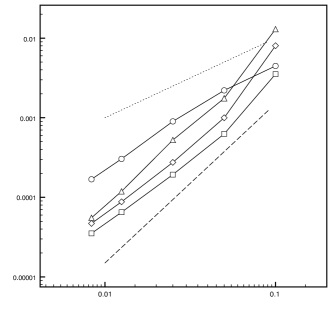
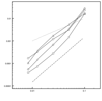
Figure 2: Relative $L^{2}$-error against mesh-size, $n=1$ in (5.5) and $E=1.68$, using the stabilizations (5.4) (left) and (5.3) (right). Reference curves: $y=0.1x$ (dotted) and $y=0.15x^{2}$ (dashed)

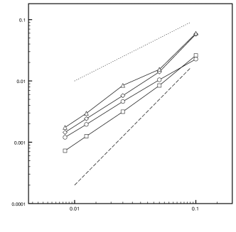
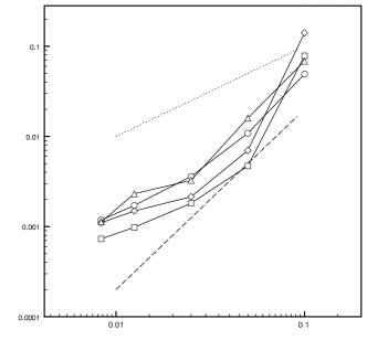
Figure 3: Relative $L^{2}$-error against mesh-size, $n=3$ in (5.5) and $E=7.27$, using the stabilizations (5.4) (left) and (5.3) (right). Reference curves: $y=x$ (dotted) and $y=2x^{2}$ (dashed)

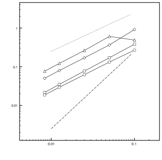
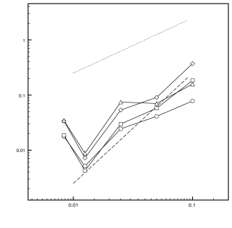
Figure 4: Relative $L^{2}$-error against mesh-size, $n=5$ in (5.5) and $E=41.6$, using the stabilizations (5.4) (left) and (5.3) (right). Reference curves: $y=25x$ (dotted) and $y=25x^{2}$ (dashed)

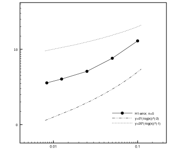
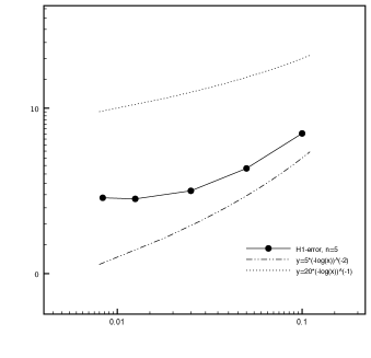
Figure 5: Absolute $H^{1}$-error against mesh-size, $n=5$ in (5.5) and $E=41.6$, using the stabilizations (5.4) (left) and (5.3) (right). Reference curves: $y=-20log(x)^{-1}$ (dotted) and $y=-5log(x)^{-2}$ (dash-dot)

6 Concluding remarks

We have proposed a nonconforming stabilized finite element method for the approximation of elliptic Cauchy problems. Two different stabilization operators were studied. The operator (5.3) was shown to give better control over perturbations in data, whereas (5.4) is adjoint consistent, possibly performing better for the computation of certain linear functionals. We proved a posteriori and a priori error estimates for both approaches under the assumption of continuous dependence. Numerically both methods were shown to have similar performance, but the method using (5.3) was sensitive to over-stabilization on high resultion computations for high frequency solutions. This method also needed separate tuning of the parameters $\gamma_{V}$ and $\gamma_{W}$, whereas they could be chosen equal for the method using (5.4).

References

• [1] Y. Achdou, C. Bernardi, and F. Coquel, A priori and a posteriori analysis of finite volume discretizations of Darcy’s equations, Numer. Math. 96 (2003), no. 1, 17–42. MR 2018789 (2005d:65179)
• [2] G. Alessandrini, L. Rondi, E. Rosset, and S. Vessella, The stability for the Cauchy problem for elliptic equations, Inverse Problems 25 (2009), no. 12, 123004, 47. MR 2565570 (2010k:35517)
• [3] S. Andrieux, T. N. Baranger, and A. Ben Abda, Solving Cauchy problems by minimizing an energy-like functional, Inverse Problems 22 (2006), no. 1, 115–133. MR 2194187 (2007b:35084)
• [4] M. Azaïez, F. Ben Belgacem, and H. El Fekih, On Cauchy’s problem. II. Completion, regularization and approximation, Inverse Problems 22 (2006), no. 4, 1307–1336. MR 2249467 (2008b:35043)
• [5] F. Ben Belgacem, Why is the Cauchy problem severely ill-posed?, Inverse Problems 23 (2007), no. 2, 823–836. MR 2309677 (2008c:35331)
• [6] L. Bourgeois, A mixed formulation of quasi-reversibility to solve the Cauchy problem for Laplace’s equation, Inverse Problems 21 (2005), no. 3, 1087–1104. MR 2146823 (2006b:35334)
• [7]  , Convergence rates for the quasi-reversibility method to solve the Cauchy problem for Laplace’s equation, Inverse Problems 22 (2006), no. 2, 413–430. MR 2216406 (2007d:35277)
• [8] E. Burman, Stabilized finite element methods for nonsymmetric, noncoercive, and ill-posed problems. Part I: Elliptic equations, SIAM J. Sci. Comput. 35 (2013), no. 6, A2752–A2780. MR 3134434
• [9]  , Error estimates for stabilized finite element methods applied to ill-posed problems, Tech. report, arXiv, 2014.
• [10] E. Burman and P. Hansbo, Stabilized Crouzeix-Raviart element for the Darcy-Stokes problem, Numer. Methods Partial Differential Equations 21 (2005), no. 5, 986–997. MR 2154230 (2006i:65190)
• [11] A. Chakib and A. Nachaoui, Convergence analysis for finite element approximation to an inverse Cauchy problem, Inverse Problems 22 (2006), no. 4, 1191–1206. MR 2249460 (2007h:49040)
• [12] M. Crouzeix and P.-A. Raviart, Conforming and nonconforming finite element methods for solving the stationary Stokes equations. I, Rev. Française Automat. Informat. Recherche Opérationnelle Sér. Rouge 7 (1973), no. R-3, 33–75. MR 0343661 (49 #8401)
• [13] J. Dardé, A. Hannukainen, and N. Hyvönen, An $H_{\sf{div}}$-based mixed quasi-reversibility method for solving elliptic Cauchy problems, SIAM J. Numer. Anal. 51 (2013), no. 4, 2123–2148. MR 3079321
• [14] R. Eymard, T. Gallouët, and R. Herbin, Error estimate for approximate solutions of a nonlinear convection-diffusion problem, Adv. Differential Equations 7 (2002), no. 4, 419–440. MR 1869118 (2002h:35156)
• [15] R. S. Falk and P. B. Monk, Logarithmic convexity for discrete harmonic functions and the approximation of the Cauchy problem for Poisson’s equation, Math. Comp. 47 (1986), no. 175, 135–149. MR 842126 (87j:65109)
• [16] J. Hadamard, Sur les problèmes aux derivées partielles et leur signification physique., Bull. Univ. Princeton (1902).
• [17] H. Han, L. Ling, and T. Takeuchi, An energy regularization for Cauchy problems of Laplace equation in annulus domain, Commun. Comput. Phys. 9 (2011), no. 4, 878–896. MR 2734356
• [18] W. Han, J. Huang, K. Kazmi, and Y. Chen, A numerical method for a Cauchy problem for elliptic partial differential equations, Inverse Problems 23 (2007), no. 6, 2401–2415. MR 2441010 (2009f:65138)
• [19] P. Hansbo and M. G. Larson, Discontinuous Galerkin methods for incompressible and nearly incompressible elasticity by Nitsche’s method, Comput. Methods Appl. Mech. Engrg. 191 (2002), no. 17-18, 1895–1908. MR 1886000 (2003j:74057)
• [20]  , Discontinuous Galerkin and the Crouzeix-Raviart element: application to elasticity, M2AN Math. Model. Numer. Anal. 37 (2003), no. 1, 63–72. MR 1972650 (2004b:65184)
• [21] F. Hecht, New development in freefem++, J. Numer. Math. 20 (2012), no. 3-4, 251–265. MR 3043640
• [22] O. A. Karakashian and F. Pascal, A posteriori error estimates for a discontinuous Galerkin approximation of second-order elliptic problems, SIAM J. Numer. Anal. 41 (2003), no. 6, 2374–2399 (electronic). MR 2034620 (2005d:65192)
• [23] R. Lattès and J.-L. Lions, The method of quasi-reversibility. Applications to partial differential equations, Translated from the French edition and edited by Richard Bellman. Modern Analytic and Computational Methods in Science and Mathematics, No. 18, American Elsevier Publishing Co., Inc., New York, 1969. MR 0243746 (39 #5067)
• [24] W. Lucht, A finite element method for an ill-posed problem, Appl. Numer. Math. 18 (1995), no. 1-3, 253–266, Seventh Conference on the Numerical Treatment of Differential Equations (Halle, 1994). MR 1357921 (96f:65154)
• [25] H.-J. Reinhardt, H. Han, and Dinh Nho Hào, Stability and regularization of a discrete approximation to the Cauchy problem for Laplace’s equation, SIAM J. Numer. Anal. 36 (1999), no. 3, 890–905. MR 1681021 (2000a:65166)
• [26] A. N. Tikhonov and V. Y. Arsenin, Solutions of ill-posed problems, V. H. Winston & Sons, Washington, D.C.: John Wiley & Sons, New York-Toronto, Ont.-London, 1977, Translated from the Russian, Preface by translation editor Fritz John, Scripta Series in Mathematics. MR 0455365 (56 #13604)