STREGA: STRucture and Evolution of the GAlaxy. I. Survey Overview and First Results

Abstract

STREGA (STRucture and Evolution of the GAlaxy) is a Guaranteed Time survey being performed at the VST (the ESO VLT Survey Telescope) to map about 150 square degrees in the Galactic halo, in order to constrain the mechanisms of galactic formation and evolution. The survey is built as a five-year project, organized in two parts: a core program to explore the surrounding regions of selected stellar systems and a second complementary part to map the southern portion of the Fornax orbit and extend the observations of the core program. The adopted stellar tracers are mainly variable stars (RR Lyraes and Long Period Variables) and Main Sequence Turn-off stars for which observations in the $g$,$r$,$i$ bands are obtained. We present an overview of the survey and some preliminary results for three observing runs that have been completed. For the region centered on $\omega$ Cen (37 deg²), covering about three tidal radii, we also discuss the detected stellar density radial profile and angular distribution, leading to the identification of extratidal cluster stars. We also conclude that the cluster tidal radius is about 1.2 deg, in agreement with values in the literature based on the Wilson model.

1 Introduction

The formation and evolution of galaxies and their relation with the environment, from the scale of the Local Group to superclusters, has been a major field of astronomical research in the past decade. The first laboratory for studying mechanisms of galactic formation and evolution and their dependence on the surrounding environment is represented by the Milky Way (MW) and its satellite galaxies. For nearby systems, indeed, accurate photometry can be obtained for individual members of the various stellar populations. Several investigations have shown that the outer regions of the Galactic halo do not have a smooth distribution of stars but appear quite “clumpy” (see e.g. Vivas & Zinn, 2003; Newberg et al., 2003; Bell et al., 2010; Drake et al., 2013; Zinn et al., 2014), in agreement with theoretical models of the hierarchical formation of structures based on a Cold Dark Matter cosmology (Navarro et al., 1997; Mateo, 1998; Da Costa, 1999; Benson et al., 2002; Tumlinson, 2010; Wang et al., 2013). Among the most spectacular examples of Galactic halo substructures we cite:

• The Sagittarius dwarf spheroidal galaxy currently merging with the MW halo and its associated stream (see e.g. Ibata et al., 1994; Bellazzini et al., 2006; Deg & Widrow, 2013, and references therein);

• the stellar over-density in the Canis Major region whose origin is still a matter of debate (Martin et al., 2004; Momany et al., 2006; Mateu et al., 2009; López-Corredoira et al., 2007; Saviane et al., 2011, and references therein);

• the presence of peculiar Galactic Globular Clusters (GGCs) with observed tidal tails or suspected halos (see e.g. Fellhauer et al., 2007; Odenkirchen et al., 2001, 2009; Olszewski et al., 2009; Chun et al., 2010; Walker et al., 2011; Lane et al., 2012a, b; Majewski et al., 2012, and references therein);

• the discovery of several ultra-faint companions of the MW from analysis of the Sloan Digital Sky Survey (SDSS) data (Belokurov et al., 2006, 2007; Musella et al., 2009, 2012; Moretti et al., 2009; Clementini et al., 2012; Dall’Ora et al., 2006, 2012; Garofalo et al., 2013, and references therein). Note that similar substructures have been also found in the M31 halo (e.g. Gilbert et al., 2009; Richardson et al., 2008; Clementini et al., 2011).

Dating back to Lynden-Bell (1976, 1982); Demers & Kunkel (1979); Lynden-Bell & Lynden-Bell (1995), it was suggested that the dwarf spheroidal satellites (dSphs) of the Galaxy and a number of its globular clusters (GCs) are distributed along planar alignments reflecting distinct orbital planes and usually interpreted as the result of the disruption of larger galaxies. The location of these systems has recently been claimed to define a vast polar structure (VPOS; Pawlowski et al., 2012; Pawlowski & Kroupa, 2013) and a similar plane has been detected with very high significance in M31 (Conn et al., 2013; Ibata et al., 2013). A very interesting example of these alignments is the so called Fornax stream that should include both dSphs (Fornax, Leo I, Leo II, Sculptor and possibly Sextans and Phoenix ) and GCs (Pal 3, Pal 4 and Pal 12), as also discussed in Majewski (1994). Even if the measurements of the absolute proper motion of Fornax (Dinescu et al., 2004), together with the shell structures identified by Coleman et al. (2004), already provided some circumstantial evidence, accurate observations of large fractions of the Fornax orbit are still lacking. According to recent N-body simulations (see e.g. Mayer et al., 2002; Hayashi et al., 2003; Read et al., 2006; Madau et al., 2008; Mayer, 2011, and references therein), in the interaction of small satellites (e.g. dSphs and GCs) with the MW, tidally stripped material should form elongated tidal tails and spherical shells extending many scale radii beyond the tidal radius.

Evidence of tidal tails has been found in connection with several GCs, for example Pal 14 and NGC1851 (see e.g. Sollima et al., 2011, 2012, and references therein), M15, M30, M53, NGC5053, NGC5466 (Chun et al., 2010) Pal 5 (Odenkirchen et al., 2001) and also NGC5139 (see e.g. Leon et al., 2000; Majewski et al., 2012, $\omega$ Cen). This last cluster is of particular interest. It has been claimed to be the remnant of a tidally disrupted galaxy because of: i) its internal chemical and age distribution with the presence of multiple stellar populations; ii) its similarity for mass and chemistry to M54, the GC associated with the core of the disrupting Sagittarius galaxy (see discussion in Majewski et al., 2012) and iii) its unusual low-inclination, retrograde orbit. Even if simulations of the tidal disruption of $\omega$ Cen suggested the presence of stripped cluster stars in the Solar Neighborhood, the observation of these extratidal stars only produced preliminary results (see e.g. Leon et al., 2000) that were later found to be biased by substantial foreground differential reddening problems (Law et al., 2003). Subsequently Da Costa & Coleman (2008) estimated that only a very small fraction of cluster members in the Red Giant Branch (RGB) phase were actually stripped stars. Majewski et al. (2012) has recently reported the detection of “tidal debris” consistent with that modeled for $\omega$ Cen.

Another interesting GC hosting multiple stellar populations is NGC6752 (see e.g. Carretta, 2013; Milone et al., 2013, and references therein). Even if the proper motion of this cluster has been extensively investigated (see e.g. Dinescu et al., 1999; Drukier et al., 2003; Zloczewski et al., 2012), a systematic investigation of extra-tidal stellar populations around this cluster is lacking in the literature.

The outer-halo sparse GC Pal 12 is probably younger than the bulk of GGCs (see e.g. Rosenberg et al., 1998) and has been suggested to have been tidally captured from the Sgr dSph galaxy by the Milky Way (Irwin, 1999). A tidal stream of debris from the Sgr dSph galaxy towards the Galactic halo has been observed both by the Two Micron All Sky Survey (2MASS Majewski et al., 2003) and by the SDSS (Ivezic et al., 2004) and various authors have shown that Pal 12 is embedded in this stream (see e.g. Bellazzini et al., 2003; Martínez-Delgado et al., 2002; Cohen, 2004).

Finally, it is worth noting that signatures of extratidal stellar populations have been detected around a number of nearby dSphs (e.g. Irwin & Hatzidimitriou, 1995; Majewski et al., 2000; Mateo et al., 2008; Pawlowski et al., 2012, and references therein). A typical example is the Carina galaxy for which several authors have investigated the presence of tidal tails (Kuhn et al., 1996; Monelli et al., 2004; Muñoz et al., 2006).

In this context, the STRucture and Evolution of the GAlaxy (STREGA) survey plans to use the VLT Survey Telescope (VST) to investigate Galactic halo formation mechanisms through the two following observing strategies: i) tracing tidal tails and halos around stellar clusters and galaxies; ii) mapping extended regions of the southern portion of the Fornax orbit to trace the Fornax Stream. In addition, our strategy can in principle allow us to identify unknown very faint stellar systems by using well established techniques developed in the context of the SDSS (e.g. Belokurov et al., 2006).

In this paper, we describe the instrument, namely the VST and OmegaGAM (Section 2) and the STREGA survey (Section 3). In Section 4, we present the observations for the three completed runs, covering the GGCs $\omega$ Cen, NGC6752 and Pal 12, whereas the procedures used for the data reductions are discussed in Section 5. The adopted tools and some preliminary results for the fields around NGC6752 and $\omega$ Cen are shown in Section 6. The Conclusions and some final remarks close the paper.

2 Observing with VST

The VST is a 2.6-m wide-field optical telescope built by INAF-Osservatorio Astronomico di Capodimonte, Naples (Italy) and located at Cerro Paranal (Chile) on the VLT platform. It is characterized by an alt-azimuth mount with a f/5.5 modified Ritchey-Chré tien optics (see Capaccioli & Schipani, 2011, for further details). The telescope is equipped with OmegaCAM (Kuijken, 2011), a camera with a field of view of $1^{\circ}$ x $1^{\circ}$, built by a consortium of European institutes, featuring a 32-CCD, 16k x 16k detector mosaic, with a pixel size of 0.21 arcsec. The filter system includes the USNO $u^{\prime}g^{\prime}r^{\prime}i^{\prime}z^{\prime}$ bands, the Johnson $B$ and $V$ filters, and a number of narrow-band filters mosaics such as segmented $H\alpha$ and $vS$. It is important to note that even if the VST filter system is based on the USNO $u^{\prime}g^{\prime}r^{\prime}i^{\prime}z^{\prime}$ system (Smith et al., 2002), slightly different from SDSS $ugriz$ (for details, see the “Photometry White Paper” by Gunn et al. 2001), we calibrate our data to the “natural” SDSS system. For this reason, in the following, we use the $ugriz$ notation. Finally, we remind the reader that the OmegaCAM calibration plan ensures for the VST data a photometric and astrometric calibration at 0.05 mag and 0.1 arcsec rms precision levels, respectively.

3 The survey STREGA@VST

STREGA@VST (P.I.: M. Marconi/I. Musella, see also Marconi et al., 2014) was conceived as a five-year survey, organized in two parts: a core program and a second part. In the core program we are exploring the outskirts of selected dSphs and GCs up to at least 2–3 tidal radii in several directions to distinguish between tidal tails and halos. These systems are located either along the Fornax orbit or are of particular interest for the interaction mechanism with the Galactic halo: Fornax and Sculptor (38 fields), Phoenix (3 fields), Sextans (13 fields), Pal 3 (3 fields), Pal 12 (1 field), $\omega$ Cen and NGC6752 (33 and 32 fields around each GC, respectively). In Fig. 1 we show the location of the core program targets (red symbols).

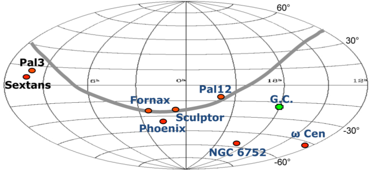
Figure 1: The selected STREGA core program targets (red symbols) in equatorial coordinates, compared with the location of the Galactic Center (green symbol) and Fornax orbit according to Dinescu et al. (2004).

The second part will cover strips of adjacent fields distributed transverse to Fornax orbit and will extend the observations of the most interesting systems explored in the core program to larger radial distances.

To investigate the mechanisms of the formation and evolution of the Galactic halo, the STREGA survey mainly relies on variable stars (RR Lyrae stars and Long Period Variables) and Main Sequence Turn-off (MSTO) stars (see e.g. Cignoni et al., 2007). The former are easily detectable thanks to their brightness and characteristic light curves (see e.g. Vivas & Zinn, 2006; Mateu et al., 2009; Prior et al., 2009). The latter are about 3.5 mag fainter than RR Lyrae stars but at least 100 times more abundant. Moreover, the accurate sampling of the light curves of the identified RR Lyrae stars is used to characterize their stellar properties providing clues on the Galactic halo star formation history (Clementini et al., 2011, and references therein). The multi-purpose nature of the STREGA survey aims at a few additional objectives including the sampling of the brightest field single white dwarfs (WDs) and interacting binaries (IBs), most being accreting compact objects with low-mass donor companions. In this respect our survey complements the VST Photometric H$\alpha$ Survey of the Southern Galactic Plane (VPHAS+ Drew et al., 2014) that will map the disk population of IBs. As for the single WDs, our relatively deep fields at different Galactic latitudes will allow us to study the poorly known WD parameter space in the various Galactic populations, including thin disk, thick disk and spheroid populations, complementing the recent statistical studies based on much larger, but shallower, WD samples from the SDSS and SuperCOSMOS surveys (De Gennaro et al., 2008; Rowell & Hambly, 2011). We will use different filter strategies, with the narrow $vS$ filter to sample hot WDs and the broad SDSS filters for cool/ultracool WDs. Similar to the case with IBs and especially for the halo candidates, multi-epoch observations and follow-up IR photometry and/or spectroscopy will allow us to confirm the true nature of these objects.

4 The Observations

Observations for the VST INAF GTO started at the end of 2011 and proposals have been approved for Periods from 88 to 93 (088.D-4015, 089.D-0706, 090.D-0168, 091.D-0623, 092.D-0732, 093.D-0170). However, also due to technical and scheduling problems, only a minor part of the observations for the STREGA core program have been gathered so far (see Table 1). In particular the only completed patches are the fields around $\omega$ Cen (observed in the ESO Period 88), NGC6752 (Period 89) and Pal 12 (Period 91). Additional data for the central region of $\omega$ Cen (4 fields) were observed subsequently to P88 in visitor mode (March 2013).

Table 1: Distribution of the service mode observations. The first column indicates the ESO Period. The second and third columns give the requested and observed time, respectively. The last column reports the ESO OB class percentage.

ESO Period	Requested [h]	Observed [h]	% OB Class A,B,D
88	28	3.8	26,67,7
89	38.4	3.8	22,76,2
90	47.9	9.4	50,39,11
91	39.6	8.9	38,37,25
92	18.0	11.7	59,37,4
93	33.0	OPEN	—

Due to the relatively short distance modulus of the globular clusters $\omega$ Cen ($\approx$13.7 mag; Del Principe et al., 2006), NGC6752 ($\approx$13.2 mag; Milone et al., 2013) and Pal 12 ($\approx$16.5 mag; Rosenberg et al., 1998), the exposure times to reach the RR Lyrae magnitude level in these systems are of the order of a very few seconds, dramatically shorter than telescope overheads. In these cases variability should be investigated with suitable follow-up observations on the most interesting fields. On the other hand, thanks to its wide field of view and high resolution, VST is the ideal instrument to perform a map of extra-tidal stellar populations or of the extended halo around these systems, through observations down to the MSTO and fainter MS stars. Therefore, we planned to observe the selected fields to deeper magnitude limits (exposure times of tens of seconds) to build color-magnitude and color-color diagrams. The fields observed for $\omega$ Cen and NGC6752 were selected to uniformly map the outskirts of the cluster up to 3 tidal radii, by adopting the Survey Area Definition Tool (SADT; Arnaboldi et al, 2008). In Figs. 2 and 3, we show the obtained sky field distributions. For Pal 12, we observed a single field centered on the cluster, covering about 2 tidal radii.

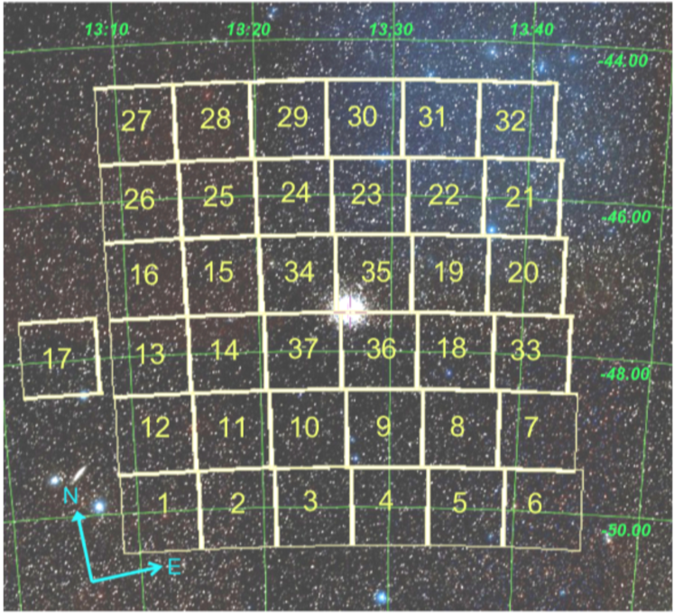
Figure 2: Observed fields by OMEGACAM@VST around the Globular Cluster $\omega$ Cen, in equatorial coordinates.

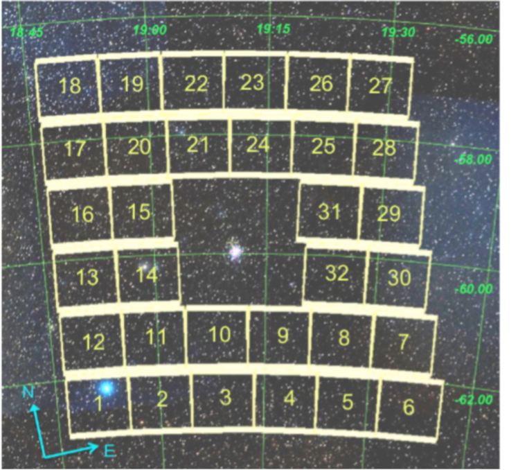
Figure 3: As in Fig. 2 but for NGC6752.

5 Data reduction

The data reduction has made use of the newly developed VST–Tube imaging pipeline (Grado et al., 2012), specifically conceived for the data coming from the VST telescope but adaptable to other existing or future single or multi-CCD cameras. The data processing includes removal of instrumental signatures, namely overscan, bias and flatfleld correction, CCDs gain harmonization and illumination correction. Relative and absolute astrometric and photometric calibration were applied to the individual exposures. In detail, the bias level is measured from the median value of a suitable portion of the overscan region, then the bias map (masterbias) is derived after a sigma-clipped averaging of the bias frames. The flat-field correction (masterflat) is a combination of the average twilight flats (from a number of twilight flats), that correct for pixel-to-pixel sensitivity variation, and a super skyflat, obtained with a combination of science images, that accounts for the low spatial frequency gain variations. In order to set all the mosaic chips to the same zeropoint, a gain harmonization procedure was required. The procedure measures the relative gain coefficients that give the same background signal in adjacent CCDs. For the VST data it was necessary to apply an additional correction for the scattered light. This is a common problem for wide-field imagers where telescope and instrument baffling can be an issue. The off-axis uncontrolled redistribution of light paths gives an additive component to the background, with a peak in the central area, so that the flat field will not be an accurate estimate of the spatial detector response. Indeed, if this effect is not corrected, the image background will appear perfectly flat, but the photometric response will be position dependent (Andersen et al., 1995). This error in the determination of the flat-field can be mitigated through the determination and application of the so called illumination correction (IC) map. The IC map was determined by comparing the magnitudes of equatorial photometric standard fields stars with extracted catalogs from the SDSS DR8. The magnitude residuals as a function of the position were fitted using a generalized adaptive method (GAM) in order to obtain a 2D map used to correct the science images during the pre-reduction stage. The GAM allows us to obtain a good surface also in case the field of view is not uniformly sampled by the standard stars. The absolute photometric calibration (see Table 2) was computed comparing the aperture magnitude (Bertin & Arnouts, 1996) of photometric standard-field stars with reference catalogs from SDSS DR8. A simultaneous fit of the zero-point and color term was performed using Photcal (Radovich et al., 2004), while the extinction coefficients were those (mean values) extracted from the extinction curve provided by the ESO calibration team. Relative photometric corrections, accounting for transparency variations among exposures, as well as absolute and relative astrometric calibration, were obtained using SCAMP (Bertin, 2006). Resampling and stacking of the individual exposures was obtained using SWARP (Bertin, 2002).

Table 2: Calibration Log. The table reports the observed target, the adopted filters, the night used for the absolute photometric calibration and the corresponding zero point, color term and extinction coefficient

Target	Filter	night	Zero-Point (mag)	Color term	Ext. coeff. (mag)
$\omega$ Cen	g	2012-03-21	24.650 $\pm$ 0.010	0.024 $\pm$ 0.009 $(g-i)$	0.110
$\omega$ Cen	r	2012-04-02	24.502 $\pm$ 0.008	0.043 $\pm$ 0.020 $(r-i)$	0.030
$\omega$ Cen	i	2012-03-04	24.013 $\pm$ 0.011	-0.001 $\pm$ 0.008 $(g-i)$	0.010
$\omega$ Cen	g	2013-03-15/19	24.699 $\pm$ 0.006	0.024 $\pm$ 0.006 $(g-i)$	0.180
$\omega$ Cen	r	2013-03-15/19	24.601 $\pm$ 0.005	0.049 $\pm$ 0.013 $(r-i)$	0.100
$\omega$ Cen	i	2013-03-15/19	24.119 $\pm$ 0.006	-0.002 $\pm$ 0.005 $(g-i)$	0.043
NGC6752	g	2012-05-05	24.799 $\pm$ 0.010	0.017 $\pm$ 0.010 $(g-i)$	0.180
NGC6752	r	2012-05-01	24.598 $\pm$ 0.006	0.054 $\pm$ 0.016 $(r-i)$	0.100
NGC6752	i	2012-05-08	24.136 $\pm$ 0.006	-0.002 $\pm$ 0.016 $(g-i)$	0.043
PAL 12	g	2013-07-01	24.809 $\pm$ 0.008	0.033 $\pm$ 0.007 $(g-i)$	0.180
PAL 12	r	2013-07-01	24.633 $\pm$ 0.006	0.053 $\pm$ 0.017 $(r-i)$	0.100
PAL 12	i	2013-07-01	24.113$\pm$ 0.007	-0.002 $\pm$ 0.006 $(g-i)$	0.043

The stellar photometry in the crowded stellar clusters must be performed by using the Point Spread Function (PSF) fitting method (e.g. Stetson, 1987), while for uncrowded fields, to obtain accurate magnitudes, we could also use aperture photometry. In practice, for crowded fields we use DAOPHOT/ALLSTAR (Stetson, 1987), one of the most used packages to obtain very accurate PSF magnitudes, and for measuring aperture photometry we adopt SExtractor (Bertin & Arnouts, 1996). The latter is currently adopted for extragalactic studies, but it is particularly suited for wide-field images, being fast, fully automatisable and able to give accurate results for stellar photometry in not severely crowded fields. For each source, SExtractor provides several different parameters to characterize the brightness and the shape. The proper aperture magnitude for stellar objects is the so called MAG_APER parameter. Indeed it gives a measure of the total magnitude within a circular aperture with a fixed user-supplied radius. In our analysis, we adopt an aperture radius of 20 pixels (correposnding to $\sim 5\times FWHM$ for typical seeing) that encloses more than 99.99$\%$ of the light of a selected, isolated and good number of stars among the brightest ones. Moreover, to check the consistency of the photometry we compared the SExtractor with the DAOPHOT/ALLSTAR measurements, for selected images.

To clean the catalogs obtained by DAOPHOT/ALLSTAR of objects with noisy photometry, we selected the objects with $\chi<1.6$ and $-0.2<$Sharp$<0.2$ .

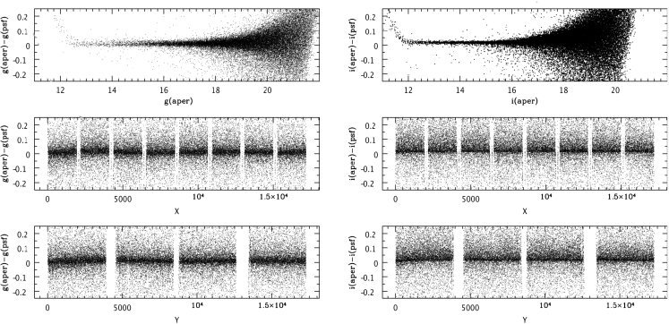
Figure 4: Residual between $g$ (left panel) and $i$ (right panel) magnitudes estimated by SExtractor and the PSF ones obtained with DAOPHOT/ALLSTAR (accounting for the different instrumental magnitude zero-point) as a function of the aperture magnitude and of the position on the frame, in the case of the selected reference field ($l$,$b=$306.2,12.78; Field 1 around $\omega$ Cen).

Fig. 4 shows the residuals of the SExtractor and DAOPHOT photometry, as a function of the magnitude and the field position in the case of a selected pointing ($l$,$b=$306.2,12.78; Field #1 around $\omega$ Cen), both in $g$ (left panel) and $i$ (right panel) bands. We note that SExtractor aperture photometry, in the case of uncrowded fields, is comparable with the more time-consuming DAOPHOT PSF photometry, at least in the magnitude range 12.5–21 mag, with a maximum discrepancy of 0.2 mag. At brighter magnitudes the deviation, more evident in the $i$ band, is due to nonlinearity of the CCDs.

Through this comparison between the aperture SExtractor photometry and that obtained by DAOPHOT/ALLSTAR we also verified that, in the case of the SExtractor catalog, the contamination by non-stellar objects affects a magnitude range fainter than the completeness limit (see Sect. 7) and therefore out of interest for our purposes.

The photometry on the fields including the central part of $\omega$ Cen (#34, #35, #36 and #37) and on the field centered on Pal 12 was performed only using the DAOPHOT/ALLSTAR packages. The calibration of the four central pointings on $\omega$ Cen, observed on a non-photometric night, was checked with the deep and accurate $UBVRI$ photometry published in Castellani et al. (2007), transformed to the $ugriz$ photometric system by adopting the equations computed for the Population II stars, based on the transformations devised by Jordi et al. (2006). For each field and for each filter, the mean offset between our measured magnitudes and the transformed magnitudes was applied as a zero-point correction. The four corrected catalogs were merged into a single catalog, which is used for the subsequent analysis. Similarly for the field centered on Pal 12, we checked the photometric calibration by comparison with independent very accurate $BVI$ photometry by one of us (P.B. Stetson, hereinafter PBS, unpublished). In the case of NGC6752, waiting for the VST observations of the central fields, we performed a qualitative comparison of the color-magnitude diagrams for the external fields againts the central one, the latter obtained from unpublished photometry by PBS, finding a satisfactory agreement (see the following section).

6 Color-Magnitude Diagrams

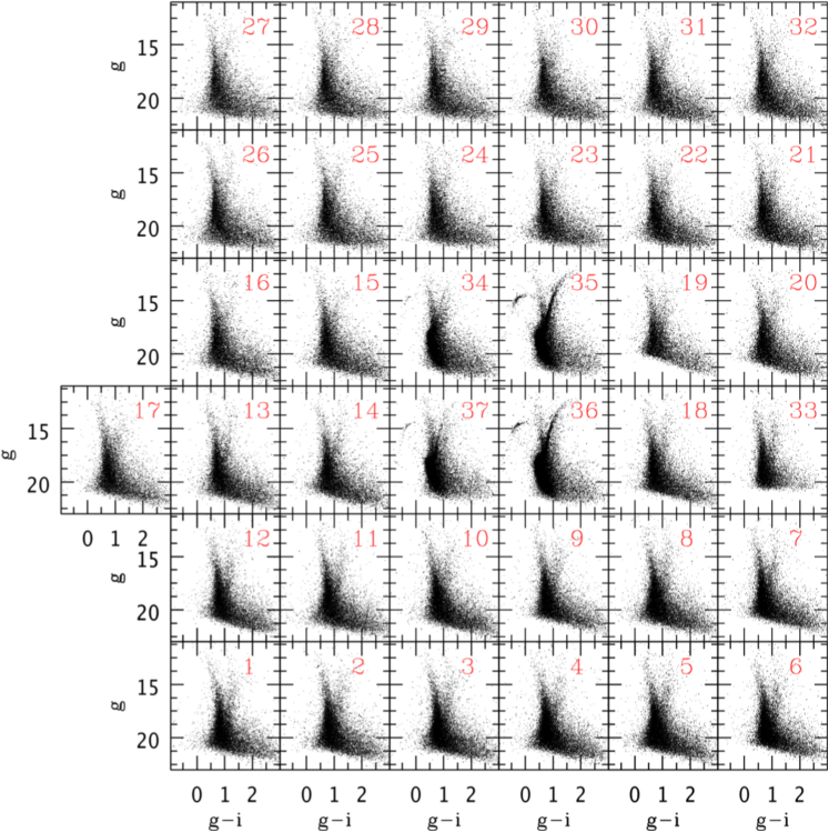
Figure 5: CMDs of the stars in the 37 fields on and around $\omega$ Cen. For orientation of the fields, see Fig. 2

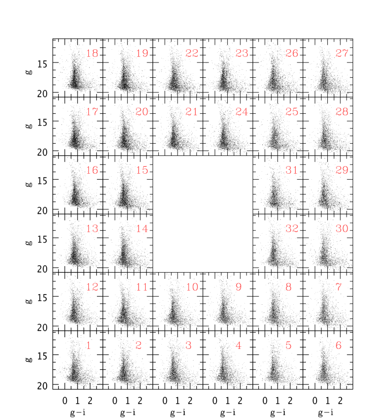
Figure 6: CMDs of the stars observed in the 32 fields around NGC6752. For orientation of the fields, see Fig. 3.

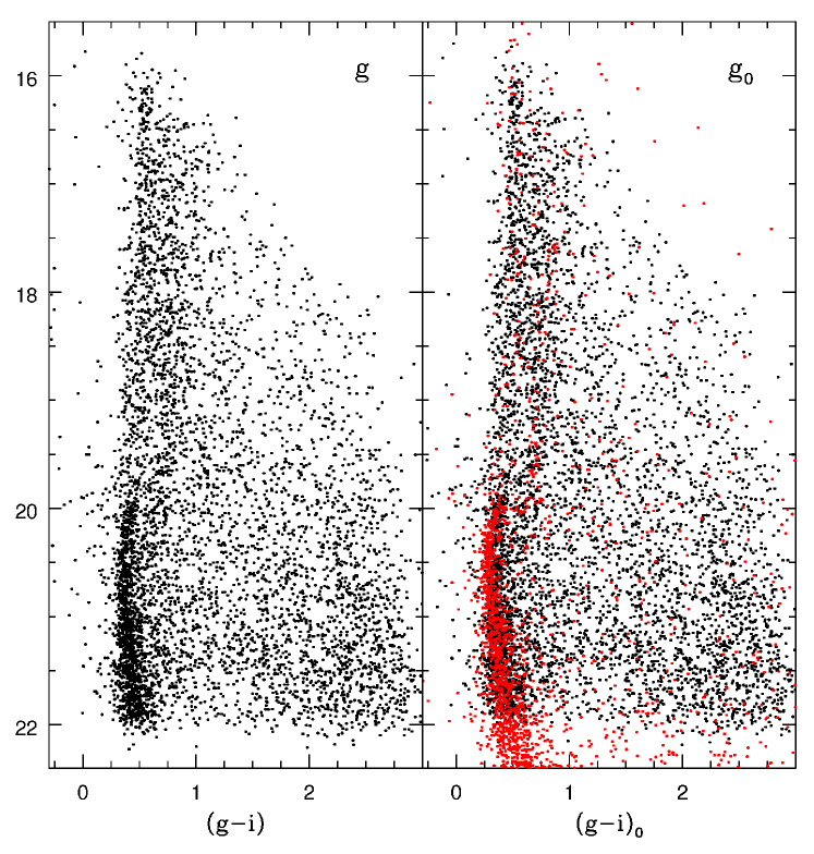
Figure 7: CMD for the field centered on Pal 12, before (left panel) and after (right panel) reddening correction. The reddening correction is negligible, but in the right panel, we also show the cluster photometry obtained by PBS (red symbols, see text for details).

Figures 5, 6 and the left panel of 7 show the color-magnitude diagrams (CMDs) for $\omega$ Cen, NGC6752 and Pal 12, in all the investigated fields, obtained by combining the two independently selected $g$-band and $i$-band catalogs and adopting a 0.25 arcsec matching radius.

To investigate the signature of over-densities associated with various CMD features, it is important to take into account the differential reddening contribution as well as the contamination from the various Galactic components.

6.1 The differential reddening issue

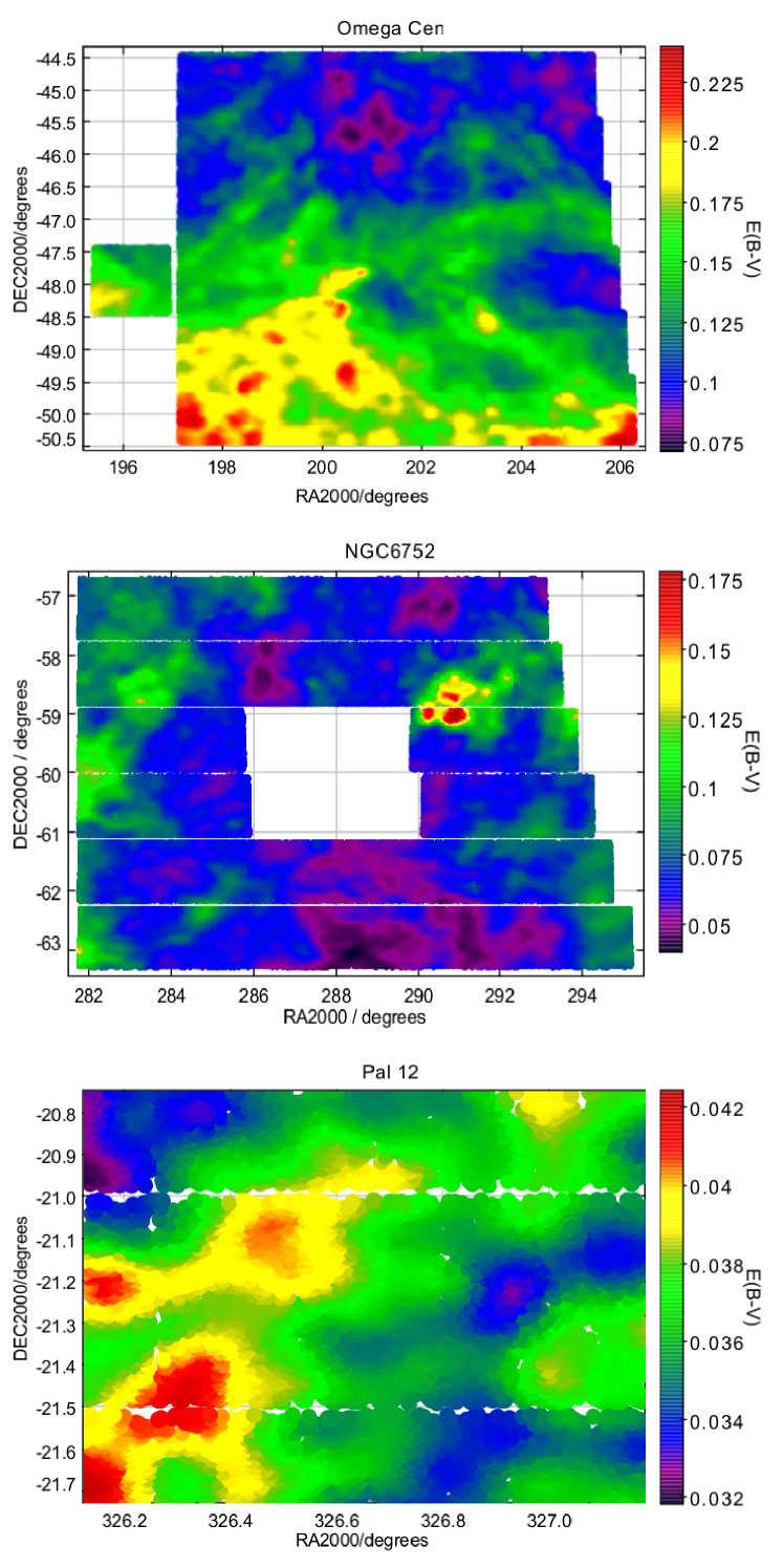
Figure 8: The extinction maps of Schlegel et al. (1998) recalibrated by Schlafly & Finkbeiner (2011) for the observed fields around $\omega$ Cen, NGC6752 and Pal 12.

In Fig. 8 we report the extinction maps of Schlegel et al. (1998) recalibrated by Schlafly & Finkbeiner (2011) for the observed fields. Significant differential reddening appears only around $\omega$ Cen (note the differences among the color scales), due to the closeness of the lowest fields to the Galactic disk. For NGC6752 and Pal 12, the reddening is rather uniform apart from a small region around NGC6752 close to the Galactic disk.

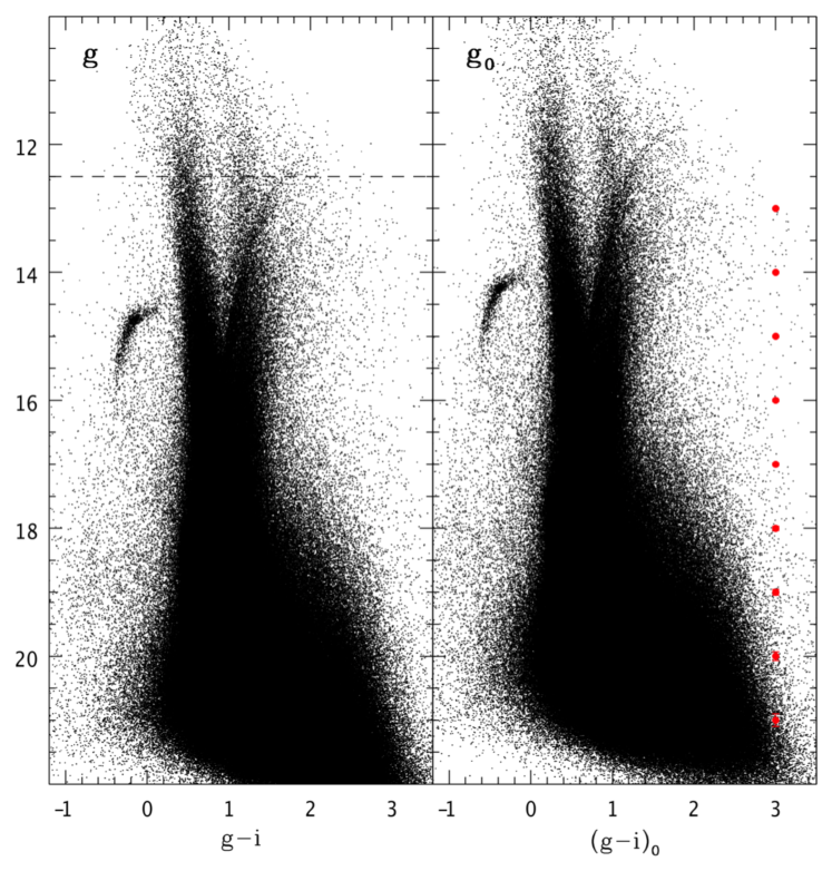
Figure 9: Cumulative CMD for $\omega$ Cen before (left panel) and after (right panel) reddening correction. The red symbols represent the errors at the various luminosity levels. The dashed line represents the CCD nonlinearity limit (see Fig. 4 and text for details)

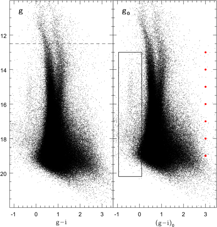
Figure 10: As in Fig. 9 but for NGC6752. The box encloses the vertical structure discussed in the text.

We have used the Schlegel’s maps to obtain a merged total CMD for the surroundings of each cluster with de-reddened magnitude and colors. In Figs. 9 and 10 we report the cumulative CMDs before (left) and after (right) reddening correction. The dashed line indicates the limit of the CCD nonlinearity quoted above.

In the case of Pal 12 (see the bottom panel of Fig. 8) the reddening differences are expected to be very small and we can assume $\Delta$E(B-V) $\sim$ 0 over the entire field. In any case, in the right panel of Fig. 7 we report the de-reddened CMD (black dots) compared with the independent photometry by Stetson (red dots; for details see above). The cluster MSTO is clearly observed from this plot, but a detailed analysis is required in order to disentangle the claimed contribution of the Sagittarius galaxy CMD. For this reason, the investigation of the stellar populations within the observed two tidal radii for this cluster is presented in a separate paper (Di Criscienzo et al. in prep).

For $\omega$ Cen and NGC6752, we checked the internal photometric alignment by using the overlap region of adjacent frames and through over-imposition of the Galactic component features (e.g. the Galactic halo MSTO) in the CMDs within about $\pm$ 0.05 mag.

6.2 Galactic and synthetic cluster model predictions

The observed fields in the direction of $\omega$ Cen and NGC 6752 have low galactic latitude, so that the lines of sight are mainly contaminated by Galactic thin and thick disk stars, with only a minor contribution of halo stars. Although a quantitative interpretation of these populations is beyond the goal of this paper, the simple comparison of the data with the predictions of a Galactic model can be illuminating in the interpretation of the observed CMDs. To this aim we have used an updated version of the code described in Castellani et al. (2002), which assumes three galactic components, namely a thin disk, a thick disk and a stellar halo, with specific spatial structures and star formation laws. The code relies on the latest stellar tracks by Bressan et al. (2012) for normal stars and the theoretical cooling tracks by Salaris et al. (2000) for the white dwarf phase. In this model the Galaxy is described by the following ingredients:

Spatial structure: the thin and thick disk are both described as double exponentials: in Galactocentric distance in the Galactic plane and in height over the plane. The respective scale heights are 250 pc and 750 pc, while the scale lengths are 3 kpc and 3.5 kpc. The halo follows a power-law decay with exponent 3.5 (Cabrera-Lavers et al., 2005; Chen et al., 2001). Thick disk and halo normalizations relative to the thin disk component are 12% (Jurić et al., 2008) and 1/500 (see e.g. Bahcall & Soneira, 1984; Tyson, 1988), respectively;

Star formation laws: for each component the star-formation rate is assumed constant. Stellar ages vary between 0 and 9 Gyr in the thin disk, between 9 and 11 Gyr in the thick disk, and between 11 and 13 Gyr in the halo. The corresponding average metallicities are $Z=0.02$, $Z=0.006$ and $Z=0.0002$, respectively;

Initial Mass Function: all the galactic components assume a Kroupa 2001 Initial Mass Function (IMF, Kroupa, 2001);

We note that some Galactic parameters are still very uncertain, in particular many important details remain to be settled in the thick disk (scale height, normalization and metallicity) and in the halo (normalization) (see e.g. Jurić et al., 2008, and references therein). Hence, the comparison plots we are presenting in the following are not meant to provide a best fit to the data, but only a guide to understand the contribution of the various Galactic populations expected in each field.

6.3 $\omega$ Cen

In the left panel of Fig. 11, we present the de-reddened CMD $g_{0},(g-i)_{0}$ for stars (black dots) in Field #1 (see Fig 2) around $\omega$ Cen compared with the independent photometry for the central region by Castellani et al. (2007, red dots). In the right panel of the figure, we show the results of a Galactic model simulation over 1 deg² centered on the same field (blue, magenta and dark grey symbols represent thin disk, thick disk and halo stars, respectively) compared with the synthetic cluster CMD (red symbols) computed for $\omega$ Cen (see below for details).

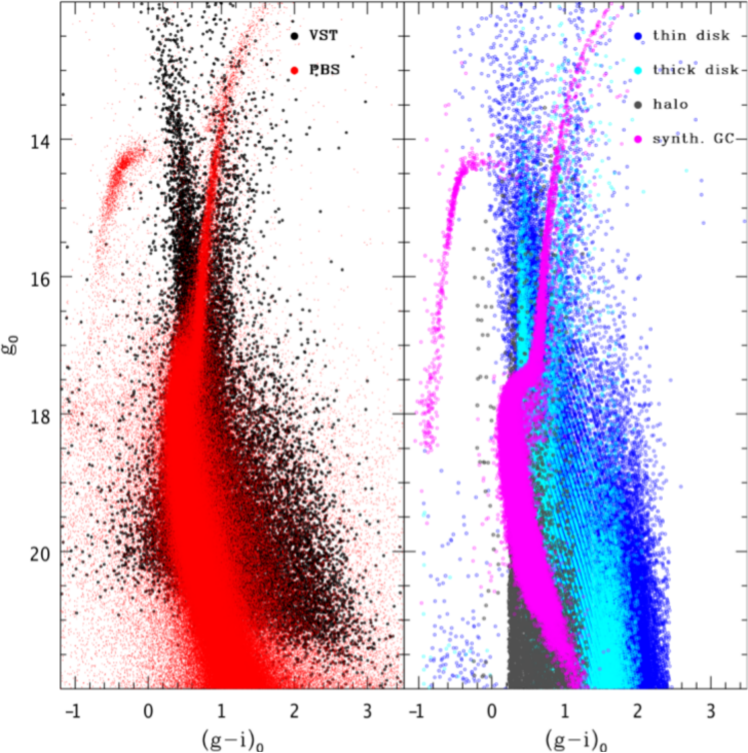
Figure 11: Left panel: CMD of stars observed in Field #1 around $\omega$ Cen (black dots) compared with the transformed central field photometry by Castellani et al. (2007) (red symbols, see text for details). Right panel: the Galactic simulation of the same sky area (blue, cyan and grey symbols represent thin disk, thick disk and halo stars, respectively) discussed in the text compared with the synthetic CMD of $\omega$ Cen (magenta symbols). See text for details.

In the Galactic simulation, the photometric errors are not accounted for. At each given $g$ magnitude, the “blue edge” (the bulk of the bluest stars) can be interpreted as the envelope of the halo MSTO shifted towards fainter magnitudes and redder colors by the increasing distance and corresponding extinction. At the bright end ($g_{0}<16$ mag), the CMD is dominated by thin and thick disk stars. In particular, in this magnitude range, the blue plume (BP; $0<(g-i)_{0}<0.75$ mag) is mainly composed of thin (and a few thick) disk MS stars, whereas the red plume (RP; $1.2<(g-i)_{0}<2.0$ mag) is composed of red giant branch stars of both disks. At fainter magnitudes, the number of thick disk and halo stars increases considerably, until it dominates the star counts for magnitudes fainter than $g_{0}\approx 18$ mag.

To assist in the interpretation of the observations, we also computed the synthetic CMD of $\omega$ Cen from the main-sequence phase up to the asymptotic giant branch phase using the stellar population synthesis code SPoT (Stellar Population Tools, see for details and ingredients Brocato et al., 2000; Raimondo et al., 2005; Raimondo, 2009, and references therein). The synthetic CMDs were randomly populated using Monte Carlo methods with the IMF of Kroupa (2001) in the mass interval 0.1–10 $M_{\sun}$. For each star the luminosity and effective temperature were derived according to evolutionary tracks taken from the BaSTI database, then magnitudes in the ACS/HST (the Advanced Camera for Surveys aboard the Hubble Space Telescope) and Sloan photometric systems were computed, using color-temperature relations derived from the stellar model atmospheres by Castelli & Kurucz (2003, and references therein). In order to reproduce the multipopulations in $\omega$ Cen, we used the subpopulation parameters and ratios suggested by Joo & Lee (2013) as a first guess. Then, we considered the ACS/HST photometry by Sarajedini et al. 2007, and tested on the HST-CMD the bf Horizontal Branch (HB) star distribution as derived from the adopted population ratios. We also explored different assumptions on the parameterizations of the HB star distribution (the Reimers’ mass-loss parameter $\eta_{\rm R}$, its dispersion $\sigma_{\rm R}$, etc; Reimers, 1977). From this procedure we derived our best-fit synthetic CMD for the HST data, which is constructed by assuming the metallicities and ages for six subpopulations, namely: [Z=0.0003, Y=0.245, t=13 Gyr], [Z=0.0006, Y=0.245, t=13 Gyr], [Z=0.0008, Y=0.400, t=12 Gyr], [Z=0.0032 Y=0.400, t=12 Gyr], [Z=0.0065, Y=0.400, t=11.5 Gyr], [Z=0.0165, Y=0.400, t=11 Gyr] (e.g. Joo & Lee, 2013, and references therein). The population ratios are 40%, 27%, 15%, 10%, 7% and 2%, respectively. Note that the adopted metallicity values and abundance ratios agree with the most recent spectroscopic observations of RGB stars in the cluster (e.g. Johnson & Pilachowski, 2010; Marino et al., 2011; Calamida et al., 2009). Each simulation also took into account the photometric error of the adopted HST ACS photometry. We used the same set of parameters to compute the GC CMD in the Sloan filters, also shown in the right panel of Fig. 11. It is worth noting that, according to these simulations, the bluest MSTO might be distinguished from the Galactic disk population (see also discussion in Sect. 7).

6.4 NGC6752

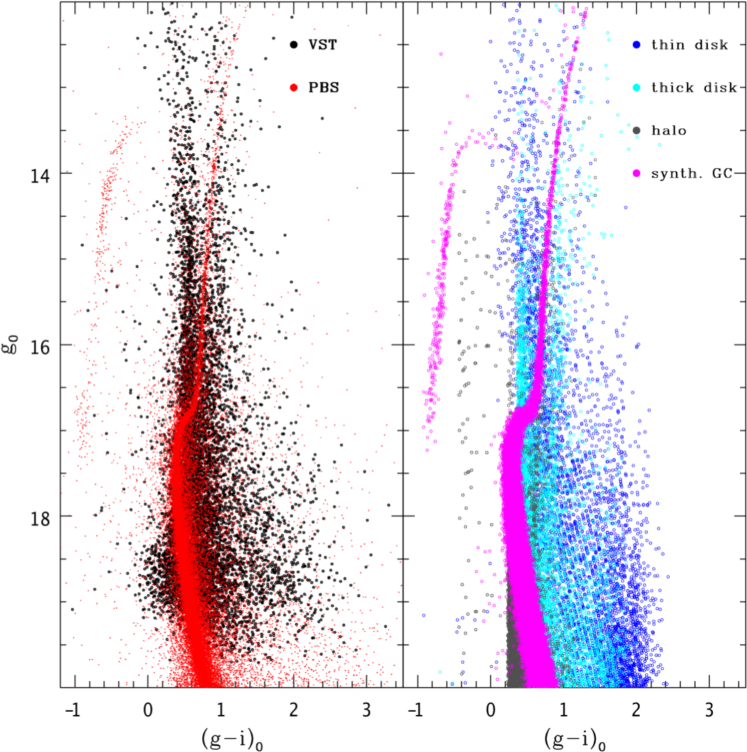
Figure 12: The same of Fig. 11 but for the Field #1 around NGC6752. The photometry of the central area of the cluster is based on PBS unpublished data.

In the left panel of Fig. 12, we present the de-reddened CMD $g_{0},(g-i)_{0}$ for stars (black dots) in Field #1 (see Fig 3) around NGC6752 compared with the independent photometry for the central region by PBS (red dots; for details, see the previous section). In the right panel of the figure, the Galactic simulation for the selected field (same colors as in Fig. 11) is compared with the synthetic CMD, again generated using the SpOT code). This synthetic CMD fits the CMD and the number of HB stars from ACS/HST observations by Sarajedini et al. (2007), considering a single-burst stellar population with $Z=0.0006$, including the $\alpha$ element enhancement (in agreement with the spectroscopic metallicity determination by Gratton et al. (2005) , namely $[Fe/H]=-1.48$ dex and $[\alpha/Fe]=$0.27 dex). We used the same set of parameters to predict the CMD in the Sloan filters, shown in the right panel of Fig. 12. We note that in order to fit the very blue HB of NGC6752 (Buonanno et al., 1986) we fixed the chemical composition and adopted a high value of the Reimers’ parameter $\eta_{R}=0.68$, increasing the mean mass loss along the RGB to $\sim 0.28M_{\odot}$. Alternatively, in the emerging multipopulation scenario for GCs, these stars could be explained assuming they belong to a second generation of stars, with different chemistry (see Milone et al., 2013, and references therein).

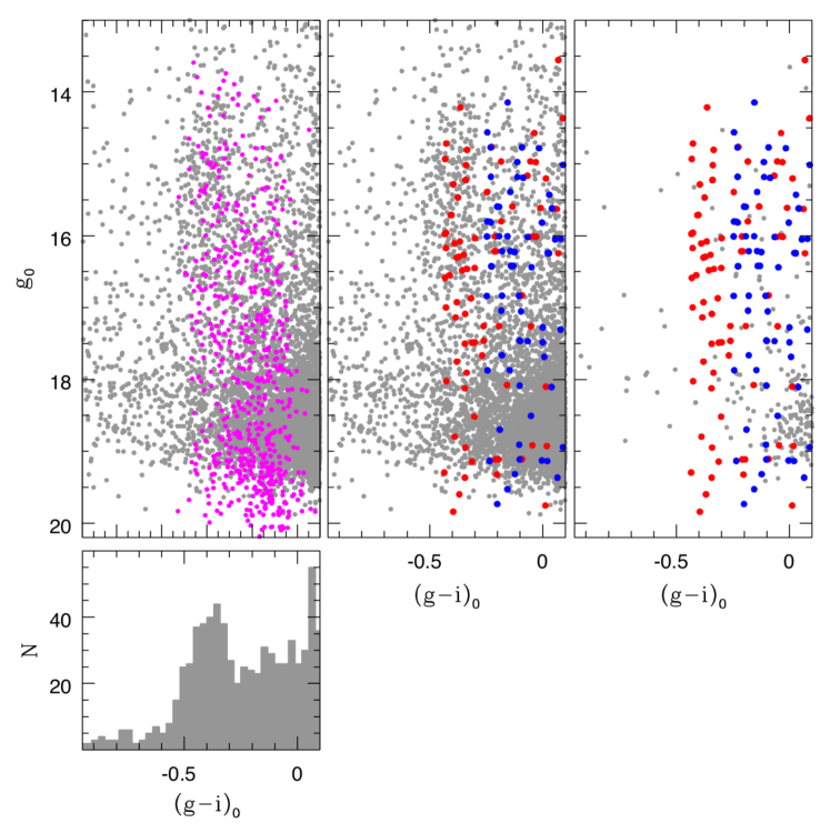
Figure 13: A zoom of the cumulative (left and middle upper panels) and single field (right-upper panel) CMD around NGC6752. The lower panel shows the corresponding $g-i$ color histogram for the cumulative CMD. The magenta dots, in the left panel, represent the SDSS Halo HB stars (see text for details). Red and blue dots, in the middle and right panels, are simulated Halo HB stars adopting different assumptions on the mass loss (see text).

In the CMD of Fig. 10 we can also identify a vertical structure corresponding to $-0.5<(g-i)_{0}<-0.2$ mag and $g_{0}>14$ mag (see box). The stellar nature of all the objects within this structure has been visually verified. Their position in the CMD suggests that they belong to the HB phase associated either with NGC6752 or with the Galactic halo. The comparisons in Fig. 12 show that the observed and predicted colors of the cluster HB stars are much bluer than the average color of the observed vertical structure that is instead reproduced by the Galactic halo simulation. A zoom of this portion of the CMD (box in Fig. 10) is shown in the upper panels of Fig. 13 for the cumulative case (left and middle panels) and Field #1 (right panel), compared with the predicted halo HB stars in this single field. In the lower panel of Fig. 13, we plot the $(g-i)_{0}$ color histogram of this region for the cumulative CMD, showing a clear peak in the color range of the identified structure. In the left upper panel, as an observational check, we compare this feature with the location of the halo HB stars identified by the SDSS (magenta dots; Smith et al., 2010). The good agreement, despite the different areas covered by the two surveys, confirms our hypothesis that these stars belong to the Galactic halo. As a theoretical check, in the middle and right upper panels, we overlaid two halo simulations obtained adopting an RGB mass loss with $\eta_{R}=$ 0.2 (blue dots) and 0.3 (red dots). As expected, the former value produces redder HB stars, as a consequence of the higher average stellar mass populating the synthetic HB. We note that the simulation with $\eta_{R}=0.3$ is more in agreement with the observed vertical structure than the one with $\eta_{R}=0.2$. This discrepancy could be reduced adopting a metallicity value lower than $Z=0.0002$. Concerning the predicted number of HB stars, our models outnumber the observed star counts by roughly a factor two (see Fig. 13). We tentatively ascribe this difference to the assumed halo/thin disk normalization (1/500; e.g. Bahcall & Soneira, 1984; Tyson, 1988), which is probably too high. Indeed, this number is strongly debated and different values have been proposed, i.e., 1/1250 (see e.g. Cohen, 1995), 1/850 (see e.g., Minezaki et al., 1998; Morrison, 1993) or 1/200 (see e.g., Jurić et al., 2008). As a bottom line, we stress how the location and the number of these observed halo HB stars can help to constrain the physical and numerical assumptions adopted in Galactic simulations. In particular, the observed number in our sample seems to suggest a significantly smaller halo/thin disk normalization, close to the lowest values in the literature (Cohen, 1995; Minezaki et al., 1998; Morrison, 1993).

7 Star counts around $\omega$-cen

In this section, we present our analysis of the star counts in the 37 fields covering $\omega$ Cen from the cluster center to about three tidal radii.

The first step to obtain reliable star counts is an evaluation of the photometry completeness in the adopted bands. To this purpose, we adopt the same method used by Coleman et al. (2004, 2005). A luminosity function was generated for each field in both the $g$ and $i$ bands adopting a magnitude bin of 0.2 mag. We then assumed the completeness limit of each field to be 0.2 mag brighter than the turnover in the luminosity function. The overall magnitude limit of the survey, for each group of fields, is then defined by the field with the shallowest depth. For $\omega$ Cen we obtain the limit magnitudes of $g_{0}=19.4$ mag and $i_{0}=18.4$ mag from the luminosity function of the shallowest field (shown in the left panel of Fig. 14). In the right panel of the figure, we plot the luminosity functions obtained from one of the many fields observed in good seeing conditions (as an example field #32), to conclude that these fields observed in good weather conditions can be considered complete down to $g_{0}=20.8$ mag and $i_{0}=19.4$ mag.

Figure 14: Luminosity function of stars in Field #33 (left panel) and #32 (right panel) around $\omega$ Cen with a magnitude bin of 0.2 mag.

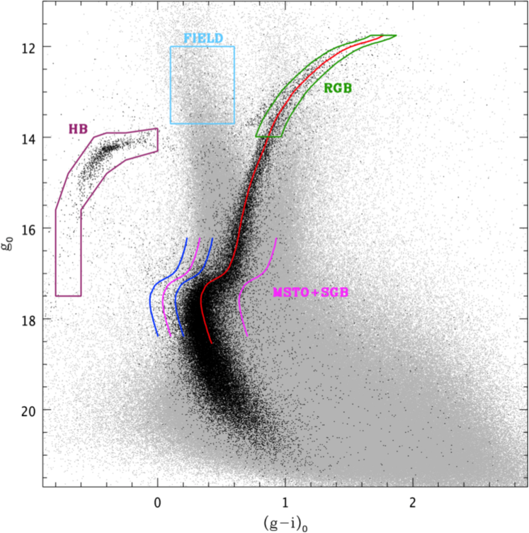
Figure 15: Central CMD (black dots) for $\omega$ Cen compared with the cumulative one (grey dots). The over-imposed red line is the empirical ridgeline. Stellar evolutionary phases and a FIELD region are labelled (see text for details).

A method to search for stellar over-densities is deriving star counts in specific CMD regions. The availability of the central fields, allowed us to use the 1 square degree CMD centered on $\omega$ Cen (hereinafter “central CMD”) to define the expected location of the HB, MSTO and RGB phases. In Fig. 15, we show the central CMD (black dots) compared with the total CMD of Fig. 9 (grey dots). The red line represents the empirical ridge-line obtained from the observed central CMD. After this procedure, we conservatively selected as possible members of the cluster the sources lying within a defined color range around the ridge line, that is:

• $\pm 0.1$ mag, with $g_{0}<14$ mag and $(g-i)_{0}>0.7$ mag, for the RGB (region inside the green contour line),

• $\pm 0.3$ mag (between the blue lines, to account for the dispersion of the MSTO region and for possible photometric misalignment due to residual differential reddening and/or photometric errors), with $16.2<g_{0}<18.5$ mag, for the MSTO and the Sub Giant Branch (labelled in the following as MSTO+SGB).

For the HB phase, due to its specific morphology, different ranges in magnitude and color were considered in order to properly cover the whole extent (region inside the purple contour line). In this CMD, we also identified a region without cluster contamination (region inside light blue contour line labelled as FIELD), corresponding to $12.0<g_{0}<13.7$ mag and $0.1<(g-i)_{0}<0.6$ mag, to quantify the contribution due to the Galactic thin and thick disk (see right panel of Fig. 11).

Figure 16: Radial profiles of the normalized (see text for details) star densities, in logarithmic scale, for $\omega$ Cen (selected from the CMD $g$ vs $g-i$), in the three labelled evolutionary phases (HB, RGB, MSTO+SGB) compared with the results in the FIELD region. The dashed line represents the nominal tidal radius, whereas the solid line, in the upper right panel, represents the King profile based on Harris (1996) values.

Figure 17: A zoom-in of Fig.16 in the region around the nominal tidal radius.

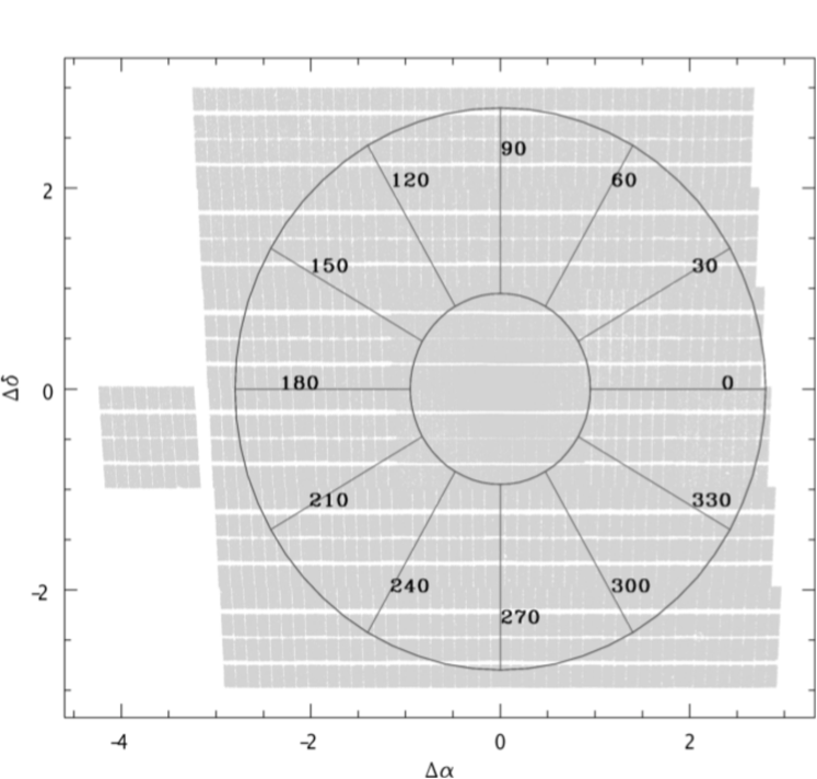
Figure 18: Schematic view of the circular sectors used for angular star counts.

In the panels of Fig. 16 we plot the radial profiles of the normalized star densities in the three evolutionary phases mentioned (HB, RGB, MSTO+SGB) compared to those in the FIELD region where we expect a negligible contribution of cluster stars. We adopted 75 equally spaced annuli, from the center up to 2.8 deg, corresponding to about 3 tidal radii. For each selected evolutionary phase, star density in the $i$-th annulus is normalized to the corresponding total value computed in the circle with the radius of 2.8 deg. The vertical dashed line represents the nominal tidal radius of 0.95 deg (Harris, 1996; Da Costa & Coleman, 2008), that is intermediate between the two values provided by McLaughlin & van der Marel (2005) adopting a King model (0.80 deg; King, 1966) and a Wilson model (1.2 deg; Wilson, 1975). We remind that the measurement of the tidal radius is significantly model-dependent (McLaughlin & van der Marel, 2005) and difficult to obtain on the basis of simple structural models due to the possible presence of tidal tails or other kinds of extra-tidal stellar population (see e.g. Di Cecco et al., 2013, and references therein). In Fig. 16, the error bars result from the propagation of the Poisson errors on the individual counts. A zoom of these plots to emphasize the behavior around the tidal radius is shown in Fig. 17. As expected, the FIELD stars do not show any specific trend, whereas in the other three cases, we obtain the typical expected profile for a globular cluster (e.g. King, 1966; Wilson, 1975, see discussion below). This is shown in the right upper panel of Fig.  16 where the King profile based on Harris (1996) values (solid line) is overimposed on the MSTO+SGB star counts. However, an inspection of Fig. 17 suggests that, apart from the poorly populated HB phase, the nominal tidal radius seems to be slightly underestimated with an excess of stars at this distance from the center, suggesting a better agreement with the value based on the Wilson model (1.2 deg McLaughlin & van der Marel, 2005). Moreover, we notice a non-negligible increase of the density around and beyond 2 tidal radii, both for RGB and MSTO+SGB stars, thus not excluding the presence of extra-tidal cluster stars. However, the RGB counts are affected by large errors due to the smaller statistics, and for this reason, in the following, we concentrate on the much more numerous MSTO+SGB stars. To further investigate the possible presence of tidal tails, we also considered the MSTO+SGB star counts as a function of the direction. To this purpose, we divided the total explored area into twelve 30 deg circular sectors (see Fig. 18) and counted the MSTO+SGB stars within each sector with a radial distance ranging from 1 to 3 tidal radii. The results are shown in the lower panel of Fig. 19, where star counts are normalized to the total number of stars in the same area. This normalization allows us to reduce spurious effects related to the differential contribution of the disk population that is expected to be more important at lower galactic latitudes (see discussion in section 6). In Fig. 20, we present the same plot, but considering a different selection of the MSTO+SGB stars, labelled as asymmetric, that includes stars bluer than the ridgeline by 0.2 to 0.4 mag (region between the blue lines in Fig. 15) with magnitude fainter than 17 mag. This selection has the drawback of containing a lower number of stars, but the advantage of reducing the disk contamination, instead including the cluster MSTO stars emerging from the disk population as shown in Fig. 15. In the upper panel of Figs. 19 and 20, we show for comparison the behavior of the same normalized counts for the FIELD stars defined above, adopting the same vertical scale used for the lower panel. We emphasize that in both figures, the MSTO+SGB star counts show a clear peak around 300 deg (the south-east direction), corresponding to the predicted ellipticity orientation of the cluster (see e.g. Table 5 in Anderson & van der Marel, 2010). Even if the asymmetric selection is less statistically significant, it is interesting to note that the trend is the same and that this effect cannot be related to a larger disk contribution in this direction because FIELD stars show an opposite behavior.

Figure 19: Normalized (see text for detail) star counts for $\omega$ Cen (selected from the CMD $g$ vs $g-i$) in circular sectors for stars in the MSTO+SGB phase within $\pm 0.3$ mag from the ridgeline (lower panel) and in the FIELD region (upper panel).

Figure 20: Normalized (see text for detail) star counts for $\omega$ Cen (selected from the CMD $g$ vs $g-i$) in circular sectors for stars in the MSTO+SGB phase, bluer than the ridgeline by 0.3 to 0.4 mag and fainter than 17 mag (lower panel, labelled as “asymmetric”) and in the FIELD region (upper panel).

The contribution of this direction to the detected extra-tidal overdensity is also evident from Fig. 21 where we compare the obtained radial profile for MSTO+SGB stars (black filled circles) with the ones obtained considering the overdensity direction (blue open circles) and its complement to $2\pi$ (red open circles), respectively. We note that: i) the radial profile varies with the selected angle with the overdensity detected beyond the tidal radius mainly due to stars concentrated in the south-east direction; ii) even excluding the over-density direction, the radial profile (red open circles) indicates a tidal radius of about 1.2 deg, with an excess of stars at about 1 deg from the center.

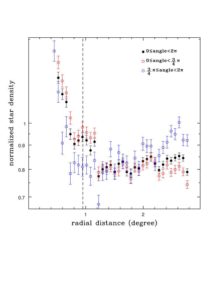
Figure 21: Radial profiles of the normalized star densities, in logarithmic scale, for the $\omega$ Cen MSTO+SGB stars in the labelled angular regions.

To further constrain the nature of the candidate cluster stars located beyond the truncation radius we decided to adopt the contour levels. Fig. 22 shows the count levels for the MSTO+SGB ($\pm 0.3$ mag) candidate cluster stars (red dots). In order to overcome the steady increase in the counts of field stars when moving from the northern to the southern direction we performed a simultaneous fit of a surface and a plane. We divided the sky area covered by the data into a grid (800$\times$800) and subtracted point-by-point the plane from the surface. The contour levels plotted in the above figure display several interesting features.

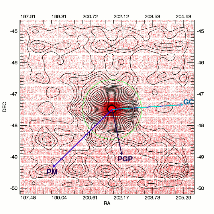
Figure 22: Contour levels of candidate $\omega$ Cen stars projected onto the sky. The coordinates and the orientation are the same as in Fig.2. The red dots display the radial distribution of the entire photometric catalog. The black contours show different density level after the subtraction of a plane. The green circle shows the truncation radius ($r_{t}$=0.95 deg). The light blue arrow points to the Galactic Center (GC), the purple arrow points to the direction of the proper motion of the cluster (PM), while the blue arrow the direction perpendicular to the Galactic Plane (PGP). Note the clear excess of star across and beyond the truncation radius and the over-densities located in the fourth and in the second quadrants. See text for more details.

i) – The countour levels display a well defined excess of star counts beyond the truncation radius (green circle, $r_{t}$=0.95 deg). This evidence is clearer in the II, III and IV quadrants where the excess extends up to two truncation radii. This finding soundly confirms the evidence of extra-tidal stars based on the radial density profile.

ii) – The contour levels become less and less symmetric when moving from the innermost to the outermost cluster regions, in good agreement with the eccentricity of $\omega$ Cen provided by Bianchini et al. (2013).

iii) – The countour levels display a clear over-density when moving from the bottom right to the top left, even if the over-density is less clear in the II than in the IV quadrant. It is worth mentioning that these overdensities appear to be orthogonal to the direction of the proper motion of the cluster (PM, purple arrow; van Leeuwen et al., 2000; van de Ven et al., 2006) and located between the direction of the Galactic Center (GC, light blue arrow) and the projection on the sky of the direction perpendicular to the Galactic Plane (PGP, black arrow).

iv) – The countour levels indicate that the position angle of the major axis measured east from north is $\sim 140$ degrees. The current estimate agrees quite well with the determination based on ACS photometry of the innermost cluster regions provided by Anderson & van der Marel (2010).

The above empirical evidence indicates that candidate cluster stars have a complex distribution at radial distances larger than two tidal radii. Firmer conclusions concerning the nature of the extra-tidal stars are hampered by the lack of information concerning their proper motion and radial velocity.

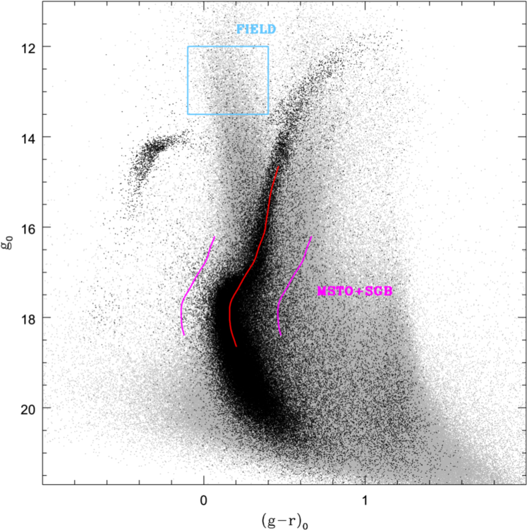
Figure 23: Central CMD in $g$ vs $g-r$ (black dots) for $\omega$ Cen compared with the cumulative one (grey dots). The over-imposed red line is the empirical ridgeline. The MSTO+SGB phase (within the two magenta lines) and a FIELD region (cyan box) are labelled (see text for details).

Figure 24: Left panels: radial profiles of the normalized (see text for details) star densities, in logarithmic scale, for $\omega$ Cen (selected from the CMD $g$ vs $g-r$) in the MSTO+SGB evolutionary phase compared with the results in the FIELD region. Right panels: a zoom-in of the left panels around the nominal tidal radius (dashed line).

As a check of the results obtained in the $g,i$ filters, we perform a star-count analysis also in the $g$ vs $g-r$ CMD, but only in the more populous MSTO+SGB region. Figure 23 shows the CMD obtained in these filters and the selected regions for star counts around the cluster MSTO+SGB ($\pm$ 0.3 mag, magenta lines) and in the FIELD (light blue box). These star counts are used to build the radial profile (see Fig. 24) and the angular distribution (see Fig. 25) in analogy with the procedure adopted in the $g$ and $i$ filters. The left panels of Fig. 24 show the normalized star density as a function of the radial distance from the cluster center in the MSTO+SGB region (upper panel) and in the FIELD zone (lower panel). The right panels show the corresponding zoom plots. These results confirm the evidence, discussed above, that the cluster tidal radius is closer to the estimate based on the Wilson model than to the nominal value (dashed line). The angular distribution shown in Fig. 25 supports the evidence of an overdensity in the same directions identified in Fig. 19.

Figure 25: Normalized star counts for $\omega$ Cen (selected from the CMD in $g$ vs $g-r$), in circular sectors for stars in the MSTO+SGB phase within $\pm 0.3$ mag from the ridgeline (lower panel) and in the FIELD region (upper panel).

These results seem to suggest the presence of a tidal tail in addition to a general extension of the cluster beyond the traditionally assumed tidal radius. We notice that the presence of extra tidal stars support previous evidence by Meza et al. (2005) concerning a peak of angular momentum, consistent with that of $\omega$ Cen, identified in the stellar samples by Beers et al. (2000) and Gratton et al. (2003).

A similar behavior was also claimed by Majewski et al. (2012) with the direction of the $\omega$ Cen debris mentioned in their paper consistent with the one identified in this paper (see Fig. 1a in Majewski et al., 2012). Obviously, these preliminary results need additional investigation and spectroscopic confirmation.

8 Summary and Future Perspectives

We have presented an overview of the STREGA survey on the VST Guaranteed Time, focused on a multifilter photometric investigation of selected regions of the Galactic halo. The core program of the survey is focused on the investigation of neighboring areas of a number of GGCs and dSphs reaching at least 2 tidal radii in different directions with the final aim of detecting extratidal stellar populations either in tails or in extended haloes. The adopted stellar tracers of streams and haloes are both MSTO and variable stars but so far only runs involving the former have been completed, and data reduction and analysis performed, for three GGCs, namely $\omega$ Cen, NGC6752 and Pal 12. For the first two systems we have also performed a comparison with model predictions and discussed some preliminary results. The most relevant ones are:

• A possible structure of Galactic halo HB stars is present in the CMD around NGC6752, barely consistent with the presence of cluster HB stars, and their number and location can be used to constrain the assumptions of Galactic models. The observation of the four central square degrees of NGC6752 in the next ESO Period of observation will allow us to produce the radial profile of star counts in the CMD and to investigate in detail the possible presence of tidal tails and/or of an extended halo around this system;

• We confirm that the nominal tidal radius for $\omega$ Cen seems to be underestimated, suggesting a value more in agreement with 1.2 deg as based on the Wilson model.

• We find evidence of stellar over-density around $\omega$ Cen at about 1 deg from the center in the North-West direction and at about 2 deg in the opposite direction. The resulting asymmetric, elongated extra-tidal structure seems to be consistent with the extension to longer radial distances of current measurements and predictions for the cluster ellipticity profile and orientation.

In the case of Pal 12 the interpretation of the CMD and the star count investigation is in progress (Di Criscienzo et al. in prep). In the next two periods of observations (ESO P93 and P94) the time-series data of the selected fields for Pal 3, Fornax, and Sculptor should be completed and we will be able to use RR Lyrae stars in combination with MSTO stars to identify extratidal stellar populations around these systems, up to at least three tidal radii. The narrow band observations for the WDs and IBs in the Pal 3 fields will also be performed. In the subsequent two semesters we plan to extend the analysis to Phoenix and Sextans, thus completing the core program of the Survey.

9 Acknowledgments

We thank our anonymous referee for her/his valuable comments and suggestions. This work was supported by PRIN–INAF 2011 “Tracing the formation and evolution of the Galactic halo with VST” (PI: M. Marconi), PRIN-INAF 2011 “Galaxy Evolution with the VLT Surveys Telescope (VST)” (PI: A. Grado) and PRIN–MIUR (2010LY5N2T) “Chemical and dynamical evolution of the Milky Way and Local Group galaxies” (PI: F. Matteucci). MDC acknowledges the support of INAF through the 2011 postdoctoral fellowship grant on the STREGA survey.

References

- Andersen et al. (1995) Andersen, M. I.; Freyhammer, L.; Storm, J. 1995, ESO Conference, 53, 87
- Anderson & van der Marel (2010) Anderson, J., & van der Marel, R. P. 2010, ApJ, 710, 1032
- Arnaboldi et al (2008) Arnaboldi, M., Dietrich, J., Hatziminaoglou, E., et al., 2008, The Messenger, 134, 42
- Bahcall & Soneira (1984) Bahcall, J. N.; Soneira, R. M., 1984, ApJS, 55, 67B
- Beers et al. (2000) Beers, T. C., Chiba, M., Yoshii, Y., et al. 2000, AJ, 119, 2866
- Bell et al. (2010) Bell, E. F., Xue, X. X., Rix, H.-W., Ruhland, C., & Hogg, D. W. 2010, AJ, 140, 1850
- Bellazzini et al. (2006) Bellazzini, M., Newberg, H. J., Correnti, M., Ferraro, F. R., & Monaco, L. 2006, A&A, 457, L21
- Bellazzini et al. (2003) Bellazzini, M., Ibata, R., Ferraro, F. R., & Testa, V. 2003, Astronomy & Astrophysics, 405, 577
- Belokurov et al. (2006) Belokurov, V., Zucker, D. B., Evans, N. W., et al. 2006, ApJL, 647, L111
- Belokurov et al. (2007) Belokurov, V., Zucker, D. B., Evans, N. W., et al. 2007, ApJ, 654, 897
- Benson et al. (2002) Benson, A. J., Ellis, R. S., & Menanteau, F. 2002, MNRAS, 336, 564
- Bertin & Arnouts (1996) Bertin, E. & Arnouts, S., 1996, A&AS, 117,393B
- Bertin (2006) Bertin, E., 2006, ASP Conference Series, 351, 112
- Bertin (2002) Bertin et al. 2002, ASP Conference Series, Vol. 281, 2002 D.A. Bohlender, D. Durand, and T.H. Handley, eds., p. 228
- Bianchini et al. (2013) Bianchini, P., Varri, A. L., Bertin, G., & Zocchi, A. 2013, ApJ, 772, 67
- Bressan et al. (2012) Bressan, Alessandro; Marigo, Paola; Girardi, Léo.; Salasnich, Bernardo; Dal Cero, Claudia; Rubele, Stefano; Nanni, Ambra, 2012, MNRAS, 427, 127B
- Brocato et al. (2000) Brocato, E.; Castellani, V.; Poli, F. M.; Raimondo, G., 2000, A&AS, 146, 91B
- Buonanno et al. (1986) Buonanno, R.; Caloi, V.; Castellani, V.; Corsi, C.; Fusi Pecci, F.; Gratton, R., 1986, A&AS, 66, 79B
- Cabrera-Lavers et al. (2005) Cabrera-Lavers, A., Garzón, F., & Hammersley, P. L. 2005, A&A, 433, 173
- Calamida et al. (2009) Calamida, A., Bono, G., Stetson, P. B., et al. 2009, ApJ, 706, 1277
- Capaccioli & Schipani (2011) Capaccioli, M. & Schipani, P. 2011, The Messenger, 146, 2
- Carollo et al. (2007) Carollo, D., Beers, T. C., Lee, Y. S., et al. 2007, Nature, 450, 1020
- Carretta (2013) Carretta, E. 2013, Astronomy & Astrophysics, 557, A128
- Castelli & Kurucz (2003) Castelli, F., & Kurucz, R. L. 2003, Modelling of Stellar Atmospheres, 210, 20P
- Castellani et al. (2002) Castellani, V.; Cignoni, M.; Degl’Innocenti, S.; Petroni, S.; Prada Moroni, P. G., 2002, MNRAS, 334, 69C
- Castellani et al. (2007) Castellani, V., Calamida, A., Bono, G., et al. 2007, ApJ, 663, 1021
- Chen et al. (2001) Chen, B., Stoughton, C., Smith, J. A., et al. 2001, ApJ, 553, 184
- Chun et al. (2010) Chun, S.-H., Kim, J.-W., Sohn, S. T., et al. 2010, AJ, 139, 606
- Cignoni et al. (2007) Cignoni, M., Ripepi, V., Marconi, M., et al. 2007, A&A, 463, 975
- Clementini et al. (2011) Clementini, G., Contreras Ramos, R., Federici, L., et al. 2011, ApJ, 743, 19
- Clementini et al. (2012) Clementini, G., Cignoni, M., Contreras Ramos, R., et al. 2012, ApJ, 756, 108
- Cohen (1995) Cohen, M. 1995, ApJ, 444, 874
- Cohen (2004) Cohen, J. G. 2004, AJ, 127, 1545
- Coleman et al. (2004) Coleman, M., Da Costa, G. S., Bland-Hawthorn, J., et al. 2004, AJ, 127, 832
- Coleman et al. (2005) Coleman, M. G., Da Costa, G. S., Bland-Hawthorn, J., & Freeman, K. C. 2005, AJ, 129, 1443
- Conn et al. (2013) Conn, A. R., Lewis, G. F., Ibata, R. A., et al. 2013, ApJ, 766, 120
- Da Costa & Coleman (2008) Da Costa, G. S., & Coleman, M. G. 2008, AJ, 136, 506
- Dall’Ora et al. (2006) Dall’Ora, M., Clementini, G., Kinemuchi, K., et al. 2006, ApJL, 653, L109
- Dall’Ora et al. (2012) Dall’Ora, M., Kinemuchi, K., Ripepi, V., et al. 2012, ApJ, 752, 42
- Da Costa (1999) Da Costa, G. S. 1999, The Third Stromlo Symposium: The Galactic Halo, 165, 153
- Deg & Widrow (2013) Deg, N., & Widrow, L. 2013, MNRAS, 428, 912
- De Gennaro et al. (2008) De Gennaro, S., von Hippel, T., Winget, D. E., et al. 2008, AJ, 135, 1
- Del Principe et al. (2006) Del Principe, M., Piersimoni, A. M., Storm, J., et al. 2006, ApJ, 652, 362
- Demers & Kunkel (1979) Demers, S., & Kunkel, W. E. 1979, PASP, 91, 761
- Di Cecco et al. (2013) Di Cecco, A., Zocchi, A., Varri, A. L., et al. 2013, AJ, 145, 103
- Dinescu et al. (1999) Dinescu, D. I., Girard, T. M., & van Altena, W. F. 1999, AJ, 117, 1792
- Dinescu et al. (2004) Dinescu, D. I., Keeney, B. A., Majewski, S. R., & Girard, T. M. 2004, AJ, 128, 687
- Drake et al. (2013) Drake, A. J., Catelan, M., Djorgovski, S. G., et al. 2013, ApJ, 765, 154
- Drew et al. (2014) Drew, J. E., Gonzalez-Solares, E., Greimel, R., et al. 2014, arXiv:1402.7024
- Drukier et al. (2003) Drukier, G. A., Bailyn, C. D., Van Altena, W. F., & Girard, T. M. 2003, AJ, 125, 2559
- Fellhauer et al. (2007) Fellhauer, M., Evans, N. W., Belokurov, V., Wilkinson, M. I., & Gilmore, G. 2007, MNRAS, 380, 749
- Gänsicke et al. (2009) Gänsicke, B. T., Dillon, M., Southworth, J., et al. 2009, MNRAS, 397, 2170
- Garofalo et al. (2013) Garofalo, A., Cusano, F., Clementini, G., et al. 2013, ApJ, 767, 62
- Gilbert et al. (2009) Gilbert, K. M., Font, A. S., Johnston, K. V., & Guhathakurta, P. 2009, ApJ, 701, 776
- Grado et al. (2012) Grado, A., Capaccioli, M., Limatola, L., & Getman, F. 2012, Memorie della Societa Astronomica Italiana Supplementi, 19, 362
- Gratton et al. (2003) Gratton, R. G., Carretta, E., Claudi, R., Lucatello, S., & Barbieri, M. 2003, A&A, 404, 187
- Gratton et al. (2005) Gratton, R. G., Bragaglia, A., Carretta, E., et al. 2005, A&A, 440, 901
- Harris (1996) Harris, W.E. 1996, AJ, 112, 1487
- Hayashi et al. (2003) Hayashi, E., Navarro, J. F., Taylor, J. E., Stadel, J., & Quinn, T. 2003, ApJ, 584, 541
- Ibata et al. (1994) Ibata, R. A., Gilmore, G., & Irwin, M. J. 1994, Nature, 370, 194
- Ibata et al. (2013) Ibata, R. A., Lewis, G. F., Conn, A. R., et al. 2013, Nature, 493, 62
- Irwin & Hatzidimitriou (1995) Irwin, M., & Hatzidimitriou, D. 1995, MNRAS, 277, 1354
- Irwin (1999) Irwin, M. 1999, The Stellar Content of Local Group Galaxies, 192, 409
- Ivezic et al. (2004) Ivezic, Z., Lupton, R., Schlegel, D., et al. 2004, Milky Way Surveys: The Structure and Evolution of our Galaxy, 317, 179
- Johnson & Pilachowski (2010) Johnson, C. I., & Pilachowski, C. A. 2010, ApJ, 722, 1373
- Joo & Lee (2013) Joo, S.-J., & Lee, Y.-W. 2013, ApJ, 762, 36
- Jordi et al. (2006) Jordi, K., Grebel, E. K., & Ammon, K. 2006, A&A, 460, 339
- Jurić et al. (2008) Jurić, M., Ivezić, Ž., Brooks, A., et al. 2008, ApJ, 673, 864
- King (1966) King, I. R. 1966, AJ, 71, 64
- Kroupa (2001) Kroupa, P. 2001, MNRAS, 322, 231
- Kuijken (2011) Kuijken, K. 2011, The Messenger, 146, 8
- Kuhn et al. (1996) Kuhn, J. R., Smith, H. A., & Hawley, S. L. 1996, ApJL, 469, L93
- Lane et al. (2012a) Lane, R. R., Küpper, A. H. W., & Heggie, D. C. 2012a, MNRAS, 423, 2845
- Lane et al. (2012b) Lane, R. R., Küpper, A. H. W., & Heggie, D. C. 2012b, MNRAS, 426, 797
- Law et al. (2003) Law, D. R., Majewski, S. R., Skrutskie, M. F., Carpenter, J. M., & Ayub, H. F. 2003, AJ, 126, 1871
- Leon et al. (2000) Leon, S., Meylan, G., & Combes, F. 2000, A&A, 359, 907
- López-Corredoira et al. (2007) López-Corredoira, M., Momany, Y., Zaggia, S., & Cabrera-Lavers, A. 2007, A&A, 472, L47
- Lynden-Bell (1976) Lynden-Bell, D. 1976, MNRAS, 174, 695
- Lynden-Bell (1982) Lynden-Bell, D. 1982, The Observatory, 102, 202
- Lynden-Bell & Lynden-Bell (1995) Lynden-Bell, D., & Lynden-Bell, R. M. 1995, MNRAS, 275, 429
- Madau et al. (2008) Madau, P., Diemand, J., & Kuhlen, M. 2008, ApJ, 679, 1260
- Majewski (1994) Majewski, S. R. 1994, ApJL, 431, L17
- Majewski et al. (2000) Majewski, S. R., Ostheimer, J. C., Patterson, R. J., et al. 2000, AJ, 119, 760
- Majewski et al. (2003) Majewski, S. R., Skrutskie, M. F., Weinberg, M. D., & Ostheimer, J. C. 2003, ApJ, 599, 1082
- Majewski et al. (2012) Majewski, S. R., Nidever, D. L., Smith, V. V., et al. 2012, ApJL, 747, L37
- Marconi et al. (2014) Marconi, M., Musella, I., Di Criscienzo, M. et al. 2014 ASP Conf. Series, in press
- Marino et al. (2011) Marino, A. F., Milone, A. P., Piotto, G., et al. 2011, ApJ, 731, 64
- Martin et al. (2004) Martin, N. F., Ibata, R. A., Bellazzini, M., et al. 2004, MNRAS, 348, 12
- Martínez-Delgado et al. (2002) Martínez-Delgado, D., Zinn, R., Carrera, R., & Gallart, C. 2002, ApJL, 573, L19
- Mateo (1998) Mateo, M. L. 1998, ARA&A, 36, 435
- Mateo et al. (2008) Mateo, M., Olszewski, E. W., & Walker, M. G. 2008, ApJ, 675, 201
- Mateu et al. (2009) Mateu, C., Vivas, A. K., Zinn, R., Miller, L. R., & Abad, C. 2009, AJ, 137, 4412
- Mayer et al. (2002) Mayer, L., Moore, B., Quinn, T., Governato, F., & Stadel, J. 2002, MNRAS, 336, 119
- Mayer (2011) Mayer, L. 2011, EAS Publications Series, 48, 369
- McLaughlin & van der Marel (2005) McLaughlin, D. E., & van der Marel, R. P. 2005, ApJS, 161, 304
- Meza et al. (2005) Meza, A., Navarro, J. F., Abadi, M. G., & Steinmetz, M. 2005, MNRAS, 359, 93
- Milone et al. (2013) Milone, A. P., Marino, A. F., Piotto, G., et al. 2013, ApJ, 767, 120
- Minezaki et al. (1998) Minezaki, T., Yoshii, Y., Majewski, S. R., Zaggia, S., et al. 2006, ApJ, 649, 201
- Mirabel et al. (2001) Mirabel, I. F., Dhawan, V., Mignani, R. P., Rodrigues, I., & Guglielmetti, F. 2001, Nature, 413, 139
- Momany et al. (2006) Momany, Y., Zaggia, S., Gilmore, G., et al. 2006, A&A, 451, 515
- Monelli et al. (2004) Monelli, M., Walker, A. R., Bono, G., et al. 2004, Memorie della Societa Astronomica Italiana Supplementi, 5, 65
- Moretti et al. (2009) Moretti, M. I., Dall’Ora, M., Ripepi, V., et al. 2009, ApJ, 699, L125
- Morrison (1993) Morrison, H. L. 1993, AJ, 106, 578
- Muñoz et al. (2006) Muñoz, R. R., Majewski, S. R., Zaggia, S., et al. 2006, ApJ, 649, 201
- Musella et al. (2009) Musella, I., Ripepi, V., Clementini, G., et al. 2009, ApJL, 695, L83
- Musella et al. (2012) Musella, I., Ripepi, V., Marconi, M., et al. 2012, ApJ, 756, 121
- Navarro et al. (1997) Navarro, J. F., Frenk, C. S., & White, S. D. M. 1997, ApJ, 490, 493
- Newberg et al. (2003) Newberg, H. J., Yanny, B., Grebel, E. K., et al. 2003, ApJL, 596, L191
- Odenkirchen et al. (2001) Odenkirchen, M., Grebel, E. K., Rockosi, C. M., et al. 2001, ApJL, 548, L165
- Odenkirchen et al. (2001) Odenkirchen, M., Grebel, E. K., Rockosi, C. M., et al. 2001, ApJL, 548, L165
- Odenkirchen et al. (2009) Odenkirchen, M., Grebel, E. K., Kayser, A., Rix, H.-W., & Dehnen, W. 2009, AJ, 137, 3378
- Olszewski et al. (2009) Olszewski, E. W., Saha, A., Knezek, P., et al. 2009, AJ, 138, 1570
- Patterson et al. (2008) Patterson, J., Thorstensen, J. R., & Knigge, C. 2008, PASP, 120, 510
- Pawlowski et al. (2012) Pawlowski, M. S., Pflamm-Altenburg, J., & Kroupa, P. 2012, MNRAS, 423, 1109
- Pawlowski & Kroupa (2013) Pawlowski, M. S., & Kroupa, P. 2013, MNRAS, 435, 2116
- Prior et al. (2009) Prior, S. L., Da Costa, G. S., & Keller, S. C. 2009, ApJ, 704, 1327
- Radovich et al. (2004) Radovich, M., Arnaboldi, M., Ripepi, V., et al. 2004, A&A, 417, 51
- Raimondo et al. (2005) Raimondo, G., Brocato, E., Cantiello, M., & Capaccioli, M. 2005, AJ, 130, 2625
- Raimondo (2009) Raimondo, G., 2009, ApJ, 700, 1247R
- Read et al. (2006) Read, J. I., Wilkinson, M. I., Evans, N. W., Gilmore, G., & Kleyna, J. T. 2006, MNRAS, 367, 387
- Reimers (1977) Reimers, D. 1977, A&A, 61, 217
- Richardson et al. (2008) Richardson, J. C., Ferguson, A. M. N., Johnson, R. A., et al. 2008, AJ, 135, 1998
- Rosenberg et al. (1998) Rosenberg, A., Saviane, I., Piotto, G., &Held, E. V. 1998, A&A, 339, 61
- Rowell & Hambly (2011) Rowell, N., & Hambly, N. C. 2011, MNRAS, 417, 93
- Saviane et al. (2011) Saviane, I., Monaco, L., Correnti, M., Bonifacio, P., & Geisler, D. 2011, EAS Publications Series, 48, 251
- Salaris et al. (2000) Salaris, M.; García-Berro, E.; Hernanz, M.; Isern, J.; Saumon, D., 2000, ApJ, 544, 1036S
- Sarajedini et al. (2007) Sarajedini, et al. 2007, AJ, 133, 1658
- Schlafly & Finkbeiner (2011) Schlafly, E. F., & Finkbeiner, D. P. 2011, ApJ, 737, 103
- Schlegel et al. (1998) Schlegel, David J.; Finkbeiner, Douglas P.; Davis, Marc, 1998ApJ, 500, 525S
- Smith et al. (2002) Smith J.A., Tucker D.L., Kent S., et al. 2002, AJ, 123, 2121
- Smith et al. (2010) Smith, K. W., Bailer-Jones, C. A. L., Klement, R. J., & Xue, X. X. 2010, VizieR Online Data Catalog, 352, 29088
- Sollima et al. (2011) Sollima, A., Martínez-Delgado, D., Valls-Gabaud, D., & Peñarrubia, J. 2011, ApJ, 726, 47
- Sollima et al. (2012) Sollima, A., Gratton, R. G., Carballo-Bello, J. A., et al. 2012, MNRAS, 426, 1137
- Stetson (1987) Stetson, P., 1987, PASP, 99,191S
- Szkody et al. (2002) Szkody, P., Anderson, S. F., Agüeros, M., et al. 2002, AJ, 123, 430
- Tumlinson (2010) Tumlinson, J. 2010, ApJ, 708, 1398
- Tyson (1988) Tyson, J. A. 1988, AJ, 96, 1
- van de Ven et al. (2006) van de Ven, G., van den Bosch, R. C. E., Verolme, E. K., & de Zeeuw, P. T. 2006, A&A, 445, 513
- van Leeuwen et al. (2000) van Leeuwen, F., Le Poole, R. S., Reijns, R. A., Freeman, K. C., & de Zeeuw, P. T. 2000, A&A, 360, 472
- Vidrih et al. (2007) Vidrih, S., Bramich, D. M., Hewett, P. C., et al. 2007, MNRAS, 382, 515
- Vivas & Zinn (2003) Vivas, A. K., & Zinn, R. 2003, MSAIS, 74, 928
- Vivas & Zinn (2006) Vivas, A. K., & Zinn, R. 2006, AJ, 132, 714
- Walker et al. (2011) Walker, A. R., Kunder, A. M., Andreuzzi, G., et al. 2011, MNRAS, 415, 643
- Wang et al. (2013) Wang, J., Frenk, C. S., & Cooper, A. P. 2013, MNRAS, 429, 1502
- Wilson (1975) Wilson, C. P. 1975, AJ, 80, 175
- Zinn et al. (2014) Zinn, R., Horowitz, B., Vivas, A. K., et al. 2014, ApJ, 781, 22
- Zloczewski et al. (2012) Zloczewski, K., Kaluzny, J., Rozyczka, M., Krzeminski, W., & Mazur, B. 2012, Acta Astronomica, 62, 357