Error estimates for stabilized finite element methods applied to ill-posed problems

Abstract

We propose an analysis for the stabilized finite element methods proposed in E. Burman, Stabilized finite element methods for nonsymmetric, noncoercive, and ill-posed problems. Part I: Elliptic equations. SIAM J. Sci. Comput., 35(6), 2013, valid in the case of ill-posed problems for which only weak continuous dependence can be assumed. A priori and a posteriori error estimates are obtained without assuming coercivity or inf-sup stability of the continuous problem.

1 Introduction

We are interested in the numerical approximation of ill-posed problems. Consider as an example the following linear elliptic Cauchy problem. Let $\Omega$ be a convex polygonal (polyhedral) domain in $\mathbb{R}^{d}$ and consider the equation

$$\left\{\begin{array}[]{rcl}-\Delta u&=&f,\mbox{ in }\Omega\\ u=0\mbox{ and }\nabla u\cdot n&=&\psi\mbox{ on }\Gamma\end{array}\right.$$ (1)

where $\Gamma\subset\partial\Omega$ denotes a simply connected part of the boundary and $f\in L^{2}(\Omega)$, $\psi\in H^{\frac{1}{2}}(\Gamma)$. Introducing the spaces $V:=\{v\in H^{1}(\Omega):v|_{\Gamma}=0\}$ and $W:=\{v\in H^{1}(\Omega):v|_{\Gamma^{\prime}}=0\}$, where $\Gamma^{\prime}:=\partial\Omega\setminus\Gamma$ and the forms $a(u,w)=\int_{\Omega}\nabla u\cdot\nabla w~{}\mbox{d}x,$ and $l(w):=\int_{\Omega}fw~{}\mbox{d}x+\int_{\Gamma}\psi w~{}\mbox{d}s$ equation (1) may be cast in the abstract weak formulation, find $u\in V$ such that

$$a(u,w)=l(w)\quad\forall w\in W.$$ (2)

It is well known that the Cauchy problem (1) is not well-posed in the sense of Hadamard. If $l(w)$ is such that a sufficiently smooth, exact solution exists, conditional continuous dependence estimates can nevertheless be obtained [1].

The objective of the present paper is to study numerical methods for ill-posed problems on the form (2) where $a:V\times W\mapsto\mathbb{R}$ and $l:W\mapsto\mathbb{R}$ are a bilinear and a linear form. Assume that the linear form $l(w)$ is such that the problem (2) admits a unique solution $u\in V$. Define the following dual norm on $l$, $\|l\|_{W^{\prime}}:=\sup_{\begin{subarray}{c}w\in W\\ \|w\|_{W}=1\end{subarray}}|l(w)|.$ Observe that we do not assume that (2) admits a unique solution for all $l(w)$ such that $\|l\|_{W^{\prime}}<\infty$. The stability property we assume to be satisfied by (2) is the following continuous dependence.

Assumption: continuous dependence on data. Consider the functional $j:V\mapsto\mathbb{R}$. Let $\Xi:\mathbb{R}^{+}\mapsto\mathbb{R}^{+}$ be a continuous, monotone increasing function with $\lim_{x\rightarrow 0^{+}}\Xi(x)=0$. Assume that for a sufficiently small $\epsilon>0$, there holds

$$\|l\|_{W^{\prime}}\leq\epsilon\mbox{ in \eqref{abstract_prob} then}|j(u)|\leq\Xi(\epsilon).$$ (3)

For the example of the Cauchy problem (1), it is known [1, Theorems 1.7 and 1.9] that if (1) admits a unique solution $u\in H^{1}(\Omega)$, a continuous dependence of the form (3), with $0<\epsilon<1$, holds for

$$\mbox{$j(u):=\|u\|_{L^{2}(\omega)}$, $\omega\subset\Omega:\,\mbox{dist}(\omega,\partial\Omega)=:d_{\omega,\partial\Omega}>0$ with}\\ \Xi(x)=C_{u\varsigma}x^{\varsigma},\,C_{u\varsigma}>0,\,\varsigma:=\varsigma(d_{\omega,\partial\Omega})\in(0,1)$$ (4)

and for

$$j(u):=\|u\|_{L^{2}(\Omega)} \Xi(x)=C_{u}(|\log(x)|+C)^{-\varsigma} C_{u},C>0 \varsigma\in(0,1)$$ with with , . (5)

Note that to derive these results $l(\cdot)$ is first associated with its Riesz representant in $W$ (c.f. [1, equation (1.31)] and discussion.) The constant $C_{u\varsigma}$ in (4) grows monotonically in $\|u\|_{L^{2}(\Omega)}$ and $C_{u}$ in (5) grows monotonically in $\|u\|_{H^{1}(\Omega)}$.

2 Finite element discretization

Let ${\mathcal{K}}_{h}$ be a shape regular, conforming, subdivision of $\Omega$ into non-overlapping triangles $\kappa$. The family of meshes $\{{\mathcal{K}}_{h}\}_{h}$ is indexed by the mesh parameter $h:=\max(\mbox{diam}(\kappa))$. Let $\mathcal{F}_{I}$ be the set of interior faces in $\mathcal{K}_{h}$ and $\mathcal{F}_{\Gamma},\mathcal{F}_{\Gamma^{\prime}}$ the set of element faces of $\mathcal{K}_{h}$ whose interior intersects $\Gamma$ and $\Gamma^{\prime}$ respectively. We assume that the mesh matches the boundary of $\Gamma$ so that $\mathcal{F}_{\Gamma}\cap\mathcal{F}_{\Gamma^{\prime}}=\emptyset$. Let $X_{h}^{1}$ denote the standard finite element space of continuous, affine functions. Define $V_{h}:=V\cap X_{h}^{1}$ and $W_{h}:=W\cap X_{h}^{1}$. We may then write the finite element method: find $(u_{h},z_{h})\in V_{h}\times W_{h}$ such that,

$$\begin{array}[]{ll}\left.\begin{array}[]{rcl}a(u_{h},w_{h})-s_{W}(z_{h},w_{h})&=&l(w_{h})\\ a(v_{h},z_{h})+s_{V}(u_{h},v_{h})&=&s_{V}(u,v_{h})\end{array}\right\}&\mbox{ for all $(v_{h},w_{h})\in V_{h}\times W_{h}$}.\end{array}$$ (6)

A possible choice of stabilization operators for the problem (1) are

$$s_{V}(u_{h},v_{h}):=\sum_{F\in\mathcal{F}_{I}\cup\mathcal{F}_{\Gamma}}\int_{F}h_{F}[\partial_{n}u_{h}][\partial_{n}v_{h}]~{}\mbox{d}s,\quad\mbox{ with }h_{F}:=\mbox{diam}(F)$$ (7)

and

$$s_{W}(z_{h},w_{h}):=a(z_{h},w_{h})\,\mbox{ or }\,s_{W}(z_{h},w_{h}):=\sum_{F\in\mathcal{F}_{I}\cup\mathcal{F}_{\Gamma^{\prime}}}\int_{F}h_{F}[\partial_{n}z_{h}][\partial_{n}w_{h}]~{}\mbox{d}s$$ (8)

where $[\partial_{n}u_{h}]$ denotes the jump of $\nabla u_{h}\cdot n_{F}$ for $F\in\mathcal{F}_{I}$ and when $F\in\mathcal{F}_{\Gamma}$ define $[\partial_{n}u_{h}]|_{F}:=\nabla u_{h}\cdot n_{\partial\Omega}$. Unique existence of $(u_{h},z_{h})$ solution to (6)-(8) follows using the arguments of [2, Proposition 3.3]. By inspection we have that the system (6) is consistent with (2) for $z_{h}=0$. Taking the difference of (6) and the relation (2), with $w=w_{h}$, we obtain the Galerkin orthogonality,

$$a(u_{h}-u,w_{h})-s_{W}(z_{h},w_{h})+a(v_{h},z_{h})+s_{V}(u_{h}-u,v_{h})=0$$ (9)

for all $(v_{h},w_{h})\in V_{h}\times W_{h}$.

3 Hypotheses on forms and interpolants

Consider the general, positive semi-definite, symmetric stabilization operators, $s_{V}:V_{h}\times V_{h}\mapsto\mathbb{R},\quad s_{W}:W_{h}\times W_{h}\mapsto\mathbb{R}.$ We assume that $s_{V}(u,v_{h})$, with $u$ the solution of (2) is explicitly known, it may depend on data from $l(w)$ or measurements of $u$. Assume that both $s_{V}$ and $s_{W}$ define semi-norms on $H^{s}(\Omega)+V_{h}$ and $H^{s}(\Omega)+W_{h}$ respectively, for some $s\geq 1$,

$$|v+v_{h}|_{s_{Z}}:=s_{Z}(v+v_{h},v+v_{h})^{\frac{1}{2}},\forall v\in H^{s}(\Omega),\,v_{h}\in Z_{h},\mbox{ with }Z=V,W.$$ (10)

Then assume that there exists interpolation operators $i_{V}:V\mapsto V_{h}$ and $i_{W}:W\mapsto W_{h}$ and norms $\|\cdot\|_{*,V}$ and $\|\cdot\|_{*,W}$ defined on $V$ and $W$ respectively, such that the form $a(u,v)$ satisfies the continuities

$$a(v-i_{V}v,w_{h})\leq\|v-i_{V}v\|_{*,V}|w_{h}|_{s_{W}},\,\forall v\in V,\,w_{h}\in W_{h}$$ (11)

and for $u$ solution of (2),

$$a(u-u_{h},w-i_{W}w)\leq\delta_{l}(h)\|w\|_{W}+\|w-i_{W}w\|_{*,W}|u-u_{h}|_{s_{V}},\,\forall w\in W.$$ (12)

In practice $\delta_{l}(h)$ only depends on the properties of the interpolant $i_{W}$ and the data of the problem (and satisfies $\lim_{h\rightarrow 0}\delta_{l}(h)=0$ provided the data are unperturbed). We also assume that the interpolants have the following approximation and stability properties. For sufficiently smooth $v\in V$ there holds, for $t>0$

$$|v-i_{V}v|_{s_{V}}+\|v-i_{V}v\|_{*,V}\leq C_{V}(v)h^{t}.$$ (13)

The factor $C_{V}(v)>0$ will typically depend on some Sobolev norm of $v$. For $i_{W}$ we assume that for some $C_{W}>0$ there holds

$$\|w-i_{W}w\|_{*,W}+|i_{W}w|_{s_{W}}\leq C_{W}\|w\|_{W},\quad\forall w\in W.$$ (14)

3.1 Satisfaction of hypothesis for the formulation (6) – (8)

Let $i_{V}$ and $i_{W}$ be defined by Scott-Zhang interpolation operators preserving the Dirichlet boundary conditions. The consistency of $s_{V}(\cdot,\cdot)$ holds for solutions $u\in H^{2}(\Omega)$. Consider first the form of $s_{W}(\cdot,\cdot)$ in the left definition of (8). Define $\|v\|_{*,V}:=\|\nabla v\|_{L^{2}(\Omega)}$ and $\|w\|_{*,W}:=\|h^{-1}w\|_{L^{2}(\Omega)}+\left(\sum_{F\in\mathcal{F}_{I}\cup\mathcal{F}_{\Gamma}}h^{-1}\|w\|^{2}_{L^{2}(F)}\right)^{1/2}$. Using local trace inequalities and the stability and approximation properties of the Scott-Zhang interpolant we deduce that the inequalities (13)-(14) hold with $t=1$ and $C_{V}(v):=C\|v\|_{H^{2}(\Omega)}$. The inequality (11) follows by the Cauchy-Schwarz inequality. To prove (12), with $\delta(h)=C_{W}h\|f\|_{L^{2}(\Omega)}$, integrate by parts in $a(u-u_{h},w-i_{W}w)$, and use the equation (1), to obtain

$$a(u-u_{h},w-i_{W}w)=(f,w-i_{W}w)_{L^{2}(\Omega)}+\sum_{F\in F_{I}\cup F_{\Gamma}}([\partial_{n}(u-u_{h})],w-i_{W}w)_{L^{2}(F)}.$$

The bound (12) then follows by the Cauchy-Schwarz inequality, the definitions of $s_{V}(\cdot,\cdot)$ and $\|\cdot\|_{*,W}$ and the approximation (14). For the variant where $s_{W}(w_{h},z_{h}):=\sum_{F\in\mathcal{F}_{I}\cup\mathcal{F}_{\Gamma^{\prime}}}\int_{F}h[\partial_{n}z_{h}][\partial_{n}w_{h}]~{}\mbox{d}s$ let $\|w\|_{*,V}:=\|h^{-1}w\|_{L^{2}(\Omega)}+\left(\sum_{F\in\mathcal{F}_{I}\cup\mathcal{F}_{\Gamma^{\prime}}}h^{-1}\|w\|^{2}_{L^{2}(F)}\right)^{1/2}$ and prove inequality (11) similarly as (12) above, but integrating by parts the other way. This latter method has enhanced adjoint consistency.

4 Error analysis

We will now prove an error analysis using only the continuous dependence (3). First we prove that assuming smoothness of the exact solution the error converges with the rate $h^{t}$ in the stabilization semi-norms defined in equation (10). Then we show that the computational error satisfies a perturbation equation in the form (2), and that the right hand side of the perturbation equation can be upper bounded by the stabilization semi-norm. Our error bounds are then a consequence of the assumption (3).

Lemma 4.1.

Let $u$ be the solution of (2) and $(u_{h},z_{h})$ the solution of the formulation (6) for which (10), (11) and (13) hold. Then

$$|u-u_{h}|_{s_{V}}+|z_{h}|_{s_{W}}\leq(1+\sqrt{2})C_{V}(u)h^{t}.$$

Proof. Let $\xi_{h}:=i_{V}u-u_{h}$ and write $|\xi_{h}|_{s_{V}}^{2}+|z_{h}|^{2}_{s_{W}}=s_{V}(\xi_{h},\xi_{h})+a(\xi_{h},z_{h})-a(\xi_{h},z_{h})+s_{W}(z_{h},z_{h}).$ Using equation (9) we then have $|\xi_{h}|_{s_{V}}^{2}+|z_{h}|^{2}_{s_{W}}=s_{V}(i_{V}u-u,\xi_{h})+a(i_{V}u-u,z_{h}).$ Applying the Cauchy-Schwarz inequality in the first term of the right hand side and the continuity (11) in the second, followed by (13) we may deduce

$$|\xi_{h}|_{s_{V}}^{2}+|z_{h}|^{2}_{s_{W}}\leq|i_{V}u-u|_{s_{V}}|\xi_{h}|_{s_{V}}+\|i_{V}u-u\|_{*,V}|z_{h}|_{s_{W}}\leq C_{V}(u)h^{t}(|\xi_{h}|_{s_{V}}^{2}+|z_{h}|^{2}_{s_{W}})^{\frac{1}{2}}.$$

The claim follows by the triangle inequality $|u-u_{h}|_{s_{V}}\leq|u-i_{V}u|_{s_{V}}+|\xi_{h}|_{s_{V}}.$ ∎

Theorem 4.2.

Let $u$ be the solution of (2) and $(u_{h},z_{h})$ the solution of the formulation (6) for which (10)-(13) hold. Assume that the problem (2) has the stability property (3). Then

$$|j(u-u_{h})|\leq\Xi(\eta(u_{h},z_{h}))$$ (15)

where the a posteriori quantity $\eta(u_{h},z_{h})$ is defined by $\eta(u_{h},z_{h}):=\delta_{l}(h)+C_{W}(|u-u_{h}|_{s_{V}}+|z_{h}|_{s_{W}}).$ For sufficiently smooth $u$ there holds

$$\eta(u_{h},z_{h})\leq\delta_{l}(h)+(1+\sqrt{2})C_{W}C_{V}(u)h^{t}.$$ (16)

Proof. Let $e=u-u_{h}\in V$. By the Galerkin orthogonality there holds for all $w\in W$

$$a(e,w)=a(e,w-i_{W}w)-s_{W}(z_{h},i_{W}w)=l(w-i_{W}w)-a(u_{h},w-i_{W}w)-s_{W}(z_{h},i_{W}w)$$

and we identify $r\in W^{\prime}$ such that $\forall w\in W$,

$$(r,w)_{W^{\prime},W}=l(w-i_{W}w)-a(u_{h},w-i_{W}w)-s_{W}(z_{h},i_{W}w).$$ (17)

We have shown that $e$ satisfies equation (2) with right hand side $(r,w)_{W^{\prime},W}$. Now apply the continuity (12), Cauchy-Schwarz inequality and the stability (14) in the right hand side of (17) leading to

$$|(r,w)_{W^{\prime},W}|=|a(e,w-i_{W}w)-s_{W}(z_{h},i_{W}w)|\leq(\delta_{l}(h)+C_{W}|u-u_{h}|_{s_{V}}+C_{W}|z_{h}|_{s_{W}})\|w\|_{W}.$$

We conclude that $\|r\|_{W^{\prime}}\leq\delta_{l}(h)+C_{W}(|u-u_{h}|_{s_{V}}+|z_{h}|_{s_{W}})$ and the claim (15) follows by assumption (3). The upper bound of (16) is a consequence of Lemma 4.1. ∎

Corollary 4.3.

Let $u\in H^{2}(\Omega)$ be the solution of (1) and $u_{h},z_{h}$ the solution of (6)-(8). Then the conclusions of Lemma 4.1 and Theorem 4.2 hold for $u-u_{h},\,z_{h}$ with $t=1$ and $j(\cdot)$, $\Xi(\cdot)$ given by (4) or(5). Moreover $C_{u\varsigma}$ and $C_{u}$ of (4) and (5) are independent of $h$.

Proof. In Section 3.1 above we showed that the formulation (6)-(8) satisfies (10)-(13) and we conclude that Lemma 4.1 and Theorem 4.2 hold. For $C_{u\varsigma}$ and $C_{u}$ of (4) and (5) to be bounded uniformly in $h$, $\|u-u_{h}\|_{H^{1}(\Omega)}$ must be bounded by some constant independent of $h$. To this end one may prove a discrete Poincaré inequality $\|\nabla u_{h}\|_{L^{2}(\Omega)}\leq C_{P}h^{-1}|u_{h}|_{s_{V}}$. Using this result together with Lemma 4.1 we deduce that $\|\nabla u_{h}\|_{L^{2}(\Omega)}\leq C\|u\|_{H^{2}(\Omega)}$, which proves the claim. ∎

5 Numerical example

To illustrate the theory we recall a numerical example from [2]. We solve the Cauchy problem (1) on the unit square $\Omega\in(0,1)\times(0,1)$ with exact solution $u(x,y)=30x(1-x)y(1-y)$, $\psi=\nabla u\cdot n_{\partial\Omega}$ and $\Gamma:=\{x\in(0,1),y=0\}\ \cup\{x=1,\,y\in(0,1)\}$. We compute piecewise affine approximations on a sequence of unstructured meshes using the method (6) and the stabilizations (7) and (8)₂ ($\gamma_{V}=\gamma_{W}=0.01$). We also make a similar series of computations using piecewise quadratic elements and an added penalty term on the jump of the elementwise Laplacian following [2] ($\gamma_{V}=\gamma_{W}=0.001$). The results are reported in Figure 1. The convergence of the global $L^{2}$-error and the stabilization semi-norm is given in the left plot, compared with theoretically motivated logarithmic bounds. The local errors in $\omega=(0.5,1)\times(0,0.5)$ are presented in the right plot and we observe that they have $O(h^{k})$ convergence where $k$ denotes the polynomial order, similarly as the stabilization semi-norm. Finally, in Figure 2, we report a study of the error on a fixed mesh with $64\times 64$ elements under variation of the penalty parameter in the right plot.

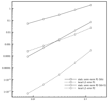
Figure 1: Left: convergence of global $L^{2}$-errors (dashed) and stabilization semi-norms (full). Right: convergence of local $L^{2}$-errors (dashed) and stabilization semi-norms (full). Square markers on curves representing $P_{1}$-approximation and circle markers on curves representing $P_{2}$-approximation.

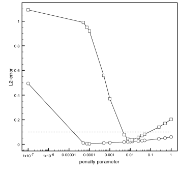
Figure 2: Study of the error under variation of the parameter $\gamma_{V}=\gamma_{W}$. ($P_{1}$ approximation marked with squares, $P_{2}$ with circles).

6 Conclusion and further perspecitives

Herein we have proposed a framework for the analysis of the stabilized methods introduced [2] when applied to ill-posed problems. The upshot is that error estimates can be obtained using only continuous dependence properties, without relying on a well-posedness theory of the continuous problem. Important extensions of the results presented herein are the inclusion of perturbed data and the exploration of the consequences of adjoint consistency. The latter may allow for improved estimates, when the error is measured by linear functionals that are in the range of the adjoint problem.

References

• [1] G. Alessandrini, L. Rondi, E. Rosset, and S. Vessella. The stability for the Cauchy problem for elliptic equations. Inverse Problems, 25(12):123004, 47, 2009.
• [2] E. Burman. Stabilized finite element methods for nonsymmetric, noncoercive, and ill-posed problems. Part I: Elliptic equations. SIAM J. Sci. Comput., 35(6): 2752– 2780, 2013.