Why are the magnetic field directions measured by Voyager 1 on both sides of the heliopause so similar?

Abstract

The solar wind carves in the interstellar plasma a cavity bounded by a surface, called the heliopause (HP), that separates the plasma and magnetic field of solar origin from the interstellar ones. It is now generally accepted that in August 2012 Voyager 1 (V1) crossed that boundary. Unexpectedly, the magnetic fields on both its sides, although theoretically independent of each other, were found to be similar in direction. This delayed the identification of the boundary as the heliopause and led to many alternative explanations. Here we show that the Voyager 1 observations can be readily explained and, after the Interstellar Boundary Explorer (IBEX) discovery of the ribbon, could even have been predicted. Our explanation relies on the fact that the Voyager 1 and the undisturbed interstellar field directions (which we assume to be given by the IBEX ribbon center (RC)) share the same heliolatitude ($\sim$34.5°) and are not far separated in longitude (difference $\sim$27°). Our result confirms that Voyager 1 has indeed crossed the heliopause and offers the first independent confirmation that the IBEX ribbon center is in fact the direction of the undisturbed interstellar magnetic field. For Voyager 2 we predict that the difference between the inner and the outer magnetic field directions at the heliopause will be significantly larger than the one observed by Voyager 1 ($\sim$30°  instead of $\sim$20°), and that the outer field direction will be close to the RC.

1 Introduction

In August 2012, V1 crossed the HP and entered the local interstellar medium (LISM) (Burlaga, Ness & Stone, 2013; Stone et al., 2013). Contrary to expectations, the change in the magnetic field direction across the HP was small (Burlaga, Ness & Stone, 2013) ($\sim$20°). As a result, the identification of the boundary as the HP remained in doubt. This led to speculations about the existence of an unexpected transition layer at the HP that allows enhanced exchange of energetic particles with the interstellar medium while conserving magnetic field characteristics typical for the heliosheath (Fisk & Gloeckler, 2013; Florinski, 2013; McComas & Schwadron, 2012; Stone et al., 2013; Schwadron & McComas, 2013). Only detection of electron plasma oscillations which allowed to evaluate the local plasma density at V1 in 2013, with values characteristic of the LISM, provided a strong evidence that the spacecraft has already crossed the heliopause (Gurnett et al., 2013). However it is still not understood why the magnetic field direction observed beyond the HP is so close to the field measured in the inner heliosheath, and attempts are still being made to answer this question (Schwadron & McComas, 2013; Fisk & Gloeckler, 2013; Florinski, 2013; Opher & Drake, 2013; Borovikov & Pogorelov, 2014).

In this letter we show how this observation can be explained in a simple and natural way if the undisturbed interstellar magnetic field (ISMF) far from the heliosphere points to the IBEX RC (Funsten et al., 2009). The ribbon is an almost circular arc in the sky of enhanced energetic neutral atoms emission discovered by the Interstellar Boundary Explorer (IBEX) (McComas et al., 2009; Funsten et al., 2009). The RC is widely interpreted as the direction of the undisturbed ISMF (Funsten et al., 2009; McComas et al., 2013; Funsten et al., 2013). We use the RC location given by Funsten et al. (2009) and McComas et al. (2009) (see Table 1). The recent energy averaged RC position (Funsten et al., 2013) differs from it only by 1.6°. A change by this amount would not affect our results significantly.

There are two crucial ingredients of our explanation. First, the heliolatitudes of V1 and the undisturbed ISMF happen to be approximately the same ($\sim$34.5°, see Table 1), with small angular distance between the two directions ($\sim$27°). Second, for a strong interstellar field, the draping around the HP has a simple structure, the evolution of which (in the region of HP not far from the undisturbed field direction) can be traced for the field magnitude decreasing towards the realistic values.

The essence of our argument is presented in Figure 1. The V1 and ISMF (RC) directions are shown on a sky map in orthogonal projection and Sun-centered equatorial (heliographic inertial) coordinates. From V1 observations we know (Burlaga, Ness & Stone, 2013) that the magnetic field on the inner side of the HP is very close to the Parker spiral, that is to the -T direction in the RTN system. Projected on the sky map, the solar magnetic field line is tangent to the heliographic parallel passing through the V1 position. B_IN and B_OUT denote the directions of the magnetic field measured by V1 before and after the crossing the HP, respectively.

The projection of the ISMF line passing through V1 position must link this point with the direction of the unperturbed ISMF (RC). If the draping pattern is such that the projected ISMF line reaches RC from V1 with little change in direction, the ISMF at V1 must be approximately parallel to the inner field simply because V1 and RC have the same heliolatitude.

2 Simple Draping Model

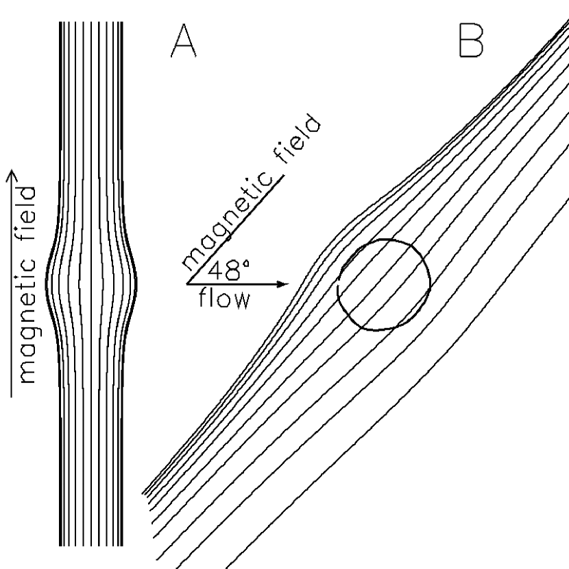
Figure 2: Draped interstellar magnetic field lines: A) in Parker’s solution (star at rest relative to the interstellar medium with insignificant plasma density), and B) obtained from 3DMHD simulations for spherically-symmetric solar wind and interstellar magnetic field of 20$\mu$G, inclined 48° to interstellar plasma flow (projection on a plane which contains interstellar flow and field vectors).

The simplest (’idealized’) draping model with this property is illustrated in Figure 1, where the selected draped ISMF field lines are shown as thick blue lines. We chose one of them to pass through the V1 and another through V2 position. In this model, based on the well-known solution by Parker (Parker, 1961) (see also Figure 2), the projected lines are arcs of great circles and originate in the undisturbed ISMF direction (RC).

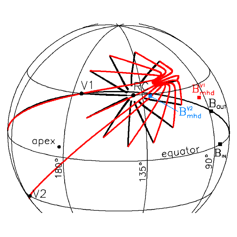
Figure 3: Comparison of draped interstellar magnetic field lines from our simulations for field strengths of 20 and 3 $\mu$G (black and red, respectively). The lines originate from selected points just outside the heliopause, distributed over a circle of radius 27° with the same center as the IBEX ribbon.

In Parker’s solution the star is at rest relative to the interstellar medium with insignificant plasma density and strong magnetic field. The stellar wind plasma flows away from the star, forming two streams, parallel and anti-parallel to the ISMF direction. Below we shall show, from our 3DMHD simulations (Czechowski et al., 2013), that the same idealized draping model can be regarded as the high ISMF strength limit for the case of the Sun, which is moving through the medium including the magnetized plasma. Moreover, when the ISMF strength is decreased to values actually observed by V1 beyond the HP (4-6 $\mu$G) (Burlaga et al., 2013), or, since the draped field near the HP can be stronger than the undisturbed ISMF (by $\sim{40}$% if the field is as weak as $\sim$3$\mu$G), even to lower values (3 $\mu$G or 2.7 $\mu$G, Grygorczuk et al. (2011); Heerikhuisen et al. (2014); BenJaffel et al. (2013)), the draped field near V1 direction in our heliographic projection remains similar enough in structure to the idealized model (Fig. 3) to agree approximately with V1 observations. The red line in Figure 1 shows the draped field line obtained for the ISMF of 4 $\mu$G. The angle between the red line and the heliographic parallel passing through V1 direction is larger than for the idealized draping model (the blue line). However, this is consistent with V1 observations, which correspond to the small but nonzero angle between the field outside and inside HP.

To agree with the V1 measurements, the red line at V1 position should be strictly tangent not to the heliographic parallel, but to the (V1, B_OUT) plane (defined by the V1 direction and the direction of the magnetic field measured by V1 outside the HP). In our projection this plane is represented by the great circle passing through the points V1 and B_OUT. Figure 1 shows that the draped field line corresponding to our draping model for the ISMF strength of 4 $\mu$G is indeed close to being tangent to this great circle. Moreover, the draped field direction in space derived from the model B${}^{V1}_{mhd}$ (the red square) is close ($\sim$10°) to the measured field direction B_OUT (the black square).

Figure 1 also shows the heliographic parallel and the magnetic field line for the idealized draping model, passing through the V2 position. The angle between the field line and the parallel is clearly large (30°) implying that the solar magnetic field and the draped ISMF will not be close in direction along the V2 trajectory. Similar values ($\sim$ 32° and 31°) are obtained in our 3DMHD simulations for the ISMF strength of 4 and 3 $\mu$G, respectively. The angular distance between V2 position and the RC is also much larger ($\sim$97°) than for V1.

The vicinity of the V1 direction is not the only region where the magnetic fields outside and inside the HP can be parallel (or antiparallel) to each other. In the idealized draping model, each of the interstellar magnetic field lines become tangent to a heliographic parallel at two points. The dashed blue line in Figure 1 shows a locus of such points situated between the north pole and ISMF directions (a similar line appears in the southern hemisphere). The draped field line which crosses this oval becomes tangent to the heliographic parallel at the crossing point (as illustrated by the elongated blue line in the north). If a spacecraft trajectory direction would be close to this line, then, assuming the idealized draping model, the solar and the interstellar fields observed at the heliopause would be approximately parallel (or antiparallel, for opposite polarity of the solar field). The actual direction of Voyager 1 trajectory (at the same solar latitude and close in longitude to the RC) satisfies this condition.

3 MHD Models

3DMHD simulations for the case of a star moving through a strongly magnetized (up to 20 $\mu$G) interstellar medium including also the plasma and neutral gas components (Czechowski et al., 2013) led to a two-stream structure of the stellar plasma flow. In this case the streams (containing most of the plasma flow) are slightly deflected from the interstellar field direction. The rest of the outflowing stellar plasma forms a tail opposite to the stellar motion. The two stream structure becomes less pronounced for larger values of the neutral interstellar hydrogen density. Nevertheless, the draping structure for the strong interstellar field case (Fig. 3, black arcs) remains similar to our simple draping model (Fig. 1, blue lines).

After the crossing of the HP, V1 is observing the interstellar field strength between 4 and 6 $\mu$G. To check the draping structure for the ISMF in this range we performed 3DMHD simulation for the local field strengths of 6, 5, 4, 3, and 2.7 $\mu$G, with the asymptotic field directed towards the IBEX RC. We found that the weaker the field the more its draping structure differs from the one of the strong (20 $\mu$G) field case. Figure 3 illustrates this difference for the ISMF strength of 3 $\mu$G. Although the draped field is not as simple as for the 20 $\mu$G, in our region of interest (between the undisturbed field (RC) and V1 direction) its structure simplifies and takes the form consistent with V1 magnetic field measurements. As explained above, the draped magnetic field line passing through the V1 trajectory is close to tangent to the plane defined by the V1 and B_OUT directions, and close in direction to the solar magnetic field on the inner side of the HP.

The direction of the draped magnetic field in space at the V1 position following from our models depends on the assumed ISMF strength. For a very strong field (20 $\mu$G) it is different from the V1 result B_OUT, but for the weaker and more realistic ISMF strength values it becomes close to B_OUT (within about 10°). At the same time, the angle between the draped magnetic field at V1 and the heliographic parallel increases from a low value (less than 10°) obtained for the idealized draping model and for strong ISMF (20 $\mu$G) to a somewhat higher value (15°, close to V1 observations) for the realistic ISMF.

In our calculations we use 3DMHD time-stationary numerical code describing the interaction of the solar wind with the LISM (boundary conditions for our models are shown in Table 2). The parameters of the solar wind are based on Ulysses data (Ebert et al., 2009). The interstellar medium parameters were chosen to agree with observations from the IBEX and Voyager 1 spacecraft (Gurnett et al., 2013), and model estimations. The code employs a fixed grid. A uniform flux of neutral hydrogen is assumed (Bzowski et al., 2009; Ratkiewicz & Grygorczuk, 2008). The solar magnetic field is disregarded to limit the undesired numerical effects (like artificial diffusion of the magnetic field at the HP) that could affect the heliopause region. In effect we assume that, as in ideal MHD case, there is no coupling between the magnetic fields across the HP.

We use the models to obtain the shape of the HP and the structure of the draped magnetic field. Since the HP in our models is not a discontinuity but a transition of finite width, we cannot reliably calculate the behaviour of quantities like the magnetic field strength or plasma density with distance in vicinity of the HP. For the magnetic field direction we find that the agreement of the 4 $\mu$G and 3 $\mu$G cases with V1 observations is satisfactory. The calculated ISMF direction at V1 just outside the HP (the red squares marked B${}^{V1}_{\rm mhd}$ in Figure 1 and Figure 3) are deflected by $\sim$ 11^o from the observed direction. While the distance to the HP is overestimated, the obtained termination shock distances at V1 and V2 are within few percent from the measured ones (Stone et al., 2005, 2008) when the slow wind speed is taken to be 500 km/s, but smaller (by less than 20 % for the slow wind speed of 400 km/s.

4 Discussion and Conclusions

Throughout this paper we are using the heliographic projection. We are interested in the magnetic field lines near the heliopause. The inner and the outer magnetic fields are then draped over the same surface. Since the heliopause is not strictly perpendicular to the radial direction, the angles between the projected field lines are not the same as the angles between the field lines in space. However, as long as we exclude the case of a heliopause tangent to the radial direction, the lines draped over the same element of the heliopause and strictly parallel (antiparallel) in projection have the same property also in space. We can therefore restrict attention to the heliographic projection and do not have to specify the shape of the actual heliopause. If the considered part of the heliopause is not very far from being perpendicular to radial direction, the field lines forming a small angle in projection, will also form a small angle in space.

Our results clarify the cause of similar magnetic field directions on both sides of the HP, as observed by V1: the heliographic latitude of V1 happens to be the same as that of the undisturbed ISMF (to be given by the IBEX RC). We have shown that for the wide range of the ISMF strength of values, including those actually observed by V1 beyond the HP, the draped interstellar field near V1 trajectory (calculated with zero heliospheric magnetic field to avoid artificial field diffusion across the boundary) must then be close in direction to the solar inner heliosheath magnetic field. For realistic ISMF strength values, our model results obtained for the draped field direction in space are within 10° from V1 observations beyond the HP. For Voyager 2 we predict that the difference between the inner and the outer magnetic field directions at the heliopause will be significantly larger than the one observed by Voyager 1 ($\sim$30° instead of $\sim$20°) and that the outer field direction will be close (7° - 9° off) to the RC.

The explanation is natural and simple, and removes the only objection against the claim that V1 reached the interstellar medium. It supports the interpretation of the ribbon center as the direction of the undisturbed ISMF, with the ISMF oriented towards the northern hemisphere It is consistent with the classical picture of the HP not dominated by the turbulence or reconnection effects. The reasonable agreement between V1 and our results for the magnetic field direction gives us confidence that the results are not affected by the approximations inherent to our models.

Approximate agreement with V1 magnetic field measurements was also achieved in numerical models that differ significantly from our approach. Borovikov & Pogorelov (2014) (see also Pogorelov et al. (2009)), who take HP instability into account, obtain a solution in which V1 is moving through a local interstellar plasma intrusion, partly surrounded by the heliosheath plasma. They predict that V1 may re-enter the heliosheath in the near future. Opher & Drake (2013), from numerical calculations that include both solar and interstellar magnetic fields, conclude that the presence of solar magnetic field strongly affects the draping of the ISMF over the HP. In their solution, for different asumptions about the undisturbed ISMF, the draped ISMF is close in direction to the heliospheric magnetic field in a large area of the HP including also the V1 and V2 trajectory directions. Calculations of Borovikov & Pogorelov (2014) do not confirm this result. The solar field assumed by Opher & Drake (2013) is very simplified. In particular, the sector polarity structure is ignored. Contrary to Opher & Drake (2013), we assume that the solar magnetic field does not strongly affect the shape of the HP and the draping pattern. The similarity of the field directions on both sides of the HP follows from the relative directions of V1 and the undisturbed ISMF.

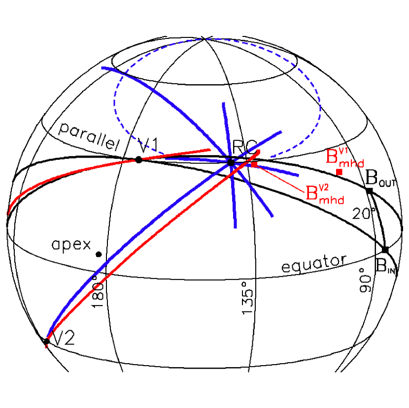
Figure 1: Sky map in orthogonal projection and heliographic inertial coordinates. Shown are: Voyager 1 (V1), Voyager 2 (V2), IBEX ribbon center (RC), interstellar inflow direction (apex), magnetic field directions measured by V1 before and after crossing the heliopause (B_IN and B_OUT, respectively). Two great circles (black) link V1 with B_OUT and B_IN (the latter is tangent to the heliographic parallel at V1). Thick blue lines are the interstellar magnetic field lines in the idealized draping model. The dashed blue oval is a locus of points where the idealized draped interstellar field lines become tangent to the local heliographic parallel (illustrated by the extended field line in the north). The thick red lines are the draped magnetic field lines obtained from our simulation for 4$\mu$G case. The red squares (B${}^{V1}_{mhd}$ and B${}^{V2}_{mhd}$) are the directions of the interstellar field just outside the heliopause at directions of V1 and V2 for the same simulation.

Table 1: Characteristic directions in galactic (GAL), solar ecliptic (SE), solar equatorial (HGI), and RTN coordinates (J2000).

	GAL		SE		HGI		RTN
	lon	lat	lon	lat	lon	lat	lon	lat
	(deg)	(deg)	(deg)	(deg)	(deg)	(deg)	(deg)	(deg)
$\rm V1$	32.7	28.1	254.9	35.0	174.1	34.5
$\rm V2$	342.1	-31.2	289.4	-34.2	217.2	-30.0
$\rm RC(=B_{\rm IS})$	32.9	55.3	221.0	39.0	140.9	34.6
$\rm apex$	5.3	12.0	259.0	4.98	182.6	5.4
$\rm B_{\rm IN}$	232.0	60.4	159.6	7.2	83.9	0.0	270.	0.
$\rm B_{\rm OUT}$	197.2	75.1	163.7	26.0	88.0	18.8	284.	13.
$B^{\rm V1}_{\rm MHD}\ \ 2.7\mu$G	155.	80.	169.	35.	93.	28.	293.	18.
$B^{\rm V1}_{\rm MHD}\ \ 3\mu$G	164.	73.	161.	35.	95.	28.	295.	17.
$B^{\rm V1}_{\rm MHD}\ \ 4\mu$G	168.	53.	137.	34.	100.	27.	298.	13.
$B^{\rm V1}_{\rm MHD}\ \ 20.0\mu$G	28.	63.	211.	36.	132.	31.	325.	3.
$B^{\rm V1}_{\rm MHD}\ \ 3\mu$G	159.	71.	159.	37.	93.	30.	294.	19.
$B^{\rm V1}_{\rm MHD}\ \ 4\mu$G	126.	83.	176.	36.	99.	29.	299.	16.
$\rm B^{\rm V2}_{\rm MHD}\ \ 2.7\mu$G	36.	65.	208.	39.	129.	34.	253.	29.
$\rm B^{\rm V2}_{\rm MHD}\ \ 3\mu$G	35.	64.	209.	39.	130.	33.	254.	30.
$\rm B^{\rm V2}_{\rm MHD}\ \ 4\mu$G	34.	62.	212.	39.	132.	34.	256.	31.
$B^{\rm V2}_{\rm MHD}\ \ 20.0\mu$G	30.	53.	224.	37.	143.	33.	265.	36.
$\rm B^{\rm V2}_{\rm MHD}\ \ 3\mu$G	37.	62.	212.	40.	133.	35.	255.	32.
$\rm B^{\rm V2}_{\rm MHD}\ \ 4\mu$G	35.	60.	215.	40.	135.	35.	257.	33.

• http://omniweb.gsfc.nasa.gov/coho/helios/coor_des.html

• http://www.srl.caltech.edu/ACE/ASC/coordinate_systems.html

• Table 2 solar wind case 400/750.

• Table 2 solar wind case 500/750.

Table 2: Boundary conditions for MHD calculations

LISM parameters					Solar Wind parameters
$\rm B_{\rm IS}$	$\rm T_{IS}$	$\rm n_{IS}$	$\rm n_{H}$	$\rm V_{IS}$	$\rm V_{SW,1AU}$	$\rm n_{SW,1AU}$
($\rm\mu$G)	(K)	(cm-3)	(cm-3)	(km/s)	(km/s)	(cm-3)
					slow/fast	slow/fast
20	6300	0.04	0.1	23.2	750	4.2
4, 5, 6	6300	0.06	0.1	23.2	400	5.55
2.7, 3, 4, 5	6300	0.06	0.1	23.2	400/750	5.55/1.58
3, 4	6300	0.06	0.1	23.2	500/750	5.55/2.46

• The inner boundary of the calculation region is at 15 AU, the outer at 5849 AU from the Sun.

• In the slow/fast solar wind cases, the slow wind flows within 36° from the solar equator.

References

- BenJaffel et al. (2013) BenJaffel, L., Strumik, M., Ratkiewicz, R. & Grygorczuk, J. 2013, ApJ, 779, 130
- Borovikov & Pogorelov (2014) Borovikov, S. N., & Pogorelov, N. V. 2014, ApJ, 783, L16
- Burlaga, Ness & Stone (2013) Burlaga, L. F., Ness, N. F., & Stone, E.C. 2013, Science, 341, 147
- Burlaga et al. (2013) Burlaga, L. F., Ness, N. F., Gurnett, D. A., & Kurth, W. S. 2013, ApJ, 778, L13
- Bzowski et al. (2009) Bzowski, M., Moebius, E., Tarnopolski, S., Izmodenov, V., Gloeckler, G. 2009, Space Sci. Rev., 143, 177
- Czechowski et al. (2013) Czechowski, A., Grygorczuk, J., McComas, D., & Ratkiewicz, R. 2013, A&A, submitted
- Ebert et al. (2009) Ebert, R. W., McComas, D. J., Elliott, H. A., Forsyth, R. J., & Gosling, J. T. 2009, J. Geophys. Res., 114, 1109
- Fisk & Gloeckler (2013) Fisk, L. A. & Gloeckler, G. 2013, ApJ, 776, 79
- Florinski (2013) Florinski V. 2013, arXiv:1302.2179v1
- Franz & Harper (2002) Franz, M., & Harper, D. 2003, Planetary & Space Science, 50, 217-233
- Funsten et al. (2009) Funsten, H. O., Allegrini, F., Crew, G. B., DeMajistre, R., Frisch, P. C., et al. 2009, Science, 326, 964
- Funsten et al. (2013) Funsten, H. O., De Majistre, R., Frisch, P. C., Heerikhuisen, J., Higdon, D. M., Janzen, P., Larsen, B. A., Livadiotis, G., McComas, D. J., Moebius, E., Reese, C. S., Reisenfeld, D. B., Schwadron, N. A., & Zirnstein, E. J. 2013, ApJ, 776, 30
- Grygorczuk et al. (2011) Grygorczuk, J., Ratkiewicz, R., Strumik, M. & Grzedzielski, S. 2011, ApJ, 727, L48
- Gurnett et al. (2013) Gurnett, D. A., Kurth, W. S., Burlaga, L. F., and Ness, N. F. 2013, ApJ, 341, 1492
- Heerikhuisen et al. (2014) Heerikhuisen, J., Zirnstein, E. J., Funsten, H. O., Pogorelov, N. V., & Zank, G. P. 2014, ApJ, 784, 73
- McComas & Schwadron (2012) McComas, D. J. & Schwadron, N. A. 2013, ApJ, 758, 19
- McComas et al. (2009) McComas D. J.,Allegrini, F., Bochsler, P., Bzowski, M., Christian, E. R., et al. 2009, Science, 326, 13
- McComas et al. (2013) McComas, D.J., Dayeh,M.A., Funsten, H. O., Livadiotis, G., & Schwadron, N. A. 2013, ApJ, 771, 77
- Opher & Drake (2013) Opher, M., & Drake, J. F. 2013, ApJ, 778, L26
- Parker (1961) Parker, E. N. 1961, ApJ, 134, 20-27
- Pogorelov et al. (2009) Pogorelov, N. V., Borovikov, S. N., Zank, G. P., & Ogino, T. 2009, ApJ, 696, 1478-1490
- Ratkiewicz & Grygorczuk (2008) Ratkiewicz, R., & Grygorczuk, J. 2008, Geophys. Res. Lett., 35, L23105
- Schwadron & McComas (2013) Schwadron, N. A. & McComas, D. J. 2013, ApJ, 778, L33 9
- Stone et al. (2005) Stone, E. C., Clummings, A. C., McDonald, F. B., Heikkila, B. C., Lal, N., & Webber, W. R. 2005, Science, 309, 2017
- Stone et al. (2008) Stone, E. C., Clummings, A. C., McDonald, F. B., Heikkila, B. C., Lal, N., & Webber, W. R. 2008, Nature, 454, 71
- Stone et al. (2013) Stone, E. C., Cummings, A. C., McDonald, F. B., Heikkila, B. C., Lal, N., & Webber, W. R. 2013, Science, 341, 150