Mass scaling and non-adiabatic effects in photoassociation spectroscopy of ultracold strontium atoms

Abstract

We report photoassociation spectroscopy of ultracold ⁸⁶Sr atoms near the intercombination line and provide theoretical models to describe the obtained bound state energies. We show that using only the molecular states correlating with the ${}^{1}S_{0}$$+$${}^{3}P_{1}$ asymptote is insufficient to provide a mass scaled theoretical model that would reproduce the bound state energies for all isotopes investigated to date: ⁸⁴Sr, ⁸⁶Sr and ⁸⁸Sr. We attribute that to the recently discovered avoided crossing between the ${}^{1}S_{0}$$+$${}^{3}P_{1}$ $0_{u}^{+}$ (${}^{3}\Pi_{u}$) and ${}^{1}S_{0}$$+$${}^{1}D_{2}$ $0_{u}^{+}$ (${}^{1}\Sigma^{+}_{u}$) potential curves at short range and we build a mass scaled interaction model that quantitatively reproduces the available $0_{u}^{+}$ and $1_{u}$ bound state energies for the three stable bosonic isotopes. We also provide isotope-specific two-channel models that incorporate the rotational (Coriolis) mixing between the $0_{u}^{+}$ and $1_{u}$ curves which, while not mass scaled, are capable of quantitatively describing the vibrational splittings observed in experiment. We find that the use of state-of-the-art ab initio potential curves significantly improves the quantitative description of the Coriolis mixing between the two $-8$ GHz bound states in ⁸⁸Sr over the previously used model potentials. We show that one of the recently reported energy levels in ⁸⁴Sr does not follow the long range bound state series and theorize on the possible causes. Finally, we give the Coriolis mixing angles and linear Zeeman coefficients for all of the photoassociation lines. The long range van der Waals coefficients $C_{6}(0_{u}^{+})=3868(50)$ a.u. and $C_{6}(1_{u})=4085(50)$ a.u. are reported.

I Introduction

Photoassociation (PA) spectroscopy is a widely used tool for the study of atomic collisions and determination of bound state energies of diatomic molecules Jones et al. (2006). In this process two colliding cold atoms are bound together into an excited molecule by optical excitation. A recent focus for PA spectroscopy has been the study of molecules created by excitation to the red of an intercombination line (${}^{1}S_{0}$$\rightarrow$${}^{3}P_{1}$) in divalent atoms such as alkaline-earth metal atoms calcium Kahmann et al. (2014) and strontium Zelevinsky et al. (2006); McGuyer et al. (2013); Stellmer et al. (2012), and the rare-earth atom ytterbium Tojo et al. (2006); Borkowski et al. (2009, 2011); Takasu et al. (2012). The interest in intercombination line PA spectroscopy Ciuryło et al. (2004) is driven by its potential applications in the production of ground state ultracold molecules Skomorowski et al. (2012), the potential for control of scattering lengths in ultracold collisions via optical Feshbach resonances Ciuryło et al. (2005), as well as coherent photoassociation Koch and Shapiro (2012); Yan et al. (2013) and finally electron-proton mass ratio measurements Kotochigova et al. (2009).

The interactions between strontium atoms, both in their ground and excited states, have been extensively studied by means of intercombination line PA spectroscopy. Zelevinsky et al. Zelevinsky et al. (2006) made the first observations with ⁸⁸Sr atoms confined in an optical lattice and recently Stellmer et al. Stellmer et al. (2012) have reported similar measurements with ⁸⁴Sr atoms. Two-color photoassociation spectroscopy enabled Martinez de Escobar et al. Martinez de Escobar et al. (2008) to accurately determine the scattering lengths of all Sr isotopes which helped to explain the low thermalization rate in ⁸⁸Sr. In addition to the PA spectroscopy studies, both the interactions in the ground Stein et al. (2008, 2010) and excited Stein et al. (2011) states of the Sr₂ molecule have been studied by Fourier transform spectroscopy.

The research into intercombination line PA is fueled by the possible use of optical Feshbach resonances (OFRs) Fedichev et al. (1996); Bohn and Julienne (1997); Chin et al. (2010) to enable optical control of the scattering lengths. This is especially important for ground state strontium atoms, because its ${}^{1}S_{0}$ ground state and a lack of hyperfine structure in its bosonic isotopes precludes the existence of magnetic Feshbach resonances in this system. Early experiments with Na Lett et al. (1993); Fatemi et al. (2000) and Rb Theis et al. (2004); Thalhammer et al. (2005) have shown that the usefulness of OFRs in alkali-metals is greatly hindered by the large loss of atoms due to photoassociation. However, in the case of the narrow intercombination lines in divalent atoms like Ca, Sr, and Yb, these losses can be greatly reduced Ciuryło et al. (2004, 2005) and useful changes in scattering lengths have been shown for both Yb Enomoto et al. (2008) and recently Sr: a proof-of-concept investigation in a thermal gas Blatt et al. (2011) and an example of the use of OFRs as a means of controlling the collapse of an Sr Bose-Einstein condensate (BEC) Yan et al. (2013).

All isotopes of Sr have been brought to quantum degeneracy. The most abundant isotope ⁸⁸Sr is known for its small negative scattering length Mickelson et al. (2005); Martinez de Escobar et al. (2008), which thwarted the early attempts Ido et al. (2000); Ferrari et al. (2006) at quantum degeneracy. The least abundant isotope, ⁸⁴Sr, has excellent collision properties for evaporative cooling, so it was the first Bose-condensed isotope Stellmer et al. (2009); de Escobar et al. (2009). Since then, the isotope ⁸⁶Sr has also been condensed Stellmer et al. (2010), while the thermalization problem in ⁸⁸Sr has been circumvented by sympathetic cooling with ⁸⁷Sr Mickelson et al. (2010). The narrow intercombination line enabled direct laser cooling of ⁸⁴Sr down to quantum degeneracy Stellmer et al. (2013a). Degenerate Fermi DeSalvo et al. (2010) and Bose-Fermi gases Stellmer et al. (2013b) have also been reported. Strontium is being actively explored for its use in the making of ultracold molecules: ground state strontium dimers Skomorowski et al. (2012); Reinaudi et al. (2012), and the heteronuclear RbSr molecules Tomza et al. (2011). Rubidium-strontium mixtures have become especially promising after a degenerate quantum mixture of Rb and Sr atoms was obtained Pasquiou et al. (2013).

We report energy levels of the ¹S₀+³P₁ Sr₂ molecule obtained for the ⁸⁶Sr isotope, which complements the currently available data for ⁸⁸Sr Zelevinsky et al. (2006) and ⁸⁴Sr Stellmer et al. (2012), and we provide theoretical models of the interactions in the Sr₂ molecule. A set of energy levels in the subradiant $1_{g}$ state of the strontium dimer has also become available McGuyer et al. , but is outside the scope of this article. The paper is organized as follows. In Section II we briefly describe the experimental details and the PA data obtained for ⁸⁶Sr. In Section III we provide a theoretical model based on recent state-of-the-art ab initio potential curves Skomorowski et al. (2012) for the description of the long range interactions in this excited state of the strontium dimer. We will use this model in Section IV to provide a quantitative description of vibrational splittings, as well as the nonadiabatic Coriolis effects and linear Zeeman coefficients McGuyer et al. (2013) for all photoassociation lines reported to date. In the case of one of the isotopes, ⁸⁴Sr, we will find a significant discrepancy between one of the experimental Stellmer et al. (2012) and theoretical positions of one of the lines and theorize on its possible causes. In the case of ⁸⁸Sr we will show that the use of realistic potential curves significantly improves the quantitative description of the positions of strongly Coriolis-mixed energy levels over previous work Zelevinsky et al. (2006). We also show that the improvement of the description of Coriolis mixing is followed by better agreement of the respective Zeeman g-factors with the experimental data McGuyer et al. (2013). Finally, in Section VI we will investigate the mass scaling between strontium isotopes, that is, the possibility of using the same potential curves for the description of PA spectroscopy data for all isotopes. While mass scaling of only the long range potentials was sufficient in the description of the energy levels near the ¹S₀+³P₁ asymptote in different isotopes of a similar species ytterbium Borkowski et al. (2009), it fails in the case of strontium. We will explain this effect for the $0_{u}^{+}$ series quantitatively by augmenting our model with the recently discovered Stein et al. (2011); Skomorowski et al. (2012) curve crossing between the ¹S₀+³P₁ ${}^{3}\Pi_{u}$ curve (which supports the $0_{u}^{+}$ series) and a ${}^{1}\Sigma_{u}^{+}$ curve correlating, remarkably, to the ¹S₀+¹D₂ asymptote. Once mass-scaling of the $0_{u}^{+}$ bound states is achieved we add a third channel representing the ${}^{1}S_{0}$+${}^{3}P_{1}$ $1_{u}$ state. The final three-channel mass scaled model reproduces the available $0_{u}^{+}$ and $1_{u}$ bound state energies to within $0.5$ MHz on average.

II Photoassociation spectroscopy of ⁸⁶Sr

Table 1: Comparison of available experimental ${}^{1}S_{0}$$\rightarrow$${}^{3}P_{1}$ photoassociation data with our long range interaction model. The experimental data encompasses all bosonic isotopes: ⁸⁸Sr (for total angular momentum $J=1$ Zelevinsky et al. (2006), and recently $J=3$ McGuyer et al. (2013)), ⁸⁴Sr data from Stellmer et al. Stellmer et al. (2012), and the previously unreported data for ⁸⁶Sr. The numbers in parentheses denote the experimental uncertainty, where available. The model parameters were initially fitted to the bound state energies for ⁸⁸Sr and then extended to other isotopes by only changing the respective short range wavefunction phase. For ⁸⁸Sr we also cite the theoretical bound state energies from the original Zelevinsky et al. Zelevinsky et al. (2006) model to show the improved description of Coriolis mixing between the two bound states at -8430 and -8200 MHz that our model provides. For ⁸⁴Sr we find it difficult to fit all of the energy levels together, therefore the results shown are based on a fit that omits the $-1288$ MHz state. The observed drastic discrepancy between this state and the theoretical energy suggests that the $-1288$ MHz may not be a member of the $0_{u}^{+}$ $J=1$ series. This is discussed in Section IV. We also give the Coriolis mixing angles and Zeeman g-factors as measured in Ref. McGuyer et al. (2013) and their theoretical counterparts as described in Section V.

			Binding energy $E/h$ (MHz)			Mixing angle $\theta$		Linear Zeeman coefficient $g$
Isotope	Series	$J$	Exp. Zelevinsky et al. (2006)	Theory Zelevinsky et al. (2006)	Theory, this work	Theory McGuyer et al. (2013)	This work	Exp. McGuyer et al. (2013)	Theory McGuyer et al. (2013)	Theory, this work
88Sr	$0_{u}^{+}$	1	-0.435(37)	-0.418	-0.427	16.5∘	17.46∘	0.666(14)	0.636	0.659
	$0_{u}^{+}$	1	-23.932(33)	-23.932	-23.880	6.1∘	6.07∘	0.232(2)	0.222	0.228
	$0_{u}^{+}$	1	-222.161(35)	-222.162	-222.167	4.2∘	4.04∘	0.161(2)	0.148	0.147
	$1_{u}$	1	-353.236(35)	-353.236	-353.152	93.3∘	93.89∘	0.625(9)	0.610	0.612
	$0_{u}^{+}$	1	-1084.093(33)	-1084.092	-1084.022	3.8∘	3.59∘	0.142(2)	0.128	0.131
	$1_{u}$	1	-2683.722(32)	-2683.723	-2683.777	94.6∘	94.90∘	0.584(8)	0.571	0.577
	$0_{u}^{+}$	1	-3463.280(33)	-3463.281	-3463.346	5.1∘	4.88∘	0.193(3)	0.174	0.173
	$1_{u}$	1	-8200.163(39)	-8112.699	-8200.219	{113.6∘, 175.9∘}	112.58∘	-0.149(2)	-0.592	-0.024
	$0_{u}^{+}$	1	-8429.650(42)	-8420.133	-8427.888	{24.6∘, 84.9∘}	22.58∘	0.931(13)	1.333	0.774
Isotope	Series	$J$	Exp. McGuyer et al. (2013)		Theory, this work	Theory McGuyer et al. (2013)	This work	Exp. McGuyer et al. (2013)	Theory McGuyer et al. (2013)	Theory, this work
88Sr	$0_{u}^{+}$	3	-0.63		-0.644	18.9∘	18.92∘	0.270(2)	0.271	0.271
	$0_{u}^{+}$	3	-132		-134.217	11.6∘	12.22∘	0.173(2)	0.160	0.157
Isotope	Series	$J$	Exp., this work		Theory, this work		This work			Theory, this work
86Sr	$0_{u}^{+}$	1	-1.633(10)		-1.534		12.93∘			0.490
	$0_{u}^{+}$	1	-44.246(10)		-43.850		6.36∘			0.214
	$1_{u}$	1	-159.984(50)		-159.993		97.31∘			0.556
	$0_{u}^{+}$	1	-348.742(10)		-348.825		6.67∘			0.206
Isotope	Series	$J$	Exp. Stellmer et al. (2012)		Theory, this work		This work			Theory, this work
84Sr	$0_{u}^{+}$	1	-0.320(10)		-0.296		19.56∘			0.736
	$0_{u}^{+}$	1	-23.010(10)		-23.011		6.48∘			0.242
	$0_{u}^{+}$	1	-228.380(10)		-228.380		3.47∘			0.116
	$0_{u}^{+}$	1	-1288.290(10)		-1144.492		3.11∘			0.113 (0.101)

To perform photoassociation (PA), we prepare ultracold ⁸⁶Sr atoms in an optical dipole trap (ODT) via laser cooling and trapping techniques similar to those used for other Sr isotopes Nagel et al. (2003); Yan et al. (2011). The ODT is formed by the intersection of two mutually perpendicular beams focused to waists ($e^{-2}$ intensity radii) of 100 $\mu$m. Both beams are generated from a 1064-nm, linearly-polarized, multilongitudinal-mode fiber laser. A period of forced evaporation to a trap depth of 3.6 $\mu$K yields $3\times 10^{5}$ ⁸⁶Sr atoms at a temperature of 400 nK and peak density of $10^{13}$ cm^-3.

The PA beam is derived from a 689 nm master-slave diode laser system that has a linewidth of approximately 10 kHz. Short term stability is provided by locking the laser frequency to a moderate finesse ($\mathcal{F}=2000$) optical cavity, and long term stability is assured through saturated absorption spectroscopy of the ${}^{1}S_{0}$-${}^{3}P_{1}$ atomic transition in a vapor cell. The PA beam is red detuned with respect to the atomic transition using acousto-optic modulators (AOMs) and transported to the atoms through a single-mode optical fiber. In the interaction region, the beam is linearly polarized, with a waist of 700 $\mu$m and peak intensity up to 50 mW/cm². During the application of the PA beam, to eliminate the ac-Stark shift due to ODT beams, the ODT is modulated with 50% duty cycle, a period of 462 $\mu$s, and a peak trap depth of 7.2 $\mu$K. The PA beam is applied when the ODT is off. Total PA time is varied from 16 to 830 ms, depending upon the transition, to obtain a peak atom loss due to PA of approximately 50% with minimal change in sample temperature. The number of atoms and sample temperature are determined with time-of-flight absorption imaging using the ¹S₀-¹P₁ transition at 461 nm.

New ⁸⁶Sr photoassociation lines found in our experiment are listed in Table 1. The binding energies $\nu_{0}$ were obtained by fitting the trap loss spectra with a realistic line shape function Ciuryło et al. (2004). The details of this procedure, the error budget and the respective optical lengths are given in Appendix A.

III Long range interactions

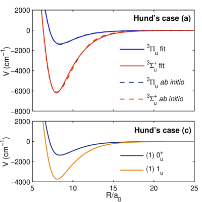
Figure 1: (Color online) Potential curves correlating to the ${}^{1}S_{0}$+${}^{3}P_{1}$ asymptote used in the calculation of the theoretical binding energies. The dashed curves represent the original ab initio Hund’s case (a) potentials of Skomorowski et al. Skomorowski et al. (2012). The solid lines are the potential curves fitted to the experimental data from photoassociation experiments. The top panel shows the potential curves in the Hund’s case (a) representation, while the bottom panel shows them in the Hund’s case (c) basis actually used in the calculation.

Table 2: Potential parameters used in the calculation of theoretical ${}^{1}S_{0}$+${}^{3}P_{1}$ bound state energies in Table 1. The potential parameters given here are to be used with Eq. 3. The only isotope-dependent parameter is $\alpha$, which is used to establish the correct short range quantum defect for each curve.

Parameter	${}^{3}\Sigma_{u}^{+}$	${}^{3}\Pi_{u}$
$A_{0}$	$1.29406314\times 10^{2}$	$5.78723038\times 10^{6}$
$A_{1}$	$-7.90551852\times 10^{1}$	$-3.46113235\times 10^{6}$
$A_{2}$	$1.87863441\times 10^{1}$	$7.79019763\times 10^{5}$
$A_{3}$	$-1.96979418\times 10^{0}$	$-7.85317879\times 10^{4}$
$A_{4}$	$7.88636443\times 10^{-2}$	$3.01833743\times 10^{3}$
$\gamma$	$7.61382806\times 10^{-2}$	$1.34967817\times 10^{-3}$
$\beta$	$1.00$	$1.03238202$
$\alpha(^{88}\rm{Sr})$	$0.045647282$	$1.99168225$
$\alpha(^{86}\rm{Sr})$	$0.045690735$	$1.99188286$
$\alpha(^{84}\rm{Sr})$	$0.045301189$	$1.99037413$
$C_{12}$	$-5.31841848\times 10^{9}$	$-1.06415514\times 10^{10}$
$C_{10}$	$2.20495\times 10^{8}$	$5.24064\times 10^{7}$
$C_{8}$	$2.3574797\times 10^{6}$	$3.4156471\times 10^{5}$
$C_{6}$	$4.3015063\times 10^{3}$	$3.8683912\times 10^{3}$
$C_{3,0}$	$1.52356615\times 10^{-2}$

In the original paper by Zelevinsky et al. Zelevinsky et al. (2006), the energy levels obtained for ⁸⁸Sr were modeled using a five channel model Ciuryło et al. (2004) which included both the relevant molecular states from the ¹S₀+³P₁ asymptote as well as ones from the ¹S₀+¹P₁ and ¹S₀+³P₂ asymptotes. The energy levels for ⁸⁸Sr reproduced by this model are shown in Table 1 (labeled ‘Theory Zelevinsky et al. (2006)’).

In this paper we will use a two-channel model based on the two long range Hund’s case (c) potential curves, $0_{u}^{+}$ and $1_{u}$, that directly support the vibrational states near the ${}^{1}S_{0}$+${}^{3}P_{1}$ asymptote. The molecular Hamiltonian can be partitioned in the following manner:

$$H=T+V_{\rm int}+V_{\rm rot}.$$ (1)

Here, $T$ is the kinetic energy of the colliding atoms, $V_{\rm int}$ covers the interaction potentials, while $V_{\rm rot}$ is the rotational energy of the molecule. The kinetic energy term is diagonal regardless of chosen basis, with the diagonal term $-({\hbar^{2}}/{2\mu})({d^{2}}/{dR^{2}})$. In our homonuclear case, the reduced mass $\mu$ is equal to half the atomic mass of the chosen strontium isotope.

In this paper we choose to work with potential curves based on state-of-the-art ab initio calculation of Skomorowski et al. Skomorowski et al. (2012) as opposed to using model potentials. Using the model in Mies et al. (1978) we can write a two-channel Hund’s case (c) atomic interaction hamiltonian in terms of Hund’s case (a) potential curves:

$$V_{\rm int}=\left(\begin{array}[]{c c}\mathcal{V}(^{3}\Pi_{u};R)-\frac{C_{3,0}}{R^{3}}&0\\ 0&\frac{1}{2}\left(\mathcal{V}(^{3}\Pi_{u};R)+\mathcal{V}(^{3}\Sigma^{+}_{u};R)\right)-\frac{C_{3,1}}{R^{3}}\end{array}\right)\,.$$ (2)

Our Hund case (a) potentials $\mathcal{V}(^{3}\Pi_{u},R)$ and $\mathcal{V}(^{3}\Sigma_{u}^{+},R)$ are based on the ab initio potentials in Skomorowski et al.: $\mathcal{V}(^{3}\Pi_{u},R)=\left(V({\rm c}~{}^{3}\Pi_{u};R)-V({\rm c}~{}^{3}\Pi_{u};\infty)\right)$ and $\mathcal{V}(^{3}\Sigma_{u}^{+},R)=V({\rm a}~{}^{3}\Sigma^{+}_{u};R)-V({\rm a}~{}^{3}\Sigma^{+}_{u};\infty)$, where $V({\rm c}~{}^{3}\Pi_{u};R)$ and $V({\rm a}~{}^{3}\Sigma^{+}_{u};R)$ are the respective potential curves. The original ab initio potential curves were given in the convenient form of a short range part combined with a Tang-Toennies damped Tang and Toennies (1984) long range part and enabled direct fitting of the potential parameters:

$$V(R)=e^{-\alpha R-\gamma R^{2}}\left(A_{0}+A_{1}R+A_{2}R^{2}+A_{3}R^{3}+A_{4}R^{4}\right)-$$

$$-C_{12}f_{12}R^{-12}-C_{10}f_{10}R^{-10}-C_{8}f_{8}R^{-8}-C_{6}f_{6}R^{-6}\,,$$ (3)

where $f_{n}(R)$ is a Tang-Toennies damping function of the $n$-th order Tang and Toennies (1984). During the fitting it was necessary to change the long range $C_{6}$ and $C_{8}$ terms significantly. In order to retain the shape of the potential curves we have refitted the remaining potential parameters to match the shape of the original ab initio potentials, as shown in Figure 1. The potential parameters used in our calculations are listed in Table 2. Finally, we have included the resonant dipole interaction King and van Vleck (1939) into the model. In Skomorowski et al. this was achieved by spin-orbit mixing between states correlating to the ${}^{1}S_{0}$$+$${}^{1}P_{1}$ and ${}^{1}S_{0}$$+$${}^{3}P_{1}$ asymptotes. Since, however, we do not expect any new physics emerging from the inclusion of the far ${}^{1}S_{0}$$+$${}^{1}P_{1}$ asymptote, we decide to model this mixing by simply adding the dipole terms artificially, following Mies et al. (1978). In this case these terms are inversely proportional to the lifetime of the ${}^{3}P_{1}$ atomic state in strontium:

$$C_{3,0}=\frac{3}{2}\frac{\hbar}{\tau}\left(\frac{\lambda}{2\pi}\right)^{3}\,,$$ (4)

and

$$C_{3,1}=-C_{3,0}/2\,.$$ (5)

The resonant dipole interaction is thus attractive in the $0_{u}^{+}$ curve while repulsive (and weaker) in the $1_{u}$ state.

The remaining term in the molecular Hamiltonian is the rotational energy $V_{\rm rot}$, which is diagonal in the Hund’s case (e), but not in the Hund’s case (c) representation. This causes rotational (Coriolis) mixing between the two molecular states:

$$V_{\rm rot}=B(R)\left(\begin{array}[]{c c}J(J+1)+2&-\sqrt{4J(J+1)}\\ -\sqrt{4J(J+1)}&J(J+1)\\ \end{array}\right)$$ (6)

with $B(R)={\hbar^{2}}/{2\mu R^{2}}$. In a similar study with ytterbium atoms Borkowski et al. (2009) the large dispersion between the two potentials caused by the differences in the resonant dipole interaction (see eq.(5)) made it possible to forego Coriolis mixing and fit the available energy level data with a single channel potential. Here, however, the dipole interaction is much weaker, making it necessary to include this mixing in order to properly recreate bound state energies very close to the dissociation limit. Not including the Coriolis mixing limits the accuracy of the model to about $1$ MHz for most energy levels. The exception to this rule is the case of strongly mixed states, like the $-8200$ MHz and $-8430$ MHz states in ⁸⁸Sr, where this inaccuracy is drastic, as shown in Section IV.

Theoretical bound state energies can be obtained by solving the coupled channel Schrödinger equation $H\Psi=E\Psi$, where $\Psi=\left(\Psi(0_{u}^{+};R),\,\Psi(1_{u};R)\right)^{T}$ is the two-channel wavefunction. We solve these equations numerically using the matrix DVR method Tiesinga et al. (1998) with nonlinear coordinate scaling.

The long range parameters of the Hund’s case (a) potentials $V({\rm a}~{}^{3}\Sigma_{u}^{+};R)$ and $V({\rm c}~{}^{3}\Pi_{u};R)$ were fitted to the experimental data using the nonlinear least-squares method. The long range resonant dipole $C_{3}$, the two van der Waals terms $C_{6}({\rm a}~{}^{3}\Sigma_{u}^{+})$ and $C_{6}({\rm c}~{}^{3}\Pi_{u})$ and the two respective $C_{8}$ terms were first used to match the vibrational energies only for the $J=1$ ⁸⁸Sr data. To a good approximation, the $C_{3}$ and $C_{6}$ (and to a lesser extent $C_{8}$) coefficients determine the vibrational splittings. Here, the short range $\alpha$ terms can be used to tune the phases (or ‘quantum defects’) of the short range parts of the radial wavefunctions and effectively shift the whole vibrational series in place. This parameter was chosen for phase adjustments in an attempt to preserve the shape of the short range potential as much as possible. The resulting bound state energies can be seen in Table 1. The energy levels for $J=3$ were computed using the same set of parameters.

Table 3: Van der Waals coefficients $C_{6}$ for Sr₂ molecular states correlating to the ${}^{1}S_{0}$+${}^{3}P_{1}$ asymptote given in Hund’s case (a) and (c) bases.

Source	$C_{6}({}^{3}\Pi_{u})$	$C_{6}({}^{3}\Sigma_{u}^{+})$	$C_{6}(0_{u}^{+})$	$C_{6}(1_{u})$
Empirical Zelevinsky et al. (2006)	$3513\pm 200$	$4035\pm 600$	$3513\pm 200$	$3774\pm 200$
Ab initio Mitroy and Zhang (2010)	$3951$	$4488$	$3951$	$4220$
Ab initio
(pure) Porsev et al. (2014)	3821	4289	3821	4055
Ab initio
(recomm.) Porsev et al. (2014)	$3771\pm 32$	$4231\pm 98$	$3771\pm 32$	$4001\pm 33$
This work	$3868\pm 50$	$4302\pm 150$	$3868\pm 50$	$4085\pm 50$

The vibrational level data for the remaining two isotopes, ⁸⁶Sr and ⁸⁴Sr was modeled by adjusting only the two $\alpha$ coefficients on a per isotope basis in order to fix the right short range wavefunction phase. The differences between the $\alpha$ coefficients for different isotopes do not exceed $1\%$. Therefore, the theoretical bound state energies listed in the ‘Theory (this work)’ of Table 1 were calculated using slightly different potential curves that shared the same set of the van der Waals $C_{6}$ and $C_{8}$ coefficients: $C_{6}(~{}^{3}\Sigma_{u}^{+})\approx 4302~{}{\rm a.u.}$ and $C_{6}(^{3}\Pi_{u})\approx 3868~{}{\rm a.u.}$, which correspond to $C_{6}(0_{u}^{+})=3868~{}{\rm a.u.}$ and $C_{6}(1_{u})=4085~{}{\rm a.u.}$ in the Hund’s case (c) representation. The $C_{8}$ coefficients are $C_{8}(^{3}\Sigma_{u}^{+})\approx 2.36\times 10^{6}$ a.u. and $C_{8}(^{3}\Pi_{u})\approx 3.42\times 10^{5}$ a.u.. We tentatively assign an error bound of $50~{}{\rm a.u.}$ to each of the Hund’s case (c) $C_{6}$ coefficients: a change of this size introduces a change in the vibrational splittings that can not be compensated using the other long range parameters. We choose to assign uncertainties to the Hund’s case (c) parameters because those directly affect the positions of the photoassociation resonances. In the Hund’s case (a) representation this results in uncertainties of 50 a.u. and 150 a.u. for $C_{6}(^{3}\Pi_{u})$ and $C_{6}(^{3}\Sigma_{u}^{+})$ assuming our estimations should be treated as maximum errors. Our fitted resonant dipole term $C_{3,0}\approx 0.01524~{}{\rm a.u.}$ which corresponds to a natural linewidth of the atomic ${}^{3}P_{1}$ state of $1/\tau=2\pi\times 7501.9$ Hz. Our lifetime of $21.215~{}\mu$s agrees well with both the theoretical determination Skomorowski et al. (2012) of $21.4~{}\mu$s and, not surprisingly, the empirical value of $21.5~{}\mu$s from the previous photoassociation experiment Zelevinsky et al. (2006).

Our $C_{6}$ coefficients can be compared to previous works (see Table 3). The first photoassociation-based determination Zelevinsky et al. (2006) gives $C_{6}(0_{u}^{+})=3513~{}{\rm a.u.}$ and $C_{6}(1_{u})=3774$ a.u., respectively with an estimated error bound of $200$ a.u. These values appear to be underestimated when compared to both our work and the recent ab initio determinations. The Hund’s case (a) $C_{6}$ values originally calculated by Mitroy and Zhang Mitroy and Zhang (2010) and used in the model in Skomorowski et al. are $4488$ a.u. and $3951$ a.u. for the respective ${}^{3}\Sigma_{u}^{+}$ and ${}^{3}\Pi_{u}$ states, which is about one and a half error bound larger than our empirical determination. We note, however, that no error bound was given for their calculation. A new ab initio calculation by Safronova et al. Porsev et al. (2014) is also available. The first set of coefficients, $C_{6}(0_{u}^{+})=3821$ a.u. and $C_{6}(1_{u})=4055$ a.u. is of pure ab initio origin (labeled ‘Ab initio (pure) Porsev et al. (2014)’ in Table 3) and fits our data perfectly. The second set of coefficients (‘Ab initio (recomm.) Porsev et al. (2014)’), $C_{6}(0_{u}^{+})=3771(32)$ a.u. and $C_{6}(1_{u})=4001(33)$ a.u., includes several empirical corrections Safronova et al. (2013) and while the difference is larger, the data still agree with ours to within mutual error bars. It should be noted that the currently available Sr photoassociation data is only weakly sensitive to the $C_{8}$ values. Therefore, $C_{8}(^{3}\Sigma_{u}^{+})$ and $C_{8}(^{3}\Pi_{u})$ should only be considered as potential fitting parameters and not used for comparison with other determinations. Not surprisingly, they do not agree with the newest available ab initio calculations Porsev et al. (2014).

IV Line positions

The agreement between our two-channel model and the experimentally determined ⁸⁸Sr bound state energies is excellent. The theoretical bound state energies match the experimental line positions to within the error bars with the exception of the two states at $-8430$ MHz ($0_{u}^{+}$) and $-8200$ MHz ($1_{u}$), where the accuracy is limited to about $2$ MHz; see Table 1. These two bound states are very strongly mixed by the Coriolis coupling, partially due to the large wavefunction overlap. The two-channel wavefunctions for these two energy levels are shown in Fig. 2. Our theoretical model predicts mixing angles, as defined in Section V, of about $\theta\sim 23^{\circ}$, which is in good agreement with the recent empirical determination based on Zeeman shifts of photoassociation lines McGuyer et al. (2013). Compared to the other energy levels, quantitative description of these two states is very difficult, because the Coriolis splitting between them is strongly dependent on the relative phases of their respective wavefunctions which in turn are determined by the relatively unknown short range parts of their supporting potential curves. We note that our use of realistic ab initio potentials improved the agreement dramatically: the previous model Zelevinsky et al. (2006) was off by several tens of MHz, while ours reduces that down to less than $2$ MHz. For completeness we also show the theoretical counterparts of the two $J=3$ energy levels reported recently in McGuyer et al. (2013).

The same long range model (except for the adjustment of $C_{8}$ terms) applied to the case of ⁸⁶Sr yields a slightly worse fit, with inaccuracies reaching up to $0.5$ MHz, which can be attributed to the still imperfect description of Coriolis mixing (in the case of the top bound state) or to the impact of short range curve crossings on the vibrational splittings as discussed in detail in Section VI.3.

The case of ⁸⁴Sr atoms has been experimentally investigated recently by Stellmer et al. Stellmer et al. (2012). In this analysis we, however, leave out the $1_{u}$ state at $-351$ MHz state reported in Stellmer et al. (2012), but not in the energy level table in a subsequent review paper Stellmer ; Stellmer et al. (2014). Only bound states of $0_{u}^{+}$ symmetry are therefore available for the case of ⁸⁴Sr atoms.

The experimental bound state energies for the ⁸⁴Sr $0_{u}^{+}$ symmetry obtained by Stellmer et al. Stellmer et al. (2012) have vibrational spacings that can not be fully reproduced by our long range model. Given the excellent agreement between theory and experiment in the case of the two other isotopes we can safely assume that at least the two van der Waals parameters $C_{6}(^{3}\Pi_{u})$ and $C_{6}(^{3}\Sigma_{u}^{+})$ and the resonant dipole term $C_{3}$ of the two potentials are correct. Similarly to the case of ⁸⁶Sr we have adjusted the two $\alpha$ terms to fit the model to the ⁸⁴Sr data. Due to the lack of available $1_{u}$ bound state data, the $\alpha(^{3}\Sigma_{u}^{+})$ parameter was fitted to provide the best fit of $0_{u}^{+}$ energy levels. If we fit the model to all of the $0_{u}^{+}$ bound states except for the $-1288$ MHz level, we obtain a fit to better than $25$ kHz for all but the $-1288$ MHz state. This is shown in Table 1. The latter state appears not to follow the $J=1$ $0_{u}^{+}$ series, as the closest energy level predicted by our long range model is located at about $-1144$ MHz, that is, almost $150$ MHz away. On the other hand, if we instead fit our $0_{u}^{+}$ series to the $-1288$ MHz state we obtain a model that is in drastic disagreement with the remaining experimental bound state positions giving line positions of -0.57, -29.3 and -269.3 MHz.

Our long range model’s inability to describe the ⁸⁴Sr vibrational spectrum suggests that the $-1288$ MHz state could be either perturbed by an adjacent state in a different potential curve or it could have been mislabeled as a $J=1$ $0_{u}^{+}$ state. In fact, given that the experiment Stellmer et al. (2012) was performed in a Bose-Einstein condensate it is plausible that this photoassociation line is supported by one of the subradiant gerade states ($0_{g}$ or $1_{g}$), much like those observed in ytterbium Takasu et al. (2012). In this case it would be entirely unperturbed by the $0_{u}^{+}$ and $1_{u}$ series due to symmetry. This theory could be confirmed by actually finding an unperturbed $0_{u}^{+}$ state near $-1144$ MHz as predicted by the long range model. It is important to note that not finding such state does not necessarily disprove its existence – the intensity of a PA line can be greatly diminished if the ground state wavefunction has a node at the Condon point for such transition Julienne (1996); Takasu et al. (2012).

We have verified that the apparent shift of the $-1288$ MHz state is not caused by a simple rotational state labelling error. In such scenario this energy level could indeed have $J=1$, but the remaining three $0_{u}^{+}$ states could have $J=3$ and therefore lay closer to the dissociation limit. However, if this were the case the theoretical bound state energies would be $-159$ MHz and $-1.5$ MHz for $J=3$ with the most weakly bound state disappearing altogether.

We have tested a possibility that the $-1288$ MHz state belongs to the $1_{u}$ symmetry, which is plausible as so far no $1_{u}$ resonances were found in ⁸⁴Sr. However, if we fit the $\alpha(^{3}\Sigma_{u}^{+})$ parameter so that our model reproduces a $1_{u}$ state at $-1288$ MHz, another bound state of this symmetry emerges at $-2.90$ MHz. Its presence causes a Coriolis shift of the top weakly bound $0_{u}^{+}$ state to $-0.21$ MHz, that is, over 10 error bounds away from the experimental value of $-0.320(10)$ MHz. Therefore we view such possibility as unlikely.

Finally, the $0_{u}^{+}$ vibrational spacings could be influenced by the strong short-range spin-orbit mixing with other electronic states. For example, the original Mies et al. model Mies et al. (1978) contains non-diagonal spin-orbit terms between $1_{u}$ curves correlating to the ${}^{1}S_{0}$$+$${}^{3}P_{1}$ and ${}^{1}S_{0}$$+$${}^{3}P_{2}$ asymptotes. Such strong mixing could create very wide resonances spanning several bound states near the ${}^{1}S_{0}$$+$${}^{3}P_{1}$ dissociation limit. Such a case could occur in all PA spectroscopy experiments involving divalent atoms like ytterbium or calcium, but to the best of our knowledge, no empirical evidence has so far been found. The impact of this mixing can be somewhat diminished by the fact that potential curves of different $j$-states of the same ${}^{3}P$ asymptote are largely parallel and do not cross. In strontium, however, the situation is further complicated by an additional ${}^{1}S_{0}$$+$${}^{1}D_{2}$ $0_{u}^{+}$ curve crossing the $0_{u}^{+}$ state probed in photoassociation experiment. We will explore its consequences in Section VI.

V Coriolis mixing and Zeeman splittings

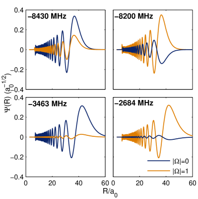
Figure 2: (Color online) Coriolis mixing between the $0_{u}^{+}$ and $1_{u}$ series. The upper two plots show the two-channel wavefunctions of the strongly mixed ⁸⁸Sr $J=1$ levels at $-8430$ MHz and $-8200$ MHz ($\theta=24^{\circ}$ and $\theta=114^{\circ}$, respectively). In the case of the $-8430$ MHz level, the $0_{u}^{+}$ component (dark blue lines) constitutes the majority of the two-channel wavefunction, while the $-8200$ MHz state is predominantly of the $1_{u}$ symmetry (orange lines). For comparison, in the lower part of the figure we show two relatively pure ($\theta=5^{\circ}$ and $\theta=95^{\circ}$) $0_{u}^{+}$ and $1_{u}$ states at $-3463$ MHz and $-2684$ MHz, respectively.

The Coriolis terms in the rotational Hamiltonian cause nonadiabatic mixing between the $0_{u}^{+}$ and $1_{u}$ components of the molecular wavefunction. This effect can be quantified by introducing a mixing angle $\theta$ defined by writing the total molecular wavefunction as:

$$\Psi(R)=\left(\cos\theta\,\tilde{\Psi}(0_{u}^{+};R),\sin\theta\,\tilde{\Psi}(1_{u};R)\right)^{T}\,.$$ (7)

Here we define the two reference functions $\tilde{\Psi}(0_{u}^{+};R)$ and $\tilde{\Psi}(1_{u};R)$, which are the two wavefunction components normalized separately via:

$$\tilde{\Psi}(0_{u}^{+};R)=\Psi(0_{u}^{+};R)\left(\int_{0}^{\infty}\Psi(0_{u}^{+};R)^{2}dR\right)^{-1/2}\,,$$ (8)

and

$$\tilde{\Psi}(1_{u};R) = \Psi(1_{u};R)\left(\int_{0}^{\infty}\Psi(1_{u};R)^{2}dR\right)^{-1/2}\times$$ (9)

$$\times\,{\rm sgn}\left(\int_{0}^{\infty}\Psi(0_{u}^{+};R)\Psi(1_{u};R)dR\right)\,.$$

The signum function above ensures that our phase convention is compatible with the one in Ref. McGuyer et al. (2013). It is straightforward to verify that with these definitions Eq. 7 yields a correctly normalized two-channel wavefunction. Finally, we note that the transformation $\theta\rightarrow\theta+180^{\circ}$ only changes the sign of the total wavefunction without altering its internal phase relationship. We therefore decide on having $0^{\circ}\leq\theta<180^{\circ}$, again in accordance with McGuyer et al. (2013). In this convention, a pure $0_{u}^{+}$ state has $\theta=0^{\circ}$ or $\theta\to 180^{\circ}$, while $\theta=90^{\circ}$ for a pure $1_{u}$ state.

Table 1 lists our Coriolis mixing angles $\theta$ for each of the considered energy levels. For completeness we also include mixing angles from Ref. McGuyer et al. (2013) which are in good agreement with ours. For two of the most deeply bound states in ⁸⁸Sr at $-8200$ MHz and $-8430$ MHz, McGuyer et al. give two different mixing angles as their theoretical model was not accurate enough to ascertain which of these two energy levels belong to the $0_{u}^{+}$ and $1_{u}$ series. In our model, however, the $-8200$ MHz line clearly belongs to the $1_{u}$ series, while the $-8430$ MHz has $0_{u}^{+}$ symmetry, confirming the original assignment of Zelevinsky et al. Zelevinsky et al. (2006).

Coriolis mixing is a significant factor in the bound state energies close to the ${}^{1}S_{0}$+${}^{3}P_{1}$ limit in strontium. Not surprisingly, the energy shift by this mixing is dependent on the mixing angle $\theta$. This is especially important for the very long range top bound states: for example, without Coriolis mixing the theoretical energy for the $-0.435$ MHz level in ⁸⁸Sr is $-0.160$ MHz. An even more extreme case is the top bound state in ⁸⁴Sr where the theoretical binding energy would be $-37$ kHz as opposed to the experimental value of $-0.32$ MHz. Moreover, Coriolis mixing is especially strong when two energy levels of $0_{u}^{+}$ and $1_{u}$ coincide, as is the case of the two energy levels in ⁸⁸Sr at $-8200$ MHz and $-8430$ MHz. The mixing angle $\theta=23^{\circ}$ for the $-8430$ MHz state, indicating particularly strong mixing, which again significantly influences the binding energy. In fact, without Coriolis mixing the respective theoretical energies are $-8234$ MHz and $-8394$ MHz, missing the experimental line positions by over $30$ MHz. These two states are shown in the upper part of Fig. 2. The remaining bound states have mixing angles of about $5^{\circ}$ for $0_{u}^{+}$ states and $\approx 95^{\circ}$ for $1_{u}$ symmetry and therefore are relatively pure, as shown for the $-3463$ MHz ($0_{u}^{+}$) and $-2684$ MHz ($1_{u}$) states in the lower part of Fig. 2.

Our theoretical model provides improved description of the nonadiabatic Coriolis mixing between the $0_{u}^{+}$ and $1_{u}$ states. Recently, McGuyer et al. McGuyer et al. (2013) gave experimentally determined linear Zeeman coefficients $g$ for the ⁸⁸Sr photoassociation lines, as well as their theoretical counterparts. The Zeeman coefficients

$$g=g_{at}\left(\frac{\sin^{2}\theta}{J(J+1)}+\frac{\sin 2\theta}{\sqrt{(J(J+1))}}P_{01}\right)$$ (10)

are highly sensitive both to the mixing angle $\theta$ and the overlap $P_{01}$ of the components $\tilde{\Psi}(0_{u}^{+};R)$ and $\tilde{\Psi}(1_{u};R)$:

$$P_{01}=\int_{0}^{\infty}\tilde{\Psi}(0_{u}^{+};R)\tilde{\Psi}(1_{u};R)dR\,.$$ (11)

The atomic $g$-factor $g_{at}=1.5$ for the ${}^{3}P_{1}$ electronic state.

A comparison of experimental and theoretical Zeeman $g$-factors from Ref. McGuyer et al. (2013) with our values calculated with Eq. 10 is given in Table 1. For relatively pure $0_{u}^{+}$ and $1_{u}$ energy levels our $g$-factor agree very well with the theoretical values in McGuyer et al. (2013). In the case, however, of the top bound state at $-0.4$ MHz our theoretical value is slightly closer to the one obtained in experiment. The most striking improvement is seen in the case of the two strongly Coriolis-mixed bound states at $-8200$ MHz and $-8430$ MHz. As noted previously, these two energy levels are notoriously difficult to describe theoretically and the model in McGuyer et al. (2013) fails to reproduce their experimental $g$-factors. Our model reduces the discrepancy between theory and experiment by a factor of three and while our model still does not fit to within experimental accuracy, it at least gives qualitative agreement. Since our mixing angles $\theta$ are in very good agreement, we attribute this improvement to the better description of the wavefunction overlap $P_{01}$, which was a necessary condition to correctly reproduce the impact of Coriolis mixing on the positions of these two energy levels. This further corroborates the validity of our long range van der Waals $C_{6}$, $C_{8}$ and resonant dipole $C_{3}$ coefficients. For completeness we also provided our Zeeman $g$-factors for the remaining PA lines, but no experimental data is currently available to compare.

VI Mass scaling perturbed

VI.1 Single channel mass scaling

A mass scaled model is an interaction model that is capable of reproducing the energy levels for all isotopomers of a given molecule by only changing the reduced mass. By its nature photoassociation spectroscopy is relatively insensitive to the details of the short range atomic interaction as it is predominantly used to measure the energies of bound states very close to the dissociation limit. This can be understood using the following simple reasoning. The energy splittings between the vibrational states (on the order of $1$ GHz) are very small compared to the depth of the potential curve (tens of THz). Consequently, bound states close to the dissociation limit share the same short range wavefunction (to within an amplitude constant) and only differ in the long range, where even such small energy differences will influence the location of the outer classical turning point and the long range wavefunction. Therefore, to a certain approximation, the vibrational splittings would be determined by the long range potential parameters, like $C_{6}$ and $C_{3}$ in our case. On the other hand, the starting point of the vibrational state ladder would be determined by the vibrational wavefunction’s phase $\phi$, as required by the Bohr-Sommerfeld quantization condition. Such a philosophy is the basis for the famous analytic expression for the $s$-wave scattering length of an $R^{-n}$ potential Gribakin and Flambaum (1993), as well as the semiclassical Leroy-Bernstein formulas LeRoy and Bernstein (1970).

As a consequence of the above reasoning, obtaining mass scaling in a single channel model would only require a potential curve with the correct long range part and the right behavior of the total phase $\phi$ as a function of the reduced mass. Such an approach has been discussed in detail in Borkowski et al. (2013). In the case of a single potential curve the total phase can be well approximated using the WKB integral:

$$\phi=\frac{1}{\hbar}\int_{R_{\rm in}}^{\infty}\sqrt{-2\mu V(R)}dR\,,$$ (12)

where $R_{\rm in}$ is the location of the inner classical turning point and $V$ is the interaction potential curve. It is evident that in this approach the total phase $\phi$ is proportional to $\sqrt{\mu}$ as long as the potential $V$ is mass-independent. In this paper we will assume that the potential $V$ is the same for all isotopes.

Following the Bohr-Sommerfeld quantization condition the quantity $n=\phi/\pi$ is closely related to the number of bound states supported by the interaction potential. On the other hand, the positions of the vibrational states only depend on the fractional part $\Delta n=n-\lfloor n\rfloor$. Slowly increasing $n$, by e.g. adjusting the depth of the potential curve, causes the bound state energies to shift deeper into the potential well. At some point this will cause a new bound state at the dissociation limit to emerge. Increasing $n$ by 1 (or, equivalently, the total phase $\phi$ by $\pi$) would amount to adding exactly one vibrational state to the potential, with the weakly bound states having similar vibrational energies as previously. If we assume that the interaction potential $V$ is mass-independent, then the quantity $n$ is proportional to $\sqrt{\mu}$. In this picture, mass scaling would amount to finding a potential curve which offers correct values of $\Delta n$ for each isotope. This can be achieved by simply fixing the correct number of bound states supported by the interaction potential. Such a strategy has been successfully implemented in a number of PA investigations Kitagawa et al. (2008); Borkowski et al. (2009, 2013).

In our case the long range interactions near the ${}^{1}S_{0}$$+$${}^{3}P_{1}$ asymptote are described by two Hund’s case (c) potentials, $0_{u}^{+}$ and $1_{u}$ coupled by Coriolis mixing. We note, however, that this mixing is relatively weak and only provides a small correction to most bound state energies. In fact, foregoing the Coriolis mixing altogether does not change the number of bound states supported by the two potentials together. Therefore, mass scaling of both series can to some extent be treated separately. We will first consider the mass scaling of energy levels of $0_{u}^{+}$ symmetry, for which most of the experimental data was collected. The final step will be the addition of the $1_{u}$ states to the model.

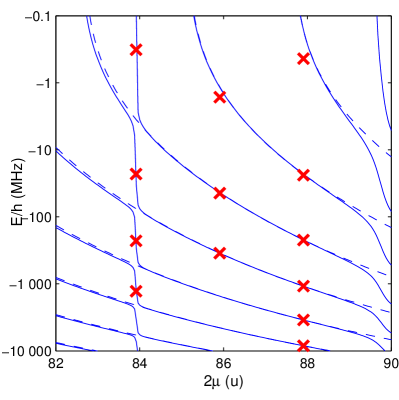
Figure 3: (Color online) Theoretical $0_{u}^{+}$ energy levels as a function of the reduced mass $\mu$. The blue dashed lines are calculated using the ${}^{3}\Pi_{u}$ potential curve alone which is only capable of mass scaling between two isotopes at a time — ⁸⁶Sr and ⁸⁸Sr in this case. The solid lines show the results for a model that also includes the short range crossing with a ${}^{1}S_{0}$+${}^{1}D_{2}$ ${}^{1}\Sigma_{u}^{+}$ potential, as shown in Fig. 4. The latter model is capable of reproducing the experimental bound state energies (marked as red crosses) for all isotopes. In this model, a short range ${}^{1}\Sigma_{u}^{+}$ perturbing state crosses the ${}^{1}S_{0}$$+$${}^{3}P_{1}$ dissociation limit at $2\mu\approx 84$ u causing a sudden departure from the usual mass scaling behavior.

Figure 3 shows the $0_{u}^{+}$ bound state energies as a function of the reduced mass. By changing the $\alpha(^{3}\Pi_{u})$ potential parameter we have found an appropriate $0_{u}^{+}$ potential depth (and consequently $\phi$) that correctly translated the wavefunction phase between the isotopes ⁸⁶Sr and ⁸⁸Sr. The results are shown in Fig. 3 as dashed lines. We have found that while our model fits the experimental bound state energies for ⁸⁶Sr and ⁸⁸Sr to within $1$ MHz (with the exception of the strongly Coriolis mixed $-8430$ MHz state), it is in shocking disagreement with the experimental data for ⁸⁴Sr.

This clear failure of mass scaling be easily explained a posteriori using the simple picture described earlier. The fractional part $\Delta n$ of the total WKB phase $\phi/\pi$ of the $0_{u}^{+}$ state (computed by applying Eq. 12 to $\mathcal{V}(^{3}\Pi_{u};R)$) for the best-fit models from Section III is $\Delta n=0.3928$, $0.6003$ and $0.3245$ for ⁸⁸Sr, ⁸⁶Sr, and ⁸⁴Sr, respectively. In the case of a single potential curve, $n$ scales linearly with $\sqrt{\mu}$. The model shown in Fig. 3 shows bound state energies calculated using a potential that has $n=69.3928$ and mass scales, correctly, to $n=68.6003$ for ⁸⁶Sr, which fits the observed line positions. Note that this model supports one bound state fewer for the latter isotope. For the ⁸⁴Sr isotope, however, mass scaling gives $n=67.7988$, but this fails to predict the observed line positions.

Similar mass scaling can be obtained for other numbers of bound states, but in all cases only for two isotopes at a time. For example, in the physically reasonable range of $50$ to $150$ supported bound states, mass scaling between ⁸⁸Sr and ⁸⁶Sr is obtained only for $69$ vibrational states, while for ⁸⁸Sr and ⁸⁴Sr the correct phases can be obtained for $89$ or $133$ states. Finally, for the ⁸⁶Sr-⁸⁴Sr pair a potential curve with $111$ bound states would support mass scaling. Clearly none of these numbers overlap. In fact, within this simple approximation no single potential curve supporting less than $300$ vibrational states could support mass scaling between all three isotopes. For comparison, an unmodified ${}^{3}\Pi_{u}$ curve from Skomorowski et al. (2012), as used in our model in Section III, supports a total of $72$ bound states for $J=1$ in ⁸⁸Sr.

VI.2 The avoided crossing

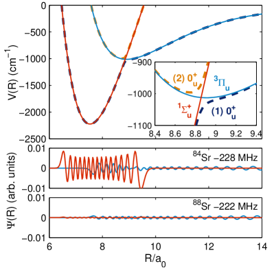
Figure 4: (Color online) Avoided crossing between the ¹S₀+³P₁ ${}^{3}\Pi_{u}$ and ¹S₀+${}^{1}D_{2}$ ${}^{1}\Sigma_{u}^{+}$ potential curves. The strong spin-orbit coupling between these two potential curves causes anomalies in the mass-scaling behavior of the photoassociation spectra near strontium intercombination line. In fact, a model that only includes the potential curve directly supporting the $0_{u}^{+}$ bound states close to the ¹S₀+³P₁ dissociation limit is incapable of properly describing mass scaling between the three bosonic isotopes in strontium.

Table 4: A comparison of experimental $0_{u}^{+}$ bound state energies with predictions of our mass-scaled model that includes the strong spin-orbit coupling between the ${}^{1}S_{0}$+${}^{3}P_{1}$ ${}^{3}\Pi_{u}$ curve which directly supports the $0_{u}^{+}$ series observed in PA experiments and the ${}^{1}S_{0}$+${}^{1}D_{2}$ ${}^{1}\Sigma_{u}^{+}$ curve. See text.

	88Sr		86Sr		84Sr
$\nu$	Exp.	Theory	Exp.	Theory	Exp.	Theory
-1	-0.435	-0.164	-1.633	-1.169	-0.320	-0.071
-2	-23.932	-23.133	-44.246	-43.467	-23.010	-23.208
-3	-222.161	-221.137	-348.742	-349.115	-228.380	-228.173
-4	-1084.093	-1083.353			-1288.290	-1062.636
-5	-3463.280	-3463.857
-6	-8429.650	-8410.027

It has recently been established, both experimentally Stein et al. (2010) and theoretically Skomorowski et al. (2012), that the ${}^{3}\Pi_{u}$ potential which supports the Hund’s case (c) $0_{u}^{+}$ potential correlating to the ¹S₀+³P₁ asymptote has a strong short range avoided crossing with a ${}^{1}\Sigma_{u}^{+}$ curve which corresponds to the much higher ¹S₀+¹D₂ asymptote. The resulting ¹S₀+³P₁ $0_{u}^{+}$ curve, as shown in Fig. 4, has several intriguing characteristics: its depth is defined almost solely by the depth of the ${}^{1}\Sigma_{u}^{+}$ potential and it enables nuclear motion at shorter distances than the ${}^{3}\Pi_{u}$ curve alone. Skomorowski et al.Skomorowski et al. (2012) have analyzed the composition of bound states in the $0_{u}^{+}$ state. The deepest bound states in the potential well are comprised primarily of the ${}^{1}\Sigma_{u}^{+}$ state, as expected given their energies are below the minimum of the ${}^{3}\Pi_{u}$ curve. As we move up the bound state ladder, the bound states become seemingly erratic mixtures of the ${}^{1}\Sigma_{u}^{+}$ and ${}^{3}\Pi_{u}$ states. Finally, the bound states closest to the dissociation limit (and so far investigated by photoassociation spectroscopy) are nearly pure ${}^{3}\Pi_{u}$ states, which explains why our long range model alone was enough to quantitatively describe most of the observed vibrational spacings.

To test the influence of the ${}^{1}\Sigma_{u}^{+}$ state on the ${}^{3}\Pi_{u}$ bound states and mass scaling we use a two channel model that includes both potentials:

$$V_{\rm int}=\left(\begin{array}[]{c c}\mathcal{V}(^{3}\Pi_{u};R)-C_{3,0}R^{-3}&\sigma\xi_{1}(R)\\ \sigma\xi_{1}(R)&\mathcal{V}(^{1}\Sigma_{u}^{+};R)+\Delta E\\ \end{array}\right)\,,$$ (13)

where, similar to Section III, $\mathcal{V}(^{1}\Sigma_{u}^{+};R)={V}({\rm A}^{1}\Sigma_{u}^{+};R)-{V}({\rm A}^{1}\Sigma_{u}^{+};\infty)$. This model obviously lacks the $1_{u}$ curve, and consequently, it does not include Coriolis mixing, limiting its accuracy to about $1$ MHz for bound states with small Coriolis mixing angles. The diagonal rotational terms are $B(R)(J(J+1)+2)$ and $B(R)J(J+1)$, respectively. The potential $V(^{3}\Pi_{u};R)$ has the same parameters as the one from Section III except for $\alpha(^{3}\Pi_{u})$, which we use to adjust the quantum defect. The ${V}({\rm A}^{1}\Sigma_{u}^{+};R)$ potential and spin-orbit coupling function $\xi_{1}(R)$ is the same as in Skomorowski et al. (2012). Again, we model the influence of the ¹S₀+¹P₁ ${}^{1}\Sigma_{u}^{+}$ curve by manually adding the resonant dipole $-C_{3,0}R^{-3}$ term. The two additional fitted parameters are $\sigma\approx 0.42$, which enabled the scaling of the spin-orbit mixing between the two potential curves, and $\Delta E\approx 6250~{}{\rm cm}^{-1}$ which controls the splitting between the ³P₁ and ¹D₂ atomic states. We use the latter parameter to fix the position of the perturbing short range ${}^{1}\Sigma_{u}^{+}$ bound state with respect to the ${}^{1}S_{0}$$+$${}^{3}P_{1}$ asymptote while retaining the original shape of the ${}^{1}\Sigma_{u}^{+}$ potential. As was the case previously (Section III), the theoretical energy levels are obtained by solving the coupled channel Schrödinger equation for the above potential matrix.

The solid lines in Figure 3 show the theoretical bound state energies calculated using the above two-channel model fitted to the experimental $0_{u}^{+}$ data for all isotopes using only three parameters: $\alpha(^{3}\Pi_{u})$, which as previously we used to adjust the short range wavefunction phase, the mixing parameter $\sigma$ that scales the ab initio Skomorowski et al. (2012) spin-orbit coupling function and the relative positions of the two potential curves $\Delta E$. The long range parameters, $C_{6}(^{3}\Pi_{u})$ and $C_{3,0}$ are shared with the previously discussed long range model from Section III. Apart from the ⁸⁴Sr $-1288$ MHz state discussed in detail in Section IV, and the strongly Coriolis mixed $-8430$ MHz state in ⁸⁸Sr, the energy levels are reproduced to within $1$ MHz. We note that the fitting itself was a very difficult process due to the seemingly erratic behavior of the model. This is caused by the mixing between the two diabatic potential curves ${}^{3}\Pi_{u}$ and ${}^{1}\Sigma_{u}^{+}$ being strongly dependent on the relative phases of the two components $\Psi({}^{3}\Pi_{u})$ and $\Psi({}^{1}\Sigma_{u}^{+})$ of the coupled channel wavefunction. This is shown in the bottom part of Fig. 4. In our fit the $-222$ MHz state of ⁸⁸Sr is a nearly pure ${}^{3}\Pi_{u}$ state, while the $-228$ MHz level in ⁸⁴Sr is strongly influenced by a short range ${}^{1}\Sigma_{u}^{+}$ component. Such a dramatic change of ${}^{1}\Sigma_{u}^{+}$ component amplitude is likely the result of a bound state of this symmetry coinciding with the ${}^{1}S_{0}$+${}^{3}P_{1}$ asymptote in ⁸⁴Sr.

The mass scaling behavior of this model (solid lines in Fig. 3) is similar to the single channel case (dashed lines) for the range of reduced masses of about $2\mu\approx 85\ldots 89$ u. However, when a short range ${}^{1}\Sigma_{u}^{+}$ bound state crosses the ${}^{1}S_{0}$$+$${}^{3}P_{1}$ dissociation limit, there is a sudden resonant departure as seen near $2\mu\approx 84$ u and $2\mu\approx 90$ u. Since the spin-orbit mixing is relatively strong, the width of this resonant structure is large and encompasses all bound states close to the dissociation limit together, resulting in an apparent change in the quantum defect. This explains why the vibrational spacings alone can be described by a single channel model even when the mixing is large. A comparison of the experimental $0_{u}^{+}$ energy levels with ones calculated from our mass scaled model is shown in Table 4. The accuracy of the model is about $1$ MHz for the majority of the experimental data and is mostly limited by the lack of Coriolis mixing.

VI.3 Impact on vibrational spacings

Table 5: A comparison of theoretical energy levels of $0_{u}^{+}$ symmetry calculated with (‘Perturbed’) and without (‘Adiabatic’) the spin-orbit mixing between the ${}^{1}\Sigma_{u}^{+}$ and ${}^{3}\Pi_{u}$ curves. The quantum defect has been adjusted in the adiabatic case so that the energy of the $\nu=-3$ bound state strictly matches the one predicted by the two-channel model. This ensures that any differences between the energy level predictions are caused by the way the models are constructed rather than quantum defects. In our model the ⁸⁴Sr bound states close to the dissociation limit are significantly perturbed by this mixing, which changes their vibrational splittings significantly. On the other hand the ⁸⁸Sr bound states remain relatively unchanged. This behavior can be used in the future to ascertain the location of the perturbing states. All values are given in MHz.

	84Sr		88Sr
$\nu$	Perturbed	Adiabatic	Perturbed	Adiabatic
-3	-228.4	-228.4	-222.2	-222.2
-4	-1063.3	-1147.6	-1087.0	-1086.8
-5	-3087.8	-3704.1	-3472.5	-3471.2
-6	-6983.4	-9024.2	-8426.4	-8419.9
-7	-13987.8	-18316.1	-17080.6	-17056.0

The available photoassociation data for $J=1$ states in ⁸⁸Sr and ⁸⁶Sr can be well described by a simple model that only includes the ${}^{3}\Pi_{u}$ ($0_{u}^{+}$) curve. Consequently, significant mixing between ${}^{3}\Pi_{u}$ and ${}^{1}\Sigma_{u}^{+}$ must occur for bound states deeper in the well. Perturbation theory dictates that the size of the ${}^{1}\Sigma_{u}^{+}$ contribution to an otherwise ${}^{3}\Pi_{u}$ bound state increases in the vicinity of a ${}^{1}\Sigma_{u}^{+}$ bound state.

A comparison of the bound state energies predicted by our adiabatic (single channel) and perturbed (two channel mass scaled) model is shown in Table 5 for isotopes ⁸⁴Sr and ⁸⁸Sr. For both isotopes we have adjusted the wavefunction phases so that the energies of the $\nu=-3$ bound state energies match. This way we ensure a fair comparison of vibrational splittings. In our model the perturbing short range ${}^{1}\Sigma_{u}^{+}$ bound state crosses the ${}^{1}S_{0}$$+$${}^{3}P_{1}$ dissociation limit when the reduced mass $2\mu\approx 84$ u. Consequently, there are significant differences in the bound state energies for $\nu=-5$ and deeper states. On the other hand, in the case of ⁸⁸Sr, the differences between the models are about an order of magnitude smaller. This shows that it will be possible to experimentally determine which of the isotopes has its ${}^{1}S_{0}$$+$${}^{3}P_{1}$ asymptote perturbed. In our model ⁸⁴Sr is the perturbed isotope, but given our limited knowledge of the strontium PA spectra, ⁸⁶Sr could be the perturbed isotope as well. The subtle discrepancies between the ⁸⁶Sr experimental data and our theoretical model from Section III might hint toward this hypothesis. This uncertainty can be resolved experimentally by simply measuring the bound state energies deeper in the potential well. One of the isotopes should clearly have its vibrational spacings incompatible with an interaction model that only includes the channels belonging to the ${}^{1}S_{0}$+${}^{3}P_{1}$ asymptote.

VI.4 Mass scaling of $1_{u}$ energy levels and the three channel model

The last step in the construction of our mass scaled model is the introduction of the $1_{u}$ molecular state. The interaction potential matrix, as expressed in the $\left\{0_{u}^{+}(^{3}\Pi_{u}),0_{u}^{+}(^{1}\Sigma_{u}^{+}),1_{u}(^{3}\Sigma_{u}^{+},^{3}\Pi_{u})\right\}$ Hund’s case (c) basis is now

$$V_{\rm int}=\left(\begin{array}[]{c c c}\begin{array}[]{c}\mathcal{V}(^{3}\Pi_{u};R)-\\ -C_{3,0}R^{-3}\end{array}&\sigma\xi_{1}(R)&0\\ \sigma\xi_{1}(R)&\begin{array}[]{c}\mathcal{V}(^{1}\Sigma_{u}^{+};R)+\\ +\Delta E\end{array}&0\\ 0&0&\begin{array}[]{c}\frac{1}{2}\big{(}\mathcal{V}(^{3}\Pi_{u};R)+\\ +\mathcal{V}(^{3}\Sigma^{+}_{u};R)\big{)}-\\ -{C_{3,1}}/{R^{3}}\end{array}\\ \end{array}\right)\,.$$ (14)

Similarly, the rotational Hamiltonian

$$V_{\rm rot}=\left(\begin{array}[]{c c c}J(J+1)+2&0&-\sqrt{4J(J+1)}\\ 0&J(J+1)&0\\ -\sqrt{4J(J+1)}&0&J(J+1)\\ \end{array}\right)\,$$ (15)

now contains the Coriolis mixing terms like the long range interaction model from Section III. The kinetic Hamiltonian $T$ is again diagonal and the energy levels are calculated by solving the set of coupled Schrödinger equations $H\Psi=E\Psi$ for $H=T+V_{\rm int}+V_{\rm rot}$ and the three channel wavefunction $\Psi$.

At this point reaching a mass scaled model for both $0_{u}^{+}$ and $1_{u}$ energy levels is relatively straightforward. Since the Coriolis mixing is a small correction to the $0_{u}^{+}$ energies we can hope that the mass scaling model utilizing the ${}^{3}\Pi_{u}$-${}^{1}\Sigma_{u}^{+}$ curve crossing will stand except for cosmetic corrections to its parameters.

Experimental $1_{u}$ energy level data is, to date, only available for the ⁸⁸Sr and ⁸⁶Sr isotopes. We can therefore apply the single channel mass scaling strategy as described in Section VI.1, that is, fix the right number of bound states supported by the $1_{u}$ state. To this end, we have modified the short range $\alpha(^{3}\Sigma_{u}^{+})$ parameter, which only affects the $1_{u}$ quantum defect. Finally, we have run a least-squares optimization for both quantum defect $\alpha$ parameters and the curve crossing parameters $\Delta E$ and $\sigma$ in order to obtain the final fit. All of the long range parameters ($C_{3,0}$, as well as $C_{6}$ and $C_{8}$ for both potential curves) remain the same.

A comparison of experimental energy levels for all strontium isotopes with those predicted by our final three channel model is shown in Table 6. Apart from the ⁸⁴Sr $-1288$ MHz state discussed at length in Section IV and not included in this table, the theoretical energy levels match their experimental counterparts to about 0.5 MHz on average. Mass scaling between states of $1_{u}$ symmetry is acceptable, although we note that theoretical position of the ⁸⁶Sr state at $-159$ MHz is shifted by about 3 MHz. We have attempted to improve the accuracy of this fit by changing the number of bound states supported by the $1_{u}$ curve, but this resulted in a similar shift in the other direction.

For each bound state we also list channel contributions $c_{i}$ calculated using $c_{i}=\int_{0}^{\infty}\left|\Psi_{i}(R)\right|^{2}dR$ and normalized via $c_{1}+c_{2}+c_{3}=1$. The channel contributions again show the nonadiabatic effects described throughout this paper. For instance, the Coriolis mixing between the ${}^{1}S_{0}$+${}^{3}P_{1}$ $0_{u}^{+}$ and $1_{u}$ states is clearly visible in the top $0_{u}^{+}$ bound states of ⁸⁴Sr and ⁸⁸Sr, where the $1_{u}$ contribution reaches about $10~{}\%$. Similarly the pair of $-8$ GHz states in ⁸⁸Sr is again very strongly mixed with mutual contributions as high as $14$ %. On the other hand, the short range mixing between the two $0_{u}^{+}$ states only significantly affects the ⁸⁴Sr isotope with contributions up to $3.9~{}\%$ for the $-228$ MHz state while for the remaining isotopes it is below $0.04$ % and as such is insignificant.

Table 6: Final $0_{u}^{+}$ and $1_{u}$ bound state energies as calculated from our three channel mass scaled model described in Sec. VI.4. Channel contributions are also given.

	Energy levels (MHz)		Channel contributions (%)
Isotope	Experiment	Theory	$0_{u}^{+}(^{3}\Pi_{u})$	$0_{u}^{+}(^{1}\Sigma_{u}^{+})$	$1_{u}(^{3}\Sigma_{u}^{+},^{3}\Pi_{u})$
88Sr	-0.435	-0.426	90.991	0.000	9.009
	-23.932	-23.856	98.881	0.000	1.118
	-222.161	-222.021	99.499	0.003	0.498
	-353.236	-352.934	0.462	0.000	99.538
	-1084.093	-1083.648	99.597	0.009	0.393
	-2683.722	-2683.117	0.730	0.000	99.270
	-3463.280	-3463.434	99.252	0.022	0.726
	-8200.163	-8199.777	14.194	0.006	85.800
	-8429.650	-8431.909	85.764	0.036	14.200
86Sr	-1.633	-1.535	94.991	0.000	5.009
	-44.246	-43.864	98.785	0.000	1.215
	-159.984	-163.296	1.628	0.000	98.372
	-348.742	-348.925	98.624	0.001	1.375
84Sr	-0.320	-0.341	89.470	0.025	10.505
	-23.010	-23.541	89.183	0.548	10.269
		-32.855	10.125	0.074	89.800
	-228.380	-228.259	95.130	3.912	0.957
		-1023.648	88.505	11.229	0.266
		-1472.635	0.206	0.135	99.660

VII Conclusion

In conclusion we have measured the energies of four vibrational bound states of the ⁸⁶Sr molecule in an excited triplet state using photoassociation spectroscopy of ultracold strontium atoms. The obtained data complements previously reported photoassociation data for the remaining two bosonic isotopes of strontium: ⁸⁴Sr and ⁸⁸Sr. We have provided an ab initio based theoretical model that correctly describes Coriolis mixing between $0_{u}^{+}$ and $1_{u}$ states. Only one of the previously reported energy levels, in ⁸⁴Sr, is in qualitative disagreement with our theory and we have suggested that it may either be supported by a different potential curve, or be strongly perturbed. We have used our theoretical model to provide Zeeman $g$-factors for all of the considered photoassociation lines.

We have also shown, however, that a theoretical model that only takes into account the two potential curves correlating to the ¹S₀+³P₁ asymptote will fail to correctly describe the positions of energy levels for all isotopes via simple mass scaling, even despite being correct for one isotope at a time. We attribute that to the short range avoided crossing between the ¹S₀+³P₁ ${}^{3}\Pi_{u}$ curve and a higher excited state ¹S₀+¹D₂ ${}^{1}\Sigma_{u}^{+}$ potential: a short range ${}^{1}\Sigma_{u}^{+}$ bound state would perturb the positions of the series of states observed in photoassociation spectroscopy near the intercombination line. We have produced a three channel model that take this mixing into account and is capable of reproducing the available $0_{u}^{+}$ and $1_{u}$ energy levels. Finally, we suggest that this theory can be tested by measuring more deeply bound vibrational states. For at least one isotope the vibrational spacings should significantly depart from those predicted by the long range model alone.

The results shown here will be important in the research concerning optical Feshbach resonances near the intercombination line in Sr. The four resonances reported in the paper can now be used to control the interactions between ⁸⁶Sr atoms in a similar manner as it was done in ⁸⁸Sr Blatt et al. (2011); Yan et al. (2013). The mixing between states could also influence the possible use of Sr as a means for measuring changes in the $m_{p}/m_{e}$ ratio DeMille et al. (2008); Kotochigova et al. (2009). The findings here also provide a template for the description of mass scaling perturbed by short range avoided crossings in other similar systems: a similar crossing between ${}^{3}\Pi_{u}$ and ${}^{1}\Sigma_{u}^{+}$ potentials has already been found in the calcium system Allard et al. (2005).

Appendix A Fitting Photoassociation Spectra

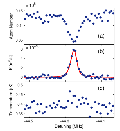
Figure 5: (Color online) Spectroscopy of the $0_{u}^{+}(\nu=-2)$ PA line of ⁸⁶Sr. (a) Atom number versus laser detuning from the one-photon ¹S${}_{0}-^{3}$P₁ atomic transition for interaction time $t=59.4$ ms. (b) The effective collision event rate constant derived from the atom loss using Eq. 19. (c) Temperature versus detuning shows little variation, supporting the assumption of constant sample temperature.

Table 7: Values of parameters of ⁸⁶Sr PA lines extracted from the experiment. Bound state energies are given for the $\nu=-1,-2,-3$ levels of $0_{u}^{+}$ symmetry and the $\nu=-1$ level of $1_{u}$ symmetry, where $\nu$ counts levels down from the dissociation limit. These levels all have angular momentum $J=1$. We also report the optical lengths $l_{\rm opt}$ for each of the measured $0_{u}^{+}$ PA lines. The term $\eta^{\rm upper}$ describes the additional molecular loss factor Theis et al. (2004); Blatt et al. (2011) and $\gamma^{\rm upper}_{\rm laser}$ is the upper limit on the PA laser line width.

$\nu$	86Sr	$\nu_{0}$ [MHz]	$l_{\textrm{opt}}/I$[$a_{\textrm{B}}$/(W/cm2)]	$\eta^{\textrm{upper}}$	$\gamma_{\textrm{laser}}^{\textrm{upper}}/2\pi$
	Series				[kHz]
-1	$0_{u}^{+}$	-1.633(10)	$(3.8\sim 6.5)\times 10^{4}$	1.7	10.5
-2	$0_{u}^{+}$	-44.246(10)	$(1.2\sim 1.8)\times 10^{4}$	1.5	7.5
-1	$1_{u}$	-159.984(50)	–	–	–
-3	$0_{u}^{+}$	-348.742(10)	$(5.7\sim 10.3)\times 10^{2}$	1.8	12.0

Experiments determine the number of atoms in the trap after exposure to the PA laser at frequency $f$ for interaction time $t$. Assuming constant sample temperature, and loss described by $\dot{n}=-2Kn^{2}$, the time evolution of the number of atoms is given by

$$N(t)=\frac{N_{0}}{1+2N_{0}KtV_{2}/V_{1}^{2}},$$ (16)

where $N_{0}$ is the number of atoms without applying PA beams, $K$ is the effective collision event rate constant, and $V_{q}$ ($q=1$ and 2) are the effective volumes defined by

$$V_{q}=\int d^{3}\!r\,e^{-qU(r)/k_{B}T},$$ (17)

with the trap potential $U(r)$, the Boltzmann constant $k_{B}$, and the sample temperature $T$. For a high ratio of trap depth to temperature, $\varepsilon_{t}/k_{B}T$, the effective volumes can be approximated by

$$V_{q}=\biggr{(}\frac{2\pi k_{B}T}{qm\overline{\omega}^{2}}\biggr{)}^{3/2},$$ (18)

where $m$ is the atomic mass, and $\overline{\omega}$ is the geometric mean of the angular oscillator frequencies of the trap. Equations 16 and 18 yield

$$K=\frac{4}{t}\biggl{(}\frac{1}{N(t)}-\frac{1}{N_{0}}\biggl{)}\biggl{(}\frac{\pi k_{B}T}{m\overline{\omega}^{2}}\biggl{)}^{3/2},$$ (19)

which allows direct determination of spectra of $K$ from the atom-loss spectra. Figure 5 is an example near the $0_{u}^{+}(\nu\,=\,-2)$ PA line of ⁸⁶Sr.

The spectra of collision event rate constant $K$ (Fig. 5 (b)) are fit using the formalism of Ciuryło et al. Ciuryło et al. (2004). This accounts for Doppler broadening and photon recoil, which is necessary when the atomic temperature $T$ is lower than the atomic recoil temperature $T_{R}=(h/\lambda)^{2}/(mk_{B})=460$ nK, for wavelength of the PA laser $\lambda=689$ nm. In our experiments, the sample temperature is $T\sim 400$ nK. In this regime, the collision event rate constant is given by Ciuryło et al. (2004)

$$K = \frac{k_{B}T}{hQ_{T}}\int_{-\infty}^{+\infty}dy\,e^{-y^{2}}\int_{0}^{\infty}dx\,x\,e^{-x^{2}}\mathcal{L}(f,y,x^{2}),$$ (20)

where $x$ and $y$ are dimensionless variables, and

$$\mathcal{L}(f,y,x^{2})={\eta\gamma_{\rm{mol}}{\gamma}_{s}/{(2\pi)^{2}}\over(f+y\Delta_{D}+x^{2}\Delta_{T}-E_{b}/h-E_{\rm{rec}}/h)^{2}+(\eta^{\prime}\gamma_{\rm{mol}}/4\pi)^{2}}.$$ (21)

with the thermal width $\Delta_{T}=k_{B}T/h$, the Doppler width $\Delta_{D}=\sqrt{k_{B}T/m}/\lambda$, the natural linewidth of the excited molecular level $\gamma_{\rm{mol}}=2\pi\times 15$ kHz, and the stimulated width $\gamma_{s}=2(\sqrt{2\mu x^{2}\Delta_{T}}/\hbar)\gamma_{\rm{mol}}\ell_{\rm{opt}}\ll\gamma_{\rm{mol}}$, where $\ell_{\rm{opt}}$ is the optical length. Here, $Q_{T}=\left({2\pi k_{B}T\mu/h^{2}}\right)^{3/2}$ is the partition function for reduced mass $\mu=m/2$, $h$ is Planck’s constant, $E_{b}$ is the PA line center including the molecular ac Stark shift due to PA beams, and $E_{\rm{rec}}=(h/\lambda)^{2}/(4m)$ is the photon recoil energy of an isolated atom. The parameter $\eta\geq 1$ accounts for the extra molecular losses observed in OFR experiments Theis et al. (2004); Blatt et al. (2011), and $\eta^{\prime}\gamma_{\rm{mol}}=\eta\gamma_{\rm{mol}}+\gamma_{\rm{laser}}$ with the line width of the PA laser $\gamma_{\rm{laser}}$. We can only determine $E_{\rm{b}}$, $\eta^{\prime}=\eta+\gamma_{\rm{laser}}/\gamma_{\rm{mol}}$, and $\eta\ell_{\rm{opt}}$, and cannot independently determine $\eta$, $\ell_{\rm{opt}}$, and $\gamma_{\rm{laser}}$. Truncation of the integral over collision kinetic energy has been neglected.

An example of the fitting result is shown in fig. 5 (b). The line center shifts linearly with the PA laser intensity, and we obtain spectra under a range of conditions and extrapolate to zero intensity to obtain the unshifted resonance position $\nu_{0}$ (Table 7). Fitting determines $\nu_{0}$ with a precision of 5 kHz. There is additional systematic error in determining the laser detuning with respect to atomic resonance of 5 kHz, and we quote a total uncertainty of 10 kHz (Table 7). The $\nu=-1$, $1_{u}$ binding energy is quoted with increased uncertainty because the data showed significant temperature variation, complicating the analysis. Further details of the experiment and the fitting procedure can be found in Yan (2013).

By linearly fitting the values of $\ell_{\rm{opt}}$ at different $I$, we extract $\ell_{\rm{opt}}/I$. The upper limit of $\eta$ ($\eta^{\rm{upper}}$) and the lower limit of $\ell_{\rm{opt}}$ can be determined by fixing $\gamma_{\rm{laser}}=0$, while the upper limit of $\gamma_{\rm{laser}}$ ($\gamma_{\rm{laser}}^{\rm{upper}}$,) and the upper limit of $\ell_{\rm{opt}}$ can be determined by fixing $\eta=1$. Values of these parameters from the fitting are summarized in Table 7.

References

- Jones et al. (2006) K. M. Jones, E. Tiesinga, P. D. Lett, and P. S. Julienne, Rev. Mod. Phys. 78, 483 (2006).
- Kahmann et al. (2014) M. Kahmann, E. Tiemann, O. Appel, U. Sterr, and F. Riehle, Phys. Rev. A 89, 023413 (2014).
- Zelevinsky et al. (2006) T. Zelevinsky, M. M. Boyd, A. D. Ludlow, T. Ido, J. Ye, R. Ciuryło, P. Naidon, and P. S. Julienne, Physical Review Letters 96, 203201 (2006).
- McGuyer et al. (2013) B. H. McGuyer, C. B. Osborn, M. McDonald, G. Reinaudi, W. Skomorowski, R. Moszynski, and T. Zelevinsky, Phys. Rev. Lett. 111, 243003 (2013).
- Stellmer et al. (2012) S. Stellmer, B. Pasquiou, R. Grimm, and F. Schreck, Physical Review Letters 109, 115302 (2012).
- Tojo et al. (2006) S. Tojo, M. Kitagawa, K. Enomoto, Y. Kato, Y. Takasu, M. Kumakura, and Y. Takahashi, Physical Review Letters 96, 153201 (2006).
- Borkowski et al. (2009) M. Borkowski, R. Ciuryło, P. S. Julienne, S. Tojo, K. Enomoto, and Y. Takahashi, Phys. Rev. A 80, 012715 (2009).
- Borkowski et al. (2011) M. Borkowski, R. Ciurylo, P. S. Julienne, R. Yamazaki, H. Hara, K. Enomoto, S. Taie, S. Sugawa, Y. Takasu, and Y. Takahashi, Physical Review A 84, 030702 (2011).
- Takasu et al. (2012) Y. Takasu, Y. Saito, Y. Takahashi, M. Borkowski, R. Ciuryło, and P. S. Julienne, Phys. Rev. Lett. 108, 173002 (2012).
- Ciuryło et al. (2004) R. Ciuryło, E. Tiesinga, S. Kotochigova, and P. S. Julienne, Phys. Rev. A 70, 062710 (2004).
- Skomorowski et al. (2012) W. Skomorowski, R. Moszynski, and C. P. Koch, Physical Review A 85, 043414 (2012).
- Ciuryło et al. (2005) R. Ciuryło, E. Tiesinga, and P. S. Julienne, Phys. Rev. A 71, 030701 (2005).
- Koch and Shapiro (2012) C. P. Koch and M. Shapiro, Chemical Reviews 112, 4928 (2012), http://pubs.acs.org/doi/pdf/10.1021/cr2003882 .
- Yan et al. (2013) M. Yan, B. J. DeSalvo, Y. Huang, P. Naidon, and T. C. Killian, Phys. Rev. Lett. 111, 150402 (2013).
- Kotochigova et al. (2009) S. Kotochigova, T. Zelevinsky, and J. Ye, Physical Review A 79, 012504 (2009).
- Martinez de Escobar et al. (2008) Y. N. Martinez de Escobar, P. G. Mickelson, P. Pellegrini, S. B. Nagel, A. Traverso, M. Yan, R. Côté, and T. C. Killian, Phys. Rev. A 78, 062708 (2008).
- Stein et al. (2008) A. Stein, H. Knöckel, and E. Tiemann, Phys. Rev. A 78, 042508 (2008).
- Stein et al. (2010) A. Stein, H. Knöckel, and E. Tiemann, European Physical Journal D 57, 171 (2010).
- Stein et al. (2011) A. Stein, H. Knoeckel, and E. Tiemann, European Physical Journal D 64, 227 (2011).
- Fedichev et al. (1996) P. O. Fedichev, Y. Kagan, G. V. Shlyapnikov, and J. T. M. Walraven, Phys. Rev. Lett. 77, 2913 (1996).
- Bohn and Julienne (1997) J. L. Bohn and P. S. Julienne, Phys. Rev. A 56, 1486 (1997).
- Chin et al. (2010) C. Chin, R. Grimm, P. Julienne, and E. Tiesinga, Reviews of Modern Physics 82, 1225 (2010).
- Lett et al. (1993) P. D. Lett, K. Helmerson, W. D. Phillips, L. P. Ratliff, S. L. Rolston, and M. E. Wagshul, Physical Review Letters 71, 2200 (1993).
- Fatemi et al. (2000) F. K. Fatemi, K. M. Jones, and P. D. Lett, Phys. Rev. Lett. 85, 4462 (2000).
- Theis et al. (2004) M. Theis, G. Thalhammer, K. Winkler, M. Hellwig, G. Ruff, R. Grimm, and J. H. Denschlag, Physical Review Letters 93, 123001 (2004).
- Thalhammer et al. (2005) G. Thalhammer, M. Theis, K. Winkler, R. Grimm, and J. H. Denschlag, Phys. Rev. A 71, 033403 (2005).
- Enomoto et al. (2008) K. Enomoto, K. Kasa, M. Kitagawa, and Y. Takahashi, Physical Review Letters 101, 203201 (2008), enomoto, K. Kasa, K. Kitagawa, M. Takahashi, Y.
- Blatt et al. (2011) S. Blatt, T. L. Nicholson, B. J. Bloom, J. R. Williams, J. W. Thomsen, P. S. Julienne, and J. Ye, Physical Review Letters 107, 073202 (2011).
- Yan et al. (2013) M. Yan, B. J. DeSalvo, B. Ramachandhran, H. Pu, and T. C. Killian, Physical Review Letters 110, 123201 (2013).
- Mickelson et al. (2005) P. G. Mickelson, Y. N. Martinez, A. D. Saenz, S. B. Nagel, Y. C. Chen, T. C. Killian, P. Pellegrini, and R. Côté, Phys. Rev. Lett. 95, 223002 (2005).
- Ido et al. (2000) T. Ido, Y. Isoya, and H. Katori, Phys. Rev. A 61, 061403 (2000).
- Ferrari et al. (2006) G. Ferrari, R. E. Drullinger, N. Poli, F. Sorrentino, and G. M. Tino, Phys. Rev. A 73, 023408 (2006).
- Stellmer et al. (2009) S. Stellmer, M. K. Tey, B. Huang, R. Grimm, and F. Schreck, Physical Review Letters 103, 200401 (2009).
- de Escobar et al. (2009) Y. N. M. de Escobar, P. G. Mickelson, M. Yan, B. J. Desalvo, S. B. Nagel, and T. C. Killian, Physical Review Letters 103, 200402 (2009).
- Stellmer et al. (2010) S. Stellmer, M. K. Tey, R. Grimm, and F. Schreck, Phys. Rev. A 82, 041602 (2010).
- Mickelson et al. (2010) P. G. Mickelson, Y. N. Martinez de Escobar, M. Yan, B. J. DeSalvo, and T. C. Killian, Phys. Rev. A 81, 051601 (2010).
- Stellmer et al. (2013a) S. Stellmer, B. Pasquiou, R. Grimm, and F. Schreck, Physical Review Letters 110, 263003 (2013a).
- DeSalvo et al. (2010) B. J. DeSalvo, M. Yan, P. G. Mickelson, Y. N. Martinez de Escobar, and T. C. Killian, Phys. Rev. Lett. 105, 030402 (2010).
- Stellmer et al. (2013b) S. Stellmer, R. Grimm, and F. Schreck, Physical Review A 87, 013611 (2013b).
- Reinaudi et al. (2012) G. Reinaudi, C. B. Osborn, M. McDonald, S. Kotochigova, and T. Zelevinsky, Physical Review Letters 109, 115303 (2012).
- (41) B. H. McGuyer, M. McDonald, G. Z. Iwata, M. G. Tarallo, W. Skomorowski, R. Moszyński, and T. Zelevinsky, arXiv:1407.4752 [physics.atom-ph] .
- Tomza et al. (2011) M. Tomza, F. Pawlowski, M. Jeziorska, C. P. Koch, and R. Moszynski, Physical Chemistry Chemical Physics 13, 18893 (2011).
- Pasquiou et al. (2013) B. Pasquiou, A. Bayerle, S. M. Tzanova, S. Stellmer, J. Szczepkowski, M. Parigger, R. Grimm, and F. Schreck, Physical Review A 88, 023601 (2013).
- Skomorowski et al. (2012) W. Skomorowski, F. Pawłowski, C. P. Koch, and R. Moszynski, J. Chem. Phys. 136, 194306 (2012).
- Nagel et al. (2003) S. B. Nagel, C. E. Simien, S. Laha, P. Gupta, V. S. Ashoka, and T. C. Killian, Phys. Rev. A 67, 011401 (2003).
- Yan et al. (2011) M. Yan, R. Chakraborty, A. Mazurenko, P. G. Mickelson, Y. N. M. de Escobar, B. J. Desalvo, and T. C. Killian, Phys. Rev. A 83, 032705 (2011).
- Mies et al. (1978) F. H. Mies, W. J. Stevens, and M. Krauss, Journal of Molecular Spectroscopy 72, 303 (1978).
- Tang and Toennies (1984) K. T. Tang and J. P. Toennies, The Journal of Chemical Physics 80, 3726 (1984).
- King and van Vleck (1939) G. W. King and J. H. van Vleck, Physical Review 55, 1165 (1939).
- Tiesinga et al. (1998) E. Tiesinga, C. J. Williams, and P. S. Julienne, Phys. Rev. A 57, 4257 (1998).
- Mitroy and Zhang (2010) J. Mitroy and J. Y. Zhang, Mol. Phys. 108, 1999 (2010).
- Porsev et al. (2014) S. G. Porsev, M. S. Safronova, and C. W. Clark, to be submitted to Phys. Rev. A (2014).
- Safronova et al. (2013) M. Safronova, S. Porsev, U. Safronova, M. Kozlov, and C. Clark, Phys. Rev. A 87, 012509 (2013).
- (54) S. Stellmer, Private Communication.
- Stellmer et al. (2014) S. Stellmer, F. Schreck, and T. Killian, in Annual Review of Cold Atoms and Molecules, Vol. 2, edited by K. W. Madison, Y. Wang, A. M. Rey, and K. Bongs (2014) Chap. 1.
- Julienne (1996) P. S. Julienne, Journal of Research of the National Institute of Standards and Technology 101, 487 (1996).
- Gribakin and Flambaum (1993) G. F. Gribakin and V. V. Flambaum, Phys. Rev. A 48, 546 (1993).
- LeRoy and Bernstein (1970) R. J. LeRoy and R. B. Bernstein, The Journal of Chemical Physics 52, 3869 (1970).
- Borkowski et al. (2013) M. Borkowski, P. S. Żuchowski, R. Ciuryło, P. S. Julienne, D. Kędziera, L. Mentel, P. Tecmer, F. Münchow, C. Bruni, and A. Görlitz, Phys. Rev. A 88, 052708 (2013).
- Kitagawa et al. (2008) M. Kitagawa, K. Enomoto, K. Kasa, Y. Takahashi, R. Ciuryło, P. Naidon, and P. S. Julienne, Phys. Rev. A 77, 012719 (2008).
- DeMille et al. (2008) D. DeMille, S. Sainis, J. Sage, T. Bergeman, S. Kotochigova, and E. Tiesinga, Physical Review Letters 100, 043202 (2008).
- Allard et al. (2005) O. Allard, S. Falke, A. Pashov, O. Dulieu, H. Knöckel, and E. Tiemann, The European Physical Journal D - Atomic, Molecular, Optical and Plasma Physics 35, 483 (2005).
- Yan (2013) M. Yan, Optical Feshbach Resonances and Coherent Photoassociation in a Strontium BEC, Ph.D. thesis, Rice University (2013).