Distributed Stochastic Optimization of the Regularized Risk

Abstract

Many machine learning algorithms minimize a regularized risk, and stochastic optimization is widely used for this task. When working with massive data, it is desirable to perform stochastic optimization in parallel. Unfortunately, many existing stochastic optimization algorithms cannot be parallelized efficiently. In this paper we show that one can rewrite the regularized risk minimization problem as an equivalent saddle-point problem, and propose an efficient distributed stochastic optimization (DSO) algorithm. We prove the algorithm’s rate of convergence; remarkably, our analysis shows that the algorithm scales almost linearly with the number of processors. We also verify with empirical evaluations that the proposed algorithm is competitive with other parallel, general purpose stochastic and batch optimization algorithms for regularized risk minimization.

1 Introduction

Regularized risk minimization is a well-known paradigm in machine learning:

$$\min_{\mathbf{w}}P\left(\mathbf{w}\right):=\lambda\sum_{j}\phi_{j}\left(w_{j}\right)+\frac{1}{m}\sum_{i=1}^{m}\ell\left(\left\langle\mathbf{w},\mathbf{x}_{i}\right\rangle,y_{i}\right).$$ (1)

Here, we are given $m$ training data points $\mathbf{x}_{i}\in\mathbb{R}^{d}$ and their corresponding labels $y_{i}$, while $\mathbf{w}\in\mathbb{R}^{d}$ is the parameter of the model. Furthermore, $w_{j}$ denotes the $j$-th component of $\mathbf{w}$, while $\phi_{j}\left(\cdot\right)$ is a convex function which penalizes complex models. $\ell\left(\cdot,\cdot\right)$ is a loss function, which is convex in $\mathbf{w}$. Moreover, $\left\langle\cdot,\cdot\right\rangle$ denotes the Euclidean inner product, and $\lambda>0$ is a scalar which trades-off between the average loss and the regularizer. For brevity, we will use $\ell_{i}\left(\left\langle\mathbf{w},\mathbf{x}_{i}\right\rangle\right)$ to denote $\ell\left(\left\langle\mathbf{w},\mathbf{x}_{i}\right\rangle,y_{i}\right)$.

Many well-known models can be derived by specializing (1). For instance, if $y_{i}\in\left\{\pm 1\right\}$, then setting $\phi_{j}(w_{j})=\frac{1}{2}w_{j}^{2}$ and $\ell_{i}\left(\left\langle\mathbf{w},\mathbf{x}_{i}\right\rangle\right)=\max\left(0,1-y_{i}\left\langle\mathbf{w},\mathbf{x}_{i}\right\rangle\right)$ recovers binary linear support vector machines (SVMs) [23]. On the other hand, using the same regularizer but changing the loss function to $\ell_{i}\left(\left\langle\mathbf{w},\mathbf{x}_{i}\right\rangle\right)=\log\left(1+\exp\left(-y_{i}\left\langle\mathbf{w},\mathbf{x}_{i}\right\rangle\right)\right)$ yields regularized logistic regression [11]. Similarly, setting $\phi_{j}\left(w_{j}\right)=\left|w_{j}\right|$ leads to sparse learning such as LASSO [11] with $\ell_{i}\left(\left\langle\mathbf{w},\mathbf{x}_{i}\right\rangle\right)=\frac{1}{2}\left(y_{i}-\left\langle\mathbf{w},\mathbf{x}_{i}\right\rangle\right)^{2}$.

A number of specialized as well as general purpose algorithms have been proposed for minimizing the regularized risk. For instance, if both the loss and the regularizer are smooth, as is the case with logistic regression, then quasi-Newton algorithms such as L-BFGS [17] have been found to be very successful. On the other hand, for smooth regularizers but non-smooth loss functions, Teo et al. [28] proposed a bundle method for regularized risk minimization (BMRM). Another popular first-order solver is Alternating Direction Method of Multipliers (ADMM) [5]. These optimizers belong to the broad class of batch minimization algorithms; that is, in order to perform a parameter update, at every iteration they compute the regularized risk $P(\mathbf{w})$ as well as its gradient

$$\nabla P\left(\mathbf{w}\right)=\lambda\sum_{j=1}^{d}\nabla\phi_{j}\left(w_{j}\right)\cdot\mathbf{e}_{j}+\frac{1}{m}\sum_{i=1}^{m}\nabla\ell_{i}\left(\left\langle\mathbf{w},\mathbf{x}_{i}\right\rangle\right)\cdot\mathbf{x}_{i},$$ (2)

where $\mathbf{e}_{j}$ denotes the $j$-th standard basis vector. Both $P\left(\mathbf{w}\right)$ as well as the gradient $\nabla P\left(\mathbf{w}\right)$ take $O(md)$ time to compute, which is computationally expensive when $m$, the number of data points, is large. Batch algorithms can be efficiently parallelized, however, by exploiting the fact that the empirical risk $\frac{1}{m}\sum_{i=1}^{m}\ell_{i}\left(\left\langle\mathbf{w},\mathbf{x}_{i}\right\rangle\right)$ as well as its gradient $\frac{1}{m}\sum_{i=1}^{m}\nabla\ell_{i}\left(\left\langle\mathbf{w},\mathbf{x}_{i}\right\rangle\right)\cdot\mathbf{x}_{i}$ decompose over the data points, and therefore one can compute $P\left(\mathbf{w}\right)$ and $\nabla P\left(\mathbf{w}\right)$ in a distributed fashion [7].

Batch algorithms, unfortunately, are known to be unfavorable for large scale machine learning both empirically and theoretically [3]. It is now widely accepted that stochastic algorithms which process one data point at a time are more effective for regularized risk minimization. In a nutshell, the idea here is that (2) can be stochastically approximated by

$$\mathbf{g}_{i}=\lambda\sum_{j=1}^{d}\nabla\phi_{j}\left(w_{j}\right)\cdot\mathbf{e}_{j}+\nabla\ell_{i}\left(\left\langle\mathbf{w},\mathbf{x}_{i}\right\rangle\right)\cdot\mathbf{x}_{i},$$ (3)

when $i$ is chosen uniformly random in $\left\{1,\ldots,m\right\}$. Note that $\mathbf{g}_{i}$ is an unbiased estimator of the true gradient $\nabla P\left(\mathbf{w}\right)$; that is, $\mathbb{E}_{i\in\left\{1,\ldots,m\right\}}\left[\mathbf{g}_{i}\right]=\nabla P\left(\mathbf{w}\right)$. Now we can replace the true gradient by this stochastic gradient to approximate a gradient descent update as

$$\mathbf{w}\leftarrow\mathbf{w}-\eta\cdot\mathbf{g}_{i},$$ (4)

where $\eta$ is a step size parameter. Computing $\mathbf{g}_{i}$ only takes $O(d)$ effort, which is independent of $m$, the number of data points. Bottou and Bousquet [3] show that stochastic optimization is asymptotically faster than gradient descent and other second-order batch methods such as L-BFGS for regularized risk minimization.

However, a drawback of update (4) is that it is not easy to parallelize anymore. Usually, the computation of $\mathbf{g}_{i}$ in (3) is a very lightweight operation for which parallel speed-up can rarely be expected. On the other hand, one cannot execute multiple updates of (4) simultaneously, since computing $\mathbf{g}_{i}$ requires reading the latest value of $\mathbf{w}$, while updating (4) requires writing to the components of $\mathbf{w}$. The problem is even more severe in distributed memory systems, where the cost of communication between processors is significant.

Existing parallel stochastic optimization algorithms try to work around these difficulties in a somewhat ad-hoc manner (see Section 4). In this paper, we take a fundamentally different approach and propose a reformulation of the regularized risk (1), for which one can naturally derive a parallel stochastic optimization algorithm. Our technical contributions are:

• We reformulate regularized risk minimization as an equivalent saddle-point problem, and show that it can be solved via a new distributed stochastic optimization (DSO) algorithm.

• We prove $O\left(1/\sqrt{T}\right)$ rates of convergence for DSO, and show that it scales almost linearly with the number of processors.

• We verify with empirical evaluations that when used for training linear support vector machines (SVMs) or binary logistic regression models, DSO is comparable to general-purpose stochastic (e.g., Zinkevich et al. [34]) or batch (e.g., Teo et al. [28]) optimizers.

2 Reformulating Regularized Risk Minimization

We begin by reformulating the regularized risk minimization problem as an equivalent saddle-point problem. Towards this end, we first rewrite (1) by introducing an auxiliary variable $u_{i}$ for each $\mathbf{x}_{i}$:

$$\min_{\mathbf{w},\mathbf{u}}\;\;\lambda\sum_{j=1}^{d}\phi_{j}\left(w_{j}\right)+\frac{1}{m}\sum_{i=1}^{m}\ell_{i}\left(u_{i}\right)\mathrm{s.t.}\;\;u_{i}=\left\langle\mathbf{w},\mathbf{x}_{i}\right\rangle\quad\forall\,\,i=1,\ldots,m.$$ (5)

By introducing Lagrange multipliers $\alpha_{i}$ to eliminate the constraints, we obtain

$$\min_{\mathbf{w},\mathbf{u}}\max_{\bm{\alpha}}\lambda\sum_{j=1}^{d}\phi_{j}\left(w_{j}\right)+\frac{1}{m}\sum_{i=1}^{m}\ell_{i}\left(u_{i}\right)+\frac{1}{m}\sum_{i=1}^{m}\alpha_{i}(u_{i}-\left\langle\mathbf{w},\mathbf{x}_{i}\right\rangle).$$

Here $\mathbf{u}$ denotes a vector whose components are $u_{i}$. Likewise, $\bm{\alpha}$ is a vector whose components are $\alpha_{i}$. Since the objective function (5) is convex and the constraints are linear, strong duality applies [4]. Therefore, we can switch the maximization over $\bm{\alpha}$ and the minimization over $\mathbf{w},\mathbf{u}$. Note that $\min_{u_{i}}\alpha_{i}u_{i}+\ell_{i}(u_{i})$ can be written $-\ell_{i}^{\star}(-\alpha_{i})$, where $\ell_{i}^{\star}(\cdot)$ is the Fenchel-Legendre conjugate of $\ell_{i}(\cdot)$ [4]. The above transformations yield to our formulation:

$$\max_{\bm{\alpha}}\min_{\mathbf{w}}f\left(\mathbf{w},\bm{\alpha}\right):=\lambda\sum_{j=1}^{d}\phi_{j}\left(w_{j}\right)-\frac{1}{m}\sum_{i=1}^{m}\alpha_{i}\left\langle\mathbf{w},\mathbf{x}_{i}\right\rangle-\frac{1}{m}\sum_{i=1}^{m}\ell^{\star}_{i}\left(-\alpha_{i}\right).$$

If we analytically minimize $f(\mathbf{w},\bm{\alpha})$ in terms of $\mathbf{w}$ to eliminate it, then we obtain so-called dual objective which is only a function of $\bm{\alpha}$. Moreover, any $\mathbf{w}^{*}$ which is a solution of the primal problem (1), and any $\bm{\alpha}^{*}$ which is a solution of the dual problem, is a saddle point of $f\left(\mathbf{w},\bm{\alpha}\right)$ [4]. In other words, minimizing the primal, maximizing the dual, and finding a saddle point of $f\left(\mathbf{w},\bm{\alpha}\right)$ are all equivalent problems.

2.1 Stochastic Optimization

Let $x_{ij}$ denote the $j$-th coordinate of $\mathbf{x}_{i}$, and $\Omega_{i}:=\left\{j:x_{ij}\neq 0\right\}$ denote the non-zero coordinates of $\mathbf{x}_{i}$. Similarly, let $\bar{\Omega}_{j}:=\left\{i:x_{ij}\neq 0\right\}$ denote the set of data points where the $j$-th coordinate is non-zero and $\Omega:=\left\{\left(i,j\right):x_{ij}\neq 0\right\}$ denotes the set of all non-zero coordinates in the training dataset $\mathbf{x}_{1},\ldots,\mathbf{x}_{m}$. Then, $f(\mathbf{w},\bm{\alpha})$ can be rewritten as

$$f\left(\mathbf{w},\bm{\alpha}\right)=\sum_{\left(i,j\right)\in\Omega}\frac{\lambda\phi_{j}\left(w_{j}\right)}{\left|\bar{\Omega}_{j}\right|}-\frac{\ell^{\star}_{i}(-\alpha_{i})}{m\left|\Omega_{i}\right|}-\frac{\alpha_{i}w_{j}x_{ij}}{m}=\sum_{\left(i,j\right)\in\Omega}f_{i,j}\left(w_{j},\alpha_{i}\right),$$ (6)

where $|\cdot|$ denotes the cardinality of a set. Remarkably, each component $f_{i,j}$ in the above summation depends only on one component $w_{j}$ of $\mathbf{w}$ and one component $\alpha_{i}$ of $\bm{\alpha}$. This allows us to derive an optimization algorithm which is stochastic in terms of both $i$ and $j$. Let us define

$$\mathbf{g}_{i,j}:=\Bigg{(}\left|\Omega\right|\left(\frac{\lambda\nabla\phi_{j}\left(w_{j}\right)}{\left|\bar{\Omega}_{j}\right|}-\frac{\alpha_{i}x_{ij}}{m}\right)\mathbf{e}_{j},\left|\Omega\right|\left(\frac{\nabla\ell^{\star}_{i}(-\alpha_{i})}{m\left|\Omega_{i}\right|}-\frac{w_{j}x_{ij}}{m}\right)\mathbf{e}_{i}\Bigg{)}.$$ (7)

Under the uniform distribution over $\left(i,j\right)\in\Omega$, one can easily see that $\mathbf{g}_{i,j}$ is an unbiased estimate of the gradient of $f\left(\mathbf{w},\bm{\alpha}\right)$, that is, $\mathbb{E}_{\left\{\left(i,j\right)\in\Omega\right\}}\left[\mathbf{g}_{i,j}\right]=\left(\nabla_{\mathbf{w}}f\left(\mathbf{w},\bm{\alpha}\right),-\nabla_{\bm{\alpha}}{-f}\left(\mathbf{w},\bm{\alpha}\right)\right)$. Since we are interested in finding a saddle point of $f\left(\mathbf{w},\bm{\alpha}\right)$, our stochastic optimization algorithm uses the stochastic gradient $\mathbf{g}_{i,j}$ to take a descent step in $\mathbf{w}$ and an ascent step in $\bm{\alpha}$ [19]:

$$w_{j}\leftarrow w_{j}-\eta\cdot\left(\frac{\lambda\nabla\phi_{j}\left(w_{j}\right)}{\left|\bar{\Omega}_{j}\right|}-\frac{\alpha_{i}x_{ij}}{m}\right),\text{ and }\alpha_{i}\leftarrow\alpha_{i}+\eta\cdot\left(\frac{\nabla\ell^{\star}_{i}(-\alpha_{i})}{m\left|\Omega_{i}\right|}-\frac{w_{j}x_{ij}}{m}\right).$$ (8)

Surprisingly, the time complexity of update (8) is independent of the size of data; it is $O(1)$. Compare this with the $O(md)$ complexity of batch update and $O(d)$ complexity of regular stochastic gradient descent.

Note that in the above discussion, we implicitly assumed that $\phi_{j}\left(\cdot\right)$ and $\ell_{i}^{\star}\left(\cdot\right)$ are differentiable. If that is not the case, then their derivatives can be replaced by sub-gradients [4]. Therefore this approach can deal with wide range of regularized risk minimization problem.

3 Parallelization

The minimax formulation (6) not only admits an efficient stochastic optimization algorithm, but also allows us to derive a distributed stochastic optimization (DSO) algorithm. The key observation underlying DSO is the following: Given $\left(i,j\right)$ and $\left(i^{\prime},j^{\prime}\right)$ both in $\Omega$, if $i\neq i^{\prime}$ and $j\neq j^{\prime}$ then one can simultaneously perform update (8) on $(w_{j},\alpha_{i})$ and $(w_{j^{\prime}},\alpha_{i^{\prime}})$. In other words, the updates to $w_{j}$ and $\alpha_{i}$ are independent of the updates to $w_{j^{\prime}}$ and $\alpha_{i^{\prime}}$, as long as $i\neq i^{\prime}$ and $j\neq j^{\prime}$.

Before we formally describe DSO we would like to present some intuition using Figure 1. Here we assume that we have 4 processors. The data matrix $X$ is an $m\times d$ matrix formed by stacking $\mathbf{x}_{i}^{\top}$ for $i=1,\ldots,m$, while $\mathbf{w}$ and $\bm{\alpha}$ denote the parameters to be optimized. The non-zero entries of $X$ are marked by an $\mathrm{x}$ in the figure. Initially, both parameters as well as rows of the data matrix are partitioned across processors as depicted in Figure 1 (left); colors in the figure denote ownership e.g., the first processor owns a fraction of the data matrix and a fraction of the parameters $\bm{\alpha}$ and $\mathbf{w}$ (denoted as $\mathbf{w}^{\left(1\right)}$ and $\bm{\alpha}^{\left(1\right)}$) shaded with red. Each processor samples a non-zero entry $x_{ij}$ of $X$ within the dark shaded rectangular region (active area) depicted in the figure, and updates the corresponding $w_{j}$ and $\alpha_{i}$. After performing updates, the processors stop and exchange coordinates of $\mathbf{w}$. This defines an inner iteration. After each inner iteration, ownership of the $\mathbf{w}$ variables and hence the active area change, as shown in Figure 1 (right). If there are $p$ processors, then $p$ inner iterations define an epoch. Each coordinate of $\mathbf{w}$ is updated by each processor at least once in an epoch. The algorithm iterates over epochs until convergence.

Four points are worth noting. First, since the active area of each processor does not share either row or column coordinates with the active area of other processors, as per our key observation above, the updates can be carried out by each processor in parallel without any need for intermediate communication with other processors. Second, we partition and distribute the data only once. The coordinates of $\bm{\alpha}$ are partitioned at the beginning and are not exchanged by the processors; only coordinates of $\mathbf{w}$ are exchanged. This means that the cost of communication is independent of $m$, the number of data points. Third, our algorithm can work in both shared memory, distributed memory, and hybrid (multiple threads on multiple machines) architectures. Fourth, the $\mathbf{w}$ parameter is distributed across multiple machines and there is no redundant storage, which makes the algorithm scale linearly in terms of space complexity. Compare this with the fact that most parallel optimization algorithms require each local machine to hold a copy of $\mathbf{w}$.

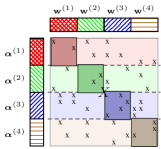
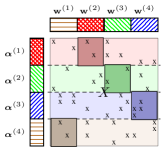
Figure 1: Illustration of DSO with 4 processors. The rows of the data matrix $X$ as well as the parameters $\mathbf{w}$ and $\bm{\alpha}$ are partitioned as shown. Colors denote ownerships. The active area of each processor is in dark colors. Left: the initial state. Right: the state after one bulk synchronization.

To formally describe DSO, suppose $p$ processors are available, and let $I_{1},\ldots,I_{p}$ denote a fixed partition of the set $\left\{1,\ldots,m\right\}$ and $J_{1},\ldots,J_{p}$ denote a fixed partition of the set $\left\{1,\ldots,d\right\}$ such that $\left|I_{q}\right|\approx\left|I_{q^{\prime}}\right|$ and $\left|J_{r}\right|\approx\left|J_{r^{\prime}}\right|$ for any $1\leq q,q^{\prime},r,r^{\prime}\leq p$. We partition the data $\left\{\mathbf{x}_{1},\ldots,\mathbf{x}_{m}\right\}$ and the labels $\left\{y_{1},\ldots,y_{m}\right\}$ into $p$ disjoint subsets according to $I_{1},\ldots,I_{p}$ and distribute them to $p$ processors. The parameters $\left\{\alpha_{1},\ldots,\alpha_{m}\right\}$ are partitioned into $p$ disjoint subsets $\bm{\alpha}^{(1)},\ldots,\bm{\alpha}^{(p)}$ according to $I_{1},\ldots,I_{p}$ while $\left\{w_{1},\ldots,w_{d}\right\}$ are partitioned into $p$ disjoint subsets $\mathbf{w}^{(1)},\ldots,\mathbf{w}^{(p)}$ according to $J_{1},\ldots,J_{p}$ and distributed to $p$ processors, respectively. The partitioning of $\left\{1,\ldots,m\right\}$ and $\left\{1,\ldots,d\right\}$ induces a $p\times p$ partition of $\Omega$:

$$\Omega^{(q,r)}:=\left\{(i,j)\in\Omega\;:\;i\in I_{q},j\in J_{r}\right\},\;\;q,r\in\left\{1,\ldots,p\right\}.$$

The execution of DSO proceeds in epochs, and each epoch consists of $p$ inner iterations; at the beginning of the $r$-th inner iteration ($r\geq 1$), processor $q$ owns $\mathbf{w}^{\left(\sigma_{r}\left(q\right)\right)}$ where $\sigma_{r}\left(q\right)=\left\{\left(q+r-2\right)\text{ mod }p\right\}+1$, and executes stochastic updates (8) on coordinates in $\Omega^{\left(q,\sigma_{r}\left(q\right)\right)}$. Since these updates only involve variables in $\bm{\alpha}^{\left(q\right)}$ and $\mathbf{w}^{\left(\sigma\left(q\right)\right)}$, no communication between processors is required to execute them. After every processor has finished its updates, $\mathbf{w}^{\left(\sigma_{r}\left(q\right)\right)}$ is sent to machine $\sigma_{r+1}^{-1}\left(\sigma_{r}\left(q\right)\right)$ and the algorithm moves on to the $(r+1)$-st inner iteration. Detailed pseudo-code for the DSO algorithm can be found in Algorithm 1.

1:  Each processor $q\in\left\{1,2,\ldots,p\right\}$ initializes $\mathbf{w}^{(q)}$, $\bm{\alpha}^{(q)}$

2:  $t\leftarrow 1$

3:  repeat

4:     $\eta_{t}\leftarrow\eta_{0}/\sqrt{t}$

5:     for all $r\in\left\{1,2,\ldots,p\right\}$ do

6:        for all processors $q\in\left\{1,2,\ldots,p\right\}$ in parallel do

7:           for $(i,j)\in\Omega^{(q,\sigma_{r}(q))}$ do

8:              $w_{j}\leftarrow w_{j}-\eta_{t}\cdot\left(\frac{\lambda\nabla\phi_{j}\left(w_{j}\right)}{\left|\bar{\Omega}_{j}\right|}-\frac{\alpha_{i}x_{ij}}{m}\right)$ and $\alpha_{i}\leftarrow\alpha_{i}+\eta_{t}\cdot\left(\frac{\nabla\ell^{\star}_{i}(-\alpha_{i})}{m\left|\Omega_{i}\right|}-\frac{w_{j}x_{ij}}{m}\right)$

9:           end for

10:           send $\mathbf{w}^{\left(\sigma_{r}(q)\right)}$ to machine $\sigma_{r+1}^{-1}(\sigma_{r}(q))$ and receive $\mathbf{w}^{\left(\sigma_{r+1}(q)\right)}$

11:        end for

12:     end for

13:     $t\leftarrow t+1$

14:  until convergence

Algorithm 1 Distributed stochastic optimization (DSO) for finding saddle point of (6)

3.1 Convergence Analysis

It is known that the stochastic procedure in section 2.1 is guaranteed to converge to the saddle point of $f(\mathbf{w},\bm{\alpha})$ [19]. The main technical difficulty in proving convergence in our case is because DSO does not sample $\left(i,j\right)$ coordinates uniformly at random due to its distributed nature. Therefore, first we prove that DSO is serializable in a certain sense, that is, there exists an ordering of the updates such that replaying them on a single machine would recover the same solution produced by DSO. We then analyze this serial algorithm to establish convergence. We believe that this proof technique is of independent interest, and differs significantly from convergence analysis for other parallel stochastic algorithms which typically assume correlation between data points [e.g. 16, 6].

Theorem 1.

Let $\left(\mathbf{w}^{t},\bm{\alpha}^{t}\right)$ and $\left(\tilde{\mathbf{w}}^{t},\tilde{\bm{\alpha}}^{t}\right):=\left(\frac{1}{t}\sum_{s=1}^{t}\mathbf{w}^{s},\frac{1}{t}\sum_{s=1}^{t}\bm{\alpha}^{s}\right)$ denote the parameter values, and the averaged parameter values respectively after the $t$-th epoch of Algorithm 1. Moreover, assume that $\left\|\mathbf{w}\right\|,\left\|\bm{\alpha}\right\|,\left|\nabla\phi_{j}(w_{j})\right|,\left|\nabla\ell_{i}^{\star}\left(-\alpha_{i}\right)\right|,$ and $\lambda$ are upper bounded by a constant $c>1$. Then, there exists a constant $C$, which is dependent only on $c$, such that after $T$ epochs the duality gap is

$$\varepsilon\left(\tilde{\mathbf{w}}^{T},\tilde{\bm{\alpha}}^{T}\right):=\max_{\bm{\alpha}^{\prime}}f\left(\tilde{\mathbf{w}}^{T},\bm{\alpha}^{\prime}\right)-\min_{\mathbf{w}^{\prime}}f\left(\mathbf{w}^{\prime},\tilde{\bm{\alpha}}^{T}\right)\leq C\frac{\sqrt{d}}{\sqrt{T}}.$$ (9)

On the other hand, if $\phi_{j}(s)=\frac{1}{2}s^{2}$, $\sqrt{{\max_{i}\left|\Omega_{i}\right|}}<m$ and $\eta_{t}<\frac{1}{\lambda}$ hold, then there exists a different constant $C^{\prime}$ dependent only on $c$ and satisfying

$$\max_{\bm{\alpha}^{\prime}}f\left(\tilde{\mathbf{w}}^{T},\bm{\alpha}^{\prime}\right)-\min_{\mathbf{w}^{\prime}}f\left(\mathbf{w}^{\prime},\tilde{\bm{\alpha}}^{T}\right)\leq\frac{C^{\prime}}{\sqrt{T}}.$$ (10)

Proof: Please see Appendix B.

To understand the implications of the above theorem, let us assume that Algorithm 1 is run with $p\leq\min\left(m,d\right)$ processors with a partitioning of $\Omega$ such that $\left|\Omega^{\left(q,\sigma_{r}\left(q\right)\right)}\right|\approx\frac{1}{p^{2}}\left|\Omega\right|$ and $\left|J_{q}\right|\approx\frac{d}{p}$ for all $q$. As we already noted, performing updates (8) takes constant time; let us denote this by $T_{\rm u}$. Moreover, let us assume that communicating $\mathbf{w}$ across the network takes constant amount of time denoted by $T_{\rm c}$, and communicating a subset of $\mathbf{w}$ takes time proportional to its cardinality. Under these assumptions, the time for each inner iteration of Algorithm 1 can be written as

$$\left|\Omega^{\left(q,\sigma_{r}\left(q\right)\right)}\right|T_{\rm u}+\frac{\left|J_{\sigma_{r}\left(q\right)}\right|}{d}T_{\rm c}\approx\frac{\left|\Omega\right|T_{\rm u}}{p^{2}}+\frac{T_{\rm c}}{p}.$$

Since there are $p$ inner iterations per epoch, the time required to finish an epoch is ${\left|\Omega\right|T_{\rm u}}/{p}+T_{\rm c}$. As per Theorem 1 the number of epochs to obtain an $\epsilon$ accurate solution is independent of $p$. Therefore, one can conclude that DSO scales linearly in $p$ as long as ${\left|\Omega\right|T_{\rm u}}/{p}\gg T_{\rm c}$ holds. As is to be expected, for large enough $p$ the cost of communication $T_{\rm c}$ will eventually dominate.

4 Related Work

Effective parallelization of stochastic optimization for regularized risk minimization has received significant research attention in recent years. Because of space limitations, our review of related work will unfortunately only be partial.

The key difficulty in parallelizing update (4) is that gradient calculation requires us to read, while updating the parameter requires us to write to the coordinates of $\mathbf{w}$. Consequently, updates have to be executed in serial. Existing work has focused on working around the limitation of stochastic optimization by either a) introducing strategies for computing the stochastic gradient in parallel (e.g., Langford et al. [16]), b) updating the parameter in parallel (e.g., Recht et al. [22], Bradley et al. [6]), c) performing independent updates and combining the resulting parameter vectors (e.g., Zinkevich et al. [34]), or d) periodically exchanging information between processors (e.g., Bertsekas and Tsitsiklis [2]). While the former two strategies are popular in the shared memory setting, the latter two are popular in the distributed memory setting. In many cases the convergence bounds depend on the amount of correlation between data points and are limited to the case of strongly convex regularizer (Yang [31], Zhang and Xiao [33], Hsieh et al. [14]). In contrast our bounds in Theorem 1 do not depend on such properties of data and more general.

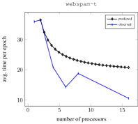
Figure 2: The average time per epoch using $p$ machines on the webspam-t dataset.

Algorithms that use so-called parameter server to synchronize variable updates across processors have recently become popular (e.g., LiAndSmoYu14). The main drawback of these methods is that it is not easy to “serialize” the updates, that is, to replay the updates on a single machine. This makes proving convergence guarantees, and debugging such frameworks rather difficult, although some recent progress has been made [LiAndSmoYu14].

The observation that updates on individual coordinates of the parameters can be carried out in parallel has been used for other models. In the context of Latent Dirichlet Allocation, Yan et al. [30] used a similar observation to derive an efficient GPU based collapsed Gibbs sampler. On the other hand, for matrix factorization Gemulla et al. [10] and Recht and Ré [21] independently proposed parallel algorithms based on a similar idea. However, to the best of our knowledge, rewriting (1) as a saddle point problem in order to discover parallelism is our novel contribution.

5 Experiments

5.1 Scaling

We first verify, that the per epoch complexity of DSO scales as $\left|\Omega\right|T_{\rm u}/p+T_{\rm c}$, as predicted by our analysis in Section 3.1. Towards this end, we took tthe webspam-t dataset of Webb et al. [29], which is one of the largest datasets we could comfortably fit on a single machine. We let $p=\left\{1,2,4,8,16\right\}$ while fixing the number of cores on each machine to be 4.

Using the average time per epoch on one and two machines, one can estimate $\left|\Omega\right|T_{\rm u}$ and $T_{\rm c}$. Given these values, one can then predict the time per iteration for other values of $p$. Figure 2 shows the predicted time and the measured time averaged over 40 epochs. As can be seen, the time per epoch indeed goes down as $\approx 1/p$ as predicted by the theory. The test error and objective function values on multiple machines was very close to the test error and objective function values observed on a single machine, thus confirming Theorem 1.

5.2 Comparison With Other Solvers

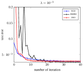
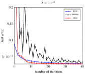
Figure 3: The test error of different optimization algorithms on linear SVM with real-sim dataset, as a function of the number of iteration.

In our single machine experiments we compare DSO with Stochastic Gradient Descent (SGD) and Bundle Methods for Regularized risk Minimization (BMRM) of Teo et al. [28]. In our multi-machine experiments we compare with Parallel Stochastic Gradient Descent (PSGD) of Zinkevich et al. [34] and BMRM. We chose these competitors because, just like DSO, they are general purpose solvers for regularized risk minimization (1), and hence can solve non-smooth problems such as SVMs as well as smooth problems such as logistic regression. Moreover, BMRM is a specialized solver for regularized risk minimization, which has similar performance to other first-order solvers such as ADMM.

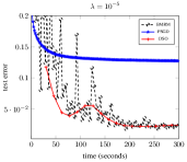
Figure 4: Logistic regression with webspam-t dataset. Test error as a function of elapsed time.

We selected two representative datasets and two values of the regularization parameter $\lambda=\left\{10^{-5},10^{-6}\right\}$ to present our results. For the single machine experiments we used the real-sim dataset from Hsieh et al. [13], while for the multi-machine experiments we used webspam-t. Details of the datasets can be found in Table 1 in the appendix. We use test error rate as comparison metric, since stochastic optimization algorithms are efficient in terms of minimizing generalization error, not training error [3]. The results for single machine experiments on linear SVM training can be found in Figure 3. As can be seen, DSO shows comparable efficiency to that of SGD, and outperforms BMRM. This demonstrates that saddlepoint optimization is a viable strategy even in serial setting.

Our multi-machine experimental results for linear SVM training can be found in Figure 5. As can be seen, PSGD converges very quickly, but the quality of the final solution is poor; this is probably because PSGD only solves processor-local problems and does not have a guarantee to converge to the global optimum. On the other hand, both BMRM and DSO converges to similar quality solutions, and at fairly comparable rates. Similar trends we observed on logistic regression. Therefore we only show the results with $10^{-5}$ in Figure 4.

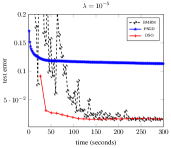
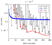
Figure 5: Test errors of different parallel optimization algorithms on linear SVM with webspam-t dataset, as a function of elapsed time.

5.3 Terascale Learning with DSO

Next, we demonstrate the scalability of DSO on one of the largest publicly available datasets. Following the same experimental setup as Agarwal et al. [1], we work with the splice site recognition dataset [27] which contains 50 million training data points, each of which has around 11.7 million dimensions. Each datapoint has approximately 2000 non-zero coordinates and the entire dataset requires around 3 TB of storage. Previously [27], it has been shown that sub-sampling reduces performance, and therefore we need to use the entire dataset for training.

Similar to Agarwal et al. [1], our goal is not to show the best classification accuracy on this data (this is best left to domain experts and feature designers). Instead, we wish to demonstrate the scalability of DSO and establish that a) it can scale to such massive datasets, and b) the empirical performance as measured by AUPRC (Area Under Precision-Recall Curve) improves as a function of time.

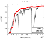
Figure 6: AUPRC (Area Under Precision-Recall Curve) as a function of elapsed time on linear SVM with splice site recognition dataset.

We used 14 machines with 8 cores per machine to train a linear SVM, and plot AUPRC as a function of time in Figure 6. Since PSGD did not perform well in earlier experiments, here we restrict our comparison to BMRM. This experiment demonstrates one of the advantages of stochastic optimization, namely that the test performance increases steadily as a function of the number of iterations. On the other hand, for a batch solver like BMRM the AUPRC fluctuates as a function of the iteration number. The practical consequence of this observation is that, one usually needs to wait for a batch optimizer to converge before using the resulting solution. On the other hand, even the partial solutions produced by a stochastic optimizer such as DSO usually exhibit good generalization properties.

6 Discussion and Conclusion

We presented a new reformulation of regularized risk minimization as a saddle point problem, and showed that one can derive an efficient distributed stochastic optimizer (DSO). We also proved rates of convergence of DSO. Unlike other solvers, our algorithm does not require strong convexity and thus has wider applicability. Our experimental results show that DSO is competitive with state-of-the-art optimizers such as BMRM and SGD, and outperforms simple parallel stochastic optimization algorithms such as PSGD.

A natural next step is to derive an asynchronous version of DSO algorithm along the lines of the NOMAD algorithm proposed by Yun et al. [32]. We believe that our convergence proof which only relies on having an equivalent serial sequence of updates will still apply. Of course, there is also more room to further improve the performance of DSO by deriving better step size adaptation schedules, and exploiting memory caching to speed up random access.

Appendix A Dataset and Implementation Details

Table 1: Summary of the datasets used in our experiments. $m$ is the total # of examples, $d$ is the # of features, $s$ is the feature density (% of features that are non-zero). K/M/G denotes a thousand/million/billion.

Name	$m$.aa	$d$aaa	$\left|\Omega\right|$	$s$(%)
real-sim	57.76K	20.95K	2.97M	0.245
webspam-t	350.00K	16.61M	1.28G	0.022

We implemented DSO, SGD, and PSGD ourselves, while for BMRM we used the optimized implementation that is available from the toolkit for advanced optimization (TAO)(https://bitbucket.org/sarich/tao-2.2). All algorithms are implemented in C++ and use MPI for communication. In our multi-machine experiments, each algorithm was run on four machines with eight cores per machine. DSO, SGD, and PSGD used AdaGrad [8] step size adaptation. We also used Stochastic Variance Reduced Gradient (SVRG) of Johnson and Zhang [15] to accelerate updates of DSO. In the multi-machine setting DSO initializes parameters of each MPI process by locally executing twenty iterations of dual coordinate descent [9] on its local data to locally initialize $w_{j}$ and $\alpha_{i}$ parameters; then $w_{j}$ values were averaged across machines. We chose binary logistic regression and SVM as test problems, i.e., $\phi_{j}(s)=\frac{1}{2}s^{2}$ and $\ell_{i}(u)=\log(1+\exp(-u)),[1-u]_{+}$. To prevent degeneracy in logistic regression, values of $\alpha_{i}$’s are restricted to $(10^{-14},1-10^{-14})$, while in the case of linear SVM they are restricted to $[0,1]$. Similarly, the $w_{j}$’s are restricted to lie in the interval $[-1/\sqrt{\lambda},1/\sqrt{\lambda}]$ for linear SVM and $[-\sqrt{\log(2)/\lambda},\sqrt{\log(2)/\lambda}]$ for logistic regression, following the idea of Shalev-Shwartz et al. [25].

Appendix B Proofs

Let $\left(\mathbf{w}^{t},\bm{\alpha}^{t}\right)$ denote the parameter vector after the $t$-th epoch. Without loss of generality, we will focus on the inner iterations of the $\left(t+1\right)$-st epoch. Consider a time instance at which $k$ updates corresponding to $\left(i_{1},j_{1}\right),\left(i_{2},j_{2}\right),\ldots,\left(i_{k},j_{k}\right)$ have been performed on $\left(\mathbf{w}^{t},\bm{\alpha}^{t}\right)$, which results in the parameter values denoted by $\left(\mathbf{w}_{k}^{t},\bm{\alpha}_{k}^{t}\right)$. In terms of analysis, it is useful to recognize that there is a natural ordering of these updates as follows: $\left(i_{a},j_{a}\right)$ appears before $\left(i_{b},j_{b}\right)$ if updates to $\left(w_{j_{a}},\alpha_{i_{a}}\right)$ were performed before updating $\left(w_{j_{b}},\alpha_{i_{b}}\right)$. On the other hand, if $\left(w_{j_{a}},\alpha_{i_{a}}\right)$ and $\left(w_{j_{b}},\alpha_{i_{b}}\right)$ were updated at the same time because we have $p$ processors simultaneously updating the parameters, then the updates are ordered according to the rank of the processor performing the update. The following lemma asserts that the updates are serializable in the sense that $\left(\mathbf{w}^{t}_{k},\bm{\alpha}^{t}_{k}\right)$ can be recovered by performing $k$ serial updates on function $f_{k}$ which is defined below.

Lemma 2.

For all $k$ and $t$ we have

$$\mathbf{w}^{t}_{k}=\mathbf{w}^{t}_{k-1}-\eta_{t}\nabla_{\mathbf{w}}f_{k}\left(\mathbf{w}^{t}_{k-1},\bm{\alpha}^{t}_{k-1}\right)\text{ and }\bm{\alpha}^{t}_{k}=\bm{\alpha}^{t}_{k-1}-\eta_{t}\nabla_{\bm{\alpha}}{-f}_{k}\left(\mathbf{w}^{t}_{k-1},\bm{\alpha}^{t}_{k-1}\right),$$ (11)

where

$$f_{k}(\mathbf{w},\bm{\alpha}):=f_{i_{k},j_{k}}\left(w_{j_{k}},\alpha_{i_{k}}\right).$$

Proof.

Let $q$ be the processor which performed the $k$-th update in the $\left(t+1\right)$-st epoch. Moreover, let $\left(k-\delta\right)$ be the most recent pervious update done by processor $q$. There exists $\delta\geq\delta^{\prime},\delta^{\prime\prime}\geq 1$ such that $\left(\mathbf{w}^{t}_{k-\delta^{\prime}},\bm{\alpha}^{t}_{k-\delta^{\prime\prime}}\right)$ be the parameter values read by the $q$-th processor to the perform $k$-th update. Because of our data partitioning scheme, only $q$ can change the value of the $i_{k}$-th component of $\bm{\alpha}$ and the $j_{k}$-th component of $\mathbf{w}$. Therefore, we have

$$\alpha^{t}_{k-1,i_{k}}=\alpha^{t}_{\kappa,i_{k}},\qquad k-\delta\leq\kappa\leq k-1,$$ (12)

$$w_{k-1,j_{k}}=w^{t}_{\kappa,j_{k}},\qquad k-\delta\leq\kappa\leq k-1.$$ (13)

Since $f_{k}$ is invariant to changes in any coordinate other than $\left(i_{k},j_{k}\right)$, we have

$$f_{k}\left(\mathbf{w}^{t}_{k-\delta^{\prime}},\bm{\alpha}^{t}_{k-\delta^{\prime\prime}}\right)=f_{k}\left(\mathbf{w}^{t}_{k-1},\bm{\alpha}^{t}_{k-1}\right).$$ (14)

The claim holds because we can write the $k$-th update formula as

$$\mathbf{w}^{t}_{k} =\mathbf{w}^{t}_{k-1}-\eta_{t}\nabla_{\mathbf{w}}f_{k}\left(\mathbf{w}^{t}_{k-\delta^{\prime}},\bm{\alpha}^{t}_{k-\delta^{\prime\prime}}\right)\text{ and }$$ (15)

$$\bm{\alpha}^{t}_{k} =\bm{\alpha}^{t}_{k-1}-\eta_{t}\nabla_{\bm{\alpha}}{-f}_{k}\left(\mathbf{w}^{t}_{k-\delta^{\prime}},\bm{\alpha}^{t}_{k-\delta^{\prime\prime}}\right).$$ (16)

∎

As a consequence of the above lemma, it suffices to analyze the serial convergence of the function $f(\mathbf{w},\bm{\alpha}):=\sum_{k}f_{k}(\mathbf{w},\bm{\alpha})$. Towards this end, we first prove the following technical lemma. Note that it is closely related to general results on convex functions ( e.g., Theorem 3.2.2 in [20], Lemma 14. 1. in [24] ).

Lemma 3.

Suppose there exists $C>0$ and $D>0$ such that for all $\left(\mathbf{w},\bm{\alpha}\right)$ and $\left(\mathbf{w}^{\prime},\bm{\alpha}^{\prime}\right)$ we have $\left\|\mathbf{w}-\mathbf{w}^{\prime}\right\|^{2}+\left\|\bm{\alpha}-\bm{\alpha}^{\prime}\right\|^{2}\leq D$, and for all $t=1,\ldots,T$ and all $\left(\mathbf{w},\bm{\alpha}\right)$ we have

$$\left\|\mathbf{w}^{t+1}-\mathbf{w}\right\|^{2}+\left\|\bm{\alpha}^{t+1}-\bm{\alpha}\right\|^{2}\leq\left\|\mathbf{w}^{t}-\mathbf{w}\right\|^{2}+\left\|\bm{\alpha}^{t}-\bm{\alpha}\right\|^{2}-2\eta_{t}\left(f\left(\mathbf{w}^{t},\bm{\alpha}\right)-f\left(\mathbf{w},\bm{\alpha}^{t}\right)\right)+C\eta_{t}^{2},$$ (17)

then setting $\eta_{t}=\sqrt{\frac{D}{2Ct}}$ ensures that

$$\varepsilon\left(\tilde{\mathbf{w}}^{T},\tilde{\bm{\alpha}}^{T}\right) \leq\sqrt{\frac{2DC}{T}}.$$ (18)

Proof.

Rearrange (17) and divide by $\eta_{t}$ to obtain

$$2\left(f\left(\mathbf{w}^{t},\bm{\alpha}\right)-f\left(\mathbf{w},\bm{\alpha}^{t}\right)\right)\leq\eta_{t}C+\frac{1}{\eta_{t}}\Big{(}\left\|\mathbf{w}^{t}-\mathbf{w}\right\|^{2}+\left\|\bm{\alpha}^{t}-\bm{\alpha}\right\|^{2}-\left\|\mathbf{w}^{t+1}-\mathbf{w}\right\|^{2}-\left\|\bm{\alpha}^{t+1}-\bm{\alpha}\right\|^{2}\Big{)}.$$

Summing the above for $t=1,\ldots,T$ yields

$$2\sum_{t=1}^{T} f\left(\mathbf{w}^{t},\bm{\alpha}\right)-2\sum_{t=1}^{T}f\left(\mathbf{w},\bm{\alpha}^{t}\right)\leq\sum_{t=1}^{T}\eta_{t}C+\frac{1}{\eta_{1}}\left(\left\|\mathbf{w}^{1}-\mathbf{w}\right\|^{2}+\left\|\bm{\alpha}^{1}-\bm{\alpha}\right\|^{2}\right)$$

$$+\sum_{t=2}^{T-1}\left(\frac{1}{\eta_{t+1}}-\frac{1}{\eta_{t}}\right)\left(\left\|\mathbf{w}^{t}-\mathbf{w}\right\|^{2}+\left\|\bm{\alpha}^{t}-\bm{\alpha}\right\|^{2}\right)$$

$$-\frac{1}{\eta_{T}}\left(\left\|\mathbf{w}^{T+1}-\mathbf{w}\right\|^{2}+\left\|\bm{\alpha}^{T+1}-\bm{\alpha}\right\|^{2}\right)$$

$$\leq\sum_{t=1}^{T}\eta_{t}C+\frac{1}{\eta_{1}}D+\sum_{t=2}^{T-1}\left(\frac{1}{\eta_{t+1}}-\frac{1}{\eta_{t}}\right)D$$

$$\leq\sum_{t=1}^{T}\eta_{t}C+\frac{1}{\eta_{T}}D.$$ (19)

Thanks to convexity in $\mathbf{w}$ and concavity in $\bm{\alpha}$

$$f\left(\tilde{\mathbf{w}}^{T},\bm{\alpha}\right)=f\left(\frac{1}{T}\sum_{t=1}^{T}\mathbf{w}^{t},\bm{\alpha}\right)\leq\frac{1}{T}\sum_{t=1}^{T}f\left(\mathbf{w}^{t},\bm{\alpha}\right),\text{ and }$$ (20)

$$-f\left(\mathbf{w},\tilde{\bm{\alpha}}^{T}\right)=-f\left(\mathbf{w},\frac{1}{T}\sum_{t=1}^{T}\bm{\alpha}^{t}\right)\leq\frac{1}{T}\sum_{t=1}^{T}{-f}\left(\mathbf{w},\bm{\alpha}^{t}\right).$$ (21)

Substituting (20) and (21) into (19), and letting $\eta_{t}=\sqrt{\frac{D}{2Ct}}$ leads to the following sequence of inequalities

$$f\left(\tilde{\mathbf{w}}^{T},\bm{\alpha}\right)-f\left(\mathbf{w},\tilde{\bm{\alpha}}^{T}\right)\leq\frac{\sum_{t=1}^{T}\eta_{t}C+\frac{1}{\eta_{T}}D}{2T}\leq\frac{\sqrt{DC}}{2T}\sum_{t=1}^{T}\frac{1}{\sqrt{2t}}+\sqrt{\frac{DC}{2T}}.$$

The claim in (18) follows by using $\sum_{t=1}^{T}\frac{1}{\sqrt{2t}}\leq\sqrt{2T}$. ∎

To prove convergence of DSO it suffices to show that it satisfies (17). In order to derive (9), $C$ of (17) has to be the order of $d$. In case of $L_{2}$-regularizer, it has to be dependent only on $c$ to obtain (10). The proof is related to techniques outlined in Nedić and Bertsekas [18].

Lemma 4.

Under the assumptions outlined in Theorem 1, Algorithm 1 satisfies (17) with $C$ of the form of $C=C_{1}d$. It does with $C=C_{2}$ in case of $L_{2}$-regularizer. Here $C_{1}$ and $C_{2}$ is dependent only on $c$.

Proof.

For $\mathbf{w}$,

$$\left\|\mathbf{w}_{k}^{t}-\mathbf{w}\right\|^{2} =\left\|\mathbf{w}_{k-1}^{t}-\eta_{t}\nabla_{\mathbf{w}}f_{k}\left(\mathbf{w}_{k-1}^{t},\bm{\alpha}_{k-1}^{t}\right)-\mathbf{w}\right\|^{2}$$

$$=\left\|\mathbf{w}_{k-1}^{t}-\mathbf{w}\right\|^{2}-2\eta_{t}\left\langle\nabla_{\mathbf{w}}f_{k}\left(\mathbf{w}_{k-1}^{t},\bm{\alpha}_{k-1}^{t}\right),\mathbf{w}_{k-1}^{t}-\mathbf{w}\right\rangle+\eta_{t}^{2}\left\|\nabla_{\mathbf{w}}f_{k}\left(\mathbf{w}_{k-1}^{t},\bm{\alpha}_{k-1}^{t}\right)\right\|^{2}$$

$$\leq\left\|\mathbf{w}_{k-1}^{t}-\mathbf{w}\right\|^{2}-2\eta_{t}\left(f_{k}\left(\mathbf{w}_{k-1}^{t},\bm{\alpha}_{k-1}^{t}\right)-f_{k}\left(\mathbf{w},\bm{\alpha}_{k-1}^{t}\right)\right)+\eta_{t}^{2}\left\|\nabla_{\mathbf{w}}f_{k}\left(\mathbf{w}_{k-1}^{t},\bm{\alpha}_{k-1}^{t}\right)\right\|^{2}.$$

Analogously for $\bm{\alpha}$ we have

$$\left\|\bm{\alpha}_{k}^{t}-\bm{\alpha}\right\|^{2} \leq\left\|\bm{\alpha}_{k-1}^{t}-\bm{\alpha}\right\|^{2}-2\eta_{t}\left(-f_{k}\left(\mathbf{w}_{k-1}^{t},\bm{\alpha}_{k-1}^{t}\right)+f_{k}\left(\mathbf{w}_{k-1}^{t},\bm{\alpha}\right)\right)+\eta_{t}^{2}\left\|\nabla_{\mathbf{\bm{\alpha}}}{-f}_{k}\left(\mathbf{w}_{k-1}^{t},\bm{\alpha}_{k-1}^{t}\right)\right\|^{2}.$$

Adding the above two inequalities, rearranging

$$\left\|\mathbf{w}_{k}^{t}-\mathbf{w}\right\|^{2}+\left\|\bm{\alpha}_{k}^{t}-\bm{\alpha}\right\|^{2}-\left\|\mathbf{w}_{k-1}^{t}-\mathbf{w}\right\|^{2}-\left\|\bm{\alpha}_{k-1}^{t}-\bm{\alpha}\right\|^{2}\leq -2\eta_{t}\left(f_{k}\left(\mathbf{w}_{k-1}^{t},\bm{\alpha}\right)-f_{k}\left(\mathbf{w},\bm{\alpha}_{k-1}^{t}\right)\right)$$

$$+\eta_{t}^{2}\left\|\nabla_{\mathbf{w}}f_{k}\left(\mathbf{w}_{k-1}^{t},\bm{\alpha}_{k-1}^{t}\right)\right\|^{2}$$

$$+\eta_{t}^{2}\left\|\nabla_{\mathbf{\bm{\alpha}}}{-f}_{k}\left(\mathbf{w}_{k-1}^{t},\bm{\alpha}_{k-1}^{t}\right)\right\|^{2},$$

and summing the above equation for $k=1,\ldots,\left|\Omega\right|$ obtains

$$\left\|\mathbf{w}^{t+1}-\mathbf{w}\right\|^{2}+\left\|\bm{\alpha}^{t+1}-\bm{\alpha}\right\|^{2}-\left\|\mathbf{w}^{t}-\mathbf{w}\right\|^{2}-\left\|\bm{\alpha}^{t}-\bm{\alpha}\right\|^{2}$$

$$\leq -2\eta_{t}\left(f(\mathbf{w}^{t},\bm{\alpha})-f\left(\mathbf{w},\bm{\alpha}^{t}\right)\right)$$

$$+2\eta_{t}\sum_{k}\left(\left(-f_{k}\left(\mathbf{w},\bm{\alpha}^{t}\right)\right)-\left(-f_{k}\left(\mathbf{w},\bm{\alpha}^{t}_{k-1}\right)\right)\right)$$ (22)

$$+\eta_{t}^{2}\sum_{k}\left\|\nabla_{\mathbf{\bm{\alpha}}}f_{k}\left(\mathbf{w}_{k-1}^{t},\bm{\alpha}_{k-1}^{t}\right)\right\|^{2}$$ (23)

$$+2\eta_{t}\left(\sum_{k}f_{k}\left(\mathbf{w}^{t},\bm{\alpha}\right)-f_{k}\left(\mathbf{w}^{t}_{k-1},\bm{\alpha}\right)+\frac{1}{2}\eta_{t}\left\|\nabla_{\mathbf{w}}f_{k}\left(\mathbf{w}_{k-1}^{t},\bm{\alpha}_{k-1}^{t}\right)\right\|^{2}\right).$$ (24)

In the following, we derive upper bounds for each term of (22), (23) and (24). First observe that

$$\left({-f}_{k}\left(\mathbf{w},\bm{\alpha}^{t}\right)\right)-\left({-f}_{k}\left(\mathbf{w},\bm{\alpha}^{t}_{k-1}\right)\right) \leq\left\langle\nabla_{\mathbf{\bm{\alpha}}}{-f}_{k}(\mathbf{w},\bm{\alpha}^{t}),\bm{\alpha}^{t}_{k-1}-\bm{\alpha}^{t}\right\rangle$$ (25)

$$=\left\langle\nabla_{\mathbf{\bm{\alpha}}}{-f}_{k}(\mathbf{w},\bm{\alpha}^{t}),\sum_{l:l<k-1}\eta_{t}\nabla_{\mathbf{\bm{\alpha}}}{-f}_{l}(\mathbf{w}^{t}_{l-1},\bm{\alpha}^{t}_{l-1})\right\rangle$$ (26)

$$\leq\left\|\nabla_{\mathbf{\bm{\alpha}}}{-f}_{k}(\mathbf{w},\bm{\alpha}^{t})\right\|\left\|\sum_{l:l<k-1,i_{l}=i_{k}}\eta_{t}\nabla_{\mathbf{\bm{\alpha}}}{-f}_{l}(\mathbf{w}^{t}_{l-1},\bm{\alpha}^{t}_{l-1})\right\|.$$ (27)

As we can see

$$\left\|\nabla_{\mathbf{\bm{\alpha}}}{-f}_{k}(\mathbf{w},\bm{\alpha}^{t})\right\| \leq\frac{c}{m\left|\Omega_{i_{k}}\right|}+\frac{\left|w^{t}_{k,j_{k}}x_{i_{k},j_{k}}\right|}{m}$$ (28)

$$\leq\frac{c}{m}\left(\frac{1}{\left|\Omega_{i_{k}}\right|}+\left|x_{i_{k},j_{k}}\right|\right),$$ (29)

using (28), we have

$$\sum_{k}\left\|\nabla_{\mathbf{\bm{\alpha}}}{-f}_{k}(\mathbf{w},\bm{\alpha}^{t})\right\|\leq c+\frac{1}{m}\sum_{i=1}^{m}\sum_{j=1}^{d}\left|w_{j}x_{ij}\right|\leq c+\frac{1}{m}\sum_{i=1}^{m}\left\|\mathbf{\bm{w}}\right\|\left\|\mathbf{\bm{x}}_{i}\right\|\leq 2c^{2}.$$ (30)

On the other hand, using (29), we have

$$\left\|\sum_{l:l<k-1,i_{l}=i_{k}}\eta_{t}\nabla_{\mathbf{\bm{\alpha}}}{-f}_{l}(\mathbf{w}^{t}_{l-1},\bm{\alpha}^{t}_{l-1})\right\| \leq\frac{c\eta_{t}}{m}\left(1+\sum_{j\in\Omega_{i}}\left|x_{ij}\right|\right)$$ (31)

$$\leq\frac{c\eta_{t}}{m}\left(1+\sqrt{\left|\Omega_{i}\right|}\left\|\mathbf{\bm{x}}_{i}\right\|\right)\quad\text{(Cauchy-Schwartz)}$$ (32)

$$\leq\frac{c^{2}\eta_{t}}{m}\left(1+\sqrt{{\max_{i}\left|\Omega_{i}\right|}}\right).$$ (33)

Therefore, we can conclude

$$\sum_{k}\left({-f}_{k}\left(\mathbf{w},\bm{\alpha}^{t}\right)\right)-\left({-f}_{k}\left(\mathbf{w},\bm{\alpha}^{t}_{k-1}\right)\right) =\sum_{k}\left\|\nabla_{\mathbf{\bm{\alpha}}}{-f}_{k}(\mathbf{w},\bm{\alpha}^{t})\right\|\left\|\sum_{l:l<k-1,i_{l}=i_{k}}\eta_{t}\nabla_{\mathbf{\bm{\alpha}}}{-f}_{l}(\mathbf{w}^{t}_{l-1},\bm{\alpha}^{t}_{l-1})\right\|$$ (34)

$$\leq\sum_{k}\left\|\nabla_{\mathbf{\bm{\alpha}}}{-f}_{k}(\mathbf{w},\bm{\alpha}^{t})\right\|\cdot\frac{c^{2}\eta_{t}}{m}\left(1+\sqrt{{\max_{i}\left|\Omega_{i}\right|}}\right)$$ (35)

$$\leq\frac{2c^{4}\eta_{t}^{2}\sqrt{{\max_{i}\left|\Omega_{i}\right|}}}{m}.$$ (36)

Also for the term (23),

$$\sum_{k}\left\|\nabla_{\mathbf{\bm{\alpha}}}{-f}_{k}(\mathbf{w}^{t}_{k-1},\bm{\alpha}^{t}_{k-1})\right\|^{2} \leq\sum_{k}\frac{c^{2}}{m^{2}}\left(\frac{1}{\left|\Omega_{i_{k}}\right|}+\left|x_{i_{k},j_{k}}\right|\right)^{2}$$ (37)

$$\leq\frac{2c^{2}}{m^{2}}\sum_{k}\left(\frac{1}{\left|\Omega_{i_{k}}\right|^{2}}+\left|x_{i_{k},j_{k}}\right|^{2}\right)$$ (38)

$$\leq\frac{2c^{2}}{m^{2}}\sum_{i}\left(\frac{1}{\left|\Omega_{i}\right|}+\left\|\mathbf{x}_{i}\right\|^{2}\right)$$ (39)

$$\leq\frac{4c^{4}}{m}.$$ (40)

Similarly for (24),

$$f_{k}\left(\mathbf{w}^{t},\bm{\alpha}\right)-f_{k}\left(\mathbf{w}_{k-1}^{t},\bm{\alpha}\right) \leq\left\langle\nabla_{\mathbf{w}}f_{k}\left(\mathbf{w}^{t},\bm{\alpha}\right),\mathbf{w}_{k-1}^{t}-\mathbf{w}^{t}\right\rangle$$

$$=\left\langle\nabla_{\mathbf{w}}f_{k}(\mathbf{w}^{t},\bm{\alpha}),\eta_{t}\sum_{l:l<k-1}\nabla_{\mathbf{w}}f_{l}(\mathbf{w}^{t}_{l},\bm{\alpha}^{t}_{l})\right\rangle$$

$$\leq\eta_{t}\sum_{l:l<k-1,j_{l}=j_{k}}\left|\frac{\lambda\nabla\phi(w^{t}_{j_{k}})}{\left|\bar{\Omega}_{j}\right|}-\frac{\alpha_{i_{k}}x_{i_{k},j_{k}}}{m}\right|\left|\frac{\lambda\nabla\phi(w^{t}_{l,j_{l}})}{\left|\bar{\Omega}_{j}\right|}-\frac{\alpha_{i_{l}}x_{i_{l},j_{l}}}{m}\right|$$

$$\leq c^{2}\eta_{t}\sum_{l:l<k-1,j_{l}=j_{k}}\left|\frac{\lambda}{\left|\bar{\Omega}_{j}\right|}+\frac{\left|x_{i_{k},j_{k}}\right|}{m}\right|\left|\frac{\lambda}{\left|\bar{\Omega}_{j}\right|}+\frac{\left|x_{i_{l},j_{l}}\right|}{m}\right|,$$

which leads to

$$f_{k}\left(\mathbf{w}^{t},\bm{\alpha}\right)-f_{k}\left(\mathbf{w}^{t}_{k-1},\bm{\alpha}\right)+\frac{1}{2}\eta_{t}\left\|\nabla_{\mathbf{w}}f_{k}\left(\mathbf{w}_{k-1}^{t},\bm{\alpha}_{k-1}^{t}\right)\right\|^{2}$$ (41)

$$\leq c^{2}\eta_{t}\sum_{l:l<k-1,j_{l}=j_{k}}\left|\frac{\lambda}{\left|\bar{\Omega}_{j}\right|}+\frac{\left|x_{i_{k},j_{k}}\right|}{m}\right|\left|\frac{\lambda}{\left|\bar{\Omega}_{j}\right|}+\frac{\left|x_{i_{l},j_{l}}\right|}{m}\right|+c^{2}\eta_{t}\left|\frac{\lambda}{\left|\bar{\Omega}_{j}\right|}+\frac{\left|x_{i_{k},j_{k}}\right|}{m}\right|\left|\frac{\lambda}{\left|\bar{\Omega}_{j}\right|}+\frac{\left|x_{i_{k},j_{k}}\right|}{m}\right|$$ (42)

$$\leq c^{2}\eta_{t}\sum_{i\in\bar{\Omega}_{j_{k}}}\left|\frac{\lambda}{\left|\bar{\Omega}_{j}\right|}+\frac{\left|x_{i_{k},j_{k}}\right|}{m}\right|\left|\frac{\lambda}{\left|\bar{\Omega}_{j}\right|}+\frac{\left|x_{i,j_{k}}\right|}{m}\right|.$$ (43)

Thus we can get the bound for (24) as follows,

$$\sum_{k}f_{k}\left(\mathbf{w}^{t},\bm{\alpha}\right)-f_{k}\left(\mathbf{w}^{t}_{k-1},\bm{\alpha}\right)+\frac{1}{2}\eta_{t}\left\|\nabla_{\mathbf{w}}f_{k}\left(\mathbf{w}_{k-1}^{t},\bm{\alpha}_{k-1}^{t}\right)\right\|^{2}$$ (44)

$$\leq\sum_{k}c^{2}\eta_{t}\sum_{i\in\bar{\Omega}_{j_{k}}}\left|\frac{\lambda}{\left|\bar{\Omega}_{j}\right|}+\frac{\left|x_{i_{k},j_{k}}\right|}{m}\right|\left|\frac{\lambda}{\left|\bar{\Omega}_{j}\right|}+\frac{\left|x_{i,j_{k}}\right|}{m}\right|$$ (45)

$$=c^{2}\eta_{t}\sum_{j}\sum_{i^{\prime}\in\bar{\Omega}_{j}}\sum_{i\in\bar{\Omega}_{j}}\left|\frac{\lambda}{\left|\bar{\Omega}_{j}\right|}+\frac{\left|x_{i^{\prime},j}\right|}{m}\right|\left|\frac{\lambda}{\left|\bar{\Omega}_{j}\right|}+\frac{\left|x_{i,j}\right|}{m}\right|$$ (46)

$$=c^{2}\eta_{t}\sum_{j}\left(\sum_{i^{\prime}\in\bar{\Omega}_{j}}\left|\frac{\lambda}{\left|\bar{\Omega}_{j}\right|}+\frac{\left|x_{i^{\prime},j}\right|}{m}\right|\right)\left(\sum_{i\in\bar{\Omega}_{j}}\left|\frac{\lambda}{\left|\bar{\Omega}_{j}\right|}+\frac{\left|x_{i,j}\right|}{m}\right|\right)$$ (47)

$$\leq c^{2}\eta_{t}\sum_{j}\left|\bar{\Omega}_{j}\right|\sum_{i\in\bar{\Omega}_{j}}\left|\frac{\lambda}{\left|\bar{\Omega}_{j}\right|}+\frac{\left|x_{i,j}\right|}{m}\right|^{2}$$ (48)

$$\leq 2c^{2}\eta_{t}\sum_{j}\sum_{i\in\bar{\Omega}_{j}}\left(\frac{\lambda^{2}}{\left|\bar{\Omega}_{j}\right|}+\frac{\left|\bar{\Omega}_{j}\right|\left|x_{i,j}\right|^{2}}{m^{2}}\right)$$ (49)

$$\leq 2c^{2}\eta_{t}\sum_{j}\lambda^{2}+2c^{2}\eta_{t}\sum_{i}\sum_{j\in\Omega_{i}}\frac{\left|x_{i,j}\right|^{2}}{m}$$ (50)

$$\leq 2c^{4}d\eta_{t}+2c^{4}\eta_{t}.$$ (51)

Incorporating this bound into (22), (23) and (24), we get

$$\left\|\mathbf{w}^{t+1}-\mathbf{w}\right\|^{2}+\left\|\bm{\alpha}^{t+1}-\bm{\alpha}\right\|^{2}-\left\|\mathbf{w}^{t}-\mathbf{w}\right\|^{2}-\left\|\bm{\alpha}^{t}-\bm{\alpha}\right\|^{2}\leq-2\eta_{t}\left(f\left(\mathbf{w}^{t},\bm{\alpha}\right)-f\left(\mathbf{w},\bm{\alpha}^{t}\right)\right)$$

$$+2\eta_{t}\cdot\left(2c^{4}d\eta_{t}+2c^{4}\eta_{t}\right)+\frac{2c^{4}\eta_{t}^{2}\sqrt{{\max_{i}\left|\Omega_{i}\right|}}}{m}+\frac{4c^{4}}{m}\cdot\eta_{t}^{2}.$$ (52)

Thus we can get such a sufficiently large constant $C$ that $Cd\eta_{t}^{2}$ upper bounds the term of (52).

In the case of $\phi_{j}(s)=\frac{1}{2}s^{2}$, we assume the following additionally $\eta_{t}<\frac{1}{\lambda}$ and $\sqrt{{\max_{i}\left|\Omega_{i}\right|}}<m$. As we can see from the expression (52), assuming $\sqrt{{\max_{i}\left|\Omega_{i}\right|}}<m$, it is sufficient to get the bound for the term (24) which is independent of $d$.

From now on we just write as $i,j$ for $i_{k},j_{k}$ if it is clear from context. The key tool we use is the following bound on $w^{t}_{k-1,j}$. Since $\mathbf{\bm{w}}$ is updated by incremental gradient descent via

$$w^{t}_{k,j}=w^{t}_{k-1,j}-\eta_{t}\left(\frac{\lambda}{\left|\bar{\Omega}_{j}\right|}w^{t}_{k-1,j}-\frac{1}{m}\alpha^{t}_{k-1,i}x_{ij}\right)=\left(1-\frac{\lambda}{\left|\bar{\Omega}_{j}\right|}\eta_{t}\right)w^{t}_{k-1,j}+\frac{1}{m}\eta_{t}\alpha^{t}_{k-1,i}x_{ij}.$$ (53)

Using $\lambda\eta_{t}<1$, we derive

$$\left|w^{t}_{k,j}-w^{t}_{j}\right|\leq\left(1-\left(1-\frac{\lambda}{\left|\bar{\Omega}_{j}\right|}\eta_{t}\right)^{\left|\bar{\Omega}_{j}\right|}\right)\left|w^{t}_{j}\right|+c\eta_{t}v_{j},$$ (54)

where $$v_{j}:=\frac{1}{m}\sum_{i=1}^{m}\left|x_{ij}\right|,\quad\mathbf{\bm{v}}:=(v_{1},\ldots,v_{d})^{\prime}.$$ (55)

The geometric term can be bounded by

$$1-\left(1-\frac{\lambda}{\left|\bar{\Omega}_{j}\right|}\eta_{t}\right)^{\left|\bar{\Omega}_{j}\right|}=\lambda\eta_{t}-\sum_{k=2}^{\left|\bar{\Omega}_{j}\right|}{{\left|\bar{\Omega}_{j}\right|}\choose{k}}\left(\frac{-\lambda}{\left|\bar{\Omega}_{j}\right|}\eta_{t}\right)^{k}\leq\lambda\eta_{t}+(\lambda\eta_{t})^{2}\sum_{k=2}^{\left|\bar{\Omega}_{j}\right|}\frac{1}{k!}\leq c\lambda\eta_{t}.$$ (56)

Therefore we conclude

$$\left|w^{t}_{k,j}-w^{t}_{j}\right|\leq c\eta_{t}(\left|w^{t}_{j}\right|+v_{j}),\qquad\text{and}\qquad\left|w^{t}_{k,j}\right|\leq c\left|w^{t}_{j}\right|+c\eta_{t}v_{j}.$$ (57)

Now we can get

$$\sum_{k}\left\|\nabla_{\mathbf{w}}f_{k}\left(\mathbf{w}_{k-1}^{t},\bm{\alpha}_{k-1}^{t}\right)\right\|^{2} \leq\sum_{k}2\left|\frac{\alpha_{i}}{m}x_{ij}\right|^{2}+2\left|\frac{\lambda}{\left|\bar{\Omega}_{j}\right|}w^{t}_{k-1,j}\right|^{2}$$ (58)

$$\leq\frac{2c^{3}}{m^{2}}\sum_{k}x^{2}_{ij}+\sum_{(i,j)\in\Omega}\frac{2\lambda^{2}}{\left|\bar{\Omega}_{j}\right|^{2}}\left(c\left|w^{t}_{j}\right|+c\eta_{t}v_{j}\right)^{2}$$ (59)

$$\leq\frac{2c^{3}}{m}+\sum_{j}\frac{2c^{2}}{\left|\bar{\Omega}_{j}\right|}\left(c^{2}(w^{t}_{j})^{2}+c^{2}\eta_{t}^{2}v_{j}^{2}\right)$$ (60)

$$\leq\frac{2c^{3}}{m}+2c^{2}(c^{2}\left\|\mathbf{\bm{w}}^{t}\right\|^{2}+c^{2}\eta_{t}^{2}\left\|\mathbf{\bm{v}}\right\|^{2})\leq c_{1},$$ (61)

with a constant $c_{1}$. Also for the rest of the terms in (24), we can see

$$f_{k}\left(\mathbf{w}^{t},\bm{\alpha}\right)-f_{k}\left(\mathbf{w}^{t}_{k-1},\bm{\alpha}\right) =\frac{\lambda}{2\left|\bar{\Omega}_{j}\right|}(w^{t}_{j})^{2}-\frac{\lambda}{2\left|\bar{\Omega}_{j}\right|}(w^{t}_{k-1,j})^{2}-\frac{\alpha_{i}}{m}w^{t}_{j}x_{ij}+\frac{\alpha_{i}}{m}w^{t}_{k-1,j}x_{ij}$$ (62)

$$\leq\left|w^{t}_{k-1,j}-w^{t}_{j}\right|\left(\frac{2c^{2}}{m}\left|x_{ij}\right|+\frac{\lambda}{2\left|\bar{\Omega}_{j}\right|}\left|w^{t}_{k-1,j}+w^{t}_{j}\right|\right)$$ (63)

$$\leq{c\eta_{t}}(\left|w^{t}_{j}\right|+v_{j})\left(\frac{2c^{2}}{m}\left|x_{ij}\right|+\frac{\lambda}{\left|\bar{\Omega}_{j}\right|}(1+c)\left|w^{t}_{j}\right|+\frac{\lambda c}{\left|\bar{\Omega}_{j}\right|}\eta_{t}v_{j}\right)\quad\text{by }\eqref{eq:bound_wt}.$$ (64)

Therefore

$$\sum_{k}f_{k}\left(\mathbf{w}^{t},\bm{\alpha}\right)-f_{k}\left(\mathbf{w}^{t}_{k-1},\bm{\alpha}\right) \leq{2c^{3}\eta_{t}}\sum_{(i,j)\in\Omega}(\left|w^{t}_{j}\right|+v_{j})\left(\frac{1}{m}\left|x_{ij}\right|+\frac{1}{\left|\bar{\Omega}_{j}\right|}\left|w^{t}_{j}\right|+\frac{1}{\left|\bar{\Omega}_{j}\right|}\eta_{t}v_{j}\right)$$ (65)

$$\leq{2c^{3}\eta_{t}}\sum_{j}(\left|w^{t}_{j}\right|+v_{j})\left(\frac{1}{m}\sum_{i=1}^{m}\left|x_{ij}\right|+\left|w^{t}_{j}\right|+\eta_{t}v_{j}\right)$$ (66)

$$\leq{2c^{3}\eta_{t}}(\left\|\mathbf{\bm{w}}^{t}\right\|+\left\|\mathbf{\bm{v}}\right\|)\left(\frac{1}{m}\sum_{i=1}^{m}\left\|\mathbf{\bm{x}}_{i}\right\|+\left\|\mathbf{\bm{w}}^{t}\right\|+\eta_{t}\left\|\mathbf{\bm{v}}\right\|\right)$$ (67)

$$\leq c_{2}\eta_{t},$$ (68)

with a constant $c_{2}$. In the end, we can see, instead of (52), we get

$$\left\|\mathbf{w}^{t+1}-\mathbf{w}\right\|^{2}+\left\|\bm{\alpha}^{t+1}-\bm{\alpha}\right\|^{2}-\left\|\mathbf{w}^{t}-\mathbf{w}\right\|^{2}-\left\|\bm{\alpha}^{t}-\bm{\alpha}\right\|^{2}\leq-2\eta_{t}\left(f\left(\mathbf{w}^{t},\bm{\alpha}\right)-f\left(\mathbf{w},\bm{\alpha}^{t}\right)\right)$$

$$+2\eta_{t}\cdot c_{2}\eta_{t}+c_{1}\eta_{t}^{2}+\frac{c^{4}\eta_{t}^{2}\sqrt{{\max_{i}\left|\Omega_{i}\right|}}}{m}+\frac{4c^{4}}{m}\cdot\eta_{t}^{2}.$$ (69)

Thus we can get such a sufficiently large constant $C$ that $C\eta_{t}^{2}$ upper bounds the term of (69). ∎

References

• Agarwal et al. [2014] A. Agarwal, O. Chapelle, M. Dudík, and J. Langford. A reliable effective terascale linear learning system. JMLR, 15:1111–1133, 2014.
• Bertsekas and Tsitsiklis [1997] D. Bertsekas and J. Tsitsiklis. Parallel and Distributed Computation: Numerical Methods. 1997.
• Bottou and Bousquet [2011] L. Bottou and O. Bousquet. The tradeoffs of large-scale learning. Optimization for Machine Learning, 2011.
• Boyd and Vandenberghe [2004] S. Boyd and L. Vandenberghe. Convex Optimization. 2004.
• Boyd et al. [2010] S. Boyd, N. Parikh, E. Chu, B. Peleato, and J. Eckstein. Distributed optimization and statistical learning via the alternating direction method of multipliers. Found. and Trends in ML, 3(1):1–123, 2010.
• Bradley et al. [2011] J. Bradley, A. Kyrola, D. Bickson, and C. Guestrin. Parallel coordinate descent for L1-regularized loss minimization. In ICML, pages 321–328, 2011.
• Chu et al. [2006] C.-T. Chu, S. K. Kim, Y.-A. Lin, Y. Yu, G. Bradski, A. Y. Ng, and K. Olukotun. Map-reduce for machine learning on multicore. In NIPS, pages 281–288, 2006.
• Duchi et al. [2010] J. Duchi, E. Hazan, and Y. Singer. Adaptive subgradient methods for online learning and stochastic optimization. JMLR, 12:2121–2159, 2010.
• Fan et al. [2008] R.-E. Fan, J.-W. Chang, C.-J. Hsieh, X.-R. Wang, and C.-J. Lin. LIBLINEAR: A library for large linear classification. JMLR, 9:1871–1874, Aug. 2008.
• Gemulla et al. [2011] R. Gemulla, E. Nijkamp, P. J. Haas, and Y. Sismanis. Large-scale matrix factorization with distributed stochastic gradient descent. In KDD, pages 69–77, 2011.
• Hastie et al. [2009] T. Hastie, R. Tibshirani, and J. Friedman. The Elements of Statistical Learning. 2009.
• Ho et al. [2013] Q. Ho, J. Cipar, H. Cui, S. Lee, J. K. Kim, P. B. Gibbons, G. A. Gibson, G. Ganger, and E. P. Xing. More effective distributed ML via a stale synchronous parallel parameter server. In NIPS, 2013.
• Hsieh et al. [2008] C. J. Hsieh, K. W. Chang, C. J. Lin, S. S. Keerthi, and S. Sundararajan. A dual coordinate descent method for large-scale linear SVM. In ICML, pages 408–415, 2008.
• Hsieh et al. [2015] C.-J. Hsieh, H.-F. Yu, and I. S. Dhillon. PASSCoDe: Parallel ASynchronous Stochastic dual Coordinate Descent. In ICML, 2015.
• Johnson and Zhang [2013] R. Johnson and T. Zhang. Accelerating stochastic gradient descent using predictive variance reduction. In NIPS, pages 315–323, 2013.
• Langford et al. [2009] J. Langford, A. J. Smola, and M. Zinkevich. Slow learners are fast. In NIPS, 2009.
• Liu and Nocedal [1989] D. C. Liu and J. Nocedal. On the limited memory BFGS method for large scale optimization. Mathematical Programming, 45(3):503–528, 1989.
• Nedić and Bertsekas [2001] A. Nedić and D. P. Bertsekas. Incremental subgradient methods for nondifferentiable optimization. SIAM Journal on Optimization, 12(1):109–138, 2001.
• Nemirovski et al. [2009] A. Nemirovski, A. Juditsky, G. Lan, and A. Shapiro. Robust stochastic approximation approach to stochastic programming. SIAM J. on Optimization, 19(4):1574–1609, Jan. 2009.
• Nesterov [2004] Y. Nesterov. Introductory Lectures On Convex Optimization: A Basic Course. Springer, 2004.
• Recht and Ré [2013] B. Recht and C. Ré. Parallel stochastic gradient algorithms for large-scale matrix completion. Mathematical Programming Computation, 5(2):201–226, June 2013.
• Recht et al. [2011] B. Recht, C. Re, S. Wright, and F. Niu. Hogwild: A lock-free approach to parallelizing stochastic gradient descent. In NIPS, pages 693–701, 2011.
• Schölkopf and Smola [2002] B. Schölkopf and A. J. Smola. Learning with Kernels. 2002.
• Shalev-Shwartz and Ben-David [2014] S. Shalev-Shwartz and S. Ben-David. Understanding Machine Learning. 2014.
• Shalev-Shwartz et al. [2007] S. Shalev-Shwartz, Y. Singer, and N. Srebro. Pegasos: Primal estimated sub-gradient solver for SVM. In ICML, 2007.
• Smola and Narayanamurthy [2010] A. J. Smola and S. Narayanamurthy. An architecture for parallel topic models. In VLDB, 2010.
• Sonnenburg and Franc [2010] S. Sonnenburg and V. Franc. COFFIN: a computational framework for linear SVMs. In ICML, 2010.
• Teo et al. [2010] C. H. Teo, S. V. N. Vishwanthan, A. J. Smola, and Q. V. Le. Bundle methods for regularized risk minimization. JMLR, 11:311–365, January 2010.
• Webb et al. [2006] S. Webb, J. Caverlee, and C. Pu. Introducing the webb spam corpus: Using email spam to identify web spam automatically. In CEAS, 2006.
• Yan et al. [2009] F. Yan, N. Xu, and Y. Qi. Parallel inference for latent Dirichlet allocation on graphics processing units. In NIPS, pages 2134–2142. 2009.
• Yang [2013] T. Yang. Trading computation for communication: Distributed stochastic dual coordinate ascent. In NIPS, 2013.
• Yun et al. [2014] H. Yun, H.-F. Yu, C.-J. Hsieh, S. V. N. Vishwanathan, and I. S. Dhillon. NOMAD: Non-locking, stOchastic Multi-machine algorithm for Asynchronous and Decentralized matrix completion. VLDB, 2014.
• Zhang and Xiao [2015] Y. Zhang and L. Xiao. DiSCO: Distributed optimization for Self-Concordant empirical loss. In ICML, 2015.
• Zinkevich et al. [2010] M. Zinkevich, A. J. Smola, M. Weimer, and L. Li. Parallelized stochastic gradient descent. In NIPS, pages 2595–2603, 2010.