the Jones polynomial of rational links

Abstract.

We give an explicit formula for the Jones polynomial of any rational link in terms of the denominators of the canonical continued fraction of the slope of the given rational link.

1. Rational links and continued fraction

The class of rational links have been the core of many studies since they have been classified by Schubert in [17] in terms of a rational number called the slope. Many people since then have studied different polynomial invariants of rational links and knots. For example, the authors of [4, 13] give an explicit formula for the Conway (Alexander) polynomial invariant of rational links independently. Moreover, the authors of [3, 6, 10, 11, 12, 14, 15, 18] have studied the Jones polynomial of rational links either directly or indirectly through studying another polynomial invariant that reduces to the Jones polynomial after some special normalization using different techniques.

In this paper, we give an explicit formula for the Jones polynomial of any rational link using a different approach than the one used in the above references. Our approach uses the Kauffman bracket state model given in [8] and its relation to the Tutte polynomial of the Tait graph obtained from the diagram of the given link.

A continued fraction of the rational number $\frac{p}{q}$ is a sequence of integers $b_{1},b_{2},\ldots,b_{n}$ such that

$$\frac{p}{q}=b_{1}+\cfrac{1}{b_{2}+\cfrac{1}{\ldots+\cfrac{1}{b_{n}}}}.$$

This continued fraction of the rational number $\frac{p}{q}$ will be abbreviated by $[b_{1},b_{2},\ldots,b_{n}]$. The integers $b_{i}$ are called the denominators of the continued fraction of the rational number $\frac{p}{q}$.

Each rational link is characterized by a rational number called the slope $\frac{p}{q}$ of a pair of relatively prime integers $p,q$ with $|\frac{p}{q}|\geq 1$ and $q>0$ by the following theorem due to Schubert [17].

Theorem 1.1.

Two rational links $L_{\frac{p}{q}}$ and $L_{\frac{p^{\prime}}{q^{\prime}}}$ are equivalent if and only if

$$p =p^{\prime},$$

$$\text{and }q^{\pm 1} \equiv\pm q^{\prime}(\bmod p).$$

A diagram of a rational link can be constructed from the denominators of any continued fraction of its slope by closing the 4-braid $\sigma_{1}^{b_{1}}\sigma_{2}^{-b_{2}}\sigma_{1}^{b_{3}}\ldots$ in the manner shown in figure 1, where $\sigma_{1},\sigma_{2}$ are shown in figure 2 and the multiplication is defined by concatenating from left to right. It is well known that for odd numerator $p$ this diagram represents a knot and for even numerator $p$ it represents a two component link.

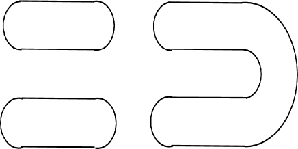
Figure 1. The odd and the even closure of the 4-braid respectively

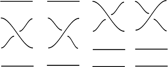
Figure 2. The 4-braids $\sigma_{1},\sigma_{1}^{-1},\sigma_{2},$ and $\sigma_{2}^{-1}$ respectively

It is sufficient to consider the case when the number of denominators of the continued fraction $n$ is odd and $b_{i}\geq 1$ for $i=1,2,\ldots n$ as a result of the following lemma.

Lemma 1.2.

There exists a unique continued fraction of $\frac{p}{q}>1$ of positive integers with $n$ odd and $b_{i}\geq 1$ for $i=1,2,\ldots n$.

Proof.

We start with the rational number $\frac{p}{q}>1$ such that $\gcd(p,q)=1$ and $p>q>0$. Thus we can apply the Euclidean algorithm to get

$$p =qb_{1}+q_{1}, 0<q_{1}<q$$

$$q =q_{1}b_{2}+q_{2}, 0<q_{2}<q_{1}$$

$$q_{1} =q_{2}b_{3}+q_{3}, 0<q_{3}<q_{2}$$

$$\ \ \vdots$$

$$q_{n-3} =q_{n-2}b_{n-1}+q_{n-1}, 0<q_{n-1}<q_{n-2}$$

$$q_{n-2} =q_{n-1}b_{n}.$$

Now we have

$$\frac{p}{q}=\frac{qb_{1}+q_{1}}{q}=b_{1}+\frac{1}{\frac{q}{{q_{1}}}}=b_{1}+\frac{1}{\frac{q_{1}b_{2}+q_{2}}{{q_{1}}}}=b_{1}+\frac{1}{b_{2}+\frac{q_{1}}{q_{2}}}=\dots=b_{1}+\cfrac{1}{b_{2}+\cfrac{1}{b_{3}+\cfrac{1}{\ddots+\cfrac{1}{b_{n}}}}}.$$

In this way, we get a continued fraction $[b_{1},b_{2},\ldots,b_{n}]$ of $\frac{p}{q}$ with $b_{n}\geq 2$ since $q_{n-1}<q_{n-2}$. Now if $n$ is even then $[b_{1},b_{2},\ldots,b_{n}-1,1]$ is the continued fraction with odd number of denominators. Finally, the uniqueness follows from applying the Euclidean algorithm at every step. ∎

Definition 1.3.

The unique continued fraction obtained using the above lemma will be called the canonical continued fraction of $\frac{p}{q}$ and the diagram obtained from the canonical continued fraction will be called the canonical diagram of the rational link whose slope is $\frac{p}{q}$. It is easy to see that the canonical diagram is alternating.

Remark 1.4.

The motivation of the above definition and lemma is the work of the authors in [9, Section. 2] for rational tangles.

Remark 1.5.

Most of the material of this section appears in [16] with the same title and we include it in here to make this paper more self-contained.

2. The Jones polynomial

The Jones polynomial is an invariant of links that was first defined by V. Jones in [5]. It is a Laurent polynomial in one indeterminant defined on the set of oriented links. There are many approaches to define this invariant, but we choose the approach that will serve our purposes in this paper.

The Jones polynomial of a given link can be computed using the Tutte polynomial of the associated Tait’s graph of the given link diagram. In this paper, we restrict our work to alternating link diagrams. Therefore, the associated Tait’s graph will be a planar graph without signs. Now we recall the definition of the Tutte polynomial of graphs and for further details and more basic reference about this polynomial see [1].

Definition 2.1.

The Tutte polynomial $\chi(G;x,y)\in\mathbb{Z}[x,y]$ of a graph $G$ is defined as follows:

1. If the graph $G$ consists only of the vertex $v$, then $\chi(v)=1$.

2. If the graph $G$ consists only of the edge $e$, then$\chi(e)=x$.

3. If the graph $G$ consists only of the loop $l$, then$\chi(l)=y$.

4. If $G_{1}*G_{2}$ denotes a connected graph consists of two graphs $G_{1}$ and $G_{2}$ having just one vertex in common, then $\chi(G_{1}*G_{2})=\chi(G_{1})\chi(G_{2})$.

5. If $G_{1}\sqcup G_{2}$ is the disjoint union of the two graphs $G_{1}$ and $G_{2}$, then $\chi(G_{1}\sqcup G_{2})=\chi(G_{1})\chi(G_{2})$.

6. If $e$ is an edge which is neither a loop nor a bridge of the graph $G$, then $\chi(G)=\chi(G-e)+\chi(G\backslash e)$ where $G-e$ is the graph obtained be deleting the edge $e$ in $G$ and $G\backslash e$ is the graph obtained by contracting the edge $e$ in $G$.

In a graph $G$ a bridge is an edge whose removal increases the number of components of $G$ and a loop is an edge which has the same vertex as its endpoints.

The way to construct the Tait’s graph of a given alternating link diagram is by using the checkerboard coloring, that is we color the regions of the diagram in $\mathbb{R}^{2}$ into two colors black and white such that regions which share an arc have different colors. We then place a vertex in each black region and associate an edge to each crossing of the link that connects two vertices to obtain the graph $G$. By interchanging black regions with white regions, we obtain the dual graph of $G$.

We quote the following lemma that first appeared in [7].

Lemma 2.2.

If the outside region is white, then the Tait’s graph of the canonical rational link diagram takes the form of graph given in figure 4.

Definition 2.3.

The Tait’s graph corresponding to the the canonical rational link diagram will be called the canonical Tait’s graph of the given rational link.

The Jones polynomial of an oriented link can be expressed via the Tutte polynomial of the Tait’s graph in [1] by the following theorem:

Theorem 2.4.

The Jones polynomial $V_{l}(t)$ of an alternating link $L$ can be obtained from the Tutte polynomial $\chi(G;x,y)$ of the assocaited Tait’s graph $G$ by the following equation:

$$V_{L}(t)=(-1)^{w}t^{\frac{a-b-3w}{4}}\chi(G;-t,-t^{-1})$$

where $a$ is the number of white regions, $b$ is the number of black regions, and $w$ is the writhe of the link diagram.

Definition 2.5.

The writhe of a diagram of an oriented link is the number of the crossings of type $L_{+}$ minus the number of crossings of type $L_{-}$ as given in figure 3.

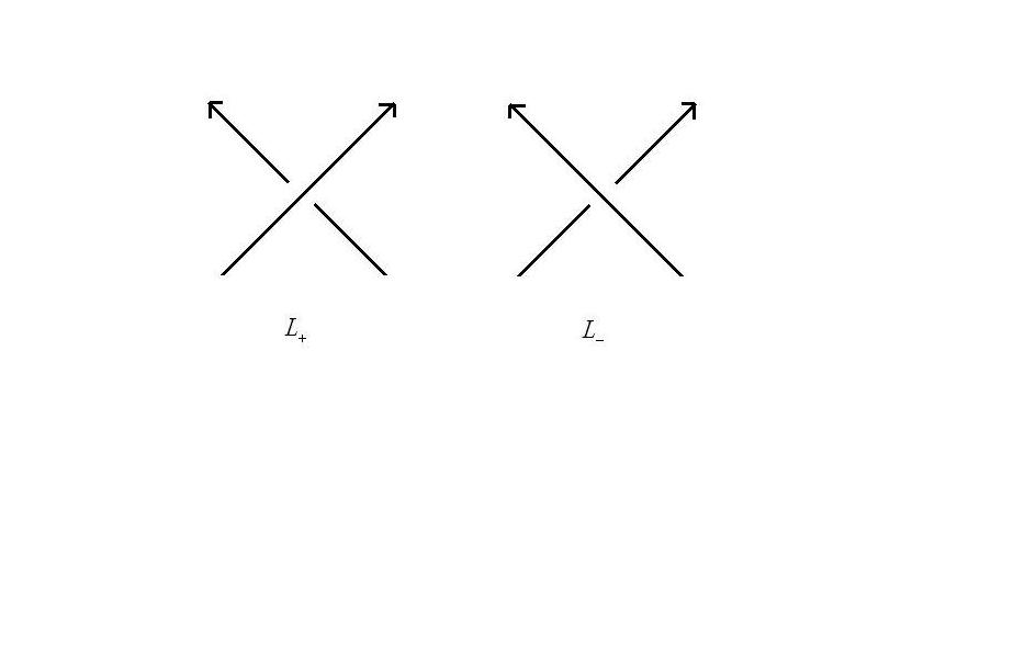
Figure 3. $L_{+}$, and $L_{-}$

3. The Tutte polynomial of the canonical Tait’s Graphs

We give a formula for the Tutte polynomial of the canonical Tait’s graph of any rational link in terms of the denominators of the canonical continued fraction of the slope of the given rational link. First, we recall that a cycle graph of length $p$ is a graph with $p$ vertices and $p$ consecutive edges such that each vertex is incident to two edges.

We quote the following lemmas for later use whose proofs can be found in any basic reference of graph theory see for example [19].

Lemma 3.1.

Let $C_{p}$ be a cycle graph with $p$ edges then the Tutte polynomial is

$$\chi(C_{p})=\frac{x^{p}-1}{x-1}+y-1.$$

Lemma 3.2.

The Tutte polynomial of the dual graph of a graph $G$ equals to the Tutte polynomial of the original graph after interchanging $x$ and $y$.

The canonical Tait’s graph of any rational link is a graph as shown in figure 4 where $b_{i}$ denotes the number of edges that are parallel if $i$ is odd and collinear if $i$ is even with $2+\sum\limits_{i=1}^{k}b_{2i}$ vertices and $\sum\limits_{i=1}^{2k+1}b_{i}$ edges. Let $E=\{b_{2},b_{4},\ldots,b_{2k}\}$, $O=\{b_{1},b_{3},\ldots,b_{2k+1}\}$, $C=\{x:x=\sum\limits_{i=l}^{m}{b_{2i-1}},1\leq l,m\leq k+1\}$ and $\rho(E),\text{ }\rho(C)$ denote the power sets for the sets $E,\text{and }C$ respectively. We define $f:\rho(E)\rightarrow\rho(C)$ by $f(A)=B$, where $x\in B$ iff $x$ is one of the following forms

1. If $A=\phi$, then $x=\sum\limits_{i=1}^{2k+1}b_{i}$.

2. If $b_{l},b_{m}\in A$ and $b_{n}\notin A$ for $l<n<m$, then $x=\underset{l\leq i\leq m,b_{i}\in O}{\sum}b_{i}$.

3. If $b_{m}\in A$ and $b_{n}\notin A$ for $1\leq n<m$, then $x=\underset{1\leq i\leq m,b_{i}\in O}{\sum}b_{i}$.

4. If $b_{l}\in A$ and $b_{n}\notin A$ for $l<n<2k+1$, then $x=\underset{l\leq i\leq 2k+1,b_{i}\in O}{\sum}b_{i}$.

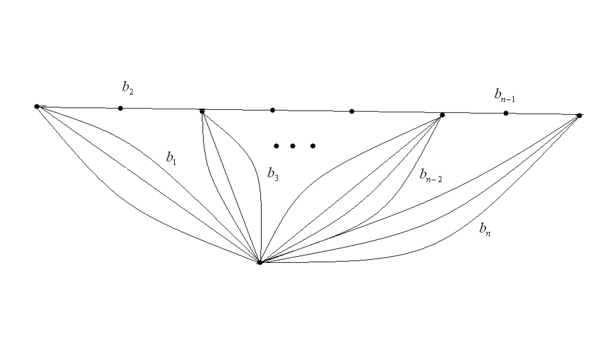
Figure 4. The Graph related to the sequence $\{b_{1},\ldots,b_{n}\}$ of positive integers.

Now, we state the main theorem of this section:

Theorem 3.3.

The Tutte polynomial of the graph shown in figure 4 is given by the formula

$$\chi(G)=\sum_{A\subseteq E}\prod_{{b_{i}}\in A}(\frac{x^{b_{i}}-1}{x-1})\prod_{{\alpha_{i}}\in f(A)}(\frac{y^{\alpha_{i}}-1}{y-1}+x-1).$$

Proof.

We will use induction on $k$. If $k=0$ then $G$ will be the dual graph of $C_{b_{1}}$ so from Lemmas 3.2 and 3.1 we get

$$\chi(G)=\frac{y^{b_{1}}-1}{y-1}+x-1.$$

Now for $k=m$, we apply part 6 of Definition 2.1 on one of the $b_{2k}$-edges that are collinear in figure 4 and use part 4 of the same definition to get

$$\chi(G)=x^{b_{2k}-1}(\frac{y^{b_{2k+1}}-1}{y-1}+x-1)\chi(G^{\prime})+\chi(G^{\prime\prime}),$$

where $G^{\prime},G^{\prime\prime}$ are the canonical Tait’s graphs corresponding to the canonical continued fractions $[b_{1},b_{2},\ldots,b_{2k-1}]$, and $[b_{1},b_{2},\ldots,b_{2k-1},b_{2k}-1,b_{2k+1}]$ respectively. Thus repeating this process $b_{2k}-1$ times on the graph $G^{\prime\prime}$, we obtain

$$\chi(G)=\ (\frac{x^{b_{2k}}-1}{x-1})(\frac{y^{b_{2k+1}}-1}{y-1}+x-1)\chi(G^{\prime})+\chi(G^{\alpha})$$

$$=\ (\frac{x^{b_{2k}}-1}{x-1})(\frac{y^{b_{2k+1}}-1}{y-1}+x-1)\sum_{A\subseteq E^{\prime}}\prod_{{b_{i}}\in A}(\frac{x^{b_{i}}-1}{x-1})\prod_{{\alpha_{i}}\in f(A)}(\frac{y^{\alpha_{i}}-1}{y-1}+x-1)$$

$$\hskip 142.26378pt+\sum_{A\subseteq E^{\alpha}}\prod_{{b_{i}}\in A}(\frac{x^{b_{i}}-1}{x-1})\prod_{{\alpha_{i}}\in f(A)}(\frac{y^{\alpha_{i}}-1}{y-1}+x-1)$$

$$=\ \sum_{A\subseteq E,b_{2k}\in A}\prod_{{b_{i}}\in A}(\frac{x^{b_{i}}-1}{x-1})\prod_{{\alpha_{i}}\in f(A)}(\frac{y^{\alpha_{i}}-1}{y-1}+x-1)$$

$$\hskip 142.26378pt+\sum_{A\subseteq E,b_{2k}\notin A}\prod_{{b_{i}}\in A}(\frac{x^{b_{i}}-1}{x-1})\prod_{{\alpha_{i}}\in f(A)}(\frac{y^{\alpha_{i}}-1}{y-1}+x-1)$$

$$=\ \sum_{A\subseteq E}\prod_{{b_{i}}\in A}(\frac{x^{b_{i}}-1}{x-1})\prod_{{\alpha_{i}}\in f(A)}(\frac{y^{\alpha_{i}}-1}{y-1}+x-1),$$

where $G^{\alpha}$ is the canonical Tait’s graphs corresponding to the canonical continued fraction $[b_{1},b_{2},\ldots,b_{2k-1}+b_{2k+1}]$ and the second equality follows from the induction hypothesis on $G^{\prime}$ and $G^{\alpha}$.

∎

Corollary 3.4.

The Tutte polynomial of the canonical Tait’s graph that corresponds to the rational link $C(b_{1})$ in Conway’s notation in [2] is given by

$$\chi(G;x,y)=\frac{y^{b_{1}}-1}{y-1}+x-1.$$

Proof.

The result follows since the canonical continued fraction the rational link $C(b_{1})$ is $[b_{1}]$ and $E=\{\phi\}$. ∎

Corollary 3.5.

The Tutte polynomial of the canonical Tait’s graph that corresponds to the rational link $C(b_{1},b_{2})$ in Conway’s notation in [2] is given by

$$\chi(G;x,y)=x(\frac{x^{b_{2}-1}-1}{x-1})(\frac{y^{b_{1}}-1}{y-1}+x-1)+\frac{y^{b_{1}+1}-1}{y-1}+x-1.$$

Proof.

The result follows since the canonical continued fraction the rational link $C(b_{1},b_{2})$ is $[b_{1},b_{2}-1,1]$ and $E=\{b_{2}-1\}$. ∎

4. Main Results

For this section, we let $D$ be the canonical link diagram of the rational link $L$ with slope $\frac{p}{q}$ of canonical continued fraction $[b_{1},b_{2},\ldots,b_{n}]$.

We consider the case where $\frac{p}{q}\geq 1$ since the other case yields the mirror image of the link with slope $|\frac{p}{q}|$ and the relation between the Jones polynomial of a link and the Jones polynomial of its mirror image is given by the following theorem:

Theorem 4.1.

Suppose $K^{*}$ is the mirror image of a link $K$, then

$$V_{K^{*}}(t)=V_{K}(t^{-1}).$$

We want to compute the number of white regions, the number of white regions, and the writhe of the canonical diagram $D$ in terms of the denominators of the canonical continued fraction that will be used in the Theorem 4.4.

Lemma 4.2.

Let $G$ be the corresponding Tait’s graph of the canonical diagram $D$, then

$$a =k+1+\sum\limits_{i=1}^{k+1}{(b_{2i-1}-1)}=\sum\limits_{i=1}^{k+1}b_{2i-1}.$$

$$b =|V_{G}|=2+\sum\limits_{i=1}^{k}b_{2i}.$$

We associate to the canonical diagram $D$ a permutation $\sigma_{D}\in S_{3}$ on the set $\{1,2,3\}$. We define the permutation $\sigma_{D}$ in terms of the denominators of the canonical continued fraction by

$$\left(\begin{array}[]{clrr}1&0&0\\ 0&0&1\\ 0&1&0\end{array}\right)^{b_{1}}\left(\begin{array}[]{clrr}0&1&0\\ 1&0&0\\ 0&0&1\end{array}\right)^{b_{2}}\ldots\left(\begin{array}[]{clrr}1&0&0\\ 0&0&1\\ 0&1&0\end{array}\right)^{b_{2k+1}}\left(\begin{array}[]{clrr}1\\ 2\\ 3\end{array}\right)=\left(\begin{array}[]{clrr}\sigma_{D}(1)\\ \sigma_{D}(2)\\ \sigma_{D}(3)\end{array}\right).$$

Now the writhe of the canonical diagram $D$ depends on the permutation $\sigma_{D}$. In particular, we have four cases for the writhe and it is given by the following lemma

Proposition 4.3.

The writhe $w$ of the canonical diagram $D$ is given recursively by

$$w=\begin{cases}b_{1}+b_{2}+\sum\limits_{i=3}^{n}\epsilon_{i}b_{i},&\text{if $\sigma_{D}=(1)$ or $\sigma_{D}=(23)$ or $\sigma_{D}=(12)$ or $\sigma_{D}=(123)$},\\ -b_{1}+b_{2}+\sum\limits_{i=3}^{n}\epsilon_{i}b_{i},&\text{if $(\sigma_{D}=(13)$ or $\sigma_{D}=(132))$ and $b_{1}$ is even},\\ -b_{1}-b_{2}+\sum\limits_{i=3}^{n}\epsilon_{i}b_{i},&\text{if $(\sigma_{D}=(13)$ or $\sigma_{D}=(132))$ and $b_{1}$ is odd},\end{cases}$$

where

$$\epsilon_{i}=\begin{cases}-\epsilon_{i-2},&\text{if $b_{i-1}$ is odd, $i-1$ is even and $\epsilon_{i-1}=1$},\\ -\epsilon_{i-2},&\text{if $b_{i-1}$ is odd, $i-1$ is odd and $\epsilon_{i-1}=-1$ },\\ \epsilon_{i-2},&\text{otherwise}.\end{cases}$$

Proof.

We prove the case where $\sigma_{D}=(23)$. In this case, the canonical diagram $D$ will be closed as in figure 5. We choose the orientation in a way where the top arc always goes from right to left and if the diagram has two components then we can assume the orientation on the bottom arc goes from right to left since these two arcs will belong to different components.

The set of all crossings in the canonical diagram $D$ forms a partition of $n$ elements such that $i$-th element of this partition contains all the crossings that form $\sigma_{1}^{b_{i}}$ if $i$ is odd and $\sigma_{2}^{-b_{i}}$ if $i$ is even in the braid form. It is clear that crossings of the same element of the partition have the same sign. Therefore, we have $w=\sum\limits_{i=1}^{2k+1}\epsilon_{i}b_{i}$. Now after we choose the orientation as above, we obtain $\epsilon_{1}=\epsilon_{2}=1$. Assume that we determine the value of $\epsilon_{i}$ for $1\leq i\leq m-1$ and we want to determine the value of $\epsilon_{m}$. We note that the value of $\epsilon_{m}$ depends on the parity of $b_{m-2},b_{m-1}$ and the values of $\epsilon_{m-2},\epsilon_{m-1}$. Therefore, we can consider the values of $b_{m-2},b_{m-1}$ of being 1 or 2 in the case that $b_{i}$ is odd or even respectively for $i=m-2,m-1$. Now we show one case as in figure 5 and the other cases will be treated similarly. ∎

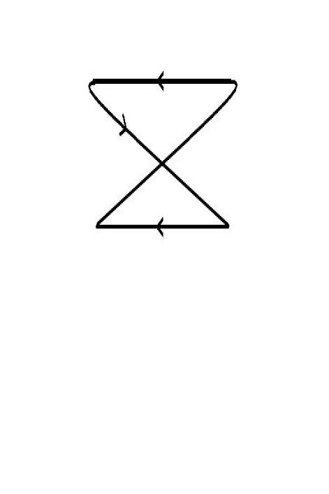
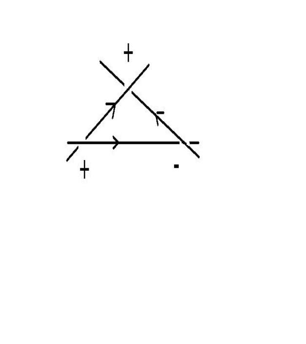
Figure 5. The case where $\sigma_{D}=(23)$ and one of the cases of $\epsilon_{i}$.

From Theorems 3.3, 2.4 and Lemma 4.2, we get a formula of the Jones polynomial of rational links.

Theorem 4.4.

The Jones polynomial of the rational link $L$ with the canonical continued fraction $[b_{1},b_{2},\ldots,b_{2k+1}]$ is

(1) $$V_{L}(t)=(-1)^{w}t^{\frac{\sum\limits_{i=1}^{k+1}b_{2i-1}-(2+\sum\limits_{i=1}^{k}b_{2i})-3w}{4}}\chi(G;-t,-t^{-1}).$$

where $\chi(G;-t,-t^{-1})$ is the Tutte polynomial of the graph $G$ shown in figure 4 computed in Theorem 3.3 and $w$ is the writhe computed in Proposition 4.3.

Corollary 4.5.

The determinant of the rational link $L$ with the canonical continued fraction $[b_{1},b_{2},\ldots,b_{2k+1}]$ is

(2) $$\det(L)=\sum_{A\subseteq E}\prod_{{b_{i}}\in A}b_{i}\prod_{{\alpha_{i}}\in f(A)}\alpha_{i}.$$

Corollary 4.6.

The Jones polynomial of rational link $C(b_{1})$ in Conway’s notation in [2] is given by

$$V_{l}(t)=(-1)^{(b_{1}+1)}t^{\frac{-b_{1}+1}{2}}+\sum\limits_{i=1}^{b_{1}-1}(-1)^{i}(t^{-1})^{\frac{3b_{1}-(2i-1)}{2}}.$$

Proof.

For any rational link with one denominator, we can take an orientation such that $w=b_{1}$. Corollary 3.4 implies

$$\chi(G;-t,-t^{-1})=\frac{(-t^{-1})^{b_{1}}-1}{-t^{-1}-1}-t-1$$

We substitute in equation 1 to get

$$V_{L}(t) =(-1)^{b_{1}}t^{\frac{b_{1}-2-3b_{1}}{4}}(\frac{(-t^{-1})^{b_{1}}-1}{-t^{-1}-1}-t-1)$$

$$=(-1)^{b_{1}}(t^{-1})^{\frac{(b_{1}+1)}{2}}(\sum\limits_{i=1}^{b_{1}-1}(-1)^{b_{1}-i}(t^{-1})^{b_{1}-i}-t)$$

$$=(-1)^{(b_{1}+1)}t^{\frac{-b_{1}+1}{2}}+\sum\limits_{i=1}^{b_{1}-1}(-1)^{i}(t^{-1})^{\frac{3b_{1}-(2i-1)}{2}}.$$

∎

Corollary 4.7.

The Jones polynomial of the rational link $C(b_{1},b_{2})$ in Conway’s notation in [2] is

$$V_{l}(t)=(-1)^{w}t^{\frac{b_{1}-b_{2}-3w}{4}}\left((\frac{(-t)^{b_{2}-1}-1}{-t-1})(\frac{(-t^{-1})^{b_{1}}-1}{-t^{-1}-1}-t-1)(-t)+(\frac{(-t^{-1})^{b_{1}+1}-1}{-t^{-1}-1}-t-1)\right).$$

Proof.

For the rational link with two denominators, we have

$$w=\begin{cases}{b_{1}+b_{2}},&\text{if $b_{1},b_{2}\equiv 1(\bmod 2)$ or $b_{1}\equiv 0(\bmod 2),b_{2}\equiv 1(\bmod 2)$},\\ {-(b_{1}+b_{2})},&\text{if $b_{1}\equiv 1(\bmod 2),b_{2}\equiv 0(\bmod 2)$},\\ {-b_{1}+b_{2}},&\text{if $b_{1},b_{2}\equiv 0(\bmod 2)$}.\end{cases}$$

Corollary 3.5 gives

$$\chi(G;-t,-t^{-1})=-t(\frac{(-t)^{{b_{2}}-1}-1}{-t-1})(\frac{(-t^{-1})^{b_{1}}-1}{-t^{-1}-1}-t-1)+\frac{(-t^{-1})^{b_{1}+1}-1}{-t^{-1}-1}-t-1.$$

Substitute in equation 1 we get

$$V_{l}(t)=(-1)^{w}t^{\frac{b_{1}-b_{2}-3w}{4}}\left((\frac{(-t)^{b_{2}-1}-1}{-t-1})(\frac{(-t^{-1})^{b_{1}}-1}{-t^{-1}-1}-t-1)(-t)+(\frac{(-t^{-1})^{b_{1}+1}-1}{-t^{-1}-1}-t-1)\right).$$

∎

References

- [1] B. Bolloas, Modern Graph Theory, Graduate Texts in Mathematics, vol. 184, Springer-Verlag, New York, 1998.
- [2] J. Conway, An enumeration of knots and links, and some of their algebraic properties, Computational Problems in Abstract Algebra (Proc. Conf., Oxford, 1967), 329–358, Pergamon (1970).
- [3] S. Duzhin, M. Shkolnikov, A formula for the HOMFLY polynomial of rational links, arXiv:1009.1800v2.
- [4] S. Fukuhara, Explicit formula for two-bridge knot polynomials, J. Aust. Math. Soc. 78 (2005), 149-166.
- [5] V. Jones, A polynomial invariant for knots via von Neumann algebras, Bull. Amer. Math. Soc., 12:103-111, 1985.
- [6] T. Kanenobu, Jones and polynomials for 2-bridge knots and links, Proc. Amer. Math. Soc. 110 (3): 835- 841, 1990.
- [7] K. Murasugi, Knot thoery Its Applications, Birkhauser, Boston, 2008.
- [8] L. Kauffman, State models and the Jones polynomial, Topology, 26 (3):395-407, 1987.
- [9] L. Kauffman and S. Lambropoulou, Unknots and Molecular Biology, Milan j. math., 74:227-263, 2006.
- [10] E. Lee, S. Lee, and M. Seo, A Recursive Formula for the Jones Polynomial of 2-bridge Links and Applications, J. Korean Math. Soc. 46 (5) (2009), 919–947 DOI 10.4134/JKMS.2009.46.5.919.
- [11] W. Lickorish and K. Millett, A polynomial invariant of oriented links, Topology 26 (1): 107-141, 1987.
- [12] B. Lu and J. K. Zhong, The Kauffman Polynomials of 2-bridge Knots, arXiv:math. GT/0606114.
- [13] Y. Mizuma, Conway polynomials of two-bridge knots, Kobe J. Math. 21 (2004), 51-60.
- [14] S. Nakabo, Explicit description of the HOMFLY polynomials for 2-bridge knots and links, J. Knot Theory Ramifications 11 (4): 565-574, 2002.
- [15] S. Nakabo, Formulas on the HOMFLY and Jones polynomials of 2-bridge knots and links, Kobe J. of Math. 17 (2000) 131-144.
- [16] K. Qazaqzeh, I. Darabseh, and A. Quraan, The signature of rational links, New York J. Math. 20:183-194, 2014.
- [17] H. Schubert, Knoten mit zwei brucken, Math. Z. 65:133-170, 1956.
- [18] A. Stoimenow, Rational knots and a theorem of Kanenobu, Experiment. Math. 9 (3): 473-478, 2000.
- [19] D. Welsh, The Tutte Polynomial, Random Structures and Algorithms, 15 (3-4):210-228, 1999.