We carefully study the $e\rightarrow m$ and $e\rightarrow 0$ limits of the Reissner-Nordström spacetime using Geroch’s definition of limits of spacetimes. This is implemented by embedding the one-parameter family of spacetimes in anti-de Sitter space, and as a result we obtain metrically correct Penrose diagrams. For $e\rightarrow m$ two distinct limits are studied.

1. Introduction

All students of relativity are familiar with the Reissner-Nordström black hole. Its metric is usually given as

$$ds^{2}=-F(r)dt^{2}+\frac{dr^{2}}{F(r)}+r^{2}(d\theta^{2}+\sin^{2}{\theta}d\phi^{2})\ ,$$ (1)

$$F(r)=1-\frac{2m}{r}+\frac{e^{2}}{r^{2}}\ ,\hskip 22.76219pt0<e^{2}<m^{2}\ .$$ (2)

In the limit $e\rightarrow 0$ this becomes the Schwarzschild metric, and in the limit $e\rightarrow m$ it becomes the metric of an extreme black hole. In both cases large regions of spacetime suddenly disappear. Where did they go?

Even more confusingly, if a simple coordinate transformation is performed first, the metric in the limit $e\rightarrow m$ is not a black hole metric at all. It is the Bertotti-Robinson metric, describing a direct product of 1+1 dimensional anti-de Sitter space with a sphere of constant radius. This geometry also appears in the near-horizon limit of the extremal black hole. So can the extreme black hole be completely bypassed? And are we not told that coordinate changes cannot affect anything?

The student asking such questions is always referred to a classic paper by Geroch [1]. His paper does indeed explain the matter but leaves many details as exercises for the reader. His resolution hinges on one of the core lessons of relativity, namely that there does not exist any canonical way to set up a one-to-one correspondence between the points of the manifolds underlying two different solutions of the field equations. In a situation like the one we are facing (where we want to compare the members of a one-parameter family of spacetimes) the best one can do is to select one point from each member of the family, erect orthonormal frames there, and then regard these points and these frames as “the same”. Only once this has been done can we begin to ask questions about whether a given region in one of these spacetimes has a counterpart in some limit—and the answers will not be forthcoming unless we are willing to solve for the geodesics emerging from that point.

We will give the answers in a new way. The idea is to embed the relevant spacetimes as surfaces in a single embedding spacetime, make sure that they touch tangentially at some chosen point, and then watch how they change as we vary the parameter $e/m$. Three dimensions suffice for the embedding spacetime because it is enough to understand the 1+1 dimensional spacetimes coordinatized by $t$ and $r$. So we will be able to actually see what goes on. (In principle an exactly analogous treatment can be made for the Kerr solution. The results would be similar in many respects, but we would no longer be able to understand them just by looking at a picture because three dimensions no longer suffice for the embedding.)

A few words on embeddings before we begin. Embeddings of spherically symmetric black hole spacetimes in higher dimensional flat spaces have a long history [2], but as far as we know the first actual picture (of the Schwarzschild case) was drawn by Marolf [3]. Embeddings into flat reference spacetimes have been used as tools to investigate various questions of physical interest [4]. Perhaps the one closest in spirit to what we do here is a definition of quasi-local mass, which uses such an embedding to lay the ghost of diffeomorphism invariance to rest [5]. A global embedding was used to elucidate the nature of the Schwarzschild solution [6], but despite some recent progress it is not so easy to embed the Reissner-Nordström spacetime globally in flat space [7]. We take a different route here, and choose anti-de Sitter space as our embedding space. There are two reasons for this. First, it enables us to find an embedding that includes a region large enough for our purposes. Second, in this way we can see what goes on “at infinity” where much of the action is. In effect our pictures share the advantages of Penrose’s conformal diagrams, but they contain all the metric information as well. An obvious drawback is that it takes a certain amount of practice to understand the pictures we draw, but really it is quite a small amount, and we give all the necessary detail in the Appendix.

2. Coordinate calculations

The maximal analytic extension of the Reissner-Nordström spacetime contains an infinite number of regions of three types. We cover one region of each type if we use Eddington-Finkelstein coordinates, in which case the metric is

$$ds^{2}=-F(r)dv^{2}+2dvdr+r^{2}(d\theta^{2}+\sin^{2}{\theta}d\phi^{2})\ ,$$ (3)

$$F(r)=||\partial_{v}||^{2}=\frac{(r-r_{+})(r-r_{-})}{r^{2}}=1-\frac{2m}{r^{2}}+\frac{e^{2}}{r^{2}}\ .$$ (4)

Here $r$ is the area radius of the round 2-spheres and $v$ labels ingoing null geodesics. The roots of the function $F(r)$ are expressed in terms of the mass $m$ and the electric charge $e$ by

$$r_{\pm}=m(1\pm\epsilon)\ ,\hskip 22.76219pt\epsilon=\frac{\sqrt{m^{2}-e^{2}}}{m}\ .$$ (5)

The coordinate system covers a region which is divided into three blocks by Killing horizons associated to the Killing vector field $\partial_{v}$. These blocks are

$$\mbox{I}:\ r>r_{+}\ ,\hskip 17.07164pt\mbox{II}:\ r_{+}>r>r_{-}\ ,\hskip 17.07164pt\mbox{III}:\ r_{-}>r>0\ .$$ (6)

Using a suitable tetrad the only non-vanishing curvature spinors are

$$\Phi_{11^{\prime}}=\frac{e^{2}}{2r^{2}}\ ,\hskip 22.76219pt\Psi_{2}=\frac{e^{2}-mr}{r^{4}}\ .$$ (7)

The first of these determines the traceless Ricci tensor, the second the Weyl tensor. The function $F(r)$ has a minimum at $r=e^{2}/m$, corresponding to a spacelike hypersurface in block II singled out by the fact that $\Psi_{2}$—and hence the Weyl tensor—vanishes there.

In the limit $\epsilon\rightarrow 1$ ($e\rightarrow 0$) block III simply “disappears”. Moreover a singularity develops in block II, so a part of this region disappears as well. If instead we take the limit $\epsilon\rightarrow 0$ ($e\rightarrow m$) we obtain an extreme black hole with a degenerate Killing horizon at $r=m$. Then block II disappears altogether, while the other two blocks “survive”.

But we are free to perform the coordinate change

$$r=m+m\epsilon x\ ,\hskip 22.76219ptv=\frac{m}{\epsilon}u\ .$$ (8)

Then the Reissner-Nordström metric becomes

$$ds^{2}=m^{2}\left[-\frac{(x^{2}-1)}{(1+\epsilon x)^{2}}du^{2}+2dudx+(1+\epsilon x)^{2}(d\theta^{2}+\sin^{2}{\theta}d\phi^{2})\right]\ .$$ (9)

If we now take the limit $\epsilon\rightarrow 0$ ($e\rightarrow m$) we obtain the metric

$$ds^{2}=m^{2}\left[-(x^{2}-1)du^{2}+2dudx+d\theta^{2}+\sin^{2}{\theta}d\phi^{2}\right]\ .$$ (10)

In this limit $\Psi_{2}=0$, so the metric has become conformally flat [8]. It describes a patch of the Bertotti-Robinson spacetime, a direct product of 1+1 dimensional anti-de Sitter space with a sphere of constant radius. All three blocks contribute in this limit.

The story gets an extra twist if we first go to the limit $e=m$ in the original coordinates, then perform the coordinate transformation (8) but this time with a dimensionless parameter $\epsilon$ which is not defined by eq. (5), and finally let this parameter go to zero. The end result is known as the near-horizon geometry of the extremal black hole. Its metric is

$$ds^{2}=m^{2}\left[-x^{2}du^{2}+2dudx+d\theta^{2}+\sin^{2}{\theta}d\phi^{2}\right]\ .$$ (11)

In fact this is the Bertotti-Robinson metric once again, but in a coordinate system covering a different region than that we had above.

Exactly parallel calculations can be made for the Kerr spacetime [9].

3. Geroch’s explanation

Evidently the coordinate calculations are rather confusing, so we turn to Geroch’s paper for clarification. In his setup a one-parameter family of spacetimes is really a five dimensional manifold foliated by the members of the family. The question whether a limit exists is the question whether it is possible to add a boundary to this larger manifold. The reason why a given one-parameter family may admit several different limits can be traced back to the fact that there exists no natural identification point-by-point of two different spacetimes. Any such identification must be added as an extra piece of structure (a vector field) to the five dimensional manifold. Geroch then proves an important rigidity theorem. It says that in order to make the ambiguities go away, we must single out one fiducial point in each spacetime and regard them as (so to speak) the same point, and moreover we must single out one orthonormal tetrad at each such point and regard them as the same tetrad at the same point. The question whether any given point has a counterpart in the limit then turns into the task of finding a broken geodesic connecting the given point to the fiducial point, and studying its behaviour in the limit. This is a well defined procedure because a geodesic from the fiducial point is uniquely determined in terms of the structure we have given, and the tetrad can be parallelly transported along it to determine the remaining segments of the broken geodesic.

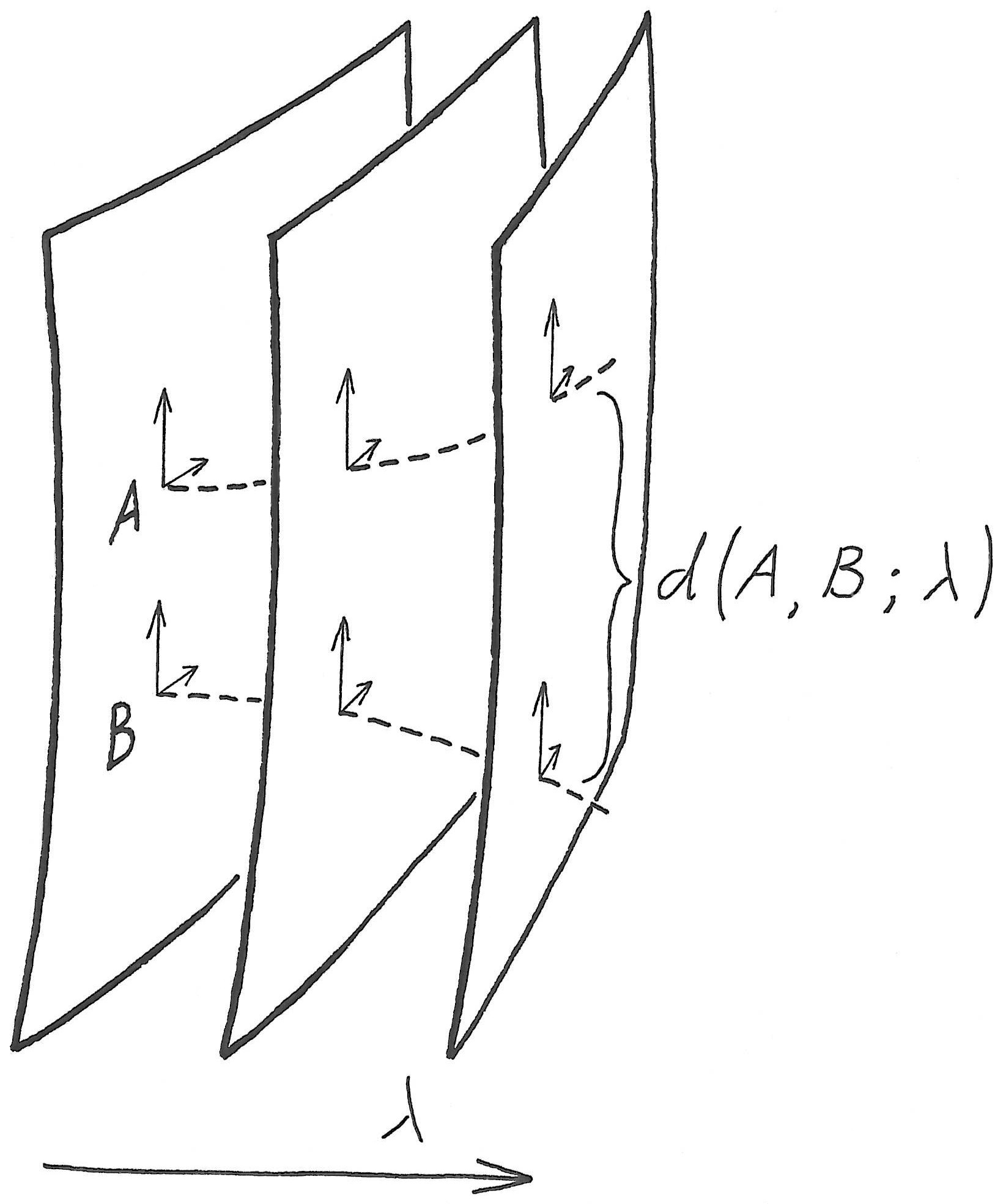
Figure 1: Geroch’s five dimensional manifold is foliated by a family of spacetimes parametrized by a single parameter $\lambda$. We can select points, such as $A$ and $B$, on the leaves and regard them as the same on each leaf. But if the geodesic distance between $A$ and $B$ diverges in the limit they cannot both have counterparts in the same limiting spacetime.

It is now easy to see how different choices of fiducial points can lead to different limits. A glance at Fig. 1 should be enough.

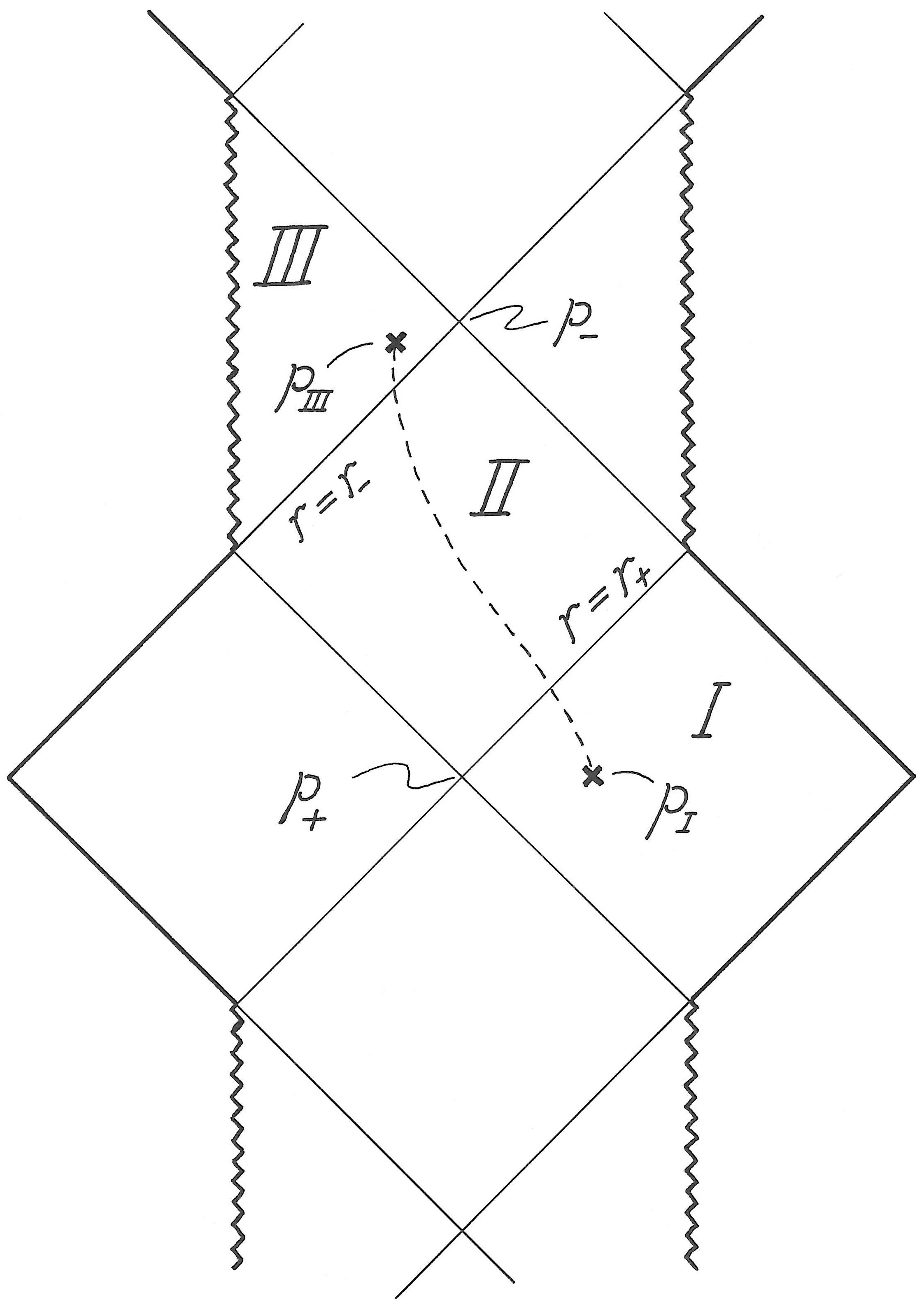
Figure 2: A Penrose diagram of the Reissner-Nordström spacetime. There is an event horizon at $r=r_{+}$ and a Cauchy horizon at $r=r_{-}$. They have bifurcation points $P_{\pm}$. We have also chosen a point $P_{I}$ in the exterior region I and a point $P_{III}$ in the interior region III, since they will play a role in the discussion.

In the case at hand this difficulty does in fact appear. Consider the selection of points in the Reissner-Nordström spacetime that appear in Fig. 2. We can draw geodesics between them (for which purpose the detailed discussion of radial Reissner-Nordström geodesics given by Brigman is helpful [10]). The first observation then is that

$$\lim_{e\rightarrow m}d(P_{+},P_{I})=\infty\ .$$ (12)

This means that at most one of these points can survive in this limit. Similarly

$$\lim_{e\rightarrow m}d(P_{-},P_{III})=\infty\ .$$ (13)

On the other hand

$$d(P_{+},P_{-})=\pi m\ ,$$ (14)

independent of $e$. So we expect that if $P_{+}$ appears in the limit, so does $P_{-}$. This cannot be quite true though, because the point $P_{-}$ does in fact disappear in the $e\rightarrow 0$ limit. We will return to this issue below. A geodesic between $P_{I}$ and $P_{III}$ is naturally divided into three segments, and we are particularly interested in the segment that crosses region II:

$$d(P_{I},P_{III})=d(P_{I},r_{+})+d(r_{+},r_{-})+d(r_{-},P_{III})\ .$$ (15)

For the middle segment we find

$$\lim_{e\rightarrow m}d(r_{+},r_{-})=0\ .$$ (16)

The two points on the horizons will either coincide in the limit, or become null separated. In the former case region II will be absent. If the latter is true something dramatic must happen in the limit to the pair of timelike separated points $P_{I}$ and $P_{III}$—as will become clear later.

Following this line of argument through we recover the two different limits that we encountered in the coordinate calculation. See Fig. 3. Complete understanding requires further calculations. Thus Geroch raises the question how close to the Cauchy horizon a point in region II may come, and still have a counterpart in the Schwarzschild limit $e\rightarrow 0$.

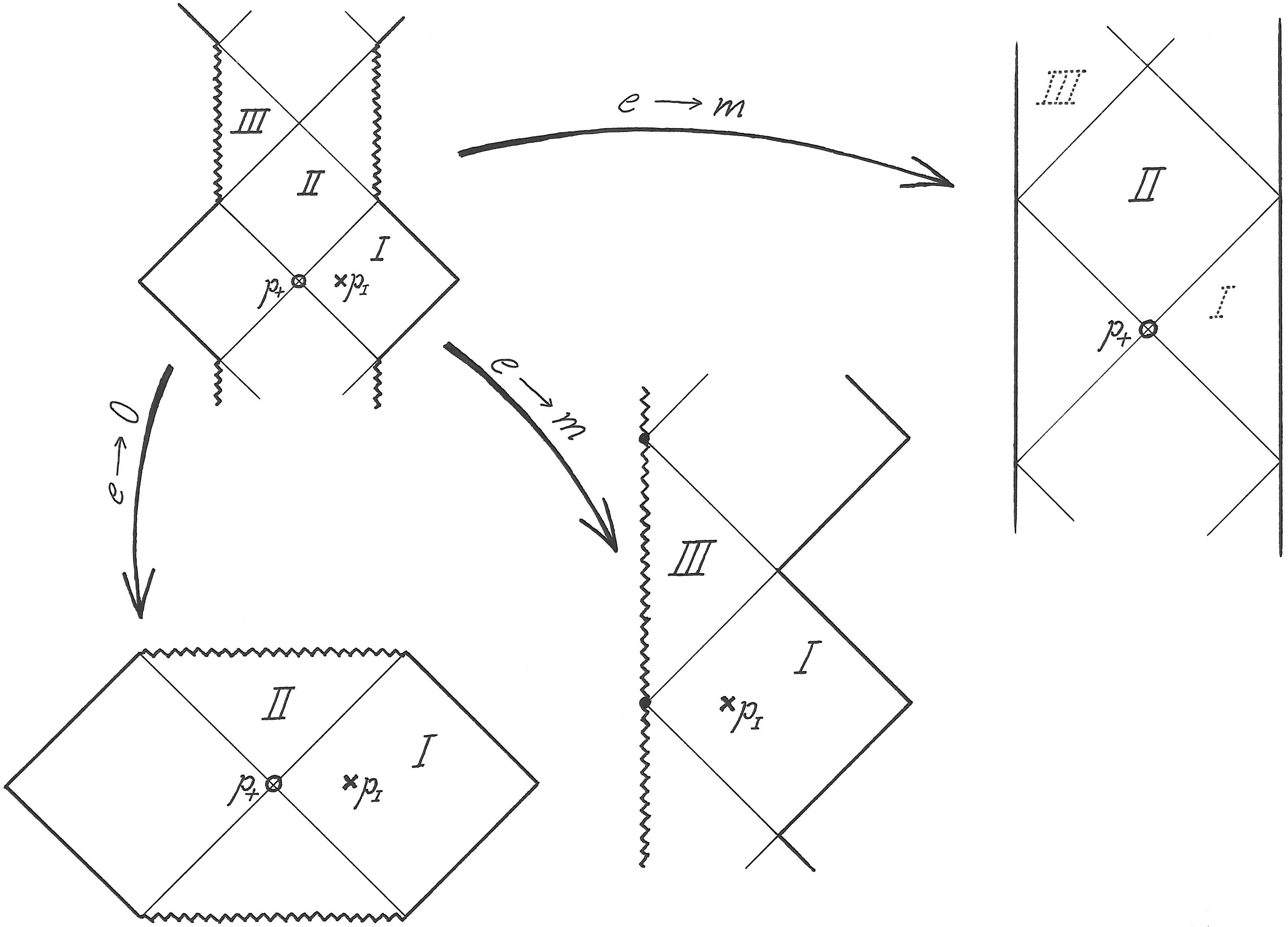
Figure 3: Penrose diagrams of three limiting spacetimes. For the first, $e\rightarrow 0$ and either $P_{+}$ or $P_{I}$ is the preferred point. This is the Schwarzschild spacetime. Region III and a part of region II have disappeared. For the second, $e\rightarrow m$ and $P_{I}$ is the preferred point. This is an extreme black hole. Region II has disappeared. For the third, $e\rightarrow m$ and $P_{+}$ is the preferred point. This is the Bertotti-Robinson spacetime, anti-de Sitter times a sphere. Although there is a region I and a region III in this limit, they are the ghosts of departed quantities in the sense that they come from the near-horizon regions in the original spacetime.

The main purpose of the rest of our paper is to make sure that we really see what goes on—seeing as opposed to just giving nodding agreement to the formulas. Once this has been done it will be easy to answer Geroch’s question, and we do so in section 6.

4. An embedding into anti-de Sitter space

Our way of implementing Geroch’s procedure is to embed all spacetimes into a fixed ambient space. All members of the one-parameter family are to touch at a definite point in this reference space, and moreover their tangent planes are to coincide there. In this way all the requirements for Geroch’s rigidity theorem to hold will be met.

For our purposes it will be enough to embed the 1+1 dimensional spacetimes obtained by ignoring their spherical parts. We will refer to them as black hole surfaces. For our ambient spacetime we choose 2+1 dimensional anti-de Sitter space, trusting that the reader familiarizes herself with the Appendix in order to be able to read the resulting pictures. We choose, quite arbitrarily, the curvature scale $l^{2}=1$ in the ambient space, and as a result our pictures will depend (inessentially but noticeably) on the parameter $m$ that determines the intrinsic spacetime geometry. We will in fact set $m=1$ when drawing the pictures. This represents no loss of generality since we can make the pictures independent of the value of $m$ by adjusting the scale $l^{2}$, although we will not do so explicitly.

For anti-de Sitter space we use the embedding coordinates presented in the Appendix. They are called that because anti-de Sitter space itself is presented as embedded in a flat space of one dimension higher. In the first embedding we place the bifurcation point $P_{+}$ at the point $(X,Y,U,V)=(0,0,0,1)$ for all values of $e$. We refer to this point in anti-de Sitter space as its “origin”, because it serves as the origin of the sausage coordinate system (again we refer to the Appendix).

Explicitly we perform the embedding of the black hole surface by setting

$$Y^{2}-U^{2}=a^{2}F(r)\ ,\hskip 22.76219ptX^{2}-V^{2}=-1-a^{2}F(r)\ .$$ (17)

Here $a$ is a dimensionful constant which will eventually be set equal to $1/\kappa$, where $\kappa$ is the surface gravity of the event horizon. We complete the description by

$$(Y,U)=\left\{\begin{array}[]{cll}a\sqrt{F(r)}(\cosh{\frac{\tau}{a}},\sinh{\frac{\tau}{a}})&\mbox{if}&F(r)>0\\ \\ a\sqrt{-F(r)}(\sinh{\frac{\tau}{a}},\cosh{\frac{\tau}{a}})&\mbox{if}&F(r)<0\end{array}\right.$$ (18)

$$(X,V)=\left\{\begin{array}[]{cll}\sqrt{1+a^{2}F(r)}(\sinh{g},\cosh{g})&\mbox{if}&1+a^{2}F(r)>0\\ \\ \sqrt{-1-a^{2}F(r)}(\cosh{g},\sinh{g})&\mbox{if}&1+a^{2}F(r)<0\ \ .\end{array}\right.$$ (19)

The function $g=g(r)$ is so far undetermined. Some signs still need care since in fact we do not want to restrict ourselves to positive $Y$ when $F(r)>0$ (for instance). By construction $\tau$ is a coordinate along the flow lines of the Killing vector $J_{YU}$. Thus we have identified the static Killing vector field on the black hole surface with the Killing vector $J_{YU}$ in anti-de Sitter space. In this way our construction gains some rigidity.

We still have to choose the form of $g(r)$. We insist that $g(r_{+})=0$. With the above definitions (and a prime to denote derivatives with respect to $r$) the induced metric becomes

$$ds^{2}=dX^{2}+dY^{2}-dU^{2}-dV^{2}=\hskip 128.0374pt$$

(20)

$$=-Fd\tau^{2}+\frac{dr^{2}}{F}\left(F(1+a^{2}F)g^{\prime 2}+\frac{\frac{a^{2}F^{\prime 2}}{4}}{1+a^{2}F}\right)\ .$$

To make this coincide with the metric on the black hole surface—see eq. (1)—we must impose the differential equation

$$g^{\prime 2}=\frac{1+a^{2}F-\frac{a^{2}F^{\prime 2}}{4}}{F(1+a^{2}F)^{2}}\ .$$ (21)

If the right hand side is negative the embedding fails. Since the denominator contains the factor $F(r)$ it changes sign at the horizons, so there is a potential problem with this. We address it by choosing [3]

$$\frac{1}{a}=\kappa=\frac{1}{2}\frac{dF}{dr}_{|r=r_{+}}=\frac{r_{+}-r_{-}}{2r_{+}^{2}}\ .$$ (22)

Thus $\kappa$ is the surface gravity of the outer horizon. This solves the problem because the factor $(r-r_{+})$ cancels out, and the embedding equation becomes

$$g^{\prime 2}=\frac{\kappa^{2}}{4r_{+}^{4}}\frac{(r_{+}-r_{-})^{2}(r^{2}+r_{+}^{2})(r+r_{+})r^{2}+4r_{+}^{4}(r^{4}-r_{+}r_{-})(r-r_{-})}{(r-r_{-})((\kappa^{2}+1)r^{2}-(r_{+}+r_{-})r+r_{+}r_{-})^{2}}\ .$$ (23)

On the right hand side we have a fifth order polynomial divided by another (easily factorized) fifth order polynomial. We see immediately that the denominator changes sign at the inner horizon $r=r_{-}$. Hence we cannot cover both the outer and inner horizons of the black hole surface in this manner. There are two additional zeroes of the denominator between the horizons leading to a divergent but positive expression. This is allowed.

The sign of the numerator at the outer horizon $r=r_{+}$ is easily derived. It is found to be non-negative there whenever

$$r_{+}-r_{-}+r_{+}^{3}-r_{-}\geq 0\ .$$ (24)

In particular it is non-negative whenever $r_{+}^{2}\geq 1$, and this can be arranged for all values of $e^{2}/m^{2}\leq 1$ by choosing $m^{2}\geq 1$. (We remind the reader that the length scale of anti-de Sitter space has already been set equal to one.) If $m$ is so small that $r_{+}^{3}$ can be ignored in comparison to the linear terms the embedding condition at $r=r_{+}$ implies

$$r_{+}\geq 2r_{-}\hskip 14.22636pt\Leftrightarrow\hskip 14.22636pt\frac{e^{2}}{m^{2}}\leq\frac{8}{9}\ .$$ (25)

Because of our choice of a length scale $m<<1$ corresponds to a black hole surface embedded in a nearly flat spacetime, and we conclude—correctly [11]—that a similar embedding into Minkowski space fails when $e^{2}/m^{2}>8/9$. Embedding into anti-de Sitter space is therefore a distinct improvement.

If one really wants to see what happens at the bifurcation point on the inner horizon one can perform another embedding there, but we will not do so here. Our task is to solve the differential equation for $g$, see what the embedded surface looks like, and address the question of limits that is our stated aim.

5. The Schwarzschild surface

Before attending to the details it is helpful to observe that we have arranged the embedding so that the Killing field $J_{YU}$ is everywhere tangential to the surface. In effect then it is enough to determine what the embedding looks like in the Poincaré disk at $t=0$ and in the 1+1 dimensional anti-de Sitter section at $y=0$. (We are slipping into the language of sausage coordinates, which we spell out in the Appendix.) The embedded surface will be swept out from these two curves by the Killing flow lines. The event horizon is a Killing horizon, and will appear as two null geodesics emerging from the origin of anti-de Sitter space.

We begin with the Schwarzschild spacetime ($e=0$), as an exercise. We solve the differential equation (23) using Mathematica, plot the intersection of the embedded black hole surface on the Poincaré disk $t=0$ and on the timelike plane $y=0$, and finally draw the full three-dimensional picture. Of course the result will depend on our choice of the parameter $m$. On the whole the various pictures that we want to draw look nicer if we choose $m=1$, so we settle for this value and show the results in Fig. 4.

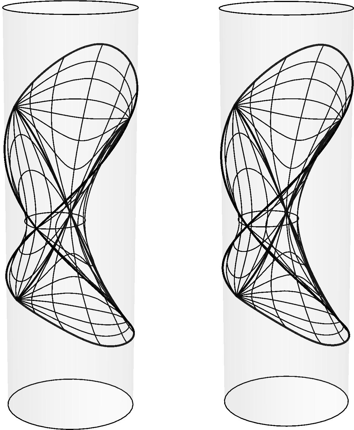
Figure 4: Here is the Schwarzschild surface as a stereogram. The three dimensional picture emerges, in the middle, after appropriate focussing on the part of the reader. The singularity forms a spacelike curve on the anti-de Sitter boundary, and Schwarzschild infinity meets this boundary in a pair of null curves intersecting at $i^{0}$. The event horizon forms two intersecting null geodesics inside the cylinder. For a step by step construction of this surface see Fig. 6.

The picture looks just as one would expect, given that one knows the embedding into flat Minkowski space [3]. A second look is worthwhile though—what we see is a metrically correct Penrose diagram. Its conformal boundaries lie on the anti-de Sitter $\mathscr{I}$ as null lines. In the picture they happen to meet at $i^{0}$, which is not unexpected. The singularity appears as a spacelike curve on $\mathscr{I}$ . At first sight this may seem surprising, since timelike Schwarzschild geodesics can reach it in finite time. However, these curves are not even close to being geodesics in anti-de Sitter space. Indeed it is possible to reach infinity along timelike curves in anti-de Sitter space, and to do so in finite time, provided that one is able to spend rocket fuel at a suitably increasing rate. The same is true in Minkowski space [12].

6. The first two limits of the Reissner-Nordström surface

We now come to the Reissner-Nordström case. Its black hole surface centred at the bifurcation point $P_{+}$ is shown in Fig. 5. However, in order to understand its limits we need to consult Fig. 6, which contains the same information but for a variety of values of $e/m$.

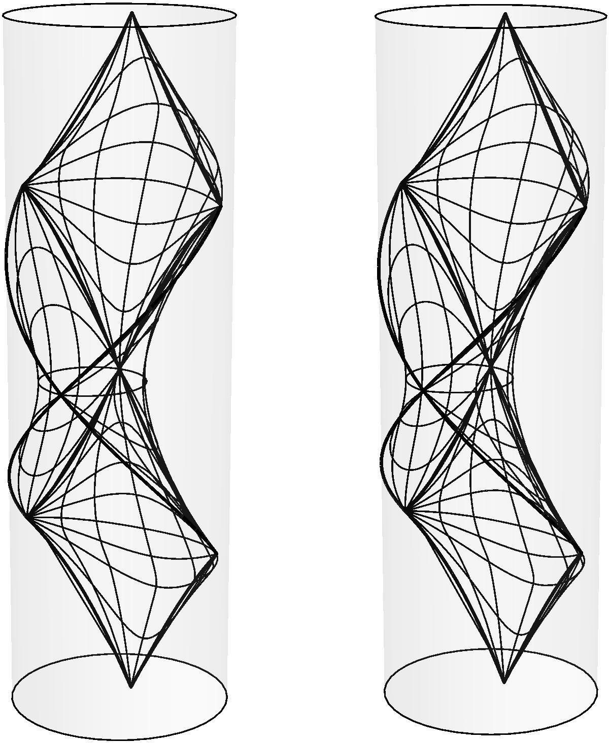
Figure 5: Here is the Reissner-Nordström surface, again as a stereogram, with four blocks of the Penrose diagram included. The embedding fails at the inner horizon, which is seen as two pairs of null geodesics at the top and bottom of the surface. The value of $e/m$ has been set equal to 0.9. Compare to Fig. 6.

Look first at the intersection of the black hole surface with the disk at $t=0$. What we see in Fig. 6 is that it approaches the line $x=0$ as $e\rightarrow m$, and then continues to $i^{0}$ in the immediate vicinity of $\mathscr{I}$ . This means that all points at finite distance from the bifurcation point $P_{+}$ are pushed closer and closer to $\mathscr{I}$. In the picture this is illustrated for a point $P_{I}$ chosen to sit at that value of $r$ for which $r^{2}/F(r)$ has a minimum, which is also that special value of $r$ for which the four dimensional geometry admits a null geodesic at constant $r$. This point sits at a finite distance from the event horizon, but quite close to it in astronomical terms. In the (singular) limit all points originally at finite spacelike distance from $P_{+}$ disappear. Looking next at the intersection with the timelike plane $y=0$ we see that it comes closer and closer to the vertical as $e/m$ increases. In the limit it becomes the vertical. The black hole surface itself tends to the 1+1 dimensional anti-de Sitter space at $x=0$. In this way it becomes clear that the Reissner-Nordström spacetime does indeed approach the Bertotti-Robinson spacetime in the limit $e\rightarrow m$, given that the bifurcation point $P_{+}$ is included in the entire family.

Figure 6: The three dimensional pictures can be understood by looking at the intersection of the surface with the timelike plane at $y=0$ (left; only its upper half is shown) and the disk at $t=0$ (right). Various values of $e/m$ are included. In the plane we have placed a dot at $r=e^{2}/m$ to see where this point is heading as $e\rightarrow 0$. The bend is very sharp, but still smooth, already for $e=0.5m$. In the disk we have marked the point $P_{I}$ (see the text) to see where it goes (namely to infinity) as $e\rightarrow m$. All curves are tangential at the anti-de Sitter origin.

The limit $e\rightarrow 0$ is interesting too, and we can now answer Geroch’s question concerning what points in region II that survive in this limit. In the plane $y=0$ the Reissner-Nordström surface appears as a curve with a bend which will reach $\mathscr{I}$ in the limit $e\rightarrow 0$, and in the limit all points above the bend disappear. The question is then at what $r$-value the bend occurs. Referring back to eq. (19), and noting that $1+a^{2}F<0$ in the interesting region, we see that the bend occurs at

$$X^{\prime}=g^{\prime}\sqrt{-1-a^{2}F(r)}\sinh{g}-\frac{a^{2}F^{\prime}(r)}{2\sqrt{-1-a^{2}F(r)}}\cosh{g}=0\ .$$ (26)

Now keep $r=e^{2}/m$ fixed, so that $F^{\prime}(r)=0$. In fact we place ourselves at the minimum of the function $F$. We know that $F(e^{2}/m)$ diverges in the limit $e\rightarrow 0$. Referring back to eq. (21), and noting that $g$ is finite here, we see that

$$\lim_{e\rightarrow 0}X^{\prime}(e^{2}/m)=\lim_{e\rightarrow 0}\frac{\sinh{g}}{\sqrt{-F(e^{2}/m)}}=0\ .$$ (27)

This locates the position of the bend in the limit, and shows that the surface is discontinued precisely at $r=e^{2}/m$. This then is the answer to the question left open by Geroch.

Incidentally the equation $r=e^{2}/m$ defines a rather interesting hypersurface in the Reissner-Nordström spacetime, since the four dimensional Weyl tensor vanishes there. See eq. (7).

One comment concerning Fig. 6 is that we have to go to rather high values of $e/m$ in order to see any substantial departure from the Schwarzschild case in the vicinity of the bifurcation point $P_{+}$. This is understandable. The principal curvatures $k_{1}$, $k_{2}$ of the embedded surface, which is what one “sees” in the picture, are related to the intrinsic curvature $R$ of the two dimensional black hole surface through the Gauss equation

$$k_{1}k_{2}=1+\frac{R}{2}=1+\frac{2mr-3e^{2}}{r^{4}}\ .$$ (28)

If we set $r=r_{+}$ and then expand in $e/m$ we obtain for the Reissner-Nordström surface that

$$k_{1}k_{2}=1+\frac{1}{4m^{2}}\left(1-\frac{3}{16}\frac{e^{4}}{m^{4}}+\dots\right)\ .$$ (29)

We see that the effects are not noticeable until the number $(e/m)^{4}$ is.

7. The extreme limit of the Reissner-Nordström surface

It remains to recover the other $e\rightarrow m$ limit of the Reissner-Nordström black hole, in which the limit spacetime is an extreme black hole. To do so we focus our attention on a point $P_{I}$ inside region I. We will arrange the embedding in such a way that this point is placed at the origin of anti-de Sitter space. Moreover—in order to ensure that there is a special tetrad attached to that point—we have to do the embedding in such a way that all black hole surfaces meet tangentially there, for all values of $e/m$. This happened almost automatically in our first embedding, but will require conscious effort this time.

The first question is what point to choose. We must make some choice for definiteness, even if it matters only in a rather superficial way. Again we settled for that value of $r$ where the four dimensional geometry admits a null geodesic at constant $r$, namely where $r^{2}/F(r)$ has a minimum. This point (which figures also in the disk shown in Fig. 6) is now to be placed at the anti-de Sitter origin, and all the black hole surfaces are required to meet tangentially there. Then Geroch’s requirements for a well defined limit are met.

Figure 7: A point $P_{I}$ in region I is placed at the anti-de Sitter origin, and all the black hole surfaces meet tangentially there. When we take the limit $e\rightarrow m$ the bifurcation point moves to infinity and an extreme black hole results.

The limiting procedure is illustrated in Fig. 7. We started with a convenient embedding of the extreme black hole surface, and then applied an isometry—in the Poincaré disk, a Möbius transformation—to the previous embeddings, ensuring that all these black hole surfaces have the point $P_{I}$ placed at the anti-de Sitter origin and that they all meet tangentially there. As in the previous case the distance between $P_{I}$ and $P_{+}$ diverges in the limit, but this time it is the bifurcation point $P_{+}$ that is pushed off to infinity.

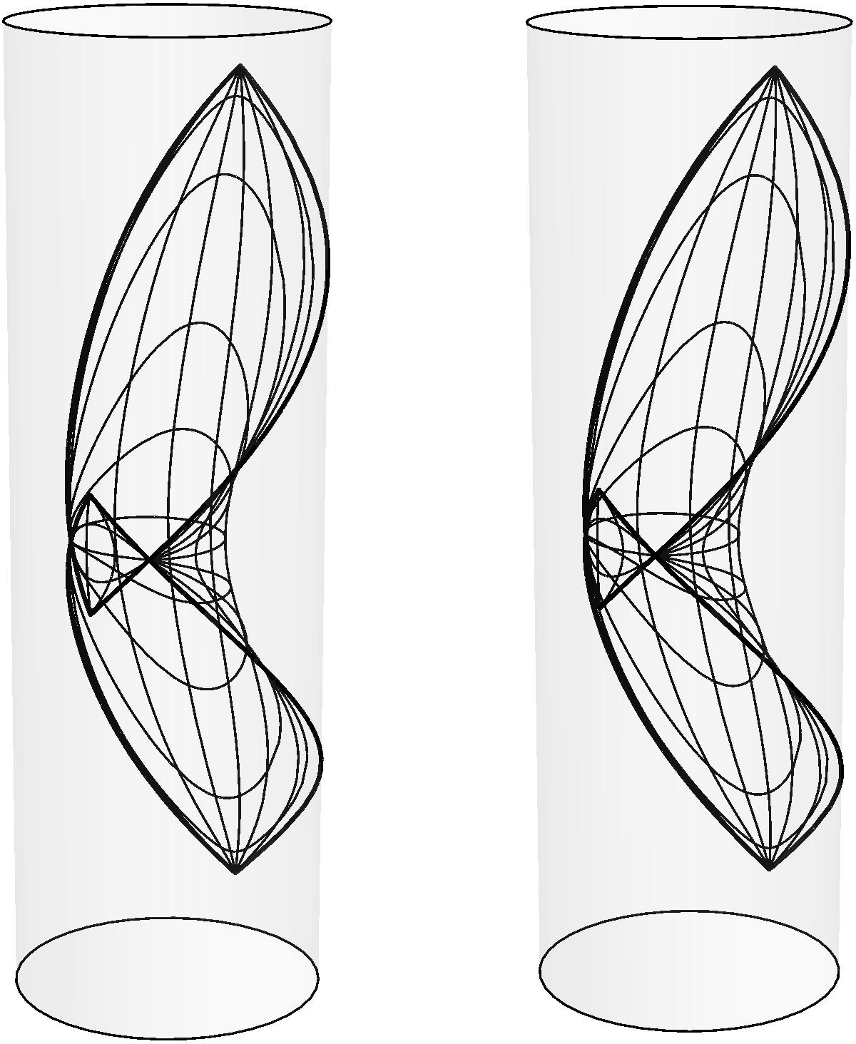
Figure 8: A Reissner-Nordström black hole surface with $e/m=0.9$ and a point $P_{I}$ in its exterior placed at the anti-de Sitter origin. Only its exterior regions are shown, so the surface is bounded by the event horizon. Metrically the two exterior regions have the same size, but one of them sits close to the conformal boundary. The vanishing interior region II is not shown, but if it were, it would be seen that it collapses to a null geodesic connecting two points on $\mathscr{I}$ as $e\to m$.

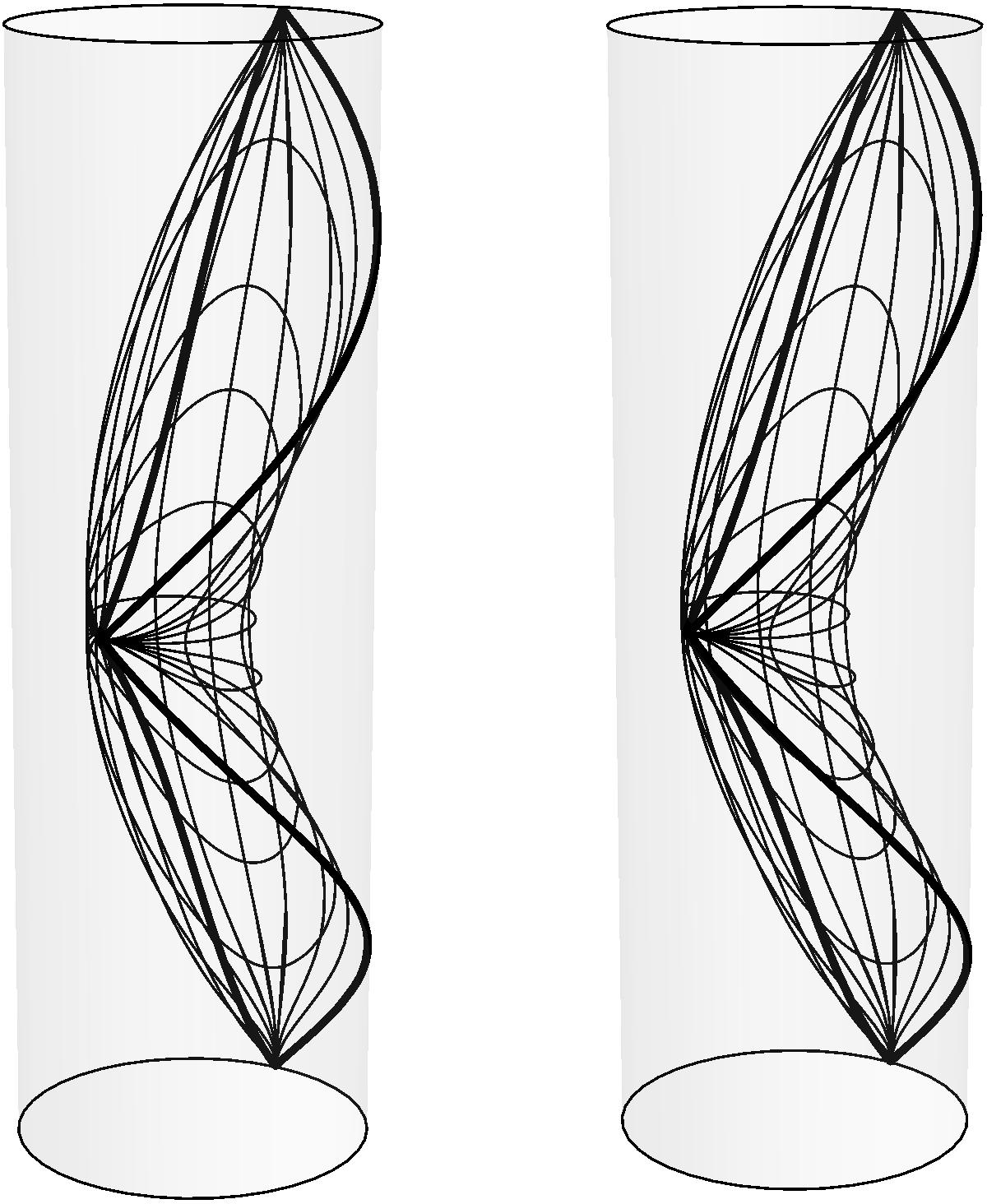
Figure 9: The extreme black hole surface. The embedding does not cover its interior and the horizon is a pair of null geodesics in anti-de Sitter space. Only one exterior region survived the limit.

Stereograms of a Reissner-Nordström black hole arranged in this way, and of the resulting extreme black hole surface, are shown in Figs. 8 - 9. The pictures look skew because the geometry of the extreme black hole is obviously not symmetric under reflection in $P_{I}$. (It does enjoy a discrete conformal symmetry though [13]). Also its Killing vector field is of a different type than that of the non-extreme black hole, when considered as a Killing vector field in anti-de Sitter space. In the terminology of ref. [14] it is type $II_{a}$ rather than type $I_{b}$.

8. Conclusions

We have shown that embeddings into a fixed ambient spacetime can be used to visualize the way a one-parameter family approaches a limiting spacetime. In particular this setting makes transparent the nature of the conditions that Geroch had to impose in order to make such limits well defined, as well as the reasons why a given family of spacetimes may admit several different limits.

Our use of anti-de Sitter space, rather than flat space, as embedding space has the advantages that it becomes simpler to perform the embedding, and that our pictures can be regarded as metrically correct Penrose diagrams. The embedding covers four blocks of the Reissner-Nordström spacetime, which is enough for our purposes.

The reader may have noticed that we have studiously avoided the question whether more than two limiting spacetimes exist (when $e\rightarrow m$). We do not know the answer, but we do know that the possibilites are tightly constrained. The only interesting case where the answer appears to be known is that of the $m\rightarrow\infty$ limits of the Schwarzschild spacetime. There a coordinate free calculation based on the Cartan-Karlhede scalars has shown that five different limits exist [15]. But that method has its drawback too, since it rather obscures the physical nature of the limits. It would be interesting to combine methods.

Acknowledgements: We thank Helgi Rúnarsson, Istvan Racz, José Senovilla, and Stefan Åminneborg for their encouraging interest in limits.

Appendix: Visualizing anti-de Sitter space

A first remark is that visualizing anti-de Sitter is in many ways easier than visualizing Minkowski space, because the conformally compactified version is so much simpler to see.

Sausage coordinates: The standard description of 2+1 dimensional anti-de Sitter space is as the hypersurface

$$X^{2}+Y^{2}-U^{2}-V^{2}=-l^{2}$$ (30)

embedded in a four dimensional space with the indefinite metric

$$ds^{2}=dX^{2}+dY^{2}-dU^{2}-dV^{2}\ .$$ (31)

There is a natural length scale $l$. We set $l=1$ by fiat. The best way to visualize this spacetime is to use the sausage coordinates $(t,x,y)$ defined by

$$X=\frac{2x}{1-\rho^{2}}\hskip 17.07164ptY=\frac{2y}{1-\rho^{2}}\hskip 17.07164ptU=\frac{1+\rho^{2}}{1-\rho^{2}}\sin{t}\hskip 17.07164ptV=\frac{1+\rho^{2}}{1-\rho^{2}}\cos{t}\ ,$$ (32)

where $\rho^{2}=x^{2}+y^{2}<1$. The anti-de Sitter metric is then

$$ds^{2}=-\left(\frac{1+\rho^{2}}{1-\rho^{2}}\right)^{2}dt^{2}+\frac{4}{(1-\rho^{2})^{2}}(dx^{2}+dy^{2})\ .$$ (33)

The resulting picture is that of a solid cylinder, with $\mathscr{I}$ at its boundary and with spatial slices at constant $t$ being copies of the Poincaré disk.

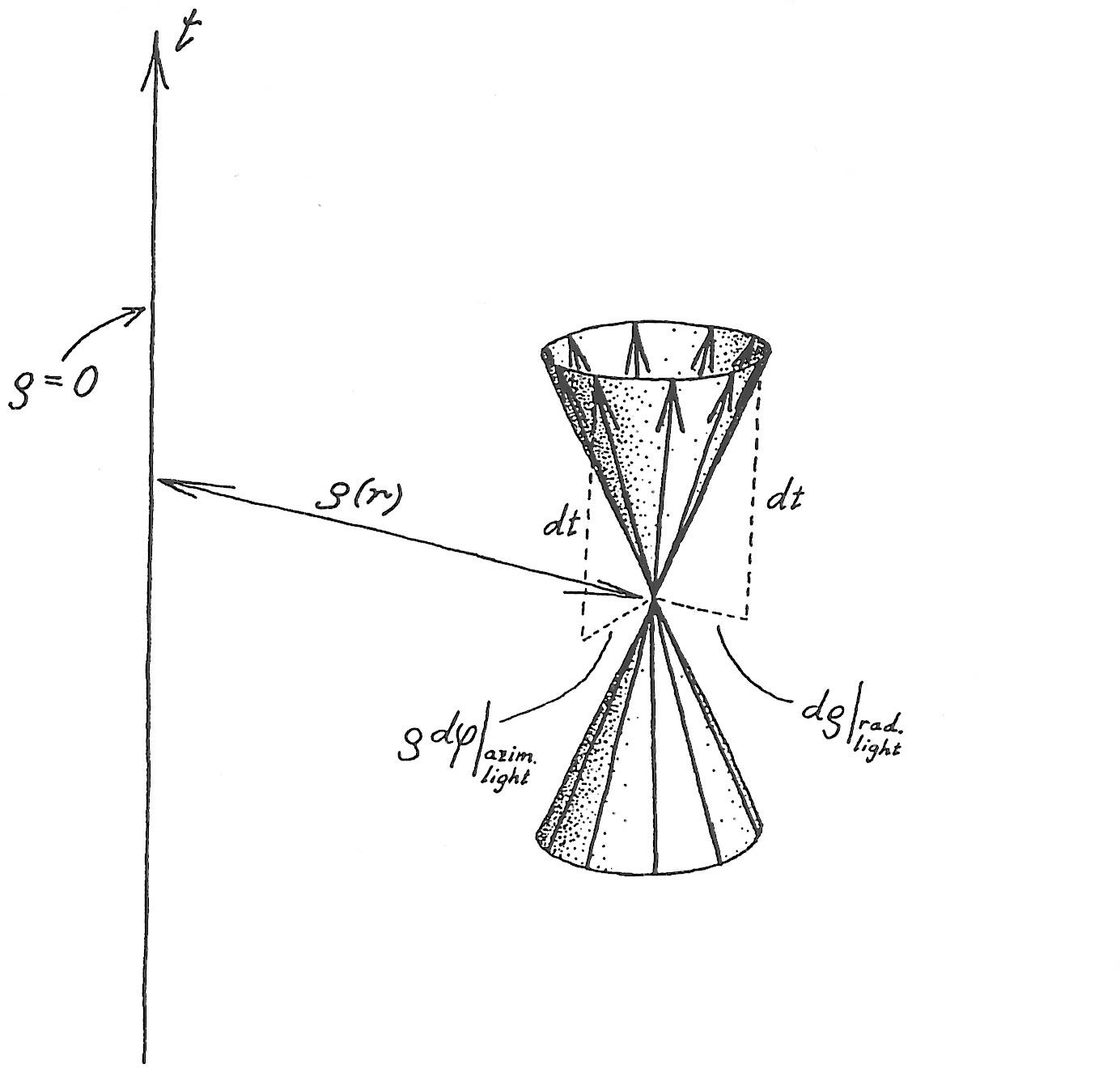
Figure 10: The advantage of sausage coordinates is that the light cone is a circular cone at every point, even if its opening angle depends on the radial coordinate $\rho$.

As a rule of thumb, all calculations are simplified by the embedding coordinates $X,Y,U,V$, while the sausage coordinates $t,x,y$ are superior for drawing pictures.

The pictures: It looks like a salami sliced by Poincaré disks, and we assume that the reader is familiar with the geodesics and the isometries in these disks. Since space is manifestly conformally flat a light cone looks like a right circular cone in the neighbourhood of any point, although its opening angle depends on the radial coordinate $\rho$ (Fig. 10). On $\mathscr{I}$ light rays slope 45 degrees. It is useful to know what a lightcone with a vertex on $\mathscr{I}$ looks like, and this is shown in Fig. 11. The flow of the Killing vector $J_{YV}$ is shown in Fig. 12. Its Killing horizon has a bifurcation line at $Y=V=0$. At $U=0$ ($t=0$) it acts as a hyperbolic translation in the Poincaré disk, and at $V=0$ ($t=\pi/2$) it acts like a Lorentz boost. This information should be kept in the back of one’s mind as one looks at the illustrations in the main text.

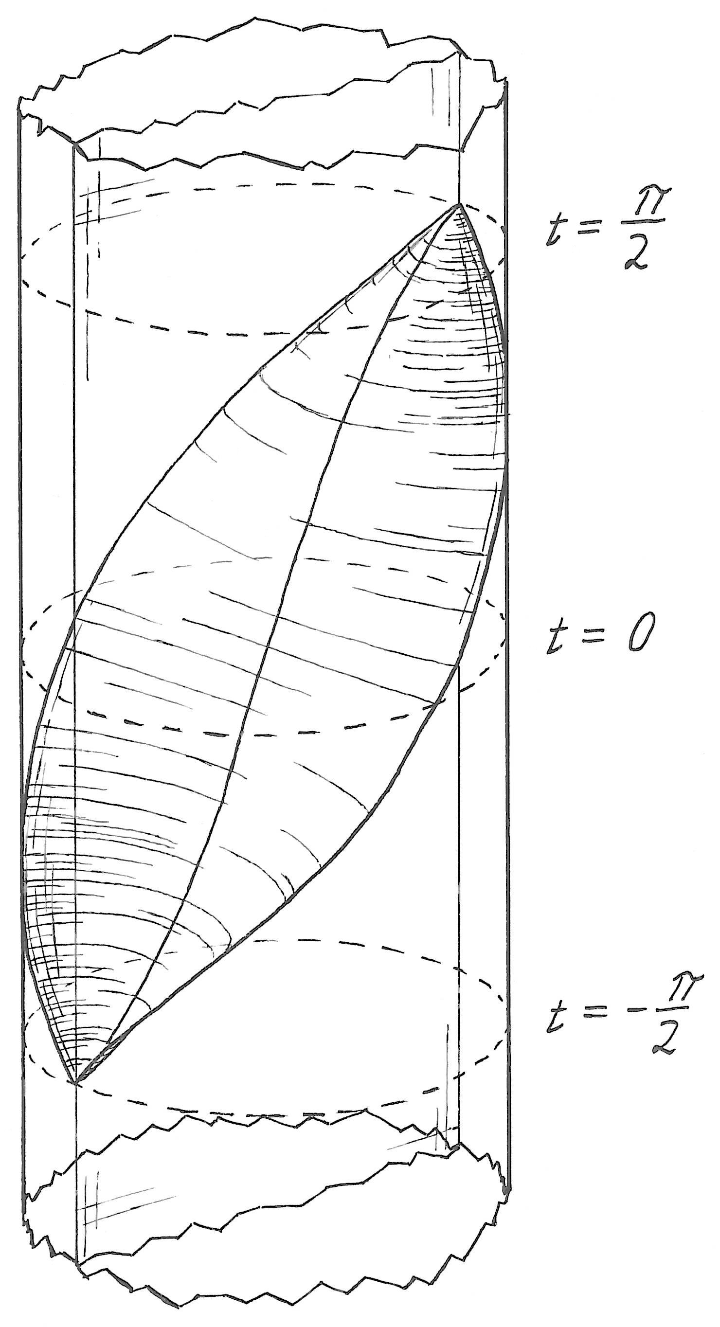
Figure 11: A light cone with its vertex on $\mathscr{I}$, or, a null plane in anti-de Sitter space. This picture is useful when thinking about the causal structure.

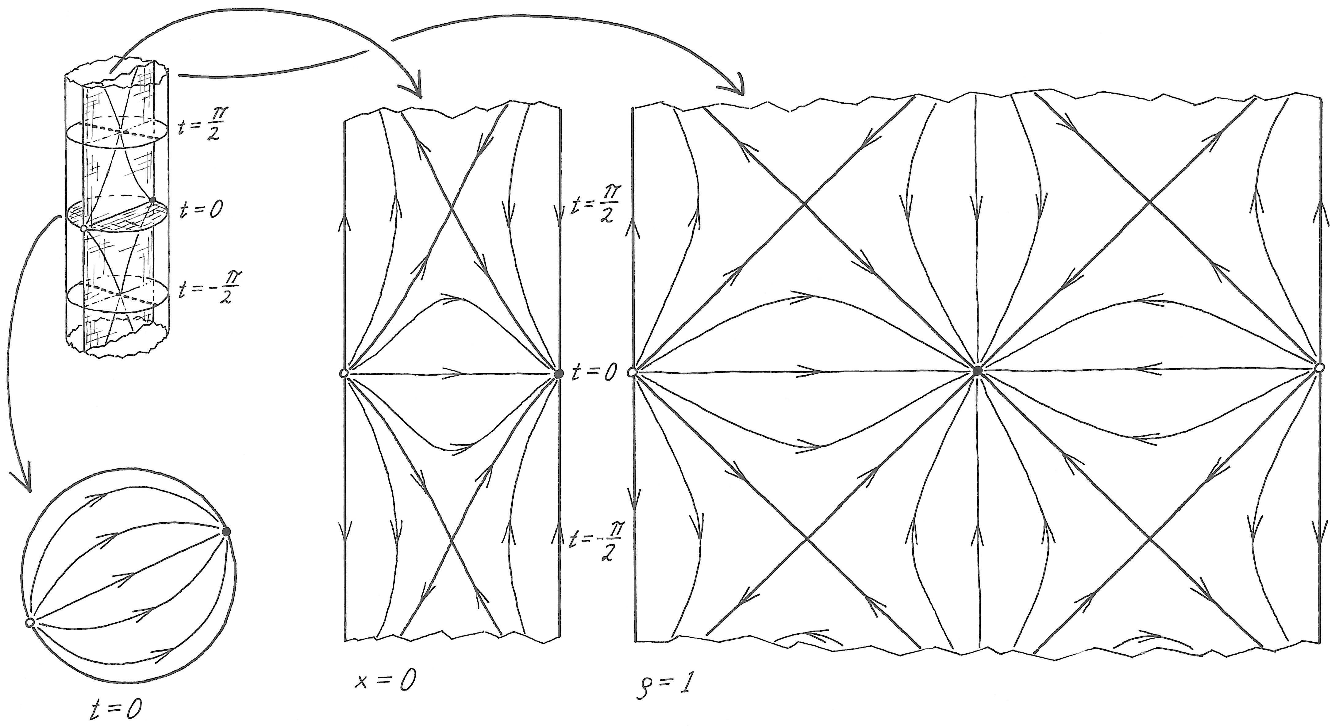
Figure 12: The flow of the Killing vector $J_{YV}$, depicted on the Poincaré disk at $t=0$, on the timelike plane $x=0$, and on the conformal boundary $\rho=1$.

Isometries: A good grasp of the isometries is useful, and easily obtained due to the curious coincidence that 2 + 1 dimensional anti-de Sitter space is identical to the group manifold of $SL(2,{\bf R})$. It can therefore be parametrized as

$$g=\left(\begin{array}[]{cc}U+Y&X+V\\ X-V&U-Y\end{array}\right)\ ,\hskip 22.76219pt\det{g}=-X^{2}-Y^{2}+U^{2}+V^{2}=1\ .$$ (34)

We placed the identity element of the group at $t=\pi/2$, well separated from the Poincaré disk at $t=0$ which in itself is a conjugacy class in the group. All isometries are of the form $g\rightarrow g_{1}gg_{2}^{-1}$, and the isometry group splits into factors according to

$$SO(2,2)=(SL(2,{\bf R})\times SL(2,{\bf R}))/Z_{2}\ .$$ (35)

The conformal boundary: The conformal boundary $\mathscr{I}$ , at $\rho=1$, is a useful platform from which to read the pictures. The group $SO(2,2)$ acts as the conformal group there. The two factors into which it splits act independently as Möbius transformations on the null coordinates $v=t+\phi$ and $u=t-\phi$. A full description can be found elsewhere [14].

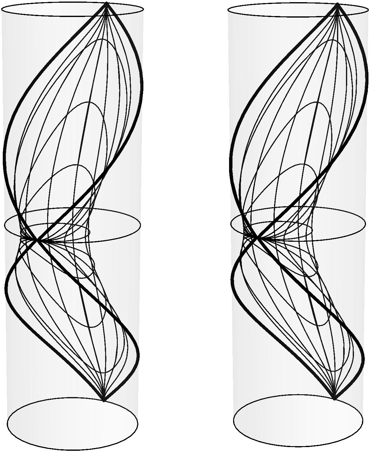
Figure 13: $1+1$ dimensional Minkowski space embedded in $2+1$ dimensional anti-de Sitter space, as a stereogram. The Poincaré disk at $t=0$ is shown.

A reference surface: Finally, to give the reader something to compare the black hole surfaces to, we give the embedding of Minkowski space into anti-de Sitter space in Fig. 13. It cuts the Poincaré disk at $t=0$ in a circle touching the boundary at a point. Such a circle is called a horocircle.

References

- [1] R. Geroch, Limits of spacetimes, Commun. Math. Phys. 13 (1969) 180.
- [2] I. Robinson and Y. Ne’eman, Seminar on the embedding problem, Rev. Mod. Phys. 37 (1965) 201.
- [3] D. Marolf, Spacetime embedding diagrams for black holes, Gen. Rel. Grav. 31 (1999) 919.
- [4] S. Deser and O. Levin, Mapping Hawking into Unruh thermal properties, Phys. Rev. D59 (1999) 064004.
- [5] M.-T. Wang and S.-T. Yau, Isometric embeddings into the Minkowski space and new quasi-local mass, Commun. Math. Phys. 288 (2009) 919.
- [6] C. Fronsdal, Completion and embedding of the Schwarzschild solution, Phys. Rev. 116 (1959) 778.
- [7] S. A. Paston and A. A. Sheykin, Global embedding of the Reissner-Nordström metric in the flat ambient space, SIGMA 10 (2014) 003.
- [8] S. M. Carroll, M. C. Johnson, and L. Randall, Extremal limits and black hole entropy, JHEP 11 (2009) 109.
- [9] H. F. Rúnarsson, Limits and special symmetries of extremal black holes, MSc Thesis, Stockholm 2012.
- [10] G. H. Brigman, Acausal geodesics in the Reissner-Nordstrøm geometry, Tensor, N. S. 25 (1972) 267.
- [11] J. T. Giblin, D. Marolf, and R. H. Garvey, Spacetime embedding diagrams for spherically symmetric black holes, Gen. Rel. Grav. 36 (2004) 83.
- [12] S. K. Chakrabarti, R. Geroch, and C.-b. Liang, Timelike curves of limited acceleration in general relativity, J. Math. Phys. 24 (1983) 597.
- [13] W. E. Couch and R. J. Torrence, Conformal invariance under spatial inversion of the extreme Reissner-Nordström black holes, Gen. Rel. Grav. 16 (1984) 789.
- [14] S. Åminneborg, I. Bengtsson, and S. Holst, A spinning anti-de Sitter wormhole, Class. Quant. Grav. 16 (1999) 363.
- [15] F. M. Paiva, M. C. Rebouças, and M. A. H. MacCallum, Limits of spacetimes—a coordinate free approach, Class. Quant. Grav. 10 (1993) 1165.