UKIRT Widefield Infrared Survey for Fe⁺

Abstract

The United Kingdom Infrared Telescope (UKIRT) Widefield Infrared Survey for Fe⁺ (UWIFE) is a 180 deg² imaging survey of the first Galactic quadrant ($7\mbox{${}^{\circ}$}<l<62\mbox{${}^{\circ}$}$; $|b|\la 1\aas@@fstack{\circ}5$) using a narrow–band filter centered on the [Fe 2] 1.644 $\mu\mathrm{m}$ emission line. The [Fe 2] 1.644 $\mu\mathrm{m}$ emission is a good tracer of dense, shock–excited gas, and the survey will probe violent environments around stars: star-forming regions, evolved stars, and supernova remnants, among others. The UWIFE survey is designed to complement the existing UKIRT Widefield Infrared Survey for $\mathrm{H}_{2}$ (UWISH2; Froebrich et al., 2011). The survey will also complement existing broad-band surveys. The observed images have a nominal 5$\sigma$ detection limit of 18.7 mag for point sources, with the median seeing of 0.83″. For extended sources, we estimate surface brightness limit of $8.1\times 10^{-20}$ W m^-2 arcsec^-2 . In this paper, we present the overview and preliminary results of this survey.

1 Introduction

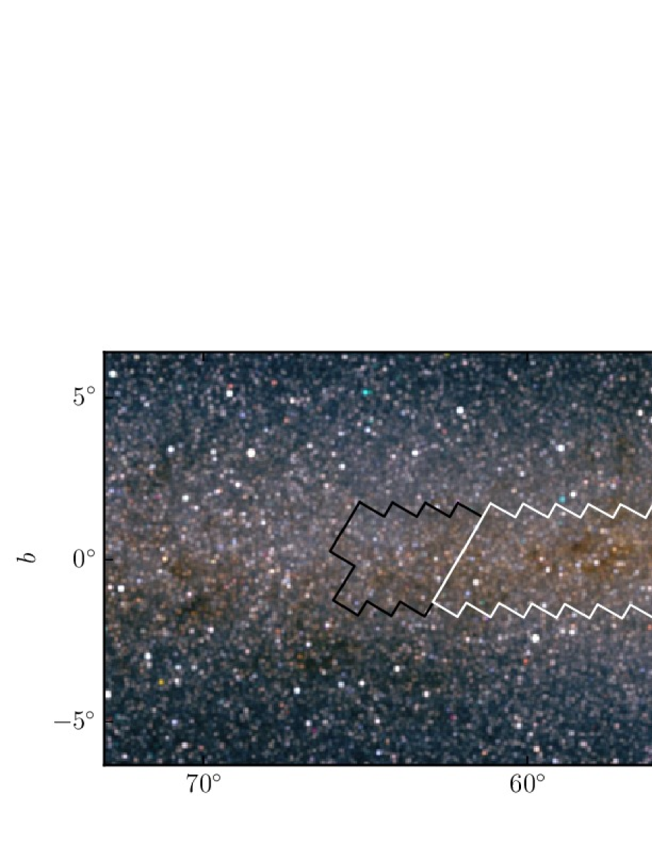
Figure 1: An overview of the UWIFE survey area in the Galactic plane, which are shown as the white polygons. The background RGB composite image are the 2MASS K, H and J bands, respectively. The black square in the lower right corner shows a nominal size and orientation of a single tile. The exact orientation of a tile will slightly change along the Galactic plane as the orientation of the equatorial axis changes. We note that the UWISH2 survey has completed its survey by 2011 and has observed a total of 234 tiles (see texts for the definition of a tile), which is slightly more than 224 tiles they originally planned (F2011). The survey coverage we adopted is based on their actual observations.

Stars, especially the massive ones, greatly influence the interstellar medium (ISM) around them. The influence is not only due to the stellar radiation but also often via dynamical interaction, e.g., jets and outflows from protostars and mass-loss from evolved stars. One of the most extreme case is their explosion as supernovae (SNe). They heat and excite the interstellar gas, and also provide turbulent motions in the ISM. ‘Mass return’ from stars to the ISM is particularly important as it contributes to metal enrichment of the universe. Study of how the stars interact with their surrounding is thus of crucial importance not only to understand the formation and evolution of stars but also to understand the evolution of galaxies.

Emission lines are great probes of processes associated with the birth and death of stars. The most popular emission lines would be hydrogen Balmer lines in the optical. The Balmer lines are often emitted by gas ionized by young hot stars, thus are used as a measure of the current star formation rate of galaxies (Kennicutt, 1998). The Balmer lines have played critical roles for studying Galactic objects, and large scale imaging surveys of the Galactic plane in H$\alpha$ line (e.g., Parker et al., 2005; Drew et al., 2005) have been a major resource for various studies. The usage of Balmer lines, however, is limited for distant or embedded objects due to relatively high extinction in the visual band.

With the advent of large–format infrared (IR) detectors, various efforts of imaging surveys of lines in near–infrared (NIR) bands have been made. The UKIRT Widefield Infrared Survey for $\mathrm{H}_{2}$ (UWISH2; Froebrich et al., 2011, F2011 hereafter) is one such survey that probes $\mathrm{H}_{2}$ 1–0 S(1) emission at 2.122 $\mu\mathrm{m}$. Using the Wide-Field Camera onboard the 3.8-m UKIRT, the survey covered the northern portion of the Galactic plane of the GLIMPSE survey (Churchwell et al., 2009). $\mathrm{H}_{2}$ emission often traces outflows and jets from embedded young stars and the regions around massive stars that are radiatively excited.

Other prominent emission lines in NIR are lines from Fe⁺. The Fe⁺ ion has four ground terms, each of which has 3 – 5 closely-spaced levels to form a 16 level system (Pradhan & Nahar, 2011). The energy gap between the ground level and the excited levels is less than $1.3\times 10^{4}$ K, making these levels easily excited in the postshock cooling region. The emission lines resulting from the transitions among them appear in optical- to far-infrared bands. In the NIR JHK bands, 10–20 [Fe II] lines are visible where the two strongest lines are at 1.257 and 1.644 $\mu\mathrm{m}$ (Koo, 2013).

The [Fe 2] lines are relatively strong in shocked gas rather than photoionized gas because Fe atoms in photoionzed gas are likely in higher ionization stages, and also because the Fe abundance in shocked gas is probably enhanced by dust destruction (Koo, 2013). Behind radiative atomic shocks, [Fe II] emissions are mostly emitted from the cooling region. For example, the ratio of [Fe 2] 1.644 $\mu\mathrm{m}$ to hydrogen Pa$\beta$ line in supernova remnants (SNRs) is between 2 and 7, while it is as low as $0.013$ in starforming regions in Orion (Oliva et al., 1989; Mouri et al., 2000). Therefore, [Fe II] forbidden lines could be used as tracers of fast radiative atomic shocks, although they can be emitted from photoionized gas when ionized by high energy photons such as X-rays, e.g., in active galactic nuclei (Mouri et al., 2000).

Here we present an unbiased survey of a portion of the Galactic Plane in [Fe 2] 1.644 $\mu\mathrm{m}$ emission, dubbed as UKIRT Widefield Infrared Survey for Fe⁺ or UWIFE. The survey was aimed to detect ionized Fe objects (IFOs), where the [Fe 2] line will highlight regions of predominantly shock-excited dense gas. [Fe 2] emission is an excellent tracer of dense outflows in young and massive star forming regions, eruptive mass loss from evolved stars, and dense media interacting with SNRs. The survey was designed to cover the same region and to complement the UWISH2 survey. The UWIFE survey was conducted with the same telescope and detector combination as in the UWISH2 survey, but only with a different filter. Further, the survey complement the UKIDSS Galactic Plane JHK survey (GPS; Lucas et al., 2008), and various other surveys like the IPHAS H$\alpha$ survey (Drew et al., 2005), the VLA 5 Ghz CORNISH survey (Hoare et al., 2012), etc.

The UWIFE survey started its initial observations in the summer of 2012 and has been completed in September of 2013. In this paper, we define the survey (§ 2) and describe its characteristics (§ 3). Our survey is briefly compared to H$\alpha$ surveys in § 4. We further outline the scientific objectives of the survey with some preliminary results when available (§ 5). § 6 concludes the paper.

Figure 2: Footprints of the UWIFE survey. The white boundary outlines the UWIFE survey area. The grey rectangles are coverage of individual tiles. The background RGB composite image are from the Spitzer GLIMPSE and MIPSGAL survey. Blue and green represents IRAC 3.6 $\mu\mathrm{m}$  and 8 $\mu\mathrm{m}$, while red is MIPS 24$\mu\mathrm{m}$. Note that there are slight gaps between adjacent tiles near $l\sim 16\mbox{${}^{\circ}$}$.

2 TARGET AREA and OBSERVATION

The UWIFE survey was conducted using the Wide-Field Camera (WFCAM, Casali et al., 2007) at UKIRT. The camera has four Rockwell Hawaii-II HgCdTe arrays. Each array has 2048 $\times$ 2048 pixels, corresponding to $13.65\arcmin\times 13.65\arcmin$ field–of–view with a pixel scale of 0.4 arcsec. They are arranged in a square pattern, with a gaps of $12.83\arcmin$ between adjacent arrays. With this layout, observing at four discrete positions results in a contiguous area covering 0.75 deg² on the sky (a WFCAM tile). For each pointing, images were obtained taken at three jitter positions. The jitter offsets were ($0\arcsec$, $0\arcsec$), ($6\aas@@fstack{\prime\prime}4$, $0\arcsec$) and ($6\aas@@fstack{\prime\prime}4$, $6\aas@@fstack{\prime\prime}4$). About each jitter position, we performed a 2 $\times$ 2 microstep with offset size of $4.62\arcsec$, to fully sample the point spread function. Three jitter positions with $2\times 2$ microstepping give total of 12 images. An exposure time of 60 seconds was used, giving a total per-pixel integration time of 720 seconds. The final stacked images are resampled to 0.2″.

The survey covered a region within the First Galactic Quadrant ($7\mbox{${}^{\circ}$}\la l\la 62\mbox{${}^{\circ}$}$; $|b|\la 1.5\mbox{${}^{\circ}$}$ ). The coverage is mostly identical to that of the UWISH2 survey except that the UWISH2 covered up to $l\simeq 65\mbox{${}^{\circ}$}$. Figure 1 shows an overview of the UWIFE survey area in the Galactic plane and compares it with the UWISH2 survey area. The survey area consists of 220 tiles, where a single tile is a square of $54\arcmin\times 54\arcmin$, aligned in equatorial coordinates. The tiles are arranged as 55 stripes of four consequent tiles along lines of constant declination (see Figure 2). The position of tiles are identical to those of UWISH2, except 20 tiles in $43\mbox{${}^{\circ}$}<l<48\mbox{${}^{\circ}$}$. For these tiles, the coordinates of UWISH2 differ from those of the GPS by a few arcminutes (they are identical otherwise), and we adopted the coordinates of the GPS. There are small gaps around $l\sim 16\mbox{${}^{\circ}$}$ not covered by the survey. The gaps inherit from the survey area of UWISH2. However, we consider the impact of the gaps on the survey as minimal.

3 Results

3.1 [Fe 2] Filter

The [Fe 2] 1.644 $\mu\mathrm{m}$ filters were not available on WFCAM, so a set of new filters were procured from JDS Uniphase Corporation and installed during the summer of 2012. The filters have a central wavelength of 1.644 $\mu\mathrm{m}$ with transmittance of 85% and effective bandwidth of 0.026 $\mu\mathrm{m}$. Figure 3 plots the filter response curve of the [Fe 2] filter provided by the manufacturer together with that of H band filter. Figure 4 shows the first light image obtained using the newly installed filter, on the SNR G11.2$-$0.3. The image is continuum-subtracted as described in section  3.3. The figure shows a comparison of our image with the [Fe 2] image of the same target obtained with the WIRC onboard the Palomar Hale telescope (Koo et al., 2007). Our UKIRT WFCAM image is basically identical to that of the WIRC, but shows more details that were not available in the WIRC image.

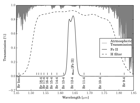
Figure 3: The response curve of the narrow-band [Fe 2] 1.644 $\mu\mathrm{m}$ filter (solid black), broad-band H (dashed black), and atmospheric transmission curves (gray line).

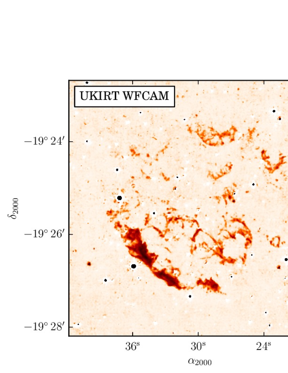
Figure 4: (left) UWIFE image of the SNR G11.2$-$0.3, which was taken with the new [Fe 2] 1.644 $\mu\mathrm{m}$ filter installed in WFCAM. (right) Image of same region taken with [Fe 2] 1.644 $\mu\mathrm{m}$ filter on WIRC in Palomar Hale telescope (Koo et al., 2007).

3.2 Survey Status & Data Quality

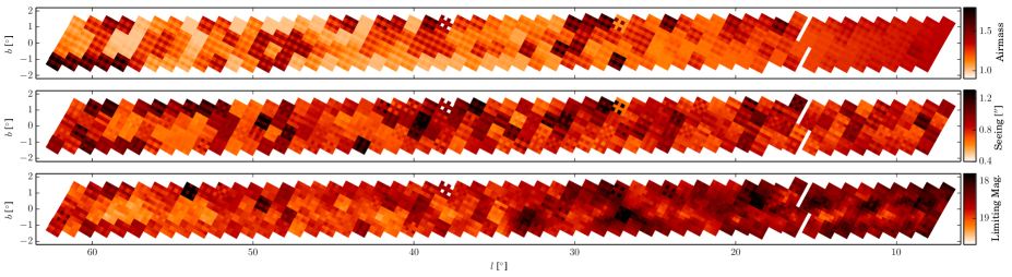
Figure 5: Distributions of airmass, seeing, and limiting magnitude of the obtained images at their sky positions.

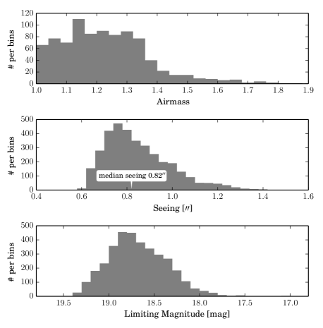
Figure 6: Histogram of the airmass, seeing and limiting magnitude.

The UWIFE observations were conducted during 2012 and 2013 and we have observed total of 220 tiles. The images were reduced by the Cambridge Astronomical Survey Unit (CASU), using the same pipeline used for reducing the images of UWISH2 and GPS. The CASU reduction steps are described in detail by Dye et al. (2006); astrometric and photometric calibrations (Hodgkin et al., 2009) are done using 2MASS catalogue.

Figure 5 displays airmass, seeing, and limiting magnitudes for 220 tiles (one tile consists of 16 images). The values are shown for each image of a single chip. For airmass values, 4 images in the same sequence share a same value, resulting in a particular pattern in the plot. The seeing values are obtained from the CASU pipeline products, and measured from the co-added frames. The statistics of these values are also shown in Figure 6 as histograms. The majority of the data have a seeing between 0.6″and 1.0″. The median seeing is 0$\aas@@fstack{\prime\prime}$82, which is slightly worse than that of UWISH2 survey (0$\aas@@fstack{\prime\prime}$73). Virtually all the images have seeing better than 1$\aas@@fstack{\prime\prime}$5.

The 5$\sigma$ limiting magnitudes are estimated following the definition of Dye et al. (2006).

$$m=m0-0.05*(X-1)-2.5\log_{10}\left(\frac{5\sigma_{sky}(1.2N)^{1/2}}{t_{\mathrm{exp}}}\right)-m_{\mathrm{ap}}$$

$m0$, $\sigma_{sky}$, and $m_{ap}$ are the zero point magnitude, sky noise and the aperture correction value, which are obtained from the FITS header of the pipeline products (Header keyword of MAGZPT, SKYNOISE and ACOR3). $X$ is the airmass and N is the number of pixels in a given aperture (aperture size of 1″ is used corresponding to the header value of APCOR3). The photometric calibration of the CASU pipeline is done with the 2MASS point source catalog and H band magnitudes are used for calibration of [Fe 2] images where the zero magnitude flux is $1.133\times 10^{-13}$ W cm^-2 $\mu\mathrm{m}$^-1 (Cohen et al., 2003). The typical values of $m0$, $\sigma_{sky}$, and $m_{ap}$ are 22.25 mag, 20 counts, and 0.2 mag, respectively. For most images, the calculated limiting magnitudes are fainter than 18 mag, with a modal value around 18.7. However, we expect the real limiting magnitudes to be brighter as crowding along the Galactic plane is not fully accounted when sky noise values are estimated. Similarly, from the $\sigma_{sky}$ values, we estimate a typical rms noise level of $8.1\times 10^{-20}$ W m^-2 arcsec^-2 for diffuse [Fe 2] emission, where we used an effective filter bandwidth of 0.026 $\mu\mathrm{m}$. Again, this would have been underestimated in the inner Galactic regions.

3.3 Continuum Subtraction

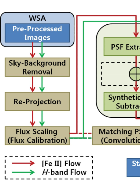
Figure 7: The Flow chart of processes adopted for the conitnuum subtraction.

The observed [Fe 2] images are continuum-subtracted using the H –band images from the GPS. The H–band images are regridded and rescaled to match the astrometry and the flux scale of the corresponding [Fe 2] images. The point–spread–function (PSF) of [Fe 2] images and corresponding H images often differ significantly. To compensate the effect of the different PSF, an image of a better seeing can be convoluted to match the poorer seeing of the other image. However, this approach is not optimal as the resulting difference image have PSF of the poorer seeing. This is an important issue for [Fe 2] emission since [Fe 2] emission is often knotty and compact. To keep the original seeing of the [Fe 2] emission, we adopted an alternative continuum subtraction method where we subtract point-like sources from the images by modeling the PSF. Below, we describe more details of this method.

1. We first re-project the H-band image to the corresponding [Fe 2] image so that the two images are astrometrically aligned.

2. We extract a $51\times 51$ pixel area around well-isolated stars whose fluxes are greater than $30\sigma$ above the background. They are normalized and median-averaged to form the PSF image. To compensate the spatial variation of PSF across the focal plane, A single chip area (4096 $\times$ 4096 pixels) is divided into sub-regions and PSFs are estimated in each sub-region, where we find $4\times 4$ sub-regions are mostly adequate.

3. We perform PSF photometry. Among the detected sources, we reject sources that are not point-like (sources with a PSF correlation coefficient less than 0.7). The source catalogues of [Fe 2] and H–band are matched and we further reject sources that have a brightness difference larger than 20% and/or a position difference larger than 0.5 pixels. With the second step we distinguish between continuum point sources and unresolved line emission features.

4. We reconstruct synthetic images using the source catalogue and the PSFs. These synthetic images are subtracted from the original images. This step is done for both [Fe 2] and H–band images, and it removes most of the point-like continuum sources from both images.

5. We then subtract the point-sources-removed H–band images from the point-sources-removed [Fe 2] images. This is to remove other extended continuum sources that escaped our detection in previous steps.

Figure 7 shows the overall flowchart of our continuum–subtraction method. We primarily used Starfinder (Diolaiti et al., 2000) for the PSF photometry together with Scamp (Bertin, 2006) and Swarp (Bertin et al., 2002) for the astrometry and the image reprojection.

We note that the difference image between [Fe 2] and H–band images may have contamination other than [Fe 2] emission. The GPS images are taken during 2005–2008, and the difference may due to source variability over more than a few years of period, in particular for point sources. It is also possible that there is some, but not significant, contributions from lines other than [Fe 2] 1.644 $\mu\mathrm{m}$, or a differing continuum slope. For example, the hydrogen Br 12 line is within the bandwidth of our [Fe 2] filter. However, we believe its contribution in the continuum-subtracted images are not significant as the H band images contain Br 10 – 18 lines and a good fraction of the Br 12 line is subtracted when H band images are subtracted.

3.4 Data Release

All the images from the survey and the continuum-subtracted images will be made public eventually through our survey web page (http://gems0.kasi.re.kr/uwife). At the time of writing, all the CASU pipeline products are available together with most of the continuum-subtracted images. The web page also provides pre-generated RGB composite images (UWISH2, UWIFE and GPS J for red, green and blue, respectively) of the entire survey region that are zoomable down to resolution of 0$\aas@@fstack{\prime\prime}$4.

4 Comparison with H$\alpha$ Surveys

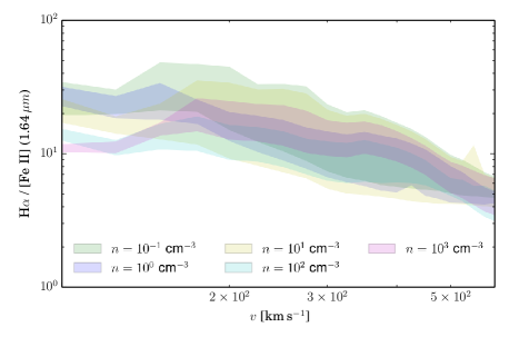
Figure 8: The ranges of model–calculated intrinsic line ratios of [Fe 2] 1.644 $\mu\mathrm{m}$ to H$\alpha$ as a function of shock velocities from the shock grids of the Solar abundances from Allen et al. (2008). Different colors represent different preshock densities. The vertical range of each plot corresponds the range of magnetic parameters ($B/n^{1/2}$) from $10^{-4}$ to $10$ $\mu$G cm^3/2.

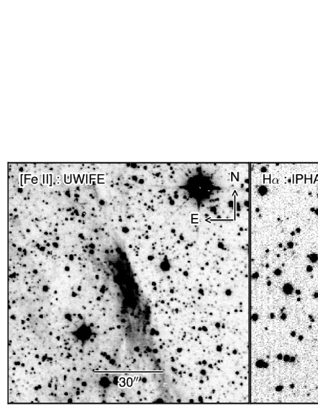
Figure 9: Northwestern part of SNR 3C391 centered at ($l$, $b$) = (31^∘ 52$\arcmin$ 08$\aas@@fstack{\prime\prime}$7, +2^∘ 07$\arcmin$ 28$\aas@@fstack{\prime\prime}$5). It shows bright [Fe 2] emission in UWIFE survey while H$\alpha$ emission from IPHAS survey is not detected. Total hydrogen column densities toward 3C391 is estimated as $2\times 10^{22}$ cm⁻², corresponding to a visual extinction A_V $\sim$ 10 mag (Rho & Petre, 1996).

The [Fe 2] forbidden lines, in particular the line at 1.644 $\mu\mathrm{m}$, are good tracers of fast radiative atomic shocks. The intrinsic emissivity of [Fe 2] line at 1.644 $\mu\mathrm{m}$ from atomic shocks could be fainter than other tracers in optical bands (e.g., H$\alpha$) in general. However, this can easily be compensated by lower extinction in the infrared for embedded objects, or those at large distances from us.

Figure 8 shows model–calculated intrinsic line ratios of H$\alpha$ to [Fe 2] 1.644 $\mu\mathrm{m}$ for various shock conditions assuming solar abundances adopted from the shock grids of Allen et al. (2008). The models suggest that the H$\alpha$ emission is intrinsically brighter than the [Fe 2] emission by an order of magnitude for interstellar shocks of given shock velocity range of 100 to 500 $\mathrm{km\,s}^{-1}$. The ratio can become as high as $\sim 50$ for slower shocks and as low as $\sim 5$ for faster shocks.

The line ratios given above do not take the interstellar extinction into account. Due to relatively lower extinction in the infrared, when compared to that in the optical, the [Fe 2] lines can appear brighter than H$\alpha$ for objects with high foreground absorption. We may define the amount of differential extinction between [Fe 2] and H$\alpha$ for a given Av as $10^{-2.5\times(\mathrm{A}(1.644\mu m)-\mathrm{A}(0.656\mu m))}$. For example, we get $\sim 30$ for Av of 6 mag. This means that, although [Fe 2] is intrinsically fainter by a factor of $30$, [Fe 2] look as bright as H$\alpha$ for Av of 6 mag. According to Figure 8, the intrinsic line ratios of H$\alpha$ to [Fe 2] 1.644 $\mu\mathrm{m}$ range from $5$ to $50$, and it is expected that [Fe 2] becomes apparently brighter than H$\alpha$ for objects with Av higher than several magnitudes. The visual extinction of 6 mag is expected for nominal hydrogen column density of $N_{\mathrm{H}}=10^{22}$ cm^-2, thus [Fe 2] 1.644 $\mu\mathrm{m}$ line would be often brighter than H$\alpha$, particularly for objects in the inner galaxy.

The above comparison does not take account the sensitivity of the underlying detector system. Because of the high sky background in the NIR when compared to that in the optical, a better sensitivity is usually obtained at optical wavelengths, although it depends on various other factors such as the telescope diameter. One of the surveys that well complements our [Fe 2] survey is the INT/WFC Photometric H$\alpha$ Survey of the Northern Galactic Plane (IPHAS), which is an H$\alpha$ imaging survey being carried out using the 2.5m Isaac Newton Telescope. The IPHAS survey has an H$\alpha$ surface brightness limit of $10^{-20}$ W m^-2 arcsec² (Sabin et al., 2013), which is comparable to the surface brightness limit of our survey. Therefore, the UWIFE survey will have advantage over IPHAS survey for sources with Av greater than several magnitudes. Figure 9 shows one example at A_V $\sim$ 10 mag where we see bright [Fe 2] emission while H$\alpha$ emission is absent.

5 Discussion

5.1 Jets/Outflows from Young Stars

Outflows are ubiquitous in low- to high-mass star formation (Shepherd & Churchwell, 1996), so they are significant signposts in searching for star forming regions. Since the discovery of Herbig-Haro (HH) objects (Herbig, 1950; Haro, 1952) in the optical, many different types of outflows have been reported over a wide range of wavelengths, from X-ray to radio (Lada, 1985; Bachiller, 1996; Reipurth & Bally, 2001; Shepherd, 2005; Bally et al., 2007). Each emission line in the various wavelength realms from X-ray to the radio shows different aspects in the physical and chemical conditions in the shocks. In the near-infrared, [Fe 2] and H₂ emission lines are good tracers for outflows and jets and have often been observed in low-mass star forming regions (Davis & Eisloeffel, 1995; Reipurth et al., 2000; Davis et al., 2003; Hayashi & Pyo, 2009). Generally [Fe 2] emission traces partially ionized, fast, and dissociative J-shocks, while $\mathrm{H}_{2}$ emission traces neutral, slow, C-shocks or non-dissociative shocks (Hollenbach & McKee, 1989a; Smith, 1994). These two emission lines show different spatial distribution and properties each other as demonstrated in Figure 10. While the [Fe 2] emission is confined in narrow jets or relatively compact knots at the tip of jets, $\mathrm{H}_{2}$ emission can be more extended. The fast well collimated [Fe 2] jets close to the driving sources provide the clue of the launching machanism (Pyo et al., 2003, 2006, 2009).

In the UWIFE survey region, there are thousands of small star forming regions (Avedisova, 2002). There are many objects related to the outflow phenomenon detected at various wavelength: 202 MHOs (Molecular hydrogen emission-line Objects: Davis et al., 2010), 106 EGOs (Extended Green Objects in GLIMPSE survey: Cyganowski et al., 2008), 55 CO outflows (Wu et al., 2004a), 239 6.7-Ghz methanol masers (Pestalozzi et al., 2005), 57 Class I Methanol masers (Val’tts & Larionov, 2007), 170 OH masers (Szymczak & Gérard, 2004). On the other hand, number of HH obejcts and alike are relatively small in this region. Most of HH objects are concentrated in the region of 100^∘$<$ $l$ $<$ 220^∘, and only several sources are reported in our survey region: 7 HH objects (Herbig-Haro Objects: Reipurth, 2000) and 4 HBC sources (Herbig-Bell Catalog: Herbig & Bell, 1988). UWIFE-SYSOP (UWIFE-Searching for the Young Stellar Outflows Project) is a project to find IFOs associated with YSOs. In this project, we will not only make the general catalog of the IFOs but also study the statistics of outflows and their physical quantities with the evolutionary stages of YSOs.

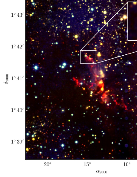
Figure 10: RGB colour composite image of the star-forming region G35.2N. Red, green and blue each represents narrow band $\mathrm{H}_{2}$ from the UWISH2, narrow band [Fe 2] from the UWIFE and broad–band J from the GPS. Unlike broadly distributed $\mathrm{H}_{2}$ emission, [Fe 2] is shown as compact emission at the tip of jets.

5.2 Massive Star Forming Regions

The formation of massive stars ($M\ga 8\,M_{\sun}$) is still unclear in many aspects (Zinnecker & Yorke, 2007). One question to be cleared is how massive stars obtain their mass. It has been increasingly reported that, as in low-mass stars, the disk-mediated accretion process seems to be underway in forming massive stars (e.g. Beuther et al., 2002; Wu et al., 2004b; San José-García et al., 2013; Cooper et al., 2013). However, it is still uncertain if such a disk accretion works in the mass range of $M\ga 25\,M_{\sun}$ (Zinnecker & Yorke, 2007). One way to grasp the accretion process is tracing the outflow features, because the outflow process is closely related with the disk accretion process (cf. section 5.1). In the following sections, we describe how UWIFE will contribute to the elucidation of massive star formation through the jet and outflow phenomena.

5.2.1 Outflow Features in Infrared Dark Clouds

Infrared dark clouds (IRDCs), seen silhouette against the bright Galactic background in mid-infrared (MIR), are cold ($<25$ K) and very dense ($n_{\rm H_{2}}>10^{5}{\rm cm}^{-3}$) interstellar clouds with high column densities ($\sim 10^{23}-10^{25}{\rm cm}^{-2}$; Simon et al. (2006a, and references therein)) so that IRDCs are believed to be a probable sites where massive stars are forming. Due to large extinction, IRDCs have usually been studied at longer wavelengths (e.g., far-infrared or millimeter) to investigate prestellar or starless cores in IRDCs and their filamentary structures (e.g., Rathborne et al., 2006; Jackson et al., 2010; Wilcock et al., 2012). Although most IRDCs or their cores ($>50\%$) do not show a signature of on-going star formation in MIR, there are some cores with bright MIR stellar sources indicating star formation activity (Chambers et al., 2009). These star-forming cores are, however, still deeply embedded in a cloud with large extinction, and few studies are made toward IRDCs for searching for outflow features in NIR. Therefore, it is worthwhile to examine the data from an unbiased [Fe 2] survey data to detect outflows in IRDCs, particularly in rather evolved IRDCs which show active star formation for understanding the process of high-mass star formation in an early evolutionary phase.

One such cloud is the IRDC located at $(l,b)\sim(53.2,\,0.0)$ which shows a number of bright MIR stellar sources, likely YSOs, along its long, filamentary structure; here, we refer to it as “IRDC G53.2.”. The UWISH2 survey data reveals ubiquitous outflow features around YSO candidates in the IRDC G53.2 (Figure 11, left). As noted in other recent studies (e.g., Davis et al., 2009), the $\mathrm{H}_{2}$ outflows are particularly identified around earlier classes of YSOs (e.g., Class I and Flat Class) which contribute $\sim 50\%$ of the YSO candidates in the IRDC G53.2 based on the analysis of Spitzer data (Kim et al. in prep.). In the UWIFE image of the IRDC G53.2, only a few [Fe 2] emissions have been detected so far. The inset in Figure 11 (left) shows [Fe 2] emission identified around a YSO candidate in the IRDC. A point-like knot shows $\mathrm{H}_{2}$ emission as well but with a little shifted peak between the [Fe 2] and $\mathrm{H}_{2}$ emissions. A preliminary analysis suggests that the number of identified [Fe 2] emissions is much smaller compared to that of $\mathrm{H}_{2}$ emissions in the same area.

Investigation of the characteristics of [Fe 2] emissions associated with YSOs in IRDCs in the entire UWIFE survey area, where $\sim$ 300 IRDCs which have GRS counterparts (Simon et al., 2006b) are included, will provide much insight on the nature of jets and outflows of YSOs. In particular, comparative studies between the IRDCs and the low-mass star forming regions will be of importance. We note that there already are on-going or planned UWISH2 projects to search for outflows/jets toward massive star forming regions or filamentary clouds in $\mathrm{H}_{2}$ (Froebrich et al., 2011; Ioannidis & Froebrich, 2012; Lee et al., 2012). The UWIFE survey, therefore, will be a good complimentary data to expand our understanding to the physical structure of the outflows of high-mass protostars.

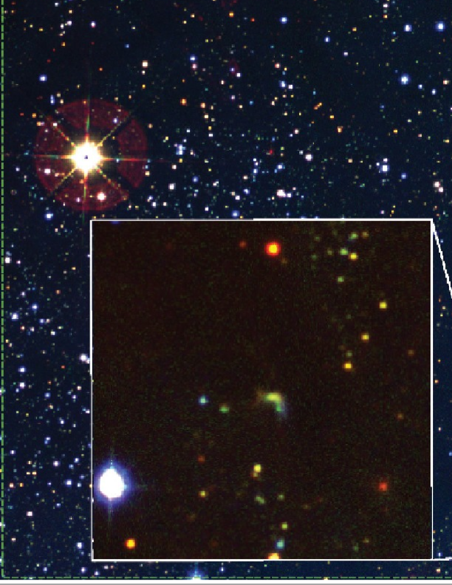
Figure 11: (Left) Three-color composite image of the center of the IRDC G53.2 made by UKIRT/WFCAM $\mathrm{H}_{2}$(R)+[Fe II](G)+J(B) from UWISH2+UWIFE+GPS. The presented region in the whole IRDC is marked by green-dashed box in the right figure. The inset presents [Fe II] emission identified in this area. (Right) Three-color composite image of the whole IRDC G53.2 made by Spitzer IRAC/MIPS 24 $\mu\mathrm{m}$(R)+8.0 $\mu\mathrm{m}$(G)+5.8 $\mu\mathrm{m}$(B). GRS ¹³CO $J=$1–0 contours are overlaid in magenta. The outermost contour presents the boundary of the IRDC.

5.2.2 Outflow Features around Ultracompact H 2 regions

An ultracompact H 2 region (UCHII) indicates a very compact H 2 region, whose typical size, density, and emission measures are $\la 10^{17}$ cm, $\ga 10^{4}$ cm^-3, and $10^{7}$ pc cm^-6, respectively (Churchwell, 2002). It is thought to be a “late” stage of massive young stellar objects (MYSOs), no longer accreting significant mass (Churchwell, 2002; Zinnecker & Yorke, 2007). More specifically, it is the period between the rapid accretion phase when the central object is being formed and the ionized phase when the larger, more diffuse, less obscured H 2 region is being produced. UCHII’s unique position in the MYSO evolutionary track enables us to study the history of accretion processes as follows.

Since UCHII’s natal clumps are not completely destroyed yet, one may expect that the materials ejected during the prior, active accretion phase produce shocked outflow features around UCHIIs. By tracing these “footprint” outflow features around UCHIIs, we can study the history of accretion process, because the outflow process is closely related with the accretion process (cf. section 5.1). These features can be observed through radiative cooling lines, such as [Fe 2] 1.64 $\mu\mathrm{m}$, H₂ 2.12 $\mu\mathrm{m}$, and CO radio lines (Hollenbach & McKee, 1989b; Neufeld & Dalgarno, 1989; Kaufman & Neufeld, 1996; Wilgenbus et al., 2000; Flower & Pineau Des Forêts, 2010). Indeed, CO outflow features have been observed around UCHII regions, such as G5.89-0.39 (Watson et al., 2007; Wood & Churchwell, 1989) and G18.67+0.03 (Cyganowski et al., 2012). The dynamical timescale of these CO outflow features is $>10^{3}$ yr, which is comparable or greater than the typical lifetime of UCHIIs ($\ga 5\times 10^{4}$ yr, Wood & Churchwell, 1989; González-Avilés et al., 2005) and MYSO jet-phase ($\sim 4\times 10^{4}$ yr, Guzmán et al., 2012).

A search for [Fe 2] features around UCHIIs are under way using a UCHII catalog. The catalog is from the CORNISH survey (Hoare et al., 2012; Purcell et al., 2013), which covers the same part of the Galactic plane as UWIFE. Shinn et al. (in prep.) have found [Fe 2] outflow features around several UCHIIs. One example, G025.3824$-$00.1812 and G025.3809$-$00.1815, is shown in Fig. 12, where the southwestward [Fe 2] outflow/jet feature is evident. The outflow feature seems to emerge from the direction towards the two UCHIIs and has a well-collimated appearance. The [Fe 2] features around UCHIIs detected from the unbiased UWIFE survey enable us to extract some general properties of the MYSO accretion process. The outflow morphology, the outflow mass loss rate, and their relation with the MYSO physical parameters would be the initial outcomes (cf. Shinn et al., 2013). Based on those results, we may investigate if the outflow features support the disk accretion process, and may infer the final stellar mass where the disk accretion seems to work.

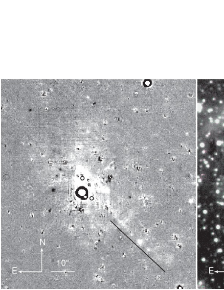
Figure 12: [Fe 2] outflow feature around a UCHII region G025.3824$-$00.1812 (upper-circle) and G025.3809$-$00.1815 (lower-circle) of Purcell et al. (2013): (left) Continuum-subtracted [Fe 2] image and (right) RGB color-composite image (R=H, G=[Fe 2], B=H). The black line indicates the outflow features.

5.3 Nebulae around Evolved Stars

Circumetellar nebulae around evolved stars are fossil record of their mass-loss history. They often represent dense structure resulting from sudden changes in wind characteristics. These circumstellar nebulae are often known from their optical emission lines, but infrared emission from cold and dense medium is becoming more important. In principle, emission in different regimes provide us with a more complete view of the progenitor star system and its evolution.

5.3.1 Planetary Nebulae

Planetary nebulae (PNe) are the most frequent type of nebula around evolved stars. The nebula consists of material ejected during the AGB phase and ionized by the UV radiation from the newly-formed hot central star (Frew & Parker, 2010). More than a thousand PNe are currently known in our Galaxy (e.g., Acker et al., 1992). However, most of the known ones are high above the Galactic plane and the number of PNe along the Galactic plane is relatively small. With the advent of sensitive H$\alpha$ survey of the Galactic plane such as IPHAS (Drew et al., 2005) and VPHAS+, a large number of PNe in the plane is being revealed (Viironen et al., 2009b, a; Sabin et al., 2010). Furthermore, the NIR line surveys like UWISH2 and UWIFE have the potential to uncover a significant population PNe along the Galactic plane. These surveys will help us to constrain their space density and any variation along the plane which is related to various routes of PN formation. Also the findings of numerous new PNe will enable more rigorous statistical analysis.

PNe are often bright in the $\mathrm{H}_{2}$ 2.122 $\mu\mathrm{m}$ line. Kastner et al. (1996) detected $\mathrm{H}_{2}$ emission from 23 PNe out of 60 PNe in their narrow-band imaging survey of 2.122 $\mu\mathrm{m}$ emission. The 2.122 $\mu\mathrm{m}$ $\mathrm{H}_{2}$ emission is most prominent in PNe of bipolar morphology and they suggested a physical connection. On the other hand, surveys of PNe in [Fe 2] 1.644 $\mu\mathrm{m}$ have been sparse. Hora et al. (1999) observed a sample of PNe with medium-resolution (R$\sim$700) near-infrared ($\lambda=1-2.5\mu\mathrm{m}$) spectra. Among 41 they observed, 16 showed $\mathrm{H}_{2}$ 2.122 $\mu\mathrm{m}$ emission but only 3 showed [Fe 2] 1.644 $\mu\mathrm{m}$ emission. While the fraction of PNe with detected [Fe 2] 1.644 $\mu\mathrm{m}$ emission was small, the emission has been useful in studying the nature of mass loss, as demonstrated in the case of M2-9 (Smith et al., 2005).

The initial search of [Fe 2] emission from the known PNe in the UWIFE survey resulted in a half dozen of detection from around 29 known PNe (25 from Acker et al. (1992) and 4 from F2011). Most of these PNe with [Fe 2] emission have accompanying $\mathrm{H}_{2}$ emission. Nonetheless, 3 of them are not detected in $\mathrm{H}_{2}$ (e.g., PN M 1-51 as in Figure 13). For comparison, Kastner et al. (1996) found all the 3 PNe detected in [Fe 2] show accompanying $\mathrm{H}_{2}$ emission. Study of PNe connecting their emission characteristics to their morphology will be important as it may reveal how the mass–loss history of progenitors affects the shaping of PNe.

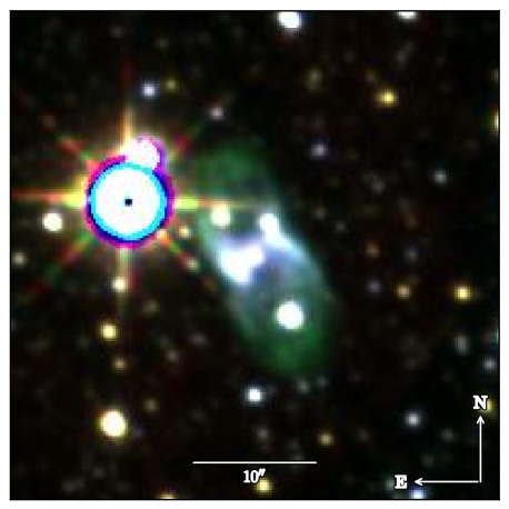
Figure 13: RGB composite image of PN M 1-51. The color scheme is same as in Figure 10. This is one of the PN showing [Fe 2] emission without $\mathrm{H}_{2}$.

5.3.2 Nebulae around Evolved Massive Stars

Mass loss in massive stars plays a more critical role than in less massive ones. An important class of evolved massive stars are luminous blue variables (LBVs). LBVs belong to the most luminous stars in our Galaxy (thus with very large initial masses) typified by their irregular variabilities, which are sometimes associated with eruptive mass loss. The best example of LBV star is $\eta$ Car which is surrounded by an extremely massive circumstellar shell ($M\sim 15⁢\mathrm{M}_{\odot}$), believed to be a product of its 1840’s great ejection. The line emission from circumstellar shells around some LBVs has been a valuable tool to understand not only the physical process responsible for LBV mass loss but also the nature of the central star. NIR lines, such as [Fe 2], are well suited to study the shells around evolved massive stars as they are less affected by interstellar extinction. [Fe 2] emission is so far found in a half dozen of LBVs (Smith, 2002), and detailed studies of $\eta$ Car have demonstrated the usefulness of the [Fe 2] emission (Smith, 2006).

In our preliminary study, we searched for [Fe 2] emission associated with known LBVs and candidate LBVs from Clark et al. (2005). Among several sources covered by the UWIFE survey, we detected [Fe 2] emission from a few of them. An example is HD 168625 as shown in Fig. 14. HD 168625 is an intriguing system showing a bipolar nebula several times larger than its equatorial dust torus (Smith, 2007), quite similar to what is found around SN 1987A. We found both $\mathrm{H}_{2}$ and [Fe 2] emission around the equatorial torus, but with different morphology. The morphology of $\mathrm{H}_{2}$ emission is similar to H$\alpha$ and the thermal emission from the dust (Pasquali et al., 2002) and is sharply peaked along the torus in the southwestern side. On the other hand, the [Fe 2] emission is more diffuse and more extended toward the northeastern side. The only other LBV that shows both $\mathrm{H}_{2}$ and [Fe 2] emission is $\eta$ Car. Follow–up spectroscopic observations of HD 168625 will reveal detailed mass–loss history of the central star, as in the case of $\eta$ Car (Smith, 2006).

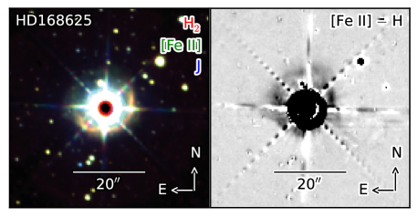
Figure 14: (left) RGB colour composite image of LBV HD168625. Red, green and blue each represents $\mathrm{H}_{2}$ from the UWISH2, [Fe 2] from the UWIFE and broad–band J from the GPS survey. (right) Continuum–subtracted [Fe 2] image of HD168625.

5.4 Supernova remnants

When a SN explodes, a strong shock with a typical expansion velocity of $\sim$ 10,000 $\mathrm{km\,s}^{-1}$ is produced, which later decelerates and becomes radiative at the speed of a few hundreds $\mathrm{km\,s}^{-1}$. Along with this front shock expanding into the surrounding medium, there exists a reverse shock which propagates back into SN material. Strong NIR [Fe 2] lines are emitted when these shocks interact with dense material, which could be either the SN or the circumstellar material for young SNRs, and usually interstellar material for middle-aged SNRs (e.g., Oliva et al., 1989, 1990; Koo et al., 2007; Lee et al., 2009; Moon et al., 2009; Lee et al., 2013, see also Koo 2013 and references therein). Moreover, Fe, being the end product of the stellar nucleosynthesis process, forms a main component of the supernova ejecta; the materials ejected from the deep layers of the progenitor are often enriched in Fe. The Fe abundance can also be significantly enhanced in a shocked region if the interstellar dust is destroyed.

In the survey area, there are over 70 known SNRs mostly identified by radio and X-ray observations (Green, 2009). We search for the [Fe 2] emission around the positions of the known SNRs. Our preliminary results reveal that 20–30 % of known SNRs show [Fe 2] emission, including previously observed [Fe 2]-emitting SNRs such as G11.2$-$0.3 (Koo et al., 2007), W 28 (Reach et al., 2005), G21.5$-$0.9 (Zajczyk et al., 2012), 3C 391 (Reach et al., 2002), 3C 396 (Lee et al., 2009), W 44 (Reach et al., 2005), and W 49B (Keohane et al., 2007). In most cases, our [Fe 2] images provide high-quality, wide-area views of detected SNRs, for which, sometimes, only parts of the area were covered by the previous observations. In addition, we find new [Fe 2]-emitting SNRs. Many of them show near-infrared H₂ emission identified by UWISH2 survey and/or thermal X-ray emission in the center, implying that they are located within dense environments. For example, Figure 15 shows a color image of 3C 391, which is one of the bright [Fe 2]-emitting SNRs in the survey area.

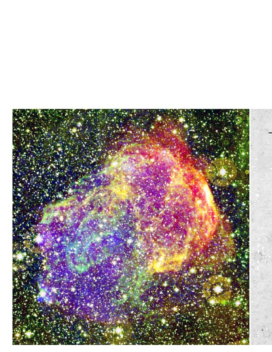
Figure 15: $Left$: Color composite figure of 3C 391, composed of 1.4 GHz radio continuum (red), H₂ 2.122 $\mu$m (yellow), [Fe 2] 1.644 $\mu$m (green), and Chandra X-ray (blue) images (Helfand et al., 2006; Froebrich et al., 2011; Chen et al., 2004). $Right$: Continuum-subtracted [Fe 2] image. Superimposed are VLA 1.4 GHz radio contours with intensity levels of 2.0, 5.6, 17, 35, and 60 mJy beam^-1 and the beam size of $6\aas@@fstack{\prime\prime}2$ $\times$ $5\aas@@fstack{\prime\prime}4$.

5.5 Other Sources and Unbiased Search

The UWIFE survey is an unbiased survey, so that we have an opportunity to detect “every” dense, shocked gas with bright [Fe 2] line emission in the inner Galaxy, some of which would be serendipitous discoveries. In order to identify IFOs in the UWIFE survey area, we search for IFOs in the continuum-subtracted [Fe 2]-line images visually using the naked eye. At the time of writing, we have detected 111 IFOs in 10.5 deg² from l=53^∘ to 60^∘. The detected sources include YSO/YSO candidates, AGB/RCB (R Coronae Borealis stars) stars and their candidates, EGOs (Extended Green Objects), and star forming regions. But most ($\sim 85$%) of them do not have counterparts in SIMBAD. The detected IFOs are classified into point-like or diffuse based on their morphology. The diffuse sources can be further divided into amorphous, cometary, jet/filamentary, or shell–like. Figure 16 shows examples of each category. To better systematize the unbiased search of IFOs, an automatic computer–aided method is being developed. We note, however, that a significant number of point-like sources we detected above might be variables instead of [Fe II]-line emitting sources.

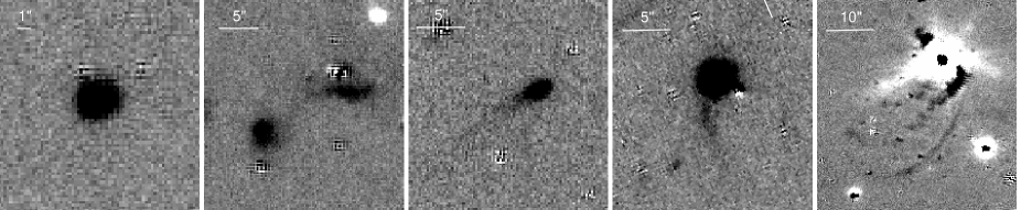
Figure 16: Continuum–subtracted [Fe 2] images of IFOs of various morphologies in the UWIFE survey area (from left to right): point-like, amorphous, cometary, jet/ filamentary and shell-like.

6 Concluding Remarks

In this paper, we present an overview and initial outlook of the UKIRT Widefield Infrared Survey for [Fe 2] (UWIFE). The UWIFE survey is an imaging survey of the first Galactic quadrant ($7\mbox{${}^{\circ}$}<l<62\mbox{${}^{\circ}$}$; $|b|\la 1\aas@@fstack{\circ}5$) using a narrow–band filter centered on the [Fe 2] 1.644 $\mu\mathrm{m}$ emission line, which is a good tracer of dense shock-excited gas. The survey started in the summer of 2012 and was completed as of 2013. The resulting images have a median seeing of 0.8″ with a 5$\sigma$ limiting magnitude of $\sim$ 19^th mag and will provide valuable resources to study the Galactic plane.

Our own Galaxy and its inner workings such as how new stars are born and die are still mysterious. Unbiased imaging surveys of the galactic plane in the infrared broadband such as Glimpse and MIPSGAL have greatly increased our understanding of the Galaxy. A significant advantage of our UWIFE survey is its complementarity with these existing and/or upcoming surveys, in particular with the UWISH2 survey. The line emission such as the [Fe 2] 1.644 $\mu\mathrm{m}$ line and the molecular hydrogen 1-0 S(1) emission line at 2.122 $\mu\mathrm{m}$ will complement the broadband surveys and probe dynamically active components of interstellar medium. The high-spatial resolution narrow-band WFCAM images from the UWIFE and UWISH2 surveys will pin–point regions of active interaction in the complex environments. Furthermore, these imaging survey will provide wealth of potential targets for follow–up spectroscopic observations.

This work was supported by K-GMT Science Program funded through Korea GMT Project operated by Korea Astronomy and Space Science Institute (KASI). H.-G. Lee acknowledges support from a Grant-in-Aid for Japan Society of Promotion of Science (JSPS) fellows (No. 23$\cdot$01322). H.-J. Kim was supported by NRF(National Research Foundation of Korea) Grant funded by the Korean Government (NRF-2012-Fostering Core Leaders of the Future Basic Science Program). D. Moon was supported by Korean Federation of Science and Technology Societies (KOFST). M.-G. Lee, B.-C. Koo, H.-M. Lee and M. Ishiguro were supported by the National Research Foundation of Korea (NRF) grant funded by the Korea Government (MSIP) (No. 2012R1A4A1028713).

References

- Acker et al. (1992) Acker, A., Marcout, J., Ochsenbein, F., Stenholm, B., Tylenda, R., & Schohn, C. 1992, The Strasbourg-ESO Catalogue of Galactic Planetary Nebulae. Parts I, II.
- Allen et al. (2008) Allen, M. G., Groves, B. A., Dopita, M. A., Sutherland, R. S., & Kewley, L. J. 2008, ApJS, 178, 20
- Avedisova (2002) Avedisova, V. S. 2002, Astronomy Reports, 46, 193
- Bachiller (1996) Bachiller, R. 1996, ARA&A, 34, 111
- Bally et al. (2007) Bally, J., Reipurth, B., & Davis, C. J. 2007, Protostars and Planets V, 215
- Bertin (2006) Bertin, E. 2006, in Astronomical Society of the Pacific Conference Series, Vol. 351, Astronomical Data Analysis Software and Systems XV, ed. C. Gabriel, C. Arviset, D. Ponz, & S. Enrique, 112
- Bertin et al. (2002) Bertin, E., Mellier, Y., Radovich, M., Missonnier, G., Didelon, P., & Morin, B. 2002, in Astronomical Society of the Pacific Conference Series, Vol. 281, Astronomical Data Analysis Software and Systems XI, ed. D. A. Bohlender, D. Durand, & T. H. Handley, 228
- Beuther et al. (2002) Beuther, H., Schilke, P., Sridharan, T. K., Menten, K. M., Walmsley, C. M., & Wyrowski, F. 2002, A&A, 383, 892
- Casali et al. (2007) Casali, M., et al. 2007, A&A, 467, 777
- Chambers et al. (2009) Chambers, E. T., Jackson, J. M., Rathborne, J. M., & Simon, R. 2009, ApJS, 181, 360
- Chen et al. (2004) Chen, Y., Su, Y., Slane, P. O., & Wang, Q. D. 2004, ApJ, 616, 885
- Churchwell (2002) Churchwell, E. 2002, ARA&A, 40, 27
- Churchwell et al. (2009) Churchwell, E., et al. 2009, PASP, 121, 213
- Clark et al. (2005) Clark, J. S., Larionov, V. M., & Arkharov, A. 2005, A&A, 435, 239
- Cohen et al. (2003) Cohen, M., Wheaton, W. A., & Megeath, S. T. 2003, AJ, 126, 1090
- Cooper et al. (2013) Cooper, H. D. B., et al. 2013, MNRAS, 430, 1125
- Cyganowski et al. (2012) Cyganowski, C. J., Brogan, C. L., Hunter, T. R., Zhang, Q., Friesen, R. K., Indebetouw, R., & Chandler, C. J. 2012, ApJ, 760, L20
- Cyganowski et al. (2008) Cyganowski, C. J., et al. 2008, AJ, 136, 2391
- Davis & Eisloeffel (1995) Davis, C. J., & Eisloeffel, J. 1995, A&A, 300, 851
- Davis et al. (2010) Davis, C. J., Gell, R., Khanzadyan, T., Smith, M. D., & Jenness, T. 2010, A&A, 511, A24
- Davis et al. (2003) Davis, C. J., Whelan, E., Ray, T. P., & Chrysostomou, A. 2003, A&A, 397, 693
- Davis et al. (2009) Davis, C. J., et al. 2009, A&A, 496, 153
- Diolaiti et al. (2000) Diolaiti, E., Bendinelli, O., Bonaccini, D., Close, L., Currie, D., & Parmeggiani, G. 2000, A&AS, 147, 335
- Drew et al. (2005) Drew, J. E., et al. 2005, MNRAS, 362, 753
- Dye et al. (2006) Dye, S., et al. 2006, MNRAS, 372, 1227
- Flower & Pineau Des Forêts (2010) Flower, D. R., & Pineau Des Forêts, G. 2010, MNRAS, 406, 1745
- Frew & Parker (2010) Frew, D. J., & Parker, Q. A. 2010, PASA, 27, 129
- Froebrich et al. (2011) Froebrich, D., et al. 2011, MNRAS, 413, 480
- González-Avilés et al. (2005) González-Avilés, M., Lizano, S., & Raga, A. C. 2005, ApJ, 621, 359
- Green (2009) Green, D. A. 2009, Bulletin of the Astronomical Society of India, 37, 45
- Guzmán et al. (2012) Guzmán, A. E., Garay, G., Brooks, K. J., & Voronkov, M. A. 2012, ApJ, 753, 51
- Haro (1952) Haro, G. 1952, ApJ, 115, 572
- Hayashi & Pyo (2009) Hayashi, M., & Pyo, T.-S. 2009, ApJ, 694, 582
- Helfand et al. (2006) Helfand, D. J., Becker, R. H., White, R. L., Fallon, A., & Tuttle, S. 2006, AJ, 131, 2525
- Herbig (1950) Herbig, G. H. 1950, ApJ, 111, 11
- Herbig & Bell (1988) Herbig, G. H., & Bell, K. R. 1988, Third Catalog of Emission-Line Stars of the Orion Population : 3 : 1988
- Hoare et al. (2012) Hoare, M. G., et al. 2012, PASP, 124, 939
- Hodgkin et al. (2009) Hodgkin, S. T., Irwin, M. J., Hewett, P. C., & Warren, S. J. 2009, MNRAS, 394, 675
- Hollenbach & McKee (1989a) Hollenbach, D., & McKee, C. F. 1989a, ApJ, 342, 306
- Hollenbach & McKee (1989b) —. 1989b, ApJ, 342, 306
- Hora et al. (1999) Hora, J. L., Latter, W. B., & Deutsch, L. K. 1999, ApJS, 124, 195
- Ioannidis & Froebrich (2012) Ioannidis, G., & Froebrich, D. 2012, MNRAS, 421, 3257
- Jackson et al. (2010) Jackson, J. M., Finn, S. C., Chambers, E. T., Rathborne, J. M., & Simon, R. 2010, ApJ, 719, L185
- Jackson et al. (2006) Jackson, J. M., et al. 2006, ApJS, 163, 145
- Kastner et al. (1996) Kastner, J. H., Weintraub, D. A., Gatley, I., Merrill, K. M., & Probst, R. G. 1996, ApJ, 462, 777
- Kaufman & Neufeld (1996) Kaufman, M. J., & Neufeld, D. A. 1996, ApJ, 456, 611
- Kennicutt (1998) Kennicutt, Jr., R. C. 1998, ARA&A, 36, 189
- Keohane et al. (2007) Keohane, J. W., Reach, W. T., Rho, J., & Jarrett, T. H. 2007, ApJ, 654, 938
- Koo (2013) Koo, B.-C. 2013, ArXiv e-prints
- Koo et al. (2007) Koo, B.-C., Moon, D.-S., Lee, H.-G., Lee, J.-J., & Matthews, K. 2007, ApJ, 657, 308
- Lada (1985) Lada, C. J. 1985, ARA&A, 23, 267
- Lee et al. (2009) Lee, H.-G., Moon, D.-S., Koo, B.-C., Lee, J.-J., & Matthews, K. 2009, ApJ, 691, 1042
- Lee et al. (2013) Lee, H.-G., et al. 2013, ApJ, 770, 143
- Lee et al. (2012) Lee, H.-T., Takami, M., Duan, H.-Y., Karr, J., Su, Y.-N., Liu, S.-Y., Froebrich, D., & Yeh, C. C. 2012, ApJS, 200, 2
- Lucas et al. (2008) Lucas, P. W., et al. 2008, MNRAS, 391, 136
- Moon et al. (2009) Moon, D.-S., Koo, B.-C., Lee, H.-G., Matthews, K., Lee, J.-J., Pyo, T.-S., Seok, J. Y., & Hayashi, M. 2009, ApJ, 703, L81
- Mouri et al. (2000) Mouri, H., Kawara, K., & Taniguchi, Y. 2000, ApJ, 528, 186
- Neufeld & Dalgarno (1989) Neufeld, D. A., & Dalgarno, A. 1989, ApJ, 344, 251
- Oliva et al. (1989) Oliva, E., Moorwood, A. F. M., & Danziger, I. J. 1989, A&A, 214, 307
- Oliva et al. (1990) —. 1990, A&A, 240, 453
- Parker et al. (2005) Parker, Q. A., et al. 2005, MNRAS, 362, 689
- Pasquali et al. (2002) Pasquali, A., Nota, A., Smith, L. J., Akiyama, S., Messineo, M., & Clampin, M. 2002, AJ, 124, 1625
- Pestalozzi et al. (2005) Pestalozzi, M. R., Minier, V., & Booth, R. S. 2005, A&A, 432, 737
- Pradhan & Nahar (2011) Pradhan, A. K., & Nahar, S. N. 2011, Atomic Astrophysics and Spectroscopy
- Purcell et al. (2013) Purcell, C. R., et al. 2013, ApJS, 205, 1
- Pyo et al. (2009) Pyo, T.-S., Hayashi, M., Kobayashi, N., Terada, H., & Tokunaga, A. T. 2009, ApJ, 694, 654
- Pyo et al. (2003) Pyo, T.-S., et al. 2003, ApJ, 590, 340
- Pyo et al. (2006) —. 2006, ApJ, 649, 836
- Rathborne et al. (2006) Rathborne, J. M., Jackson, J. M., & Simon, R. 2006, ApJ, 641, 389
- Reach et al. (2005) Reach, W. T., Rho, J., & Jarrett, T. H. 2005, ApJ, 618, 297
- Reach et al. (2002) Reach, W. T., Rho, J., Jarrett, T. H., & Lagage, P.-O. 2002, ApJ, 564, 302
- Reipurth (2000) Reipurth, B. 2000, VizieR Online Data Catalog, 5104, 0
- Reipurth & Bally (2001) Reipurth, B., & Bally, J. 2001, ARA&A, 39, 403
- Reipurth et al. (2000) Reipurth, B., Yu, K. C., Heathcote, S., Bally, J., & Rodríguez, L. F. 2000, AJ, 120, 1449
- Rho & Petre (1996) Rho, J.-H., & Petre, R. 1996, ApJ, 467, 698
- Sabin et al. (2010) Sabin, L., Zijlstra, A. A., Wareing, C., Corradi, R. L. M., Mampaso, A., Viironen, K., Wright, N. J., & Parker, Q. A. 2010, PASA, 27, 166
- Sabin et al. (2013) Sabin, L., et al. 2013, MNRAS, 431, 279
- San José-García et al. (2013) San José-García, I., et al. 2013, A&A, 553, A125
- Shepherd (2005) Shepherd, D. 2005, in IAU Symposium, Vol. 227, Massive Star Birth: A Crossroads of Astrophysics, ed. R. Cesaroni, M. Felli, E. Churchwell, & M. Walmsley, 237–246
- Shepherd & Churchwell (1996) Shepherd, D. S., & Churchwell, E. 1996, ApJ, 472, 225
- Shinn et al. (2013) Shinn, J.-H., et al. 2013, ApJ, 777, 45
- Simon et al. (2006a) Simon, R., Jackson, J. M., Rathborne, J. M., & Chambers, E. T. 2006a, ApJ, 639, 227
- Simon et al. (2006b) Simon, R., Rathborne, J. M., Shah, R. Y., Jackson, J. M., & Chambers, E. T. 2006b, ApJ, 653, 1325
- Smith (1994) Smith, M. D. 1994, A&A, 289, 256
- Smith (2002) Smith, N. 2002, MNRAS, 336, L22
- Smith (2006) —. 2006, ApJ, 644, 1151
- Smith (2007) —. 2007, AJ, 133, 1034
- Smith et al. (2005) Smith, N., Balick, B., & Gehrz, R. D. 2005, AJ, 130, 853
- Szymczak & Gérard (2004) Szymczak, M., & Gérard, E. 2004, A&A, 423, 209
- Val’tts & Larionov (2007) Val’tts, I. E., & Larionov, G. M. 2007, Astronomy Reports, 51, 519
- Viironen et al. (2009a) Viironen, K., et al. 2009a, A&A, 504, 291
- Viironen et al. (2009b) —. 2009b, A&A, 502, 113
- Watson et al. (2007) Watson, C., Churchwell, E., Zweibel, E. G., & Crutcher, R. M. 2007, ApJ, 657, 318
- Wilcock et al. (2012) Wilcock, L. A., et al. 2012, MNRAS, 422, 1071
- Wilgenbus et al. (2000) Wilgenbus, D., Cabrit, S., Pineau des Forêts, G., & Flower, D. R. 2000, A&A, 356, 1010
- Wood & Churchwell (1989) Wood, D. O. S., & Churchwell, E. 1989, ApJS, 69, 831
- Wu et al. (2004a) Wu, Y., Wei, Y., Zhao, M., Shi, Y., Yu, W., Qin, S., & Huang, M. 2004a, VizieR Online Data Catalog, 342, 60503
- Wu et al. (2004b) —. 2004b, A&A, 426, 503
- Zajczyk et al. (2012) Zajczyk, A., et al. 2012, A&A, 542, A12
- Zinnecker & Yorke (2007) Zinnecker, H., & Yorke, H. W. 2007, ARA&A, 45, 481