Atomic Focusing by Quantum Fields: Entanglement Properties

Abstract

The coherent manipulation of the atomic matter waves is of great interest both in science and technology. In order to study how an atom optic device alters the coherence of an atomic beam, we consider the quantum lens proposed by Averbukh et al [1] to show the discrete nature of the electromagnetic field. We extend the analysis of this quantum lens to the study of another essentially quantum property present in the focusing process, i.e., the atom-field entanglement, and show how the initial atomic coherence and purity are affected by the entanglement. The dynamics of this process is obtained in closed form. We calculate the beam quality factor and the trace of the square of the reduced density matrix as a function of the average photon number in order to analyze the coherence and purity of the atomic beam during the focusing process.

I Introduction

Since the seminal proposal for laser cooling of atoms in dilute gases and atom trapping Hansch , the manipulation of all atomic motional degrees of freedom based on the atom interaction with external light fields have reached enormous success. Given the recent advances in the manipulation of atoms we now observe a fast evolution of the field both in terms of scientific knowledge and technological applications, like in precision sensors, precise metrology and clocks, lithography, single atom manipulation, trace gas analysis and ultracold chemistry Schleich2010 . In addition, the area of quantum information processing has benefited from such advances due to the establishment of precise quantum protocols. From the theoretical viewpoint the modeling of strongly correlated materials and nonequilibrium quantum dynamics are stimulating areas of research.

The dynamics of atomic beams share an intimately close analogy with classical laser light in the paraxial approximation. The Gouy phase discovered and measured in 1890 in the latter context is found in any beam subject to confinement which adds a well defined phase shift and has implications and applications in many optical systems gouy . The existence of a particle wave analogy to this phenomenon has been first pointed out in Refs. Paz1 followed by an experimental proposal in Cavity Quantum Electrodynamics (CQED) Paz2 . Very recently this proposal has stimulated the search for the matter wave Gouy phase in different systems: Bose-Einstein condensates cond , electron vortex beams elec2 , and astigmatic electron matter waves using in-line holography elec1 . The Gouy phase carries intrinsic properties of the initial state and dictates the time scale of the process.

In the present work we explore the quantum version of experimental set up proposed in Ref. Paz2 in order to show how it may be of use to explore other quantum features as atom-field entanglement, analysis of atomic quantum lenses proposal in Schleich1994 to study the discrete nature of the field. The actual measurement of this phenomenon represents a major experimental challenge, since a quantum tomography would be required. We show here however, that the measurement of the covariance matrix of the center of mass atomic wavefunction indicates the presence of entanglement. Purity loss, although far from being an easily measurable quantity is shown to reveal the entanglement dynamics which occurs in the focusing process. We setup a model (within experimental reach) of a focusing and deflection of a nonresonant atomic beam propagating through a spatially inhomogeneous quantized electromagnetic field. The interaction of a nonresonant atom with an electromagnetic field in the so called dispersive approximation is proportional both to the field intensity and the susceptibility of the atom. Therefore atoms under the influence of such fields may suffer mechanical effects such as deviations in their center of mass motion and deflection. In the present case we will use this property to focus atomic beams. We address the question as to the manifestation of quantum effects in the focusing process. In Ref. Schleich1994 the discrete character of the photons was shown to be observable in such experiments. Our aim within a similar scheme is to enlighten another quantum aspect, entanglement. Interaction is the key ingredient to produce entanglement which is an important characteristic of quantum information protocols. We study its behavior in the atomic focusing process.

In section II we present the model which is essentially the same as the one used in Refs. Schleich1994 ; Schleich2001 with the difference that we calculate the probability amplitude instead of the intensities. Our procedure enable us to determine the density matrix of the system. In section III, we present our results, in the covariance matrix and the atom-field entanglement properties as a function of the average photon number $\bar{n}$ showing that one aspect of the classical limit of the field is the suppression of entanglement as $\bar{n}$ increases. This is also apparent in the covariance matrix. The independence of the field’s granular nature on the number of photons, shown in Refs. Schleich1994 ; Schleich2001 , occurs because in that model the authors relax the dispersive limit condition. In the present model, we preserve the dispersive limit and the classical limit of the field is a consequence of the disentanglement between atom and field, apparent in the conservation of the initial purity and coherence of the atomic beam.

II The Model

In this section we present a model that permit us focusing an atomic beam and find an expression for the Gouy phase of matter waves that is a connection of this phase with the inverse square of the beam width. We consider an atomic beam propagating through a spatially inhomogeneous quantized electromagnetic field. The atomic beam will suffer deflection and focusing. Different Fock states deflect the atoms in different angles and focus them at different points. We suppose that the atomic beam is initially in a coherent Gaussian state and obtain the equations of motion for the parameters that characterize the structure of the wavepacket. We see that the equations of motion is not consistent if the atomic beam was represented at time by the one Gaussian state without the Gouy phase term.

The model is presented in Fig. 1 in which we use the following (Schleich1994, ; Schleich2001, ): consider two-level atoms moving along the $Oz$ direction and that they enter in a region where a stationary electromagnetic field is maintained. The region is the interval $z=-L$ until $z=0$. The atomic linear momentum in this direction is such that the de Broglie wavelength associated is much smaller than the wavelength of the electromagnetic field. We assume that the atomic center of mass moves classically along direction $Oz$ and the atomic transition of interest is detuned from the mode of the electromagnetic field (dispersive interaction). The Hamiltonian for this model is given by

$$\hat{H}_{AF}=\frac{\hat{p}_{x}^{2}}{2m}+g(\hat{x})\hat{a}^{{\dagger}}\hat{a},$$ (1)

where $m$ is the atom mass, $\hat{p}_{x}$ and $\hat{x}$ are the linear momentum and position along the direction $Ox$, $\hat{a}^{{\dagger}}$ and $\hat{a}$ are the creation and destruction operators of a photon of the electromagnetic mode, respectively. The coupling between atom and field is given by the function $g(x)=\alpha\mathcal{E}^{2}(x)$ where $\alpha$ is the atomic linear susceptibility, $\alpha=\frac{\wp^{2}}{\hbar\Delta}$, where $\wp^{2}$ is the square of the dipole moment and $\Delta$ is the detuning from nearest atomic resonance. $\mathcal{E}(x)$ corresponds to the electric field amplitude in vacuum. The effective interaction time is $t_{L}=\frac{L}{v_{z}}$, where $v_{z}$ is the longitudinal velocity of the atoms. For simplicity the field distribution in $z$-direction of length $L$ is assumed to have a rectangular profile as expressed by the Heaviside step functions $\theta(z)$. The initial width of the atomic beam is $b_{0}$ and $b_{0}^{\prime}$ represents its width at the focus.

Figure 1: Quantum lens. A beam of nonresonant atoms propagating initially along the $z$-axis interacts with the light field in the region $-L\leq z\leq 0$. Different Fock states deflect the atoms in different directions and focus them at different points. The initial width of the atomic beam is $b_{0}$ and $b_{0}^{\prime}$ represents its width at the focus.

The dynamics of the closed system is governed by the Schrödinger equation

$$i\hbar\frac{d}{dt}|\Psi(t)\rangle=\hat{H}_{AF}|\Psi(t)\rangle.$$ (2)

At $t=0$ the state of the system is given by a direct product of the state corresponding to the transverse component of the atom and a field state, $|\Psi_{CM}\rangle\otimes|\Psi_{F}\rangle$. The field state can be expanded in the eigenstates of the number operator $\hat{a}^{{\dagger}}\hat{a}$

$$|\Psi_{F}\rangle=\sum_{n}w_{n}|n\rangle,\;\;\;\sum_{n}|\omega_{n}|^{2}=1.$$ (3)

When atom and field interact the atomic and field states get entangled. We can then write

$$|\Psi(t)\rangle=\sum_{n}w_{n}\int_{-\infty}^{+\infty}dx\>\psi_{n}(x,t)|x\rangle\otimes|n\rangle\>,$$ (4)

where

$$i\hbar\frac{\partial}{\partial t}\psi_{n}(x,t)=\left\{-\frac{\hbar^{2}}{2m}\nabla^{2}+g(x)n\right\}\psi_{n}(x,t)\>,$$ (5)

or, if one defines

$$|\Psi_{n}(t)\rangle=\int_{-\infty}^{+\infty}dx\;\psi_{n}(x,t)|x\rangle\>,$$ (6)

the equation (5) takes the form

$$i\hbar\frac{d}{dt}|\Psi_{n}(t)\rangle=\left[\frac{\hat{p}_{x}^{2}}{2m}+g(\hat{x})n\right]|\Psi_{n}(t)\rangle.$$ (7)

Next, we will use the harmonic approximation for $g(x)$ where we consider that the electric field has a node in the atomic beam axis. In addition, we considered that the width of the transverse atomic beam $b_{0}$ is much smaller than the wavelength $\lambda$ of the field. In this case, as a good approximation, the field creates one square well potential for the atom in the transverse coordinate Schleich1994 ; Schleich2001 . Therefore we take only the main terms of the Taylor expansion of the function $g(x)$,

$$g\left(x\right)\approx g_{0}-\frac{g_{1}^{2}}{2g_{2}}+\frac{1}{2}g_{2}\left(x-x_{f}\right)^{2}\>,$$ (8)

where $g_{0}\equiv g(x=0)$, $g_{1}\equiv dg/dx|_{x=0}$, $g_{2}\equiv d^{2}g/dx^{2}|_{x=0}$, $x_{f}\equiv-g_{1}/g_{2}$ and $\Omega_{n}^{2}=ng_{2}/m$. The combination of linear and the quadratic contributions of the potential in a binomial reduces the problem to the motion in the harmonic potential $U_{n}(x)=U_{n}(x_{f})+\frac{1}{2}m\Omega_{n}^{2}(x-x_{f})^{2}$ of the displaced harmonic oscillator with minimum $U_{n}(x_{f})\equiv(g_{0}-g_{1}^{2}/2g_{2})n$ at $x_{f}$ and frequency $\Omega_{n}$.

Omitting the constant term $U_{n}(x_{f})$, since it only results in an irrelevant phase factor, we get for the Schrödinger equation,

$$i\hbar\frac{d}{dt}|\Psi_{n}(t)\rangle = \left[\frac{\hat{p}_{x}^{2}}{2m}+\frac{1}{2}m\Omega_{n}^{2}(\hat{x}-x_{f})^{2}\right]|\Psi_{n}(t)\rangle$$ (9)

$$\equiv \hat{H}_{n}|\Psi_{n}(t)\rangle\>.$$

II.1 Time evolution

The general form of a Gaussian state in the position representation is given by

$$\psi\left(x,t\right)=\left(\frac{u}{\pi}\right)^{\frac{1}{4}}\exp\left(-i\frac{\bar{x}\bar{p}}{2\hbar}+i\mu\right)\exp\left[-\frac{\left(x-\bar{x}\right)^{2}\left(u+iv\right)}{2}+i\frac{\bar{p}x}{\hbar}\right],$$ (10)

where $\bar{x}$ and $\bar{p}$ are the coordinates of “center of mass” of the distribution in the phase space and $u$ and $v$ give the form of this distribution. Here, $u$ is the inverse square of the width of the Gaussian package and $v$ is related to the curvature of the wave fronts. Different from the general form of a Gaussian state in the position representation, defined by Bialynicki-Birula (Birula1998, ), we define it in equation (10) with an additional term $\mu$ that is a real function of time. This global phase, in general neglected (see, e.g., (Birula1998, ; Piza, )), has the important role of ensuring the consistency of the equations of motion.

The dynamics governed by a Hamiltonian which is quadratic in both position and momentum keeps the Gaussian shape of a Gaussian initial state. This is the case of the problem treated here. The atomic motion can be divided into two stages: the first, the atom undergoes the action of an harmonic potential when it crosses the region of electromagnetic field while, in the second part, the atom evolves freely. In the two stages, the Hamiltonian governing the evolution is quadratic in atomic position and momentum [cf. equation (9)]. Since the initial atomic state is Gaussian, we can consider that such state will preserve the form given by equation (10) throughout time evolution. In this case, the parameters $\bar{x}$, $\bar{p}$, $u$, $v$ and $\mu$ are functions of time and their respective equations of motion can be derived from Schrödinger equation.

Consider a particle of mass $m$ moving under the action of an harmonic potential. The natural frequency of this movement is $\Omega_{n}$. The Hamiltonian governing this dynamic is given by

$$\hat{H}=\frac{\hat{p}_{x}^{2}}{2m}+\frac{1}{2}m\Omega_{n}^{2}\hat{x}^{2}.$$ (11)

In the position representation, the evolution of the state $\psi$ of the particle is governed by the Schrödinger equation

$$i\hbar\frac{\partial}{\partial t}\psi(x,t)=\left[-\frac{\hbar^{2}}{2m}\frac{\partial^{2}}{\partial x^{2}}+\frac{1}{2}m\Omega_{n}^{2}x^{2}\right]\psi(x,t).$$ (12)

Suppose that the initial state of the particle is Gaussian. We obtain the equations of motion for the parameters $\bar{x}$, $\bar{p}$, $u$, $v$ and $\mu$ by substituting the general form (10) in the equation above, grouping the terms of same power in $\left(x-\bar{x}\right)$, and then separating the real and imaginary parts. This procedure takes six equations for the five parameters mentioned. The system is therefore, “super-complete”. Eliminating such redundancy, the equations of motion are the following

$$\dot{\bar{x}} =\frac{\bar{p}}{m}\>,$$ (13a)

$$\dot{\bar{p}} =-m\Omega_{n}^{2}\bar{x}\>,$$ (13b)

$$\dot{K} =i\frac{m\Omega_{n}^{2}}{\hbar}-i\frac{\hbar}{m}K^{2}\>,$$ (13c)

$$\dot{\mu} =-\frac{\hbar}{2m}u,$$ (13d)

where we define $K=u+iv$. Here, the dots indicate time derivative. Note that the equations of motion for the coordinates of the centroid of the distribution are equivalent to the classical equations of movement for the position and momentum of a particle moving in an harmonic potential. Equation (13d) relates the Gouy phase with the inverse square of the beam width. The same result was obtained for light waves confined in the transverse direction in Ref. (feng01, ). This equation does not carry any analogy with the equation of motion for classical particles and it is an effect of the wave behavior. If the general state (10) does not have the parameter $\mu$, we obtain $u=0$. This makes no sense, since $u$ represents the inverse square of the width of the Gaussian package. Therefore, since the Gaussian shape of the state has to be maintained because the dynamic is governed by a Hamiltonian quadratic in position and momentum, the Gouy phase term has to appear in the evolution to guarantee the consistency of the equations of motion that represent the Gaussian shape of the packet at a given time. The absence of the Gouy phase term implies that the shape of the packet at a given time is a plane wave with infinity width and not Gaussian with a finite width.

II.2 The Focusing Process

Here we give details of the focusing process. We consider that a stationary electromagnetic field of wavelength $\lambda$ is produced in an optical cavity where the relation of the wavelength of the field and the initial width of the wavepacket in transverse direction is such that the harmonic approximation is guaranteed. In Fig. 2 we consider that a initial coherent Gaussian state compressed in momentum (region I) enters in a cavity where a stationary electromagnetic field is maintained (region II). The atoms interact dispersively with one mode of the quantized electromagnetic field inside the cavity. Dispersive coupling is actually one necessary condition to produce a quantum lens, since transitions cause aberration at the focus (Schleich2001, ; Berman, ). We note that a key ingredient for the focusing problem is to construct inside the cavity a compressed (squeezed) state, since the harmonic interaction between atom and field do not produces compression and only rotates the atomic state. When the atomic beam leaves the region of the electromagnetic field, the atomic state evolves freely and the compression is transferred to the position (region III).

Let us assume, as an initial atomic state, the compressed vacuum state

$$\langle x|\psi_{n}(t=0)\rangle=\psi_{n}(x,t=0)=\left(\frac{1}{b_{0}\sqrt{\pi}}\right)^{1/2}\exp\left(-\frac{x^{2}}{2b_{0}^{2}}\right)\>,$$ (14)

where $b_{0}$ is the initial collimation width of the packet, which has to be collimated in a such way to guarantee the dispersive limit for the entire beam, i.e, $4\pi^{2}n\Omega_{0}^{2}b_{0}^{2}/(\Delta\lambda^{2})\ll 1$, so that we can avoid the aberration caused by the transitions and obtain a focus with good resolution. The state above will be compressed in momentum if $b_{0}>b_{n}=\sqrt{\hbar/\left(m\Omega_{n}\right)}$, where $b_{n}$ is the width of the distribution in position of the ground state of the harmonic oscillator.

Figure 2: Initial atomic compressed state in momentum . The evolution inside the cavity rotates the state and transfer the compression to the position.

For the parameters $\bar{x}$, $\bar{p}$, $K$ and $\mu$, we get

$$\bar{x}(t<t_{L})=-x_{f}\cos\Omega_{n}t\>,$$ (15)

$$\bar{p}(t<t_{L})=m\Omega_{n}x_{f}\sin\Omega_{n}t\>,$$ (16)

and

$$K(t<t_{L})=\left(\cos\Omega_{n}t+i\frac{b_{n}^{2}}{b_{0}^{2}}\sin\Omega_{n}t\right)^{-1}\left(\frac{1}{b_{0}^{2}}\cos\Omega_{n}t+i\frac{1}{b_{n}^{2}}\sin\Omega_{n}t\right)\>,$$ (17)

for the initial conditions $\bar{x}_{0}=-x_{f},\bar{p}_{0}=0,u=b_{0}^{-2}$ and $v=0$. Also, from equation (17) we obtain

$$u(t<t_{L})=\left[b_{0}^{2}\left(\cos^{2}\Omega_{n}t+\frac{b_{n}^{4}}{b_{0}^{4}}\sin^{2}\Omega_{n}t\right)\right]^{-1}.$$ (18)

Now $u^{-1}$ is the width of the Gaussian wavepacket squared. At this stage

$$\mu_{n}(t<t_{L})=-\frac{1}{\Omega_{n}\tau_{n}}\arctan\left[\frac{b_{n}^{2}}{b_{0}^{2}}\tan(\Omega_{n}t)\right].$$ (19)

When the atomic beam leaves the region of the electromagnetic field, the atomic state evolves freely. The equations of motion can be obtained analogously and we get for $t>t_{L}$

$$\bar{x}(t>t_{L})=-x_{f}\cos\phi_{n}+\Omega_{n}(t-t_{L})x_{f}\sin\phi_{n},$$ (20)

$$\bar{p}(t>t_{L})=m\Omega_{n}x_{f}\sin\phi_{n},$$ (21)

$$K(t>t_{L})=\frac{\frac{b_{n}^{2}}{b_{0}^{2}}\cos\phi_{n}+i\sin\phi_{n}}{b_{n}^{2}\left[\cos\phi_{n}+i\frac{b_{n}^{2}}{b_{0}^{2}}\sin\phi_{n}+i\frac{t-t_{L}}{\tau_{n}}\left(\frac{b_{n}^{2}}{b_{0}^{2}}\cos\phi_{n}+i\sin\phi_{n}\right)\right]},$$ (22)

and

$$b_{0}^{2}u(t>t_{L})=\left[\left(\cos\phi_{n}-\frac{t-t_{L}}{\tau_{n}}\sin\phi_{n}\right)^{2}+\frac{b_{n}^{4}}{b_{0}^{4}}\left(\sin\phi_{n}+\frac{t-t_{L}}{\tau_{n}}\cos\phi_{n}\right)^{2}\right]^{-1}\>,$$ (23)

where $\phi_{n}=\Omega_{n}t_{L}$ and $\tau_{n}=mb^{2}_{n}/\hbar$. The focus will be located in the atomic beam region where the width of the wavepacket is minimal. In other words, when $u(t>t_{L})$ be a maximum there will be the focus. This will happen when the function

$$D(t)=\left(\cos\phi_{n}-\frac{t-t_{L}}{\tau_{n}}\sin\phi_{n}\right)^{2}+\frac{b_{n}^{4}}{b_{0}^{4}}\left(\sin\phi_{n}+\frac{t-t_{L}}{\tau_{n}}\cos\phi_{n}\right)^{2},$$ (24)

attains its minimum value. The time for which its derivative vanishes is given by

$$t^{n}_{f}=\frac{z_{f}+L}{v_{z}}=t_{L}+\tau_{n}\frac{\left(1-\frac{b_{n}^{4}}{b_{0}^{4}}\right)\sin\phi_{n}\cos\phi_{n}}{\frac{b_{n}^{4}}{b_{0}^{4}}\cos^{2}\phi_{n}+\sin^{2}\phi_{n}},$$ (25)

therefore the focus is located at

$$z^{n}_{f}=v_{z}\tau_{n}\frac{\left(1-\frac{b_{n}^{4}}{b_{0}^{4}}\right)\tan\phi_{n}}{\frac{b_{n}^{4}}{b_{0}^{4}}+\tan^{2}\phi_{n}}.$$ (26)

Note that different Fock state $n$ of the EM field focuses the atom beam in different positions.

The width of the Gaussian beam that passed through the lens, $B_{n}(t>t_{L})=1/\sqrt{u(t>t_{L})}$, can be written as

$$B_{n}(t>t_{L})=b^{\prime}_{0}\left[1+\left(\frac{t-t^{n}_{f}}{\tau^{\prime}_{0}}\right)^{2}\right]^{\frac{1}{2}},$$ (27)

where we define

$$b^{\prime}_{0}=M_{n}b_{0},$$ (28)

$$\tau^{\prime}_{0}=M_{n}^{2}\tau_{0},$$ (29)

and

$$M_{n}=\frac{1}{\sqrt{\cos^{2}\phi_{n}+\frac{b_{0}^{4}}{b_{n}^{4}}\sin^{2}\phi_{n}}}.$$ (30)

The prime was used here to differentiate the beam parameters after the focusing and their parameters before the focusing. We see that the waist of the beam is increased by factor $M_{n}$ and the time scale $\tau_{0}$ (the analogous of the Rayleigh range for optical beams Paz1 ) is increased by the $M_{n}^{2}$. In optics, the amount $M_{n}$ is known as magnification factor (Saleh, ). If the state is not initially compressed, i.e., if $b_{n}=b_{0}$, $M_{n}=1$ and we do not have focusing. If the state is initially compressed in momentum, i.e., if $b_{n}<b_{0}$, $M_{n}<1$ and we have a convergent lens. If the state is initially compressed in position, i.e., if $b_{n}>b_{0}$, $M_{n}>1$ and we have a divergent lens.

III Focusing by a Coherent State: The Generalized Uncertainty Principle and Entanglement

In this section we will assume the field state to be in a coherent state. Due to the interaction with the atom the atom-field wavefunction will be an entangled state. Tracing out the field degrees of freedom will yield a mixed density matrix for the atom. In this case a convenient tool to describe entanglement is the purity of this density matrix since in this case the purity loss is directly related with the information shared between the two degrees of freedom. Consequently the purity of this density matrix characterize the quantum properties of the field and in practise permit us to choose a field that focusing an atom beam and not affect its purity. Another important parameter to define here for the atomic beam is the analogous of the quality factor that measure the spatial coherence of optical beam. In optics this parameter can be defined through a covariance matrix Qiu and for atomic beam we will define it in the same way. The change in the initial coherence and purity of the atomic beam manifested respectively by the quality factor and atomic density matrix is a consequence of the quantum nature of the field.

The density matrix corresponding to the state (4) is given by

$$\hat{\rho}\equiv|\psi(t)\rangle\langle\psi(t)|=\sum_{n_{1},n_{2}}w_{n_{1}}w^{*}_{n_{2}}\int dx_{1}\int dx_{2}\psi_{n_{1}}(x_{1},t)\psi^{*}_{n_{2}}(x_{2},t)|x_{1}\rangle\langle x_{2}|\otimes|n_{1}\rangle\langle n_{2}|.$$ (31)

The corresponding atomic density matrix is given by

$$\hat{\rho}_{A}\equiv\sum^{\infty}_{n=0}\langle n|\hat{\rho}|n\rangle=\sum^{\infty}_{n=0}|w_{n}|^{2}\int dx_{1}\int dx_{2}\psi_{n}(x_{1},t)\psi^{*}_{n}(x_{2},t)|x_{1}\rangle\langle x_{2}|.$$ (32)

Next we discuss the covariance matrix of the atomic beam so that we can obtain the analogous of the beam quality factor. The covariance matrix is defined as follows

$$M_{C}=\left(\begin{array}[]{cc}\sigma_{xx}^{2}&\sigma_{xp}\\ \sigma_{xp}&\sigma_{pp}^{2}\end{array}\right),$$ (33)

where $\sigma_{xx}^{2}=\Delta x^{2}=\langle\hat{x}^{2}\rangle-\langle\hat{x}\rangle^{2}$, $\sigma_{pp}^{2}=\Delta p^{2}=\langle\hat{p}^{2}\rangle-\langle\hat{p}\rangle^{2}$ are the squared variances in position and momentum, respectively, and $\sigma_{xp}=\frac{1}{2}\langle\hat{x}\hat{p}+\hat{p}\hat{x}\rangle-\langle\hat{x}\rangle\langle\hat{p}\rangle$ is the position-momentum covariance. Here we obtain for these quantities the following results

$$\sigma_{xx}^{2}=\sum^{\infty}_{n=0}|w_{n}|^{2}\frac{B_{n}^{2}}{2},$$ (34)

$$\sigma_{pp}^{2}=\frac{\hbar^{2}}{2b_{0}^{2}}\sum_{n}\frac{|w_{n}|^{2}}{M_{n}^{2}},$$ (35)

and

$$\sigma_{xp}=-\frac{\hbar}{2}\sum_{n}\frac{|w_{n}|^{2}}{M_{n}^{2}}\left(\frac{t-t_{f}^{n}}{\tau_{0}}\right).$$ (36)

The determinant of the matrix in equation (33) is the generalized Robertson-Schrödinger uncertainty relation and is given by

$$\sigma_{xx}^{2}\sigma_{pp}^{2}-\sigma_{xp}^{2}=\mathcal{C}\frac{\hbar^{2}}{4},$$ (37)

where

$$\mathcal{C}=\sum_{n}\sum_{m}\frac{|w_{n}|^{2}|w_{m}|^{2}}{M_{m}^{2}}\left[M_{n}^{2}+\frac{1}{M_{n}^{2}\tau_{0}^{2}}(t_{f}^{n2}-t_{f}^{n}t_{f}^{m})\right].$$ (38)

The constant $\mathcal{C}$ is a proportionality constant. In wave optics it is referred to as the squared of quality factor of the beam $\mathcal{M}^{2}$ fator and gives a measure of the spatial coherence of the laser beam. In the matter wave context the situation is similar: when $\mathcal{C}=1$ we will have a completely coherent and separable atomic beam since the determinant of the covariance matrix attains its minimum value. It may be taken as an indirect indication of entanglement loss. This constant contains the ingredients of the beam focusing as e.g. the “focal time” and the field distribution. Now let us interpret this constant and extract its physical content. It is well known that coherent Gaussian states saturate the generalized uncertainty principle to $\hbar^{2}/4$. In fact this is true for any state subject to a quadratic dynamical evolution. We notice that the constant $\mathcal{C}$ carriers ingredients originated from the atom-field interaction. Therefore we expect that for a coherent field with a sufficiently large average photon number $\bar{n}$, entanglement with atom will become negligible and therefore this constant should tend to one as a function of $\bar{n}$. This is shown in Fig. 3a for the thin lens regime. The numerical calculation was performed using parameters corresponding to Cesium atoms in the transition $6^{2}S_{1/2}-7^{2}P_{1/2}$ Schleich1994 : wave length inside cavity $\lambda=459\;\mathrm{nm}$, atomic mass $m_{Cs}=2.2\times 10^{-25}\;\mathrm{kg}$, Rabi frequency $\Omega_{0}/2\pi=0.67\;\mathrm{MHz}$, cavity length $L=100\;\mathrm{\mu m}$, longitudinal velocity $v_{z}=300\;\mathrm{m/s}$, interaction time $t_{L}=0.3\;\mathrm{\mu s}$ and collimation width $b_{0}/\lambda\sim 1/3$. For detuning we choose the value $\Delta=4.2\times 10^{8}\;\mathrm{Hz}$. With these values we obtain the following conditions

$$\phi_{n}\ll 1,\;b_{n}/b_{0}\ll 1,$$ (39)

for the average photon number $3<\bar{n}<30$. Now, neglecting in the cavity the kinetic energy $\hat{p}_{x}^{2}/2m$ of the transverse motion of the atom compared to the interaction energy $g(x)\hat{a}^{\dagger}\hat{a}$ and considering the conditions above, we obtain the regime of a thin lens Schleich1994 in which the “focal time” is given by

$$t_{f}^{n}\approx t_{L}+\frac{m\Delta}{\hbar\Omega_{0}^{2}k^{2}t_{L}n},$$ (40)

and the magnification factor by

$$M_{n}\approx\frac{1}{\sqrt{1+\frac{b_{0}^{4}}{b_{n}^{4}}\phi_{n}^{2}}},$$ (41)

where $k=2\pi/\lambda$. We see that for small values of $\bar{n}$ ($\sim 3$) where the atom field interaction is viewed as a quantum process the values of the constant $\mathcal{C}$ is larger than one and around $\bar{n}$ ($\sim 10$) such quantum effects are washed out.

Now a direct measure of atom-field entanglement is given by

$$Tr(\hat{\rho}_{A}^{2})=2\sum_{n,m}\frac{\sqrt{\tau_{0}^{\prime m}\tau_{0}^{\prime n}}}{\sqrt{(\tau_{0}^{\prime m}+\tau_{0}^{\prime n})^{2}+(t_{f}^{n}-t_{f}^{m})^{2}}}.$$ (42)

This quantity, as well as $\mathcal{C}$, is time independent and reflects the entanglement during the atom-field interaction time $t_{L}$. For the same parameters as in Fig. 3a we obtain the curve in Fig. 3b for the thin lens regime. Notice that the atomic subsystem becomes a pure state, i.e., uncorrelated with the electromagnetic field for sufficiently large values of $\bar{n}$ ($\geq 10$).

The constant $\mathcal{C}$ in equation (38) may be experimentally obtained from the quadratures of the atomic beam at the focus so that the theoretical prediction can be tested. However the same is not true for the purity since it depends on knowledge of the atomic state, which may in principle, be obtained by quantum tomography. Although this represents an enormous challenge, the impressive progress achieved in the area in the last decade may get us there hopefully.

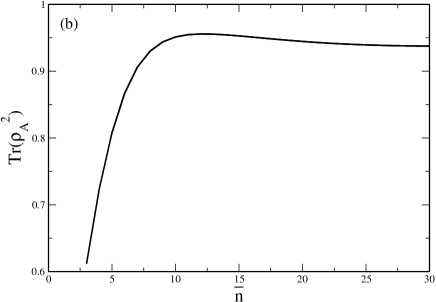
Figure 3: a) Quality factor of the atomic beam $\mathcal{M}^{2}$ as a function of the average photon number $\bar{n}$ for focusing of a Cesium atom in the thin lens regime. b) Trace of squared reduced density matrix of atom $Tr(\hat{\rho}_{A}^{2})$ as a function of the average photon number $\bar{n}$ for focusing of a Cesium atom in the thin lens regime. We see that its purity increases when the average photon number increases and this is a manifestation of the atom-field disentanglement and represents the classical limit of the field. In a similar way, the increasing of the coherence with an increasing average photon number in (a) can also be considered as a manifestation of the atom-field disentanglement and consequently represents the classical limit of the field.

IV Conclusions

Encouraged by the recent success of the experimental measurement of the Gouy phase for matter waves cond ; elec1 ; elec2 proposed in Paz2 for first time, we revisit the focusing of the atomic beam, i.e., consider a quantum lens in order to explore other essentially quantum features of the process. One of then has to do with multiple foci which reflect the granular nature of the cavity field, studied several years ago by Averbukh et al and Orzag et al Schleich1994 . We therefore focus our attention in the atom-field entanglement and discuss how this effect alters a measurable quantity, i.e., the atomic beam covariance matrix and show that a direct consequence of this entanglement is given by the purity loss of one of the degrees of freedom. We also show that the entanglement properties disappear by the enhancement of the average photon number, as to be expected. In the present example, for Cesium atoms the “classical limit” is reached around $\bar{n}\geq 10$ depending on details of the atom-field dynamics during the interaction time which preserve the dispersive limit such as the detuning and the number of photon in the field state.

References

- (1) I.S. Averbukh, V.M. Akulin, W.P. Schleich, Phys. Rev. Lett. 72 (1994) 437; B. Rohwedder, M. Orszag, Phys. Rev. A 54 (1996) 5076.
- (2) T.W. Hänsch, A. Schawlow, Opt. Commun. 13 (1975) 68; D. Wineland, H. Dehmelt, Bull. Am. Phys. Soc. 20 (1975) 637; A. Ashkin, Phys. Rev. Lett. 40 (1978) 729; C. S. Adams, E. Riis, Prog. Quant. Electr. 21 (1997) 1.
- (3) F. Schmidt-Kaler, T. Pfau, P. Schmelcher, W. Schleich, New Journal of Phys. 12 (2010) 065014.
- (4) L. G. Gouy, C. R. Acad. Sci. Paris 110 (1890) 1251; L. G. Gouy, Ann. Chim. Phys. Ser. 6 24 (1891) 145; H. C. Kandpal, S. Raman, R. Methrotra, Optics and Lasers in Eng. 45 (2007) 249; A. B. Ruffin, J. V. Rudd, J. F. Whitaker, S. Feng, H. G. Winful, Phys. Rev. Lett. 83 (1999) 341; T. Feurer, N. S. Stoyanov, D. W. Ward, K. A. Nelson, Phys. Rev. Lett. 88 (2002) 257402; F. Lindner, Phys. Rev. Lett. 92 (2004) 113001; T. Klaassen, A. Hoogeboom, M. P. van Exter, J. P. Woerdman, J. Opt. Soc. Am. A 21 (2004) 1689; W. Zhu, A. Agrawal, A. Nahata, Opt. Express 15 (2007) 1995; D. Kawase, Y. Miyamoto, M. Takeda, K. Sasaki, S. Takeuchi, Phys. Rev. Lett. 101 (2008) 050501; A. Wicht, J. M. Jensley, E. Sarajlic, S. Chu, Physica Scripta T102 (2002) 82; P. Cladé et al, Phys. Rev. A 74 (2006) 052109;
- (5) I. G. da Paz, M. C. Nemes, S. Pádua, C. H. Monken, J. G. Peixoto de Faria, Phys. Lett. A 374 (2010) 1660; I. G. da Paz, M.C. Nemes, J. G. Peixoto de Faria, J. Phys.: Conference Series 84 (2007) 012016.
- (6) I. G. da Paz, P. L. Saldanha, M. C. Nemes, J. G. Peixoto de Faria, New Journal of Phys. 13 (2011) 125005.
- (7) A. Hansen, J. T. Schultz, N. P. Bigelow, Conference on Coherence and Quantum Optics Rochester, New York, United States, June 17-20, 2013.
- (8) G. Guzzinati, P. Schattschneider, K. Y. Bliokh, F. Nori, Jo Verbeeck, Phys. Rev. Lett. 110 (2013) 093601.
- (9) T. C. Petersen, D. M. Paganin, M. Weyland, T. P. Simula, S. A. Eastwood, M. J. Morgan, Phys. Rev. A 88 (2013) 043803.
- (10) W.P. Schleich, Quantum Optics in Phase Space, Berlin, Wiley-VCH, 2001.
- (11) B. E. A. Saleh, M. C. Teich, Fundamentals of Photonics, New York, John Wiley et Sons, 1991.
- (12) I. Bialynicki-Birula, Acta Phys. Polonica B. 29 (1998) 3569.
- (13) A.F.R.T. Piza, Mecânica Quântica, São Paulo, Edusp, 2003.
- (14) S. Fengn, H.G. Winful, Opt. Lett. 26 (2001) 485.
- (15) P.R. Berman, Atom Interferometry, San Diego, Academic Press, 1997.
- (16) Y. Qiu, H. Guo, Z. Chen, Optics Communications 245 (2005) 21.
- (17) J.-F. Riou, W. Guerin, Y. L. Coq, M. Fauquembergue, V. Josse, P. Bouyer, A. Aspect, Phys. Rev. Lett. 96 (2006) 070404; F. Impens, Phys. Rev. A 77 (2008) 013619.