TIME-VARYING DYNAMICAL STAR FORMATION RATE
Abstract
We present numerical evidence of dynamic star formation in which the accreted stellar mass grows superlinearly with time, roughly as . We perform simulations of star formation in self-gravitating hydrodynamic and magnetohydrodynamic turbulence that is continuously driven. By turning the self-gravity of the gas in the simulations on or off, we demonstrate that self-gravity is the dominant physical effect setting the mass accretion rate at early times before feedback effects take over, contrary to theories of turbulence-regulated star formation. We find that gravitational collapse steepens the density profile around stars, generating the power-law tail on what is otherwise a lognormal density probability distribution function. Furthermore, we find turbulent velocity profiles to flatten inside collapsing regions, altering the size-linewidth relation. This local flattening reflects enhancements of turbulent velocity on small scales, as verified by changes to the velocity power spectra. Our results indicate that gas self-gravity dynamically alters both density and velocity structures in clouds, giving rise to a time-varying star formation rate. We find that a substantial fraction of the gas that forms stars arrives via low-density flows, as opposed to accreting through high-density filaments.
1. Introduction
Star formation in galaxies proceeds at a leisurely pace: the time to turn all the molecular gas into stars is much longer than the disk dynamical time (Kennicutt, 1998; Leroy et al., 2008). Denoting the dynamical time by , where is the half-light radius of the disk and is the circular velocity of the galaxy, the star formation rate (SFR) is observed to be
| (1) |
with . In other words, were new supplies not available to the disk, it would take roughly 50 dynamical times to deplete the gas.
One can envision extending the relation between the SFR, gas mass, and dynamical time to smaller scales, including giant molecular clouds (GMCs) or star-forming clumps:
| (2) |
where now refers to the SFR in the host GMC (or a smaller feature such as a clump), is the associated total mass (initially all gas), is the free-fall time of the GMC or clump, and is a dimensionless number referred to as the SFR per free fall time, analogous to . The SFR is not to be confused with the star formation efficiency SFE , where is the total stellar mass. The free-fall time is defined as
| (3) |
where is the mean density in the region of interest.
Zuckerman & Palmer (1974) first realized that should all the Galactic molecular gas () collapse in a free-fall time, the expected SFR would be approximately two orders of magnitude higher than the observed Galactic SFR, the observed rate corresponding to 0.02.111The number they quote is 0.13 but they underestimate the total mass of Galactic molecular gas. Because the correct value is , has often been taken as a constant (e.g., Krumholz & McKee, 2005; Krumholz et al., 2012a). Based on the assumption of a static density probability distribution function (PDF) of lognormal form, Krumholz & McKee (2005) predict with little scatter. The theory consists of choosing a critical density above which gas is believed to collapse into stars, and integrating up the density PDF from to infinity, resulting in a stellar mass. This stellar mass is then divided by the volume-averaged free-fall time.
There are reasons to question this simple result and the constancy of . Recent numerical studies (e.g., Klessen, 2000; Dib & Burkert, 2005; Vázquez-Semadeni et al., 2008; Federrath et al., 2008a; Ballesteros-Paredes et al., 2011; Cho & Kim, 2011; Kritsuk et al., 2011; Collins et al., 2012; Federrath & Klessen, 2013) show the emergence of a power-law tail at the high-density end of the density PDF due to gravitationally induced collapse. The idea that gravitational collapse generates high-density tail is bolstered by the observations of extended tails in the column density PDFs in actively star-forming clouds, in contrast to the lognormal PDFs seen in non-star-forming clouds (e.g., Kainulainen et al., 2009; Schneider et al., 2013). This raises concerns for any theory of star formation that employs a static log-normal density PDF.222 An analytic model to explain the evolution of a power-law density tail has been proposed (Girichidis et al., 2014) but the authors assume pressure-free collapse. We show in this paper (and further in Murray & Chang 2014) that there is a close interplay between gravity and turbulence whose pressure input cannot be ignored. Furthermore, observations suggest that there is a wide range in . Mooney & Solomon (1988) find a range in excess of a factor of 100 in the ratio of far-infrared flux (a proxy for the mass of young stars) to CO line flux in a sample of molecular clouds in the Milky Way. Using different probes of the SFR such as counts of protostellar objects (Heiderman et al., 2010; Lada et al., 2010), infrared luminosities of massive clumps traced in HCN (Wu et al., 2010), and free-free emission and far-infrared emission of massive star-forming regions (Williams & McKee, 1997; Murray, 2011, where the former authors use free-free emission and hydrogen recombination lines to estimate the stellar mass of OB associations), other authors find a similar range in , spanning at least two decades.
Using the data in Heiderman et al. (2010) and Lada et al. (2010), Krumholz et al. (2012a) arrive at a different conclusion than the authors of the former two papers. Krumholz et al. (2012a) argue that SFR on GMC () and smaller scales is as slow as the galaxy-wide SFR with a range in of order only a factor of 10. They reason that the spread in shrinks once different free-fall times are taken into account. Krumholz et al. (2012a) conclude that star formation is universally slow at all times and at all scales. The data they consider, however, only pertain to nearby star-forming clouds.
In contrast, Federrath (2013a) considers a larger sample of local clouds and simulation results to find factors of 100 scatter around constant 2%, using the same method as Krumholz et al. (2012a) to take different free-fall times into account.
Simulations suggest that turbulence does not limit the rate of star formation to (e.g., Wang et al., 2010; Cho & Kim, 2011; Padoan & Nordlund, 2011; Bate, 2012; Krumholz et al., 2012b; Federrath & Klessen, 2012; Myers et al., 2014). Padoan & Nordlund (2011) present both hydrodynamic (HD) and magnetohydrodynamic (MHD) simulations of star formation in turbulently stirred isothermal gas. They find rapid star formation, , in simulations with a virial parameter between and ; including the effects of magnetic fields, they find a decrease in the simulated SFR of about a factor of three: –. Krumholz et al. (2012b) include stellar wind in HD simulations and find . Myers et al. (2014) include both stellar wind and magnetic fields to find . When protostellar outflows are important—typically in regions of low-mass star formation—SFE is usually reduced only by factors of 3 (Matzner & McKee, 2000; Hansen et al., 2012; Machida & Hosokawa, 2013; Offner & Arce, 2014; Federrath et al., 2014a).
In this paper we conduct large-scale (16 pc) HD and MHD simulations of star-forming clouds with continuously driven supersonic turbulence. Like previous simulations, we will find large values of . But we will also discover that is not constant with time—we will find that . In fact, this time dependence is evident in the aforementioned simulations (e.g., Figures 5 and 6 of Padoan & Nordlund 2011; Figure 5 of Krumholz et al. 2012b ; Figure 7 of Myers et al. 2014). All these simulations (including ours) are characterized by an initial lull in SFE. This feature was commonly considered a transient borne out of the artificial and sudden inclusion of gas self-gravity. We argue that this interpretation is not correct: the initially slow rate and low efficiency of star formation are direct consequences of the interplay of self-gravity and turbulent pressure. The physical significance of the initial quiescence in SFE was recognized by Cho & Kim (2011) who also find a time-varying and note the role of self-gravity in shaping the turbulent structure of the gas. We will present quantitative analysis to support this assertion. Myers et al. (2014) find that is time dependent in their HD and MHD simulations with decaying turbulence—they further speculate that continuously driven turbulence should suppress the time dependency of . We will show explicitly using continuously driven turbulent simulations that this is not the case.
This paper is the first in a series of four showing that on GMC scales, is neither constant nor small. We find that in gravitationally bound clouds, the SFR increases with time and can reach or higher. In this paper (Paper I), we present the evidence from our numerical simulations while in Paper II (Murray & Chang, 2014), we present an analytical model based on adiabatically heated turbulence (Robertson & Goldreich, 2012) to explain the results of Paper I. In Paper III (E.J. Lee et al., in preparation), we present observational evidence for dynamical star formation using the most complete census of GMCs in the Milky Way to date, and we find that ranges from to . The GMC catalog and the details of its construction are contained in Paper IV (M-A. Miville-Deschênes et al., in preparation).
We follow the practice of others in this field in using the formation and growth of sink particles as a proxy for star formation (Padoan & Nordlund, 2011; Krumholz et al., 2012b; Federrath & Klessen, 2013, e.g.,). This proxy is not exact, since stars, which are hydrostatic objects, form at much higher density and on much smaller scales (of order at most) than are simulated in our simulations or in those just cited—the dynamic range in these simulations is typically no larger than 1000, so in a 1 pc box the smallest resolved scale is at least 1000 times larger than a star. Recent simulations using adaptive mesh refinement have achieved a dynamic range of eight orders of magnitude, e.g., Tomida et al. (2013), large enough to resolve the outer layers of a protostar. However, such simulations run for only hundreds to thousands of years, not nearly long enough to determine an SFR. The reason, of course, is that the dynamical or sound crossing times on the smallest scale are so short.
This paper is organized as follows. In Section 2 we briefly describe our numerical methods. In Section 3 we analyze the results of our simulations. We discuss our results and compare them to previous work in Section 4, and we conclude in Section 5.
2. NUMERICAL METHODS
We use both ENZO (v2.2 development branch; Bryan et al. 2014) and FLASH 4.0.1 to perform our numerical calculations. Hydrodynamical runs solve the continuity and momentum equations, with Poisson’s equation when self-gravity is included:
| (4) |
| (5) |
and
| (6) |
In these equations is the fluid velocity, is the magnetic field, is the identity matrix, and is the gravitational potential. The gas pressure is given by
| (7) |
where the sound speed is taken to be constant. The evolution of the magnetic field is given by
| (8) |
Readers interested in the architecture of ENZO should refer to Bryan et al. (2014); the relevant equations are their (1)–(8) with , (non-cosmological), (no radiation, no heating, no conduction). Our ENZO runs use the Runge Kutta second-order based MUSCL solver with a Harten-Lax-van Leer (HLL) Riemann solver. The FLASH runs use the unsplit solver recently developed by Lee & Deane (2009), with the Harten-Lax-van Leer Contact (HLLC) Riemann solver for the HD case and the the Harten-Lax-van Leer with Discontinuities (HLLD) Riemann solver for the MHD case. We note that the HLL solver is, by construction, more diffusive and does not resolve shocked regions as well as the HLLC solver. While the two codes disagree at a factor of two level on subparsec scales, the global results are in good agreement.
Our simulations start with uniform density and zero bulk velocity with a fixed resolution of . In our fiducial runs, the physical length of the box is set at , and we use periodic boundary conditions. The initial mass density is . The global free-fall time is then . As mentioned above, all our simulations are isothermal at a sound speed . Thermodynamic studies find that molecular clouds can contain significant amount of atomic gas with temperatures ranging from that of cold neutral medium (CNM) and warm neutral medium (WNM), on the length scales and densities similar to our setup (e.g., Koyama & Inutsuka, 2002; Audit & Hennebelle, 2005; Heitsch & Hartmann, 2008; Banerjee et al., 2009; Audit & Hennebelle, 2010; Vázquez-Semadeni et al., 2010; Heiner et al., 2014). Clouds that harbour star-forming clumps may well have temperature variations but as Heitsch & Hartmann (2008) report, the conversion from atomic to molecular hydrogen is a rapid process, and stars form only in the gravitationally bound molecular clumps. Given the same density threshold for star formation, Heitsch & Hartmann (2008) find , similar to what we find (see their Figure 10) in our isothermal models.
In our MHD runs, we set the initial magnetic field to be uniform, pointing in the x-direction, and to have an intensity of 0.49G, yielding an initial , where is the Alfvén speed. At statistical equilibrium, , corresponding to , on the low side but still within the range of observed magnetic field intensity of molecular clouds of similar densities (see Crutcher, 2012, their Figure 6). Our simulated box is magnetically supercritical ( where ) and so are GMCs. For the typical turbulent velocities of Milky Way GMCs and size 100 pc, number densities of are required for virial equilibrium. The maximum possible magnetic field intensity is then (Crutcher, 2012), corresponding to .
Initially, we evolve the gas without any self-gravity and drive turbulent forcing in Fourier space at wavenumbers ( for ENZO) until the gas becomes fully turbulent at the appropriate Mach number , where is the turbulent velocity at the largest scale . In most of our runs, with either code, we employ a purely solenoidal form of turbulent driving. We have also done some runs employing compressive driving. Compressive driving has been shown, e.g., by Federrath & Klessen (2012), to lead to much larger SFRs than does solenoidal driving. We have concentrated on the more conservative form of driving to reduce the amount by which we may be overestimating the SFR, but we also report on the results of simulations with compressive driving.
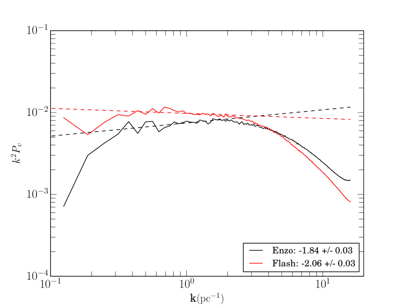
Even in cases where we drive the turbulence on large scales with purely solenoidal driving, on smaller scales the turbulence has both solenoidal and compressive modes. In runs with purely solenoidal driving (using FLASH), the ratio between the turbulent power due to solenoidal and compressive modes is 5:1 at the driving scale, converging to 1:1 at the dissipation scale, i.e., the point where deviates from the flat spectrum seen in Figure 1, at . Similar power ratios have been observed in previous studies such as Federrath et al. (2010b) (see their Figure 14). In our ENZO runs, the power in the compressive mode becomes comparable to that in the solenoidal mode only at scales a few times the grid scale. The difference is likely due to some combination of the different driving scales (ENZO’s driver drives at slightly smaller scales, as noted above) and ENZO’s more dissipative solver.
Away from collapsing regions, the turbulence is found to follow the size-linewidth relation
| (9) |
where , consistent with Burgers turbulence (Burgers, 1948), i.e., high Mach number turbulence, and as observed in GMCs and low-mass star-forming regions by Myers & Goodman (1988). The dynamical time is . The simulation reaches a statistical steady state after 3–5 , whereupon the global virial parameter
| (10) |
reaches, by design, unity. In this expression is the total mass in the box.
The velocity power spectrum of the fully turbulent state is shown in Figure 1. The measured index of this turbulence (1.8–2.1) is close to the expected value for Burgers turbulence and consistent with the value of found above.
Both the sonic length
| (11) |
and the Jeans length
| (12) |
are well resolved in our runs, which have a cell length of .
2.1. Star Formation Prescription
In our fiducial simulations, formation of stars (hereafter “star particles”) is governed by the Truelove criterion: a star is formed at a grid point at which the Jeans length falls below four grid cells (Truelove et al., 1997).333The minimum number of cells to resolve Jeans length has been revised to 30 as four grid cells can overestimate SFE by 11% (Federrath et al., 2014b) and underestimate the magnetic field intensity by at least an order of magnitude (Federrath et al., 2011a). The Truelove criterion is effectively a resolution-dependent density threshold criterion: stars form if the cell has a density above
| (13) | |||||
where is the mean density. The material above this density is collected onto a star particle, lowering the density in the grid cell to the value given in Equation (13). Once stars form, they grow in mass via two channels: accreting gas within Bondi radius and merging with other star particles when they are a half-cell distance away (two-cell distance for FLASH).
For comparison, Padoan & Nordlund (2011) form stars only in grid cells where the density exceeds a fixed threshold of 8000, independent of the resolution. At resolution, this threshold density is about 10 times that specified by the Truelove criterion (Equation (13)). However, we show in Section 3.1 that the mass in star particles, , is independent of the threshold criterion employed.
The default star particle methodology used in FLASH 4.0.1 is described in Federrath et al. (2010a). However, we make some significant modifications to reduce the computational load imposed by the formation of hundreds to thousands of stars. As described in Federrath et al. (2010a), star particles are subcycled via a brute-force algorithm, where is the number of star particles. Computing the interactions between star particles themselves is not generally time-intensive. However, there are force evaluations between the gas and the star particles and vice versa, where is the number of grid points. In addition, during each subcycle step, the particle’s position must be updated across all the operating cores. We have found that handling gas-particle interactions is the slowest step of the FLASH code.
To increase the efficiency of the FLASH code, we change the force evaluation between the gas and the star particles and between the star particles and the gas as follows. First, we compute the force between star particles using the same algorithm. Second, we perform the force evaluation on the gas by the star particles, by mapping the particles to the gas grid and solving the Poisson equation. As the Poisson solver is already executed to compute gas self-gravity, the force evaluation between the star particles and the gas is done with the minimal overhead of mapping the star particles onto the grid. Third, to solve for the force on the star particles by the gas, we solve the Poisson equation purely for the gas without mapping the star particles.
As pointed out by Federrath et al. (2010a), this approach leads to large errors in the dynamics of binary stars integrated over many binary orbital periods. However, we are interested here in the SFR; our tests show little difference between the SFRs obtained using our faster method as compared to Federrath’s method. We caution that the properties of the binary and multiple stars formed, which we do not consider in this paper, will likely be different using the two methods.
3. RESULTS
3.1. Evolution of Star Formation Efficiency
After the turbulence has fully developed, we turn on the effects of self-gravity and star particle formation. The global turbulent velocity power spectrum remains unchanged, as was seen by Collins et al. (2012) and Federrath & Klessen (2013).
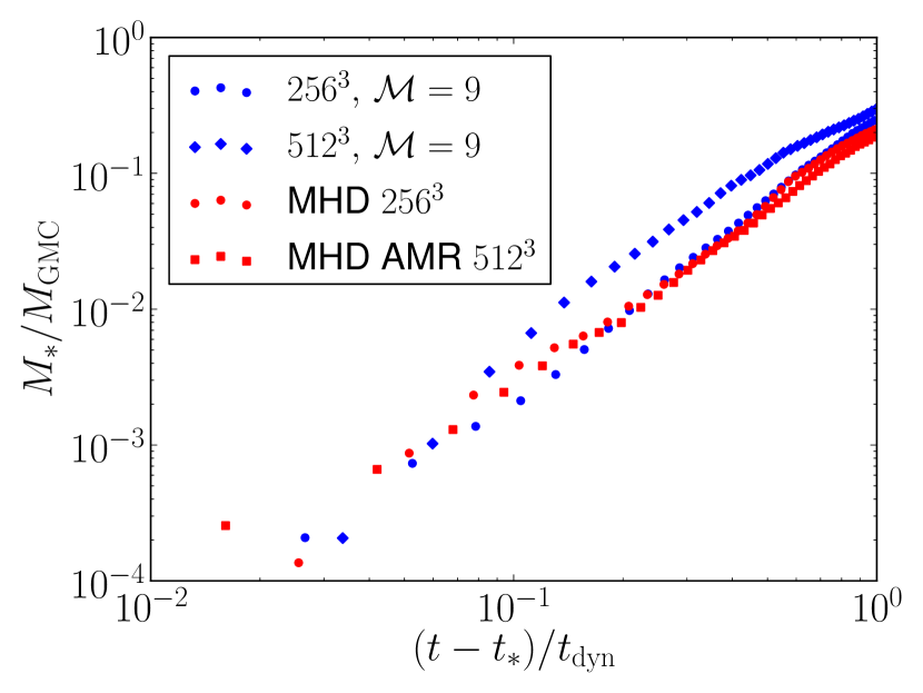
Figure 2 shows how the total stellar mass in the simulation volume, , evolves from the time at which the first star particle forms. In both the pure hydro and MHD runs, we find the total stellar mass is well described by a power law, , with in the range for FLASH (both HD and MHD) and in the range for ENZO. is the total mass (both stellar and gas) inside the box. Including data points at lower steepens the slope because the collapse dynamics is dominated by gas rather than star particles; including data points at higher flattens the slope because stars are closely packed, interrupting the gas accretion. The exact lower and upper limits of the fitting range are not well determined and chosen after visual inspection to avoid obvious breaks in the power law.
This scaling is roughly the same over our rather limited range of different resolutions. We note that depends on the star formation criterion used and the strength of the initial magnetic field, but we find that the power-law index does not depend strongly on .
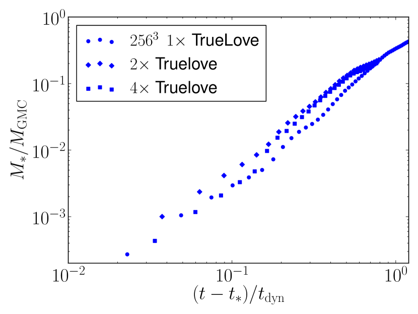
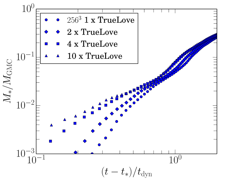
This result is robust to variations in the star formation prescription. Figure 3 shows when we vary the density criterion for star particle formation by scaling it relative to the Truelove criterion (Equation (13)). We have used density thresholds that are 2, 4, and 10 times the Truelove criterion; we find that in all our tests. This explicitly demonstrates that the SFR is independent of the subgrid model we use for the small-scale physics of star formation.
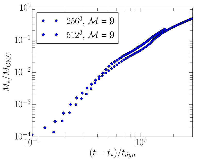
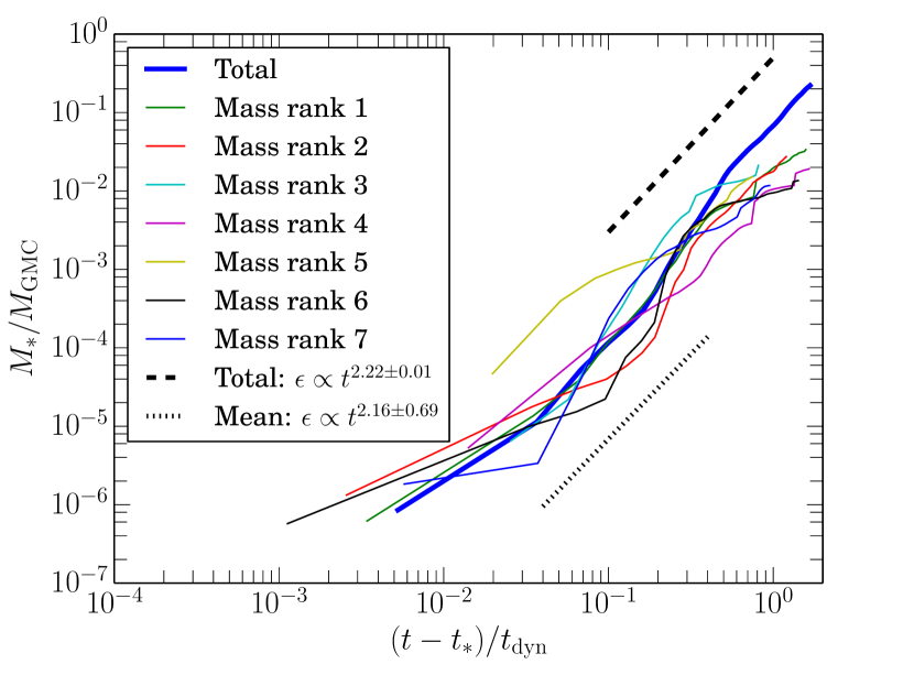
Does hold for an individual star particle as well? We show the mass evolution of individual star particles in Figure 4. Not surprisingly, individual stars have a more stochastic life history than the ensemble of stars, but it is clear that individual stars also tend to grow as . Here we track the seven most massive star particles for a high-resolution run (). Most of the sudden increases in the masses of individual star particles are due to mergers with other star particles.
3.2. Density Probability Distribution Function
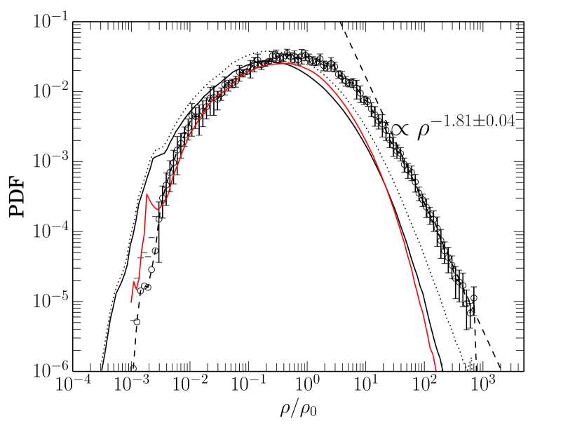
As shown in Figure 5, in gravity-free supersonic turbulence, the volume-weighted density PDF is lognormal, but when self-gravity is included, a power-law tail emerges, corroborating the results of previous works (e.g., Klessen, 2000; Dib & Burkert, 2005; Vázquez-Semadeni et al., 2008; Federrath et al., 2008a; Ballesteros-Paredes et al., 2011; Cho & Kim, 2011; Kritsuk et al., 2011; Collins et al., 2012; Federrath & Klessen, 2013). While this has been noted by many previous authors, only recently was it suggested by Kritsuk et al. (2011) that this power law is due to regions that collapse under self-gravity, and that the power-law exponent is entirely determined by the density profiles of these collapsing regions.
To check this suggestion, in Figure 5 we plot the of regions undergoing gravitational collapse, of regions largely unaffected by the gravity of the star particles, and of the entire simulation box before and after the gas self-gravity is turned on. We define the regions undergoing collapse as spheres each having a radius of centered on star particles. Gas lying outside of these regions is considered noncollapsing. We see that the density PDF of the noncollapsing regions matches well the PDF of the entire box before the inclusion of gravity (i.e., the PDF is lognormal without a power-law tail at high densities). This implies that regions that do not undergo collapse retain the character of pure supersonic turbulence. On the other hand, the density PDFs of collapsing regions show a clear power law at high density. We find this power-law tail to scale as .
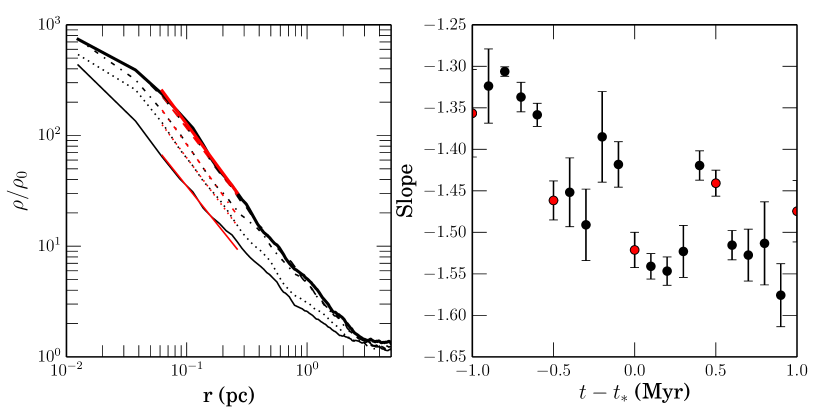
If the density is spherically symmetric and follows a power law , then . Figure 6 shows the evolution of the power-law index of the density profile averaged over 10 massive star particles: starts at before the formation of star particles and then increases to after star formation. The expected range in given the final is 2.07–1.85 which agrees with the numerically determined . The small discrepancy between the expected and observed values is likely due to the combined effect of star particles at different stages of their formation and evolution. Furthermore, a simple power law is only a rough approximation to the run of density; as illustrated in Figure 6, density profiles are not perfect power laws. While our inferred is steeper than the values Kritsuk et al. (2011) report, this is likely because they have higher resolution and they use a different fitting range.
The fact that the density PDF in a self-gravitating gas is lognormal if and only if local density peaks are excised, combined with the very prominent power-law tails seen in the PDF calculated in small volumes around those same peaks and that these slopes of power-law tails are consistent with the slope of the averaged density profile, confirms the suggestion of Kritsuk et al. (2011) that the power-law tail is due to gravitationally induced collapse.
3.3. Importance of Gas Self-gravity
Simulations of star formation must account for several kinds of gravitational interactions: the self-gravity of gas on gas, the self-gravity of stars on stars, and the gravity between gas and stars. Star particle creation routines provide a fourth model for gravity on sub-grid scales. Our sub-grid model is ideally suited to testing the idea that star formation results from collapse of gas in a lognormal density PDF above a density on the scale of the sonic length, as long as the sonic length is resolved.
In this subsection, we systematically turn on and off each of these four kinds of gravitational interactions to determine their relative impact on the time evolution of SFE and the density PDF.
Figure 7 demonstrates that neglecting the gas self-gravity leads to a much slower SFR, roughly by a factor of 10, and a linear mass growth rate with . In contrast, the gravity due to stars does not have such a dramatic effect on the star formation: the rate decreases by less than a factor of two, with an unchanged power-law exponent . Simulations employing compressive turbulence driving tend to have SFE about factors of 10 larger than simulations under solenoidal turbulence (Federrath & Klessen, 2012), a result we reproduce here (left-pointing triangles in the figure). However, Figure 7 shows that even under purely compressive turbulence driving, in the absence of gas self-gravity, SFE remains about a factor of 10 lower than simulations with gas self-gravity under purely solenoidal turbulence.
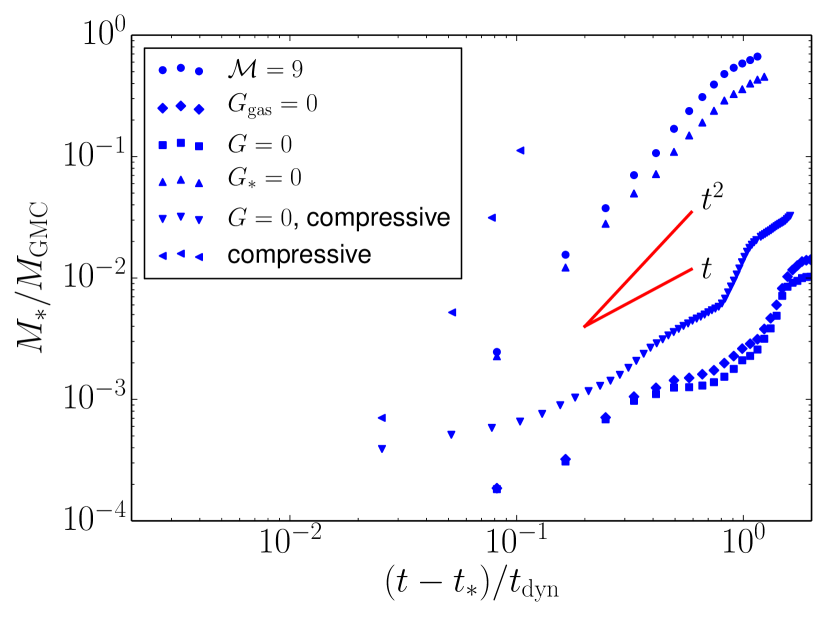
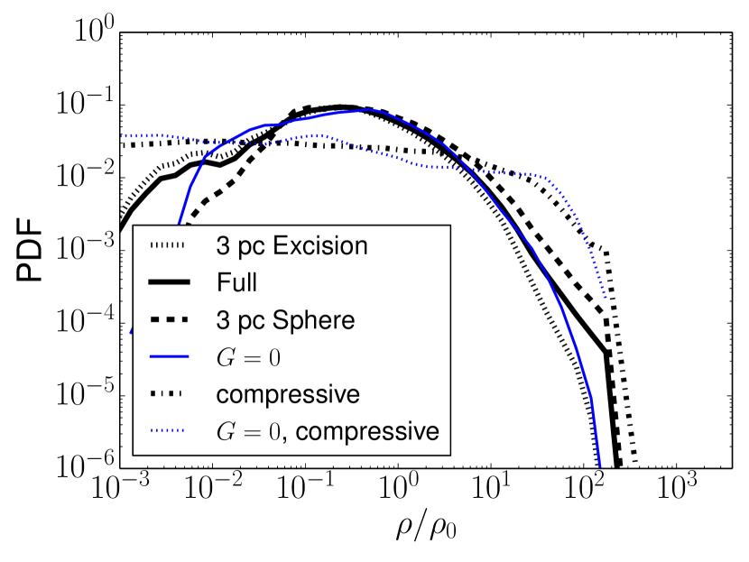
Figure 8 shows that the power-law density tail does not appear in the absence of gas self-gravity in simulations with solenoidal driving, consistent with our contention that the tail is due to gravitationally induced collapse driven by the gas-on-gas potential rather than the star-on-gas potential.
Note, however, that the figure also shows that compressive turbulent driving broadens the lognormal density distribution. The density PDFs of the two compressively driven runs are depicted by the dotted and dot-dashed lines. This broadening occurs whether the gas self-gravity is included or not; because of our limited resolution, it is difficult to determine whether there is a power-law tail to either of these two PDFs. This broadening is reminiscent of that seen in observations of molecular gas compressed by ionization feedback from HII regions (Tremblin et al., 2014). Numerically, the sensitivity of density distribution on the mode of turbulence driving has been extensively studied and discussed by Federrath et al. (2008b) and Federrath et al. (2010b).
While the difference between the PDFs of the two compressively driven simulations is difficult to see in Figure 8, the rapid rate of star formation in the gravity-on case (left-pointing triangles in Figure 7), compared to the gravity-off case, (downward-pointing triangles in that figure) shows that the rate of mass flow from large scales to small scales is far faster in the gravity-on case. We interpret this to mean that the much broader density PDF in compressively driven turbulence is not directly responsible for the more rapid star formation rate seen in previous simulations of star formation in previous work. Instead, it is the increased infall velocity, produced by the initially denser post-shock gas’s self-gravity, that leads to the high SFR, and not the compressive driving by itself. We suspect that our low resolution might play a role in the very strongly enhanced SFR we find in the gravity-on compressively driven case; were we able to follow the flow to yet smaller scales, the enhanced turbulence in the compressively driven case might be seen to slow the infall velocity on those smaller scales, compared to a noncompressively driven case. We are investigating this point further.
These experiments show that gas self-gravity is the primary driver of the rapid SFR seen in our simulations, and of the power-law tails in density PDFs. Models of star formation must, therefore, include not only the small-scale potential produced by stars, but also the large-scale () potential produced by gas. Models that neglect the large scale effects of self-gravity, e.g., those that assume a log-normal density PDF and no feedback effects, will underestimate the SFR by factors of 10 or more.
3.4. Velocity Profiles
We now turn to the velocity profiles around these collapsing regions. In Figure 9, we plot the mass-averaged infall velocity , the free-fall velocity , and the rms velocity
| (14) |
Here measures displacement relative to a reference position .
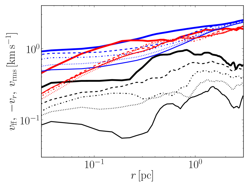
Around density peaks, we find that , flatter than the background turbulent velocity . We attribute the enhanced turbulent velocity and flatter slope in the vicinity of density peaks to the conversion of gravitational potential energy into turbulent energy. The kinetic energy of the bulk inflow of gas also contributes to the driving of turbulence, but as Figure 9 shows, its effect is minimal compared to gravity. The idea that gravitational collapse can drive turbulence has a long history (e.g., Hoyle, 1953; Scalo & Pumphrey, 1982), and it has been seen in recent numerical studies (e.g., Sur et al., 2010; Federrath et al., 2011b). However, in the latter two papers, the fraction of energy going into turbulent motions is small compared to that going into radial infall. In our case, the energy in turbulent motion is substantially larger than that in the radial infall. The difference is likely in the initial conditions: Sur et al. (2010) and Federrath et al. (2011b) start with a smooth, spherically symmetric density distribution with transonic turbulence.
Another way to see that the turbulent velocity is enhanced only near local density peaks is to study the velocity power spectrum around these points. Figure 10 shows the power spectrum calculated in cubes on a side, centered around local density maxima and also around random points away from these maxima. Each power spectrum is calculated after applying a Gaussian window function with variance centered on the point of interest. The velocity power spectra around density maxima have much more power on small scales than either the global power spectrum (Figure 1) or the power spectra calculated in an identical manner around random points in the box.
3.5. Collapse Geometry
Figure 11 shows density slices in - and -planes shortly before the first star forms. The figure illustrates the well-known result that simulated stars form in filaments or sheets, which in this case we define by gas with (colored orange), equivalent to number density , the density of the interstellar medium filaments observed by Peretto et al. (2014). The arrows show the projected velocity of the gas, and illustrate the convergent nature of the flow in the vicinity of the density peaks. The filaments in our simulation have length scale 1–2 pc, width 0.1–0.3 pc, total mass 100–200 (not shown), and velocity dispersion 1–2 (see Figure 9), similar to the properties of the SDC13 infrared dark cloud (see Peretto et al., 2014, their Figures 1, 2, 4 and Table 3), and to the properties of the IC 5146 Herschel filaments (Arzoumanian et al., 2011). Figure 9 shows that the gas inside these high-density structures is by and large bound: the local turbulent velocity around density peaks is at or below the free-fall velocity at all radii at all times, while the bulk velocity is well below the free-fall velocity.
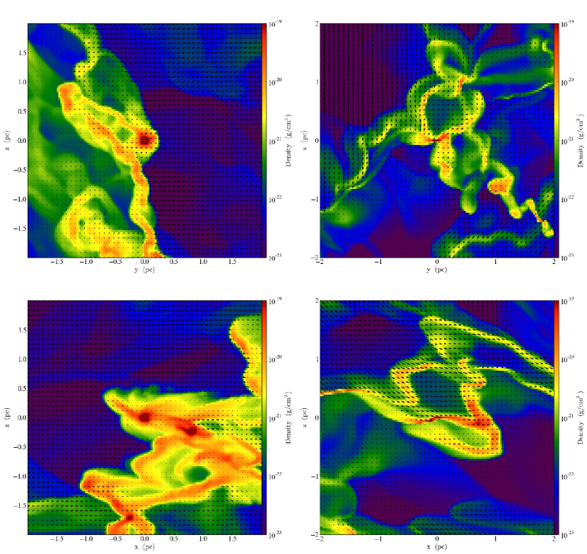
Figure 12 quantifies the source of mass falling onto stars. We plot the mass accretion rate across a spherical shell with radius centered on the local density maximum for 10 star particles at different times. In this plot, we calculate for each cell in the shell and order them by the density in that cell. We then plot the cumulative as a function of density divided by the mean density in the shell, (). The figure shows that half the accretion comes from regions whose gas densities are around or below the mean shell density, whereas only a small fraction of material comes from high-density regions, i.e., filaments.
As a further illustration of this point, we also plot the mass accretion rate for the first star particle, which is shown in the left panels of Figure 11. Once again, the volume average density in the shell is , while the density in the filament is , as can be seen in Figure 11. Only a small fraction of accretion () proceeds through high-density regions, which we are identifying with the filaments seen by Peretto et al. (2014). In fact, 80%–90% of the total mass inside a 2 pc radius sphere centered on the local density maximum resides in structures with .
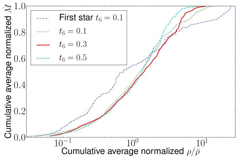
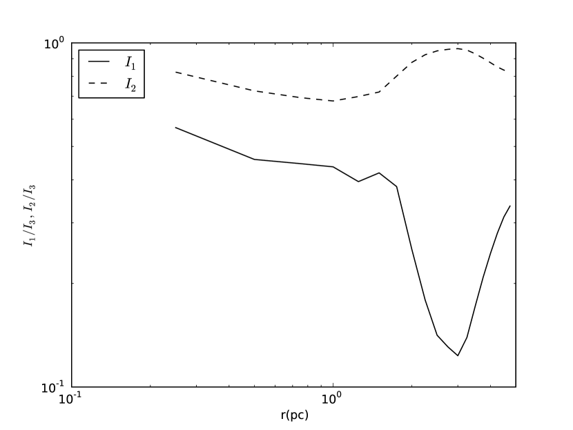
Figure 13 shows moment-of-inertia eigenvalues and , normalized by the third and largest eigenvalue. In the construction of a moment of inertia matrix, positions are measured relative to a star particle. If both and are near 1, the density distribution is spherical; if while is much smaller, the density distribution is filamentary. A flattened filament or sheet would have . Figure 13 shows both and to be near unity near the star particle () but to decrease to for , suggesting that the inner density structure is nearly spherical while the outer density structure is filamentary. There is a hint that again approaches for , possibly reflecting a sheet-like geometry. This confirms the visual impression given by Figure 11.
3.6. Dependence on
Proposed models of star formation predict to decline with increasing (e.g., Krumholz & McKee, 2005; Hennebelle & Chabrier, 2011; Padoan et al., 2012). This is not surprising, since parameterizes the ratio between kinetic energy and gravitational potential energy; we expect objects with low to be bound (and to make stars), while we expect those with high to be unbound and hence to make few stars.
This behavior has been verified in numerical simulations (e.g., Padoan & Nordlund, 2011; Federrath & Klessen, 2012), but exactly how the mass evolution of individual star particles changes with has not been studied in detail.
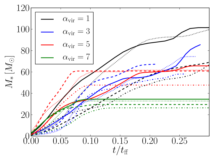
Figure 14 shows the accretion histories of the four most massive stars in each of four runs with different values of the virial parameter. The figure shows that increasing tends to lead to lower mass accretion rates (with substantial scatter). However, the figure also demonstrates that the accretion is shut off before is reached when is large—the green curves () become horizontal at , while the black curves () continue to accrete beyond . Note that both the mass and the time at which accretion halts are similar between all four star particles in the same run. In supervirial clouds, . Because large-scale flows reconfigure the density structure on the dynamical timescale, in high clouds there is less time for star particles to accrete mass than in low clouds. The globally slower SFR at high can then be explained by both the slower accretion rate onto individual star particles and the fact that the supply of gas streaming from large radius toward the star is interrupted when the large-scale turbulent flow varies on a timescale substantially shorter than the (mean density) free-fall time.
4. DISCUSSION
Papers on the SFR in 3D simulations have generally discussed as a constant value (e.g., Padoan & Nordlund, 2011; Bate, 2012; Krumholz et al., 2012b; Federrath & Klessen, 2012; Myers et al., 2014). However, examination of the figures in these papers shows that the stellar mass grows in a nonlinear manner. The figures are consistent with our finding that the SFR rapidly increases with time owing to the effects of self-gravity.
The time-dependence of the SFR has been recognized by Myers et al. (2014) in their simulations, both HD and MHD with stellar feedback. Those authors speculate that the dependency should disappear if turbulence is driven during the gravitational collapse. Our simulations refute this hypothesis: we find to be time-varying in our gravito-turbulent simulations with continuously driven turbulence. Myers et al. (2014) report a global with , while at the same time the same measurement on the most massive stars results in in their HD runs. This is likely because their stellar population has not yet approached a steady-state distribution as shown in their Figure 12.
Simulations that take the formation of and gas accretion onto molecular clouds into account via collision of two WNM flows have also reported SFR to rise with time (e.g., Vázquez-Semadeni et al., 2009) even with the inclusion of stellar feedback (Vázquez-Semadeni et al., 2010; Colín et al., 2013) or magnetic field (Vázquez-Semadeni et al., 2011). Our results and interpretations resonate with the works of Cho & Kim (2011) and Collins et al. (2012), who both suggest that gas self-gravity plays an important role in determining turbulent statistical properties. Through direct comparisons between runs with different kinds of gravitational interactions, as well as close examinations of velocity profiles, we have shown quantitatively that gas self-gravity accelerates star formation and enhances turbulent motion around local density peaks.
Turbulent core-collapse models also predict superlinear stellar mass growth (e.g., in McLaughlin & Pudritz 1997 and in McKee & Tan 2003). While our SFE evolution appears to agree well with the model of McKee & Tan (2003), the turbulent core-collapse model assumes that gas is in hydrostatic equilibrium (HSE). Our density and velocity profiles show that the assumption of HSE is not satisfied in our simulation. What turbulent core-collapse models overlook is that the nature of turbulence is altered by self-gravity; for example the power-law index of the turbulence is altered, as shown in Figure 9. Using the adiabatically heated turbulence model of Robertson & Goldreich (2012), we will show in Paper II that properly accounting for the interplay between gravity and turbulence can explain all the numerical results presented in this paper.
Although the main conclusions of our work are that the SFR and SFE are dynamic and time-varying quantities, we emphasize at the same time that our simulations are compatible with previous work. Indeed, we can reproduce the “constant” calculated by, e.g., Padoan & Nordlund (2011), Krumholz et al. (2012b), and Myers et al. (2014). The value of reported by these papers is found by fitting a straight line to the stellar mass at late times, typically a substantial fraction of a free-fall time after the first stars have formed. Following their recipe, we find similarly large .
Both Krumholz et al. (2012b) and Myers et al. (2014) find that stellar feedback does not significantly alter , suggesting that the forms of stellar feedback they include (protostellar jets, ionized gas pressure, and radiation pressure, calculated using a flux-limited diffusion approximation) do not regulate the SFR at the scale of their simulation (). Even in regions of low-mass star formation where protostellar outflows become important, the SFE reduction factor is only 3 (Matzner & McKee, 2000; Hansen et al., 2012; Machida & Hosokawa, 2013; Offner & Arce, 2014; Federrath et al., 2014a).
In and of itself, rapid local star formation would suggest that the global SFR should be much larger than observed. However, we appeal to other work suggesting that feedback is what determines the global SFR, by regulating the amount of gas in gravitationally bound GMCs (Thompson et al., 2005; Hopkins et al., 2011; Faucher-Giguère et al., 2013).
4.1. Slow Star Formation in Supervirial Gas
The statement that the SFR is of order the cloud mass divided by the free-fall time (Equation (2)) holds for simulations that have global virial parameters of order unity or smaller. Simulations with virial parameters larger than 1 show very different behavior—the SFRs are greatly reduced.
We believe that the low SFRs seen in supervirial simulations reflect the fact that strong turbulence does not allow large-scale steep () power-law density structures to form. Such large-scale structures are a prerequisite for the rapid accretion seen at low . We note that, even in supervirial flows, there are regions of convergent flows in which small-scale bound clumps can form (e.g., Ballesteros-Paredes et al., 1999) and where the large-scale gravitational field plays little or no role. This is essentially how stars form (at greatly reduced efficiency) in our no-gas-self-gravity runs.
If the free-fall time is much longer than the dynamical time, then the newly formed star or cluster will run out of fresh material in a time . To see this, recall Figure 11, which shows that regions of high density occupy little volume. In high- flows, large-scale turbulence strips the outer layers of these enhanced density regions on the dynamical time, limiting the amount of mass that can be accreted onto stars.
4.2. Gravitational versus Turbulent Collapse
Federrath & Klessen (2013) perform simulations similar to ours, but with a broader range of Mach numbers and virial parameters. They obtain many of the same results we do, including very high values of . They emphasize a different aspect of the result, focusing on how variations in the properties of the turbulence affect the SFR: for example, they stress that in simulations with large virial parameters, or noncompressive driving, the SFR is low compared to regions where virial parameter is small or the driving is compressive. We focus on the time evolution of the stellar mass in regions where star formation is proceeding.
We have investigated the relative contribution of turbulence and gas self-gravity to the time evolution of stellar mass in Section 3.1, in particular Figure 7. We show there that turbulence alone—whether purely solenoidal or purely compressive—in the absence of self-gravity, does not drive the rapid star formation seen in simulations that include self-gravity. If high Mach number compressive turbulence were solely responsible for the rapid star formation seen in self-gravitating simulations, then turning off the self-gravity of the gas should not affect the SFR. Furthermore, Figure 8 shows directly that the power-law density tail disappears in the absence of self-gravity, suggesting that the local overdense regions that determine the rate of star formation (not just the seeds of star formation) are generated by gravity. When gas self-gravity is turned off (but when the subgrid star formation routine is still active) star formation does proceed, but at a rate greatly reduced compared to the case where gas self-gravity operates. In addition, SFRs in the no-gas-self-gravity runs do not accelerate with time.
The complementary experiment, where self-gravity operates but there is no turbulent driving, has been reported on many times in the literature. For example, Krumholz et al. (2012b) find that if the gas is initialized with a smooth density distribution and some turbulent velocity field, the time to the formation of the first star is relatively long, but subsequent star formation is exceedingly rapid. By comparison, if the initial velocity distribution is turbulent (initially driven but decays when gravity is turned on) and the emergent density distrubiton is a consequence of initial turbulent driving, the first stars form earlier, but the subsequent SFR grows less rapidly than in the no-turbulence case.
We conclude that while strong turbulence does hasten the initial collapse, it is not the main determinant of the growth rate of stellar mass once star formation begins. Turbulence provides the seeds for local collapse but it is the gas self-gravity that drives accretion onto these seeds. In other words, it is not the number of seeds (or the initial mass of these seeds) that determines the evolution of SFRs; the important determinant is the density structure (and therefore mass) evolution around these individual seeds.
SFRs calculated by integrating over static lognormal density PDFs from a certain critical density (e.g., Krumholz & McKee, 2005) will, therefore, underestimate the true rates. Models of star formation need to properly take into account the dynamical evolution of density PDFs produced by large-scale effects of gravity.
4.3. Collapse on Subgrid, Global, and Intermediate Scales
We distinguish four different scales in our simulations; loss of support against gravity can occur on all four. The smallest scale, which we refer to as subgrid, corresponds to a few to several cell lengths—in our simulations this corresponds to . The loss of support on this and smaller scales is modeled by a star particle creation routine.
The global scale is the size of the box in simulations. In galaxies, we identify the global scale as the local disk scale height, similar to the sizes of the largest GMCs, or, in low-mass star formation regions, the size of the host GMC (which can be substantially below the disk scale height).
We do not see a strong global collapse in any of our turbulent simulations; this is not surprising, since we turn on self-gravity only after establishing fairly strong turbulent motions, with no smaller than one, and then run for a time of order the free-fall time. In simulations with smooth initial density distributions, however, global collapse is observed (e.g., Krumholz et al., 2012b).
Support can also be lost on the local scale whose value depends on the global virial parameter. In most of our simulations, the local scale spans roughly the two decades between the box size and the subgrid scale:
| (15) |
In our simulations, it is this local scale that is relevant for setting the pace of star formation. We have shown that the power-law tail of the density PDF forms on this scale; here the gravitational potential energy liberated from collapse is converted to turbulent energy and flattens the local size-linewidth relation.
For larger values of , the local scale is truncated on the high end by large-scale turbulence, reducing the global SFR dramatically. This ‘supervirial’ truncation scale is the fourth scale we identify.
We have shown that rapid star formation occurs before, and even in the absence of, a global collapse. This result is important: while our simulations lack feedback, we have argued elsewhere that feedback from stars prevents global collapse. That same feedback is likely to cut short the rapid star formation we find here, so that on GMC scales, at least, the fraction of gas turned into stars is well below the or higher levels we find here.
4.4. Comparison to Observations
Krumholz & Tan (2007) and Krumholz et al. (2012a) argue from observations that the SFR per free-fall time on all scales, including scales at or below that of GMCs, is nearly constant and equal to , an order of magnitude below the rates found in numerical simulations.
Most of the GMCs they consider are local clouds lacking massive stars (Heiderman et al., 2010; Lada et al., 2010). Murray (2011), in contrast, finds to range from 0.001 to 0.5 in clouds harboring massive star clusters. Federrath (2013b) finds a similar scatter in using more observations of nearby clouds and clumps. In order to definitively test the constancy of in GMC observations, one must consider all clouds, near or far, actively star-forming or not. This more complete census is what we present in Papers III and IV. We find upward of three orders of magnitude dispersion in and show that our theoretically derived relation fits the observational data well.
The upper end of the observed range in is consistent with the numerical results found here, and the large dispersion seen in likely reflects cloud-to-cloud variations in age and . Our results suggest that supervirial clouds will have low , in agreement with Federrath & Klessen (2012). We test this suggestion observationally in Paper III.
Direct evidence for time-varying was presented by Palla & Stahler (2000); they noted a steeply rising population of younger stars (age 1 Myr) compared to older stars (age 10 Myr) in nearby clusters, interpreting the trend as accelerating star formation. The age distribution in these clusters came into question, however, since sources of error such as differential extinction, stellar photometric variation, and contamination from field stars can also mimic the spread in stellar ages (Hartmann 2001, Lada & Lada 2003, and Hartmann 2003 but see Zamora-Avilés et al. 2012). Other evidence comes from observations of GMCs in the Large Magellanic Cloud. Kawamura et al. (2009) find twice as many clouds with only HII regions than those with star clusters, suggesting that clouds spend more time in the early stages of star formation.
5. CONCLUSIONS
We have argued that the SFR in gravitationally bound objects is controlled by gravity. Examples of such objects include the most massive giant molecular clouds, clumps, and cores. From our finding that stellar mass grows superlinearly with time, most star formation will happen over the 1/10 or 2/10 of a free-fall time. We found that the radial density profile steepens around density peaks at which stars form; at the same time, a power-law tail develops on the high-density end of the lognormal density PDF. Gas self-gravity is responsible for all these changes to the density structure. Gas self-gravity also affects the velocity structure of turbulence, as shown by velocity enhancements near density peaks. In the absence of self-gravity, converging flows also effect changes to the density and the turbulent velocity structures but to a lesser degree.
Unlike the high SFEs seen in our simulations of virialized clouds, supervirial clouds show much slower growth in stellar mass; we have argued that this is because there is not enough time for gas to collapse before turbulence completely alters the density field. Our results show that self-gravity acting on scales larger than 0.1 pc has a direct consequence on cloud density structure, turbulence, and the rate of star formation. From our simulation results as well as the agreement with recent observations, we conclude that SFR is a dynamic, time-varying property, not a constant as previously thought.
References
- Arzoumanian et al. (2011) Arzoumanian, D., André, P., Didelon, P., et al. 2011, A&A, 529, L6
- Audit & Hennebelle (2005) Audit, E., & Hennebelle, P. 2005, A&A, 433, 1
- Audit & Hennebelle (2010) —. 2010, A&A, 511, A76
- Ballesteros-Paredes et al. (1999) Ballesteros-Paredes, J., Hartmann, L., & Vázquez-Semadeni, E. 1999, ApJ, 527, 285
- Ballesteros-Paredes et al. (2011) Ballesteros-Paredes, J., Vázquez-Semadeni, E., Gazol, A., et al. 2011, MNRAS, 416, 1436
- Banerjee et al. (2009) Banerjee, R., Vázquez-Semadeni, E., Hennebelle, P., & Klessen, R. S. 2009, MNRAS, 398, 1082
- Bate (2012) Bate, M. R. 2012, MNRAS, 419, 3115
- Bryan et al. (2014) Bryan, G. L., Norman, M. L., O’Shea, B. W., et al. 2014, ApJS, 211, 19
- Burgers (1948) Burgers, J. M. 1948, Advances in Applied Mechanics, 1, 171
- Cho & Kim (2011) Cho, W., & Kim, J. 2011, MNRAS, 410, L8
- Colín et al. (2013) Colín, P., Vázquez-Semadeni, E., & Gómez, G. C. 2013, MNRAS, 435, 1701
- Collins et al. (2012) Collins, D. C., Kritsuk, A. G., Padoan, P., et al. 2012, ApJ, 750, 13
- Crutcher (2012) Crutcher, R. M. 2012, ARA&A, 50, 29
- Dib & Burkert (2005) Dib, S., & Burkert, A. 2005, ApJ, 630, 238
- Faucher-Giguère et al. (2013) Faucher-Giguère, C.-A., Quataert, E., & Hopkins, P. F. 2013, MNRAS, 433, 1970
- Federrath (2013a) Federrath, C. 2013a, MNRAS, 436, 3167
- Federrath (2013b) —. 2013b, MNRAS, 436, 3167
- Federrath et al. (2010a) Federrath, C., Banerjee, R., Clark, P. C., & Klessen, R. S. 2010a, ApJ, 713, 269
- Federrath et al. (2008a) Federrath, C., Glover, S. C. O., Klessen, R. S., & Schmidt, W. 2008a, Physica Scripta Volume T, 132, 014025
- Federrath & Klessen (2012) Federrath, C., & Klessen, R. S. 2012, ApJ, 761, 156
- Federrath & Klessen (2013) —. 2013, ApJ, 763, 51
- Federrath et al. (2008b) Federrath, C., Klessen, R. S., & Schmidt, W. 2008b, ApJ, 688, L79
- Federrath et al. (2010b) Federrath, C., Roman-Duval, J., Klessen, R. S., Schmidt, W., & Mac Low, M.-M. 2010b, A&A, 512, A81
- Federrath et al. (2014a) Federrath, C., Schrön, M., Banerjee, R., & Klessen, R. S. 2014a, ApJ, 790, 128
- Federrath et al. (2014b) —. 2014b, ApJ, 790, 128
- Federrath et al. (2011a) Federrath, C., Sur, S., Schleicher, D. R. G., Banerjee, R., & Klessen, R. S. 2011a, ApJ, 731, 62
- Federrath et al. (2011b) —. 2011b, ApJ, 731, 62
- Girichidis et al. (2014) Girichidis, P., Konstandin, L., Whitworth, A. P., & Klessen, R. S. 2014, ApJ, 781, 91
- Hansen et al. (2012) Hansen, C. E., Klein, R. I., McKee, C. F., & Fisher, R. T. 2012, ApJ, 747, 22
- Hartmann (2001) Hartmann, L. 2001, AJ, 121, 1030
- Hartmann (2003) —. 2003, ApJ, 585, 398
- Heiderman et al. (2010) Heiderman, A., Evans, II, N. J., Allen, L. E., Huard, T., & Heyer, M. 2010, ApJ, 723, 1019
- Heiner et al. (2014) Heiner, J. S., Vázquez-Semadeni, E., & Ballesteros-Paredes, J. 2014, ArXiv e-prints, arXiv:1403.6417
- Heitsch & Hartmann (2008) Heitsch, F., & Hartmann, L. 2008, ApJ, 689, 290
- Hennebelle & Chabrier (2011) Hennebelle, P., & Chabrier, G. 2011, ApJ, 743, L29
- Hopkins et al. (2011) Hopkins, P. F., Quataert, E., & Murray, N. 2011, MNRAS, 417, 950
- Hoyle (1953) Hoyle, F. 1953, ApJ, 118, 513
- Kainulainen et al. (2009) Kainulainen, J., Beuther, H., Henning, T., & Plume, R. 2009, A&A, 508, L35
- Kawamura et al. (2009) Kawamura, A., Mizuno, Y., Minamidani, T., et al. 2009, ApJS, 184, 1
- Kennicutt (1998) Kennicutt, Jr., R. C. 1998, ApJ, 498, 541
- Klessen (2000) Klessen, R. S. 2000, ApJ, 535, 869
- Koyama & Inutsuka (2002) Koyama, H., & Inutsuka, S.-i. 2002, ApJ, 564, L97
- Kritsuk et al. (2011) Kritsuk, A. G., Norman, M. L., & Wagner, R. 2011, ApJ, 727, L20
- Krumholz et al. (2012a) Krumholz, M. R., Dekel, A., & McKee, C. F. 2012a, ApJ, 745, 69
- Krumholz et al. (2012b) Krumholz, M. R., Klein, R. I., & McKee, C. F. 2012b, ApJ, 754, 71
- Krumholz & McKee (2005) Krumholz, M. R., & McKee, C. F. 2005, ApJ, 630, 250
- Krumholz & Tan (2007) Krumholz, M. R., & Tan, J. C. 2007, ApJ, 654, 304
- Lada & Lada (2003) Lada, C. J., & Lada, E. A. 2003, ARA&A, 41, 57
- Lada et al. (2010) Lada, C. J., Lombardi, M., & Alves, J. F. 2010, ApJ, 724, 687
- Lee & Deane (2009) Lee, D., & Deane, A. E. 2009, Journal of Computational Physics, 228, 952
- Leroy et al. (2008) Leroy, A. K., Walter, F., Brinks, E., et al. 2008, AJ, 136, 2782
- Loken et al. (2010) Loken, C., Gruner, D., Groer, L., et al. 2010, Journal of Physics Conference Series, 256, 012026
- Machida & Hosokawa (2013) Machida, M. N., & Hosokawa, T. 2013, MNRAS, 431, 1719
- Matzner & McKee (2000) Matzner, C. D., & McKee, C. F. 2000, ApJ, 545, 364
- McKee & Tan (2003) McKee, C. F., & Tan, J. C. 2003, ApJ, 585, 850
- McLaughlin & Pudritz (1997) McLaughlin, D. E., & Pudritz, R. E. 1997, ApJ, 476, 750
- Mooney & Solomon (1988) Mooney, T. J., & Solomon, P. M. 1988, ApJ, 334, L51
- Murray (2011) Murray, N. 2011, ApJ, 729, 133
- Murray & Chang (2014) Murray, N. W., & Chang, P. 2014, ArXiv e-prints, arXiv:1407.6373
- Myers et al. (2014) Myers, A. T., Klein, R. I., Krumholz, M. R., & McKee, C. F. 2014, MNRAS, 439, 3420
- Myers & Goodman (1988) Myers, P. C., & Goodman, A. A. 1988, ApJ, 329, 392
- Offner & Arce (2014) Offner, S. S. R., & Arce, H. G. 2014, ApJ, 784, 61
- Padoan et al. (2012) Padoan, P., Haugbølle, T., & Nordlund, Å. 2012, ApJ, 759, L27
- Padoan & Nordlund (2011) Padoan, P., & Nordlund, Å. 2011, ApJ, 730, 40
- Palla & Stahler (2000) Palla, F., & Stahler, S. W. 2000, ApJ, 540, 255
- Peretto et al. (2014) Peretto, N., Fuller, G. A., André, P., et al. 2014, A&A, 561, A83
- Robertson & Goldreich (2012) Robertson, B., & Goldreich, P. 2012, ApJ, 750, L31
- Scalo & Pumphrey (1982) Scalo, J. M., & Pumphrey, W. A. 1982, ApJ, 258, L29
- Schneider et al. (2013) Schneider, N., André, P., Könyves, V., et al. 2013, ApJ, 766, L17
- Sur et al. (2010) Sur, S., Schleicher, D. R. G., Banerjee, R., Federrath, C., & Klessen, R. S. 2010, ApJ, 721, L134
- Thompson et al. (2005) Thompson, T. A., Quataert, E., & Murray, N. 2005, ApJ, 630, 167
- Tomida et al. (2013) Tomida, K., Tomisaka, K., Matsumoto, T., et al. 2013, ApJ, 763, 6
- Tremblin et al. (2014) Tremblin, P., Schneider, N., Minier, V., et al. 2014, A&A, 564, A106
- Truelove et al. (1997) Truelove, J. K., Klein, R. I., McKee, C. F., et al. 1997, ApJ, 489, L179
- Turk et al. (2011) Turk, M. J., Smith, B. D., Oishi, J. S., et al. 2011, ApJS, 192, 9
- Vázquez-Semadeni et al. (2011) Vázquez-Semadeni, E., Banerjee, R., Gómez, G. C., et al. 2011, MNRAS, 414, 2511
- Vázquez-Semadeni et al. (2010) Vázquez-Semadeni, E., Colín, P., Gómez, G. C., Ballesteros-Paredes, J., & Watson, A. W. 2010, ApJ, 715, 1302
- Vázquez-Semadeni et al. (2009) Vázquez-Semadeni, E., Gómez, G. C., Jappsen, A.-K., Ballesteros-Paredes, J., & Klessen, R. S. 2009, ApJ, 707, 1023
- Vázquez-Semadeni et al. (2008) Vázquez-Semadeni, E., González, R. F., Ballesteros-Paredes, J., Gazol, A., & Kim, J. 2008, MNRAS, 390, 769
- Wang et al. (2010) Wang, P., Li, Z.-Y., Abel, T., & Nakamura, F. 2010, ApJ, 709, 27
- Williams & McKee (1997) Williams, J. P., & McKee, C. F. 1997, ApJ, 476, 166
- Wu et al. (2010) Wu, J., Evans, II, N. J., Shirley, Y. L., & Knez, C. 2010, ApJS, 188, 313
- Zamora-Avilés et al. (2012) Zamora-Avilés, M., Vázquez-Semadeni, E., & Colín, P. 2012, ApJ, 751, 77
- Zuckerman & Palmer (1974) Zuckerman, B., & Palmer, P. 1974, ARA&A, 12, 279