The One-Loop Matter Bispectrum in the
Effective Field Theory of
Large Scale Structures
Raul E. Angulo1, Simon Foreman2,3,
Marcel Schmittfull4, and Leonardo Senatore2,3
1 Centro de Estudios de Fisica del Cosmos de Aragon,
Plaza San Juan 1, Planta-2, 44001, Teruel, Spain
2 Stanford Institute for Theoretical Physics and Department of Physics,
Stanford University, Stanford, CA 94306
3 Kavli Institute for Particle Astrophysics and Cosmology,
SLAC and Stanford University, Menlo Park, CA 94025
4Berkeley Center for Cosmological Physics, Department of Physics,
University of California Berkeley and Lawrence Berkeley National
Laboratory, Berkeley, CA 94720
Abstract
Given the importance of future large scale structure surveys for delivering new cosmological information, it is crucial to reliably predict their observables. The Effective Field Theory of Large Scale Structures (EFTofLSS) provides a manifestly convergent perturbative scheme to compute the clustering of dark matter in the weakly nonlinear regime in an expansion in , where is the wavenumber of interest and is the wavenumber associated to the nonlinear scale. It has been recently shown that the EFTofLSS matches to level the dark matter power spectrum at redshift zero up to Mpc-1 and Mpc-1 at one and two loops respectively, using only one counterterm that is fit to data. Similar results have been obtained for the momentum power spectrum at one loop. This is a remarkable improvement with respect to former analytical techniques. Here we study the prediction for the equal-time dark matter bispectrum at one loop. We find that at this order it is sufficient to consider the same counterterm that was measured in the power spectrum. Without any remaining free parameter, and in a cosmology for which is smaller than in the previously considered cases (), we find that the prediction from the EFTofLSS agrees very well with -body simulations up to Mpc-1, given the accuracy of the measurements, which is of order a few percent at the highest ’s of interest. While the fit is very good on average up to Mpc-1, the fit performs slightly worse on equilateral configurations, in agreement with expectations that for a given maximum , equilateral triangles are the most nonlinear.
1 Introduction
To explore the dynamics that drove the inflationary period, it is necessary to probe a large number of modes. The upcoming release of the polarization data from the Planck satellite will increase the amount of available data by at most a factor of two, which means that our knowledge of inflation will be improved by a similar amount, depending on the quantity being constrained. After this, no significant increase in the number of available modes is expected from the CMB, even though some high- measurement might still contain some interesting information. Notice that this situation applies quite unaltered also in the case in which the recent claimed discovery of primordial modes from the BICEP experiment [1] is confirmed. Such a measurement would indeed imply a discovery that Inflation happened at high energies, but it would not enlighten us in detail on the dynamics that drove inflation, for which we need more modes.
This tells us that it is crucial for the field of cosmology to find ways of accessing more primordial modes. The best option to find more modes in the next decade is from large scale structure (LSS) surveys. It is still unclear how many modes will contain relevant cosmological information, and in particular how many of these modes will be accessible with analytical techniques. In order to address this question, the Effective Field Theory of Large Scale Structures (EFTofLSS) was developed in [2, 3]. The EFTofLSS is different from all former available approaches, such as SPT [4] or RPT [5], for the fact that it acknowledges that analytical predictions cannot be made to arbitrarily small scales where the dynamics is completely nonlinear. The effect of short scales on long modes is encapsulated in a series of terms in the equations of motion of the long modes, whose numerical coefficients are not known, and need to be fitted to data or to -body simulations. The role of these additional terms is to compensate for any erroneous dependence on short distance physics that appears when performing calculations in perturbation theory. This is what, in the context of particle physics, goes under the name of renormalization, which is why these additional terms that appear in the equations of motion are often referred to as counterterms.
As described in [6, 7], after the inclusion of these counterterms and after renormalization, perturbation theory amounts to an expansion in the parameters: and . These are defined as
| (1) | |||
where is the linear dark matter power spectrum. represents the effect of tidal forces on a given region, while accounts for the short distance displacements. Both of these scale proportionally to powers of , where is a wavenumber related to the nonlinear scale 111We give a precise definition of later in the text. The place where the EFTofLSS ultimately fails is related to by order one factors that cannot be reliably estimated without detailed calculations. This scale might actually be considered as the true nonlinear scale of the universe, but, as typical for scales where the theory is strongly coupled, it is impossible to determine them without order one ambiguity unless one performs very high order calculations.. In the most common treatment, the so-called Eulerian one, we expand also in the effect of the long distance displacements , where
| (2) |
As described in [7], it is not possible in general to expand in , as for the modes of interest this parameter is of order one in our universe. However, there are some quantities, so called IR-safe, for which the effect of almost cancels out completely, leaving only a small effect connected to the Baryon Acoustic Oscillations. In general, to deal with the effects related to , a resummation of the IR-modes needs to be performed, as it was done in [7]. After this is done, the expansion parameters in the EFTofLSS remain only and , which are smaller than one for . This means that, apart for non-perturbative effects that dominate at very small distances, perturbation theory with the EFTofLSS is manifestly convergent.
So far, the EFTofLSS has been used to predict the power spectrum of dark matter at redshift zero. The results have been incredibly encouraging. The results at two loops [8], after IR resummation [7], agree at 1% with -body simulations to the remarkably high wavenumber of Mpc-1. This represents an improvement of about a factor of six in wavenumber with respect to former analytic techniques, such as SPT. Since available modes scale as the cube of the maximum wavenumber that can be predicted, , these results tell us that there is potentially a factor of about 200 more modes that are amenable to an analytic treatment in next generation LSS surveys than previously believed 222Of course this is a naïve extrapolation of the results obtained at . A more careful estimate would require performing the same study at all redshifts, that we defer to an upcoming paper [9].. Such a potentially picture-changing result makes it very important to check if a comparable improvement persists for every observable. In [7], the momentum power spectrum, which is not an IR-safe quantity, was computed at one loop, where it was shown that, without the need of fitting any additional parameter, the prediction for the momentum showed a gain in the UV reach that was comparable to the one seen for the matter power spectrum, with percent agreement up to Mpc-1. At this point it is tempting to see if a similar improvement holds for higher -point functions. The easiest one is the bispectrum at one-loop, which is the subject of study of this paper.
2 Formulas for One-Loop EFT Prediction
We wish to obtain a prediction for the matter bispectrum , defined by
| (3) |
where the Dirac delta function is written with a subscript to distinguish it from the matter overdensity . Note that, by translation and rotation invariance, the bispectrum is a function of the magnitudes of three wavevectors that add to form a triangle in momentum space, and does not depend on the specific orientation of the triangle. The bispectrum also depends on the time of observation, but in this work we are only concerned with the predictions at , so we will suppress the time-dependence in what follows.
App. A reviews the generic method for solving the equations of motion for and the velocity field and thereby deriving expressions for their correlation functions, and also defines the relevant notation for the solutions (most of which will be familiar from the literature involving SPT, e.g. [4]). Using the procedure outlined in this appendix, and also described in [8] (see also [2]), the lowest-order expression for the bispectrum, which we call because it is a tree graph if written out diagrammatically, is found to be
| (4) |
where is the linear matter power spectrum. The next-order corrections to this expression are the one-loop SPT diagrams , discussed in Sec. 2.1, and various counterterms arising from the terms in the effective stress tensor, which have not previously been included in bispectrum calculations and which we discuss in Sec. 2.2.
2.1 The IR-Safe Integrand of
The one-loop correction in SPT is commonly written as the sum of four terms (e.g. [10]):
| (5) |
where
| (6) | ||||
| (7) | ||||
| (8) | ||||
| (9) |
and we have used . However, as described in [11], explicitly for the case of loop corrections to the power spectrum, it is possible and indeed very convenient to group these terms together as a single integrand to avoid possible numerical issues in the evaluation of the integral. These issues could arise from large IR contributions in each diagram that, for IR-safe quantities, cancel in the final answer. To accomplish this, we first need to map each potential IR divergence 333These potential IR divergences will become true divergences in a no-scale universe () with , and therefore the IR-safety procedure is absolutely necessary to obtain sensible results from the loop integrals in this case. In CDM, the linear power spectrum has a much steeper slope in the IR ( as ), which ensures IR convergence. However, this steepening happens only for Mpc-1, which means that for the ’s of interest here, there will be large contributions peaked at from each diagram that would cancel in the complete computation and therefore pose, at least potentially, a numerical challenge. The IR-safe integrand is automatically well behaved in the IR and so there is no large contribution from IR modes. We have checked in the two-loop power spectrum that the IR-safe integrand leads to a much stronger numerical efficiency [11, 8]. We expect this to be the case also for the bispectrum, even though we have not compared the performance of the IR-safe integrand directly for this case. in momentum space to the origin (). These potential divergences are located at points where the argument of a factor of can approach zero, keeping the external momenta fixed at some nonzero values.
In and , the only point where this can occur is , so no re-mapping is necessary. In , if we examine the first permutation of external momenta that is explicitly written above, there are potential divergences at and ; the second point can be mapped to the first one by the following manipulation, where (which also depends on the external momenta, but we suppress that dependence here) refers to the integrand of :
| (10) |
where we have used the symmetry of under the substitution . An analogous manipulation must be applied to each of the other 5 permutations of external momenta.
The case of is more complicated, for two reasons. The first is the fact that divergences can occur at three locations (, , and ), and the last two must be mapped to the first one. The second is that the form of written in Eq. (6) is proportional to in the limit of the integral, while there are permutations of the other terms that will be proportional to in this limit. Since the IR limits of each integral must cancel with each other regardless of the form of , this means that we might expect to have to manipulate to produce terms proportional to , in addition to re-mapping the potential divergences mentioned above.
Fortunately, these manipulations proceed in a fairly straightforward way. First, let us multiply the integrand of by a sum of products of step functions, like so:
| (11) |
We can now split the integrand into four terms, each multiplying a different product of step functions, and manipulate them so that each term has potential IR divergences only as :
-
1.
:
As or , these step functions evaluate to zero, and therefore this term requires no further manipulation.
-
2.
:
This term is zero when , but not when . However, if we let , then the integrand becomes
(12) which has potential singularities at and , but the step functions evaluate to zero in these limits.
-
3.
:
This term is zero when , but not when , but the substitution changes the integrand to
(13) which again only has potential singularities at , thanks to the step functions.
-
4.
:
After substituting , the integrand is the same in case 3, but with step functions
(14) which evaluate to zero as , and also for , but only if . If , we should repeat the steps above, starting from Eq. (11), but interchanging and and propagating this change through each step. Each of the two cases can then be selected for via appropriate step functions (we will write this explicitly when we present the final expression below).
Thus, we have shown how to write the integrand of in a way that the only potential divergence is located at . Notice also that our manipulations have introduced terms containing in this limit, which will serve to cancel the corresponding terms appearing when external momenta are permuted in the other diagrams.
While the above procedure takes care of the leading potential IR divergences, there are still subleading divergences that would normally disappear after integration over orientations of is carried out. These can be made to cancel prior to integration if an appropriate symmetrization over angles is implemented, but the details of the symmetrization depend on the technique used to translate the integrand into a form that can be evaluated numerically 444For example, we could choose the -axis to lie along , and make the substitution . In this case, there are potentially IR-divergent terms containing , which itself contains the term . This dangerous term will vanish if the integrand is symmetrized in and , but not if the symmetrization is over and , since this would flip the signs of both and . In our own numerical work, we choose to symmetrize in and , and have verified analytically for the case of a scaling universe that all subleading IR divergences cancel as intended when this symmetrization is implemented. .
Thus, the final IR-safe form of can be written in the following way:
| (15) |
where
| (16) | ||||
| (17) |
and
| (18) | ||||
| (19) | ||||
| (20) |
2.2 Counterterms
In the EFTofLSS, the effects of nonlinearities at short distance scales are encapsulated into an effective stress tensor, , on the right-hand side of the Euler equation.555The operator is defined by , which is the quantity that actually appears in the Euler equation, where is the form of the stress tensor more commonly seen in standard treatments of fluids. It is somewhat of an arbitrary choice whether to write an expansion for or ; we find it more convenient to expand the latter, and for brevity we will sometimes refer to as the “stress tensor,” although technically this is a mild abuse of terminology. This stress tensor is written as a double expansion in fields and derivatives, consistent with the symmetries that are relevant at the appropriate scales (namely, rotational invariance and the equivalence principle) The various terms in this expansion add extra contributions to the perturbative solutions for and , which lead to the appearance of counterterms in expressions for various observables.
As noted in [8, 12], there is no obvious separation of timescales between the evolution of short and long modes of the density and velocity fields, and therefore may exhibit significant non-locality in time. This non-locality will manifest itself in counterterms that are evaluated at loop level, such as those appearing in a two-loop calculation of the power spectrum. In the tree-level counterterms that we restrict ourselves to in this work, any non-locality in time will only have a very minor effect. Furthermore, since in [8] we found that nonlinear power spectrum data seem to prefer only a mild degree of non-locality at best, we will comment on where this non-locality might play a role, but in concrete calculations we will take the local-in-time limit for simplicity.
The lowest-order term in the stress tensor is the linear one, which in the local-in-time limit looks like a “speed of sound” term: schematically,
| (21) |
At tree-level, this term will contribute two counterterms to the bispectrum (see App. A for details of the derivation), which, when grouped together into a single expression, take the form
| (22) |
where is given by Eq. (65) in App. A. is related to the free parameter (which also enters into the one-loop EFT prediction for the power spectrum) by , while is proportional to a different constant , which itself is equal to times some order-one factor related to the severity of the non-locality in time. Unless the non-locality is very severe, this factor will be very close to one, so the assumption of locality in time (for which exactly) will not have a huge effect.
There are also four other possible tree-level counterterms we can write down, arising from the contribution to the effective stress tensor that is quadratic in the fields. Three of the terms arise from operators like : schematically, we have
| (23) |
where we used Poisson’s equation to trade for in the second line. Recall that we could also have written a linear counterterm involving the velocity divergence:
| (24) |
At linear order, we have that , where with and being the linear growth factor. As usual in SPT, we can rewrite the velocity field as (see Eq. (50) for a more detailed discussion)
| (25) |
So we define the new counterterm as proportional to
| (26) |
which starts at second order in the fluctuations.
These four counterterms take respectively the following form:
| (27) | ||||
where are arbitrary coefficients, each expected to be of order (there are no factors of because these counterterms are associated with loop diagrams that do not contain any trivial angular integrations). Notice that is a linear combination of and
| (28) |
therefore, since and are free parameters, we can neglect from the rest of the paper.
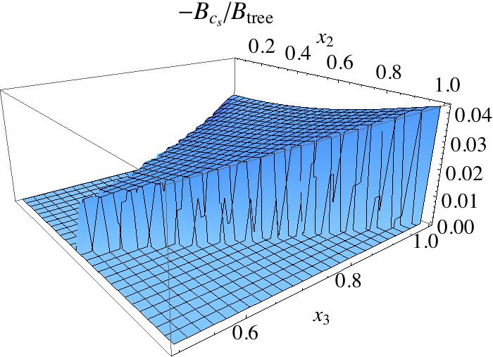
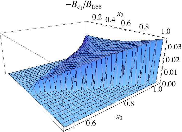
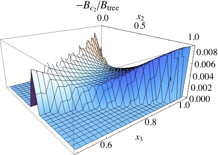
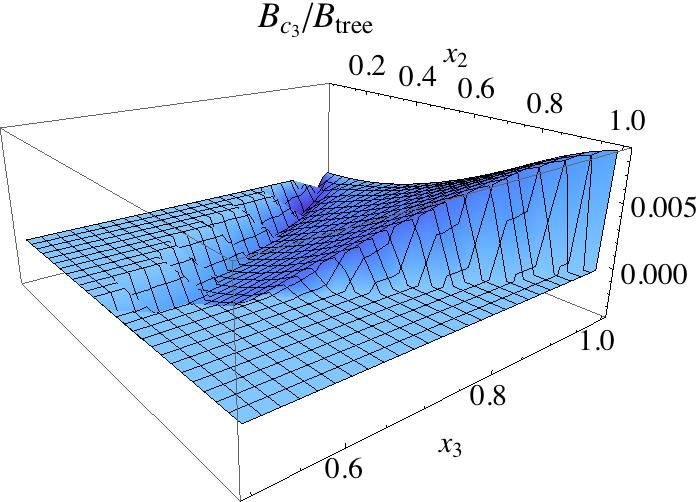
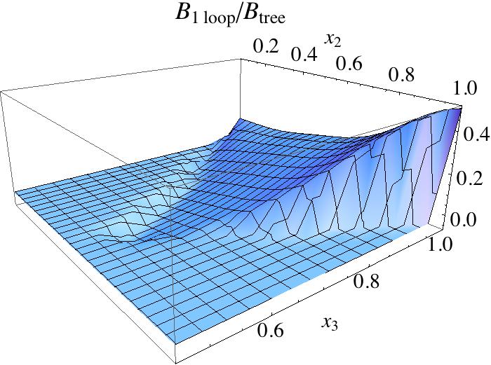
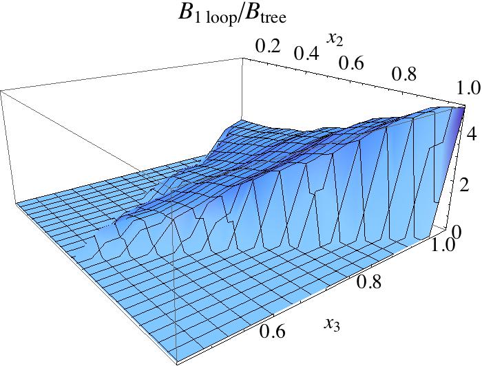
To gain insight into the effect of these terms on the bispectrum in various configurations, in Fig. 1 we plot the ratio of each counterterm to as a function of and for Mpc-1 (the scale-dependence of each term is such that these plots do not change significantly for other values of ). In Fig. 2, we show for Mpc-1 and Mpc-1. To restrict to physical triangles and avoid redundancy in the plots, we only plot in the range . We see from these plots that each term is strongest for equilateral triangles (), and they each become less important for squeezed (, ) and flat () configurations (except for , which tends to peak somewhat in the flat limit). This matches our intuition that of all triangles with one side fixed, equilateral triangles are the most nonlinear, because they are the ones for which each side is closest to the nonlinear scale.
In App. B we show that in the case in which the universe is described by a simple power law, these three counterterms are required to ensure that UV divergences can be cancelled in the bispectrum. This is a sufficient but non-necessary condition that tells that these counterterms should be present in the EFT. It is not a necessary condition because even if these terms were not needed to cancel any UV divergence, they would still be allowed by the symmetry of the problem and therefore should be included.
3 Comparison with Simulations
3.1 N-body simulations
We compare the predictions of the EFTofLSS against the results of a dark-matter only -body simulation. We use the Millennium-XXL (MXXL) simulation [13], which evolved particles inside a comoving cubical region of Mpc a side, from to the present day. The combination of a large volume with a high mass resolution of the MXXL suppresses the effects of cosmic variance and discreteness noise in the bispectrum estimates, therefore allowing a detailed comparison with EFT predictions.
The MXXL simulation was carried out with the following set of cosmological parameters: a matter density of in units of the critical density, a cosmological constant with , a Hubble constant in units of , a spectral index and a normalization parameter for the primordial linear density power spectrum. The initial linear theory power spectrum was computed using the Boltzmann code CAMB [14], and the initial particle positions were determined by adding displacements given by second-order Lagrangian perturbation theory to a random glass-like configuration. Exactly the same power spectrum and cosmological parameters were used in our EFT calculations.
3.1.1 Bispectrum and estimation of errors
In this paper we focus on the bispectrum of the nonlinear mass density contrast at . In order to compute this quantity we first construct a density field by assigning simulation particles onto a cubic grid using a “cloud-in-cells” deposit scheme. We employ a grid of points and then Fast Fourier Transform the respective density field. Finally, we correct for the effects of the assignment scheme by dividing each Fourier mode by the Fourier transform of a cubical top-hat window.
The power spectrum is computed by spherically averaging the amplitude of Fourier modes in annuli of radius . The bispectrum, , is obtained by performing a nested loop over all grid points () and averaging over triangles whose sides satisfy the following condition: , and , where . We note that in subsequent comparisons we discard the imaginary part of the measured bispectrum, and consider only the real one. For these calculations we set Mpc, and .
Specifically, we use triangular configurations with and given by the following list:
| (29) | ||||
| (30) | ||||
| (31) |
For each pair above, we consider 19 different triangles, determined by the angle between and , for which we use 19 equally-spaced values between and . This gives 608 total bispectrum data points, although our method of fitting to triangles with maximum side length less than some cutoff (see Sec. 3.4) means that we only use certain subsets of these data points in our final analysis. In particular, there are 289 triangles with maximum side length less than .
To close this section we discuss the estimation of the error in the measurement of the bispectrum. We adopt the commonly-used expression derived by [15, 16, 10, 17]:
| (32) |
This formula is derived in the Gaussian limit, where should be replaced by , but it seems to be a better approximation for the scales we are interested in here to replace it with . In this expression: is equal to 6, 2, 1 for equilateral, isosceles and general triangles, respectively; is the number of triangles contributing to a given configuration, which, in our case, is directly counted inside the bispectrum code; and . On top of this error, we add an extra 2% error for each bispectrum data point, to account for possible unknown systematic errors in the simulation and in the comparison between simulations and the EFT.
3.2 Determining from the matter power spectrum
The one-loop EFT prediction for the bispectrum will involve the parameter , which can be determined by fitting the one-loop power spectrum prediction to nonlinear data. As discussed in [2, 8, 7], the one-loop power spectrum in the EFTofLSS takes the form
| (33) |
and is expected to be a valid match to the data up to the wavenumber when the two-loop contribution becomes non-negligible. By fitting Eq. (33) to the power spectrum measured from the simulations described in Sec. 3.1, over the range , we find
| (34) |
The upper limit of the fit range is chosen to be roughly where the one-loop prediction begins to deviate significantly from the nonlinear data 666Other choices of the fit range are possible, but the results for the performance of the bispectrum prediction are not significantly affected by this choice. For instance, if is fit over the range , as in [8], we find , but using this value of in the bispectrum prediction only changes the reach of the prediction by 10%, from to . (See Sec. 3.4 for a discussion of how this reach is defined and determined.) Such a change in will of course affect the performance of the power spectrum prediction, but we leave an investigation of this point to future work. .
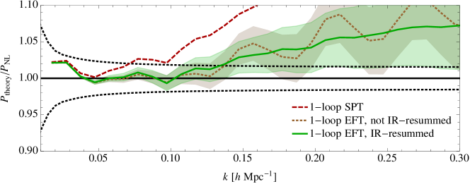
The results of the fit are shown in Fig. 3. In the fit, we use the sampling variance error on , and also add an extra 1% errorbar to account for possible unknown systematic errors in the simulation and in the comparison between simulations and the EFT. As in [8], there are residual oscillations of 2% around the mean of the prediction. These oscillations are due to the effects of bulk flows, and can be eliminated by an appropriate resummation of IR modes, as described in detail in [7] 777We find a way to slightly simplify the numerical implementation of the techniques in [7]. We describe it in App. C. and shown in green in the same figure 888There seems to be a slight systematic offset between the IR-resummed and non-resummed EFT predictions. This is a very small, quite inconsequential, effect, of about 1% in size, whose origin is hard to investigate. We leave this to future work. .
3.3 Bispectrum estimates
In order to utilize the EFTofLSS to make a prediction about the matter bispectrum (or, indeed, any observable), one should have some way of determining which loop corrections and counterterms should be included to reach a given accuracy goal. In [8], estimates were made about the sizes of various terms by treating them in the scaling universe approximation, with an effective and the tilt of the linear power spectrum fit over the range in which the prediction was being made.
We can perform a similar exercise for the bispectrum, in order to estimate when the two-loop correction might become important. The most efficient way to do so is to determine which diagrams will have the largest contribution, and then make a more detailed estimate of their sizes. These diagrams will arise from the correlator , and will scale in the following way when evaluated on equilateral configurations:
| (35) |
The arises from the fact that these diagrams contains two loop integrals that are not nested, which each contribute a factor of (in the language of [8], they are “reducible” diagrams). The 192 is a combinatoric factor related to the number of ways to sew together the diagrams’ internal lines, counted by using diagrams with cubic vertices only (e.g. [5, 18]). The factorials in the denominator arise from integrals over Green’s functions in time: one can consider the Einstein de-Sitter case, when these Green’s functions are roughly the scale factor , and each factor of will involve integrals over these factors, yielding a final prefactor of . The power of counts the number of loops, where is the approximate tilt of in the region we’re making predictions for.
Other two-loop diagrams can be estimated in the same fashion, but they will all either have fewer factors of or else will be more strongly suppressed by inverse factorial factors (for which the combinatorics cannot compensate). We should compare this estimate to , which we write as . We approximate by the size of its largest diagrams (in the sense of having the most factors of along with the smallest amount of combinatorial suppression), which come from and :
| (36) |
For , we count all the permutations in Eq. (22):
| (37) |
Finally, for , we use
| (38) |
To apply these estimates to the universe simulated in Sec. 3.1, we fit a scaling universe power spectrum to the linear spectrum corresponding to the simulations, and find that over the range MpcMpc-1, with and Mpc-1. Therefore, at Mpc-1,
| (39) |
This estimate is uncertain up to factors, but it nevertheless indicates that may strongly limit how far into the UV our prediction can reach. Note that the same estimate applied to the universe from [8], which has a more realistic normalization of the power spectrum and hence a more realistic value of , gives instead of , implying that in the real universe, the reach of the prediction should be farther than what it is in this paper.
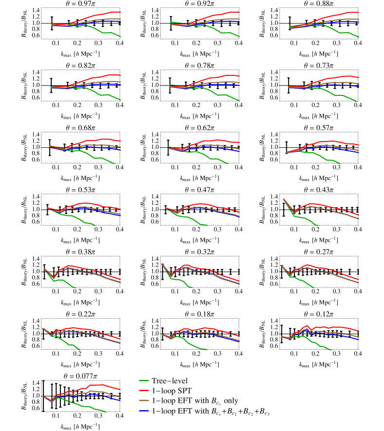
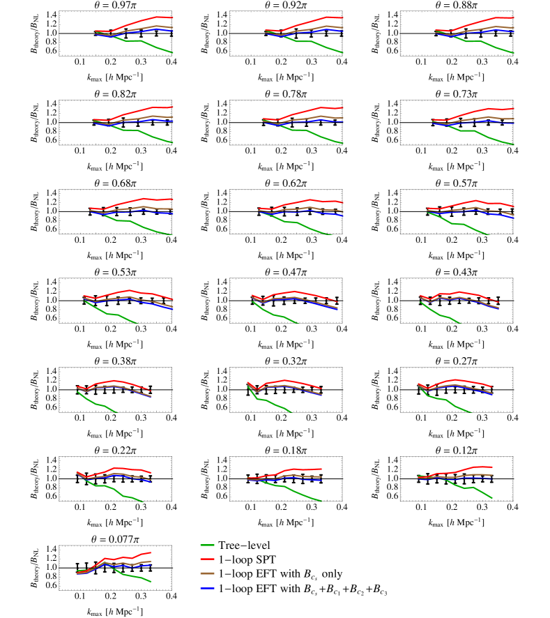
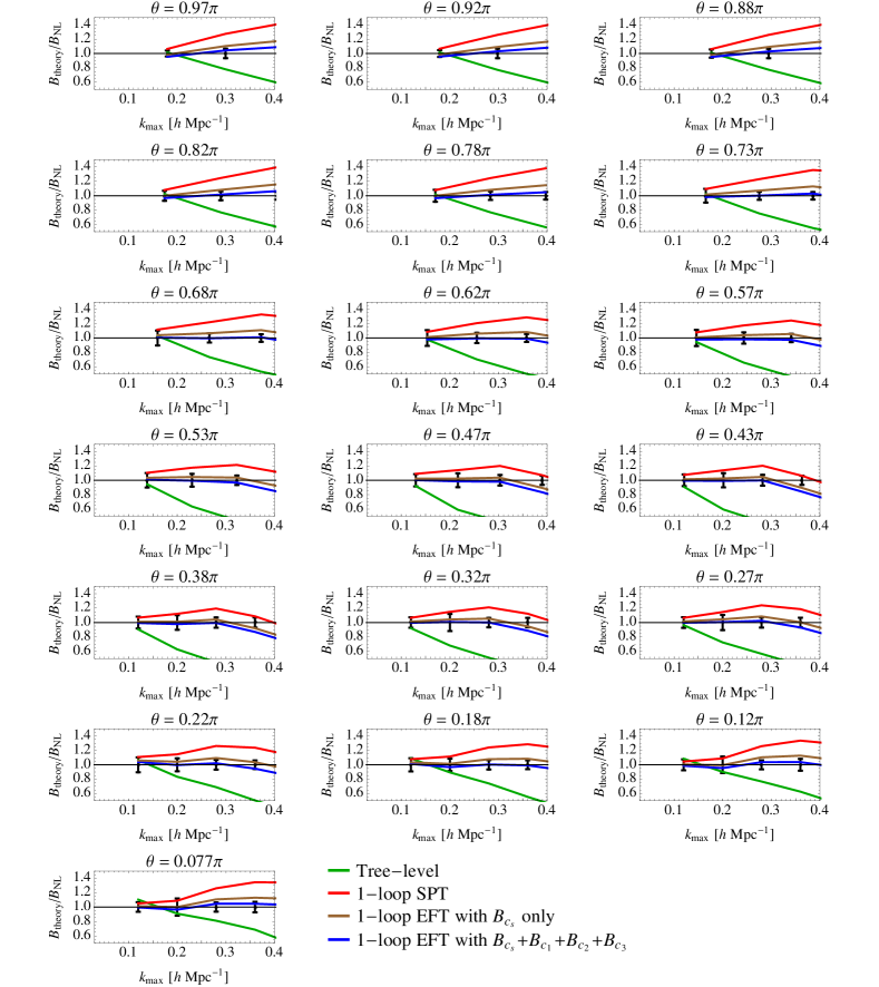
As discussed in Sec. 2.2, there are also three tree-level counterterms besides that could conceivably be important for the one-loop bispectrum prediction. A scaling-universe estimate for the size of each of these terms yields at Mpc-1 999This estimate arises from the following steps. From Eq. (27), we use (40) and comparing this with the estimate for from Eq. (35), we find (41) We expect , and upon plugging this in, along with , Mpc-1, and , we find a value of 0.09 at Mpc-1. We expect similar contributions from and . , implying that the additional counterterms are not parametrically larger than in this region. Since, by definition, our one-loop prediction neglects , this argument implies that we are justified in neglecting these three counterterms as well 101010Notice the following important fact. The current universe can be approximated with the union of two power laws, the transition point being at Mpc-1 [8]. All our estimates so far have been focussed on the most UV region of our fit, where and Mpc-1. For , the linear power spectrum is fitted with a power law with and Mpc-1. Eq. (41) can be applied to ’s below by using and , a slope which is quite steeper than . This means that, as we move towards the infrared, the importance of the additional counterterms relative to grows, and one could potentially find oneself in the situation in which one is allowed to include the additional counterterms without including , because this is justified in some relatively IR region, while not being so in the most UV region. One can easily estimate that we are currently not in this situation for two concurrent reasons: first, by Mpc-1, the ratio from (41) is still sensibly smaller than one; second, as we move to the IR, the numerical data have larger error bars that make the inclusion of the additional counterterms, as well as of the two-loop term, practically unnoticeable, even though their effect might be at percent level. This interpretation is verified by Figures 7, 8 and 9 below. This subtlety will become more apparent after we perform the two-loop computation, something that we plan to do in the future, and when we will have more precise data. In particular, with precise enough data, we expect the fit to improve also at low ’s below , after the inclusion of and of the additional counterterms, a fact that with our available data is not measurable. . In the next section we will check this argument by including these counterterms in a fit to simulation data and examining their affect on the performance of the prediction: if they are smaller than , they should not help the fit too much.
3.4 Results
In this section, we compare various bispectrum predictions to the measurements described in Sec. 3.1. To assess the goodness of fit, we calculate a statistic,
| (42) |
where denotes each triangle of wavevectors with maximum side length less than and is taken from Eq. (32), and then integrate a distribution with the proper number of degrees of freedom from to infinity to find an effective -value, indicating our confidence that the data are described well by each prediction.


In Fig. 4, we display the -values corresponding the one-loop EFT prediction,
| (43) |
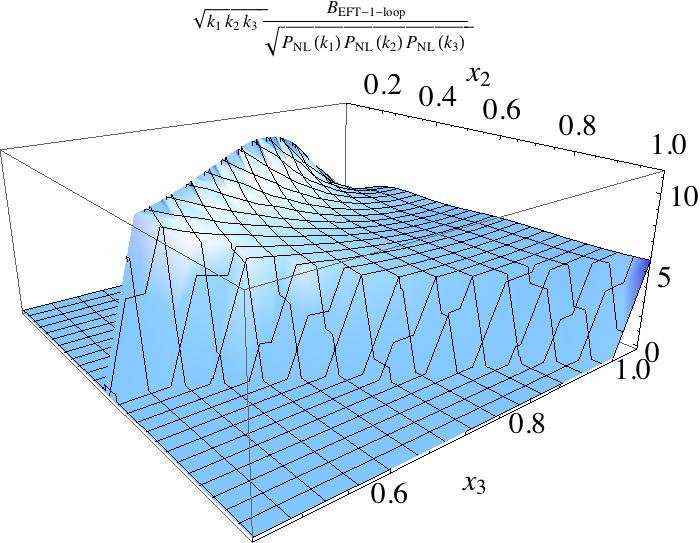
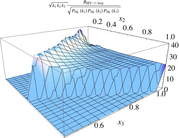
along with the one-loop SPT and tree-level predictions, as a function of in the top panel and in the bottom panel. In the middle panel, we also show the reduced for these predictions. Once is fixed by fitting to the matter power spectrum, the one-loop EFT calculation has no free parameters and extends the range of the prediction compared to one-loop SPT by 65%, which corresponds to a factor of 4.5 more modes whose behavior is reliably captured by the theory 111111Notice that the error bars on the triangles are larger at low ’s that at high ’s, which means that the improvement of SPT with respect to linear theory might be a somewhat overestimated. The bottom panel of Fig. 4 gives a pictorial representation of this improvement. We summarize the shape of the EFT bispectrum for dark matter, that is valid up to Mpc-1, in Fig. 5.


As a check that we are not neglecting any important terms, we also repeat this analysis for the sum of plus the 3 tree-level counterterms we have mentioned earlier:
| (44) |
We simultaneously fit for the values of , , and (while keeping fixed), using all triangles with maximum side length less than some upper limit . The results for various values of are shown in Fig. 6. We find that there is no issue with regard to “over-fitting”: even with the freedom of 3 arbitrary parameters, the fit cannot reach beyond Mpc-1 before becoming much worse at low . Therefore, in this region there must be a higher-order correction, namely and associated counterterms, that contributes significantly to the nonlinear bispectrum.
Furthermore, by examining Fig. 6, we find that the 3 extra counterterms are not able to improve the reach of the prediction into the UV more than about Mpc-1 as compared to the curve. The ratio of and is expected to scale roughly like in this range, implying that if is significant at Mpc-1, it will also be significant at Mpc-1, where fails. Therefore, there is no regime in which the 3 extra counterterms are more important than , and so, as anticipated by our earlier estimates, it is self-consistent to neglect these 3 terms (we must still include , though, because it is enhanced relative to the other counterterms by a factor of ) 121212This interpretation is further confirmed by the fact that the best fit values for the parameters giving rise to the red dotted line in Fig. 6 (which corresponds to a fit using triangles with ) are respectively equal to . An equally good fit is obtained just using the and counterterms, whose have best fit values are . Some of these numbers are quite larger than naively expected, even after considering the small normalization of the shapes of and . This further suggests that these counterterms are trying to compensate for the lack in the theoretical prediction of the two-loop diagram, which is important in that -range. Of course it would be nice to explicitly and more definitively verify this argument with an higher order calculation, something that we leave to future work. .
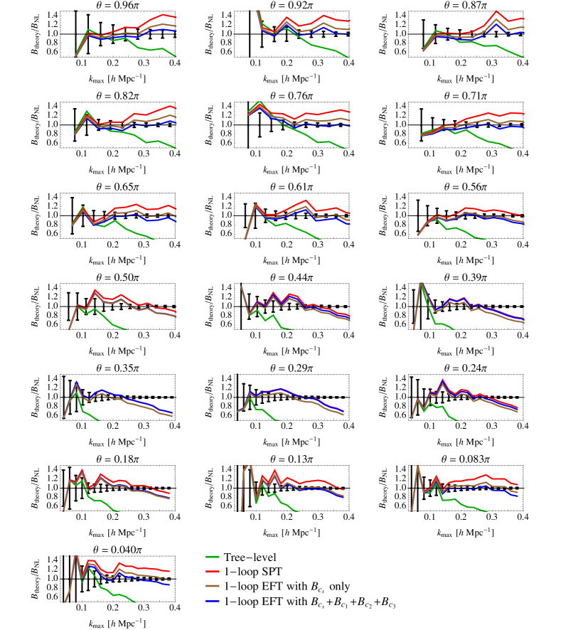
More in detail, Figures 7, 8, and 9 display comparisons of various theory curves with the nonlinear data. There is some configuration-dependence in the maximum wavenumber up to which the EFT prediction can reliably reach, but the average limit of validity is around Mpc-1, similar to the reach of the one-loop prediction for the matter power spectrum with similar error bars. In addition, for equilateral triangles deviates from the data by around 20% at Mpc-1, as predicted (within ) by our prior estimate for .
4 Conclusions
In this paper we have studied the prediction for the equal-time bispectrum of dark matter at redshift at one loop in the EFTofLSS. Since the equal time matter bispectrum is IR-safe, we have contented ourselves with not performing the IR-resummation of [7], which leaves us with small residual oscillations that we will address in future work. Our main interest here was to study the UV reach of the prediction of the EFTofLSS. At one loop, the power spectrum at agrees with numerical simulations at about percent level up to Mpc-1 [2] at one loop131313However, the reach of the one-loop prediction must always be specified along with the precision that is requested of the match between the prediction and nonlinear data. and up to Mpc-1 at two loops [8], after the IR-resummation has been performed [7]. This prediction requires us to fix a parameter, the so called speed of sound , to account for the mistakes from the short distance physics that are accidentally included when doing perturbative calculations. When passing to the bispectrum, we have found that there is no need to include any additional parameter when performing the calculation at one loop. This is so because, at the relevant wavenumbers, the additional counterterms that could be inserted in the bispectrum calculation will contribute in a way that is not safely larger than the two-loop contribution that we do not compute. The only counterterm that we are justified to insert is the term that had already appeared in the power spectrum calculation and had been measured from that observable. For this reason, without any additional parameter to fit, we find that the prediction of the EFTofLSS for the equal-time bispectrum of dark matter at agrees very well with -body simulations up to Mpc-1, given the accuracy of the measurements, which is of order a few percent at the highest of interest 141414The error is dominated by the difference of the power spectrum used in the EFT calculation, where we used the realizations-averaged power spectrum, and the actual ’s simulated by the numerical code. . This is a factor of 65% better than SPT 151515The improvement at one loop with respect to SPT is less strong than in the power spectrum. This might be due to the fact that the relative weight of the counterterms with respect to the loops is diminished as we increase the number of external legs, or to the fact that the errors in the bispectrum measurement are larger at low wavenumbers where SPT fails. . While the fit is very good on average up to Mpc-1, the fit performs somewhat worse on equilateral configurations, in agreement with expectations that for a given maximum , equilateral triangles are more nonlinear than for the other shapes. We should also point out that the simulation we use has a value which is about 10% higher than the current preferred value for our cosmology, so it is expectable that the comparison with observations or simulations with lower or at higher redshifts will show an even better agreement. Still, given the large number of triangular configurations, the average reach of validity of the fit is Mpc-1.
This is a very promising result. The scale up to which we are able to match the data is comparable to the one up to which the EFTofLSS matches numerical data in the power spectrum at one loop. This is an important confirmation of the paradigm of the EFTofLSS, because it is expected that all quantities, when evaluated at the same order in perturbation theory, should match the numerical data to approximately the same wavenumber.
Additionally, it is quite remarkable that we can achieve our result without the addition of a new parameter. The value of is fitted to the power spectrum, and the prediction for the bispectrum follows without any freedom. In fact, we can even ask if the fit can be improved by adding additional quadratic counterterms to the calculation. This is a useful check because there is some uncertainty on the actual size of the various terms, so that it is possible that the additional quadratic counterterms might potentially contribute in a larger way than the two-loop contribution. We instead find that after adding the additional counterterms, the -reach of the fit is improved only slightly, which shows that the two-loop contribution is relevant roughly at the scales where our one-loop calculation fails. Somewhat contrary to what happens for the power spectrum, it is very straightforward to identify the -value when the prediction of the EFT stops matching the data. Finally, we notice that the same parameter determined from the matter power spectrum can predict the momentum power spectrum so that it agrees with the numerical data up to . In other words, the two-loop matter power spectrum, the one-loop momentum power spectrum, and now the one-loop bispectrum are all predicted with only one parameter.
There are a number of ways that we envision to proceed. First, it would be interesting to have more accurate -body simulations, to tighten even more the error bars and understand better the performance of the prediction. Alternatively, and potentially even better, we could perform the EFT calculations directly for the actual realization being simulated by the codes, so that cosmic variance would be made negligible. Second, as it was done for the power spectrum, we would like to extend the calculation to two loops and include IR-resummation. These results obtained in the context of the EFTofLSS keep suggesting that there is a much larger number of cosmological modes that are amenable to analytic techniques. We believe this program is very important to assess what we will learn on primordial cosmology in the next decade, and therefore we are eager to push it forward.
Acknowledgments
Raul E. Angulo and Marcel Schmittfull provided the measurement from the numerical simulations, while the other authors performed the analytic calculations in the EFT and the fits to the data.
We thank Simon White for a brief but intense conversation that helped motivating this project. We thank Daniel Green for initial collaboration. We thank Oliver Hahn, Eiichiro Komatsu, Uroš Seljak, Rashid Sunyaev and Matias Zaldarriaga for interesting conversations. S.F. is partially supported by the Natural Sciences and Engineering Research Council of Canada. L.S. is supported by DOE Early Career Award DE-FG02-12ER41854 and by NSF grant PHY-1068380.
Appendix
Appendix A Solving the Equations of Motion
In this appendix, we review the method to perturbatively solve the equations of motion for and in the EFTofLSS, using the approximation that the time-dependence of each solution is given by an appropriate power of the linear growth factor (normalized to unity at ). If we wish to only make predictions for , it is acceptable to approximate the time-dependence in this way, since the error incurred by this approximation has been shown numerically to be very small [2].161616A more thorough investigation of this point, as well as a formalism that allows computations to be carried out using the full time-dependence, can be found in [18]. In addition, since we only work up to one-loop order, any errors made by this approximation can be partially absorbed into the free parameters we fit to data.
A.1 Loop corrections and linear counterterms
We first review the solutions arising from the standard nonlinear terms ( and , where ) appearing in the equations of motion, as well as from the single linear counterterm () that has previously been considered in studies of the EFTofLSS, as it is the relevant counterterm for the matter power spectrum at one and two loops [2, 8]. We refer the reader to [8, 2] for a more extensive discussion of the motivations and assumptions underlying the formalism we present below.
The starting point is the equations of motion from [8], including only the term from the stress tensor that is linear in , integrated against an unknown kernel that parametrizes the non-locality in time of the coupling between long and short modes of the fields:
| (45) |
where is a parameter inserted to organize the powers of appearing in the solutions we will derive, and where
| (46) |
We use the labelled brackets to mean that we take the Fourier transform of the given function and evaluate it at the momentum : . We use as the argument of to ensure that the equations of motion are diffeomorphism-invariant, and also because the behavior of a mode along its entire past trajectory could in principle have an influence on other modes. However, since we will only consider up to one-loop counterterms in this work, and the difference between and only becomes apparent in two- or higher-loop calculations, we can take . We can also use Poisson’s equation to rewrite in terms of , transforming the second equation into
| (47) |
where
| (48) |
These equations can be solved using the following ansatz:
| (49) | |||||
| (50) |
under the assumptions that and , where . (Recall that these assumptions allow us to solve for the momentum-dependent part of the solution at each order using recurrence relations that do not involve the time variable, as explained in [8].) The -dependent parts of the solutions are written in terms of kernels and in the following manner:
| (51) | |||||
| (52) |
with and written analogously in terms of and . Once , , , and are specified, then any correlation function of or can be calculated up to a specified order. The resulting expression will be in terms of the linear matter power spectrum, defined by
| (53) |
which is calculated numerically by a Boltzmann code such as CAMB [14] and used as an input to the EFTofLSS computation.
Plugging Eqs. (49) to (52) into the equations of motion and collecting terms of order yields the following recurrence relations for and , familiar from SPT (e.g. [4]):
| (54) | |||||
Meanwhile, the terms of order (corresponding to solutions involving a single power of ) give recurrence relations for and , under the assumption that
| (55) |
where
| (56) |
and and are constants. In [8], the values and were used; this choice for arises from the assumption that the coefficient of the counterterm in the matter power spectrum has the same time-dependence as , while the choice for cancels factors of that would otherwise have appeared in the kernels. (Note that changing simply redefines , so we are free to set to a convenient value.) In Eq. (55), leaving arbitrary allows for a more general time-dependence of the counterterm in the power spectrum, as discussed further in [9].171717In a cosmological model in which loop corrections diverge (for example, a scaling universe with sufficiently high tilt), recall that the counterterm in the power spectrum will have two parts: one that depends on the method used to regulate the loop integrals, whose role is to cancel the regulator-dependence (e.g. -dependence in the case of a hard momentum cutoff ) of the result, and another whose role is to capture the finite effects of the UV modes that have been “integrated out” of the theory. In the formalism presented here, this would be incorporated by splitting into two separate functions and , each associated with a different value of and different perturbative solutions. For the realistic cosmology we consider in this paper, however, the loop corrections converge on their own and do not require a regulator, and so we only need to consider and corresponding to the finite counterterm. The resulting recurrence relations are the following:
| (57) | ||||
| (58) |
where
| (59) | |||
| (60) |
The value of can be fixed by examining the lowest-order counterterm appearing in the matter power spectrum,
| (61) |
which involves :
| (62) |
To simplify this expression, we set , implying that
| (63) |
This explicitly shows the relationship between and the time-dependence of the tree-level counterterm in the power spectrum.
Now, to fix the value of , one can utilize the fact that over the range where we expect the one-loop EFT prediction for the power spectrum to be valid, MpcMpc-1, the linear power spectrum resembles that of a scaling universe with tilt . In such a universe, the equations of motion obey a scaling symmetry that uniquely determines the value of to be , and this is also approximately the value that results from a fit of the one-loop EFT prediction to nonlinear power spectra at redshifts [9]. Therefore, in this paper we use in our numerical calculations. Also, dimensional analysis and the presence of a trivial angular integral in determine the following relationship between and the parameter we ultimately fit for, :
| (64) |
As mentioned in Sec. 2.2, the solutions contribute to two counterterms (displayed in Eq. (22) for ) to the bispectrum, arising from the correlators of the form and (plus permutations of external momenta). The second one involves and , while the first one involves , which takes the form
| (65) |
in the local-in-time limit of (for which for all ). In the nonlocal case, extra factors of will appear in , but unless the nonlocality is very severe, will be very close to (see [8] for a more precise statement, involving parameterizing the nonlocality by the power of the growth factor appearing in ).
A.2 Quadratic counterterms
As mentioned in Sec. 2.2, the linear term in does not exhaust the possible tree-level counterterms that can enter into the bispectrum calculation—there are also three independent quadratic terms consistent with symmetries that can be written down, along with one linear combination of fields that only contributes at quadratic and higher order:
| (66) |
Taking the Fourier transform of each term and inserting into the Euler equation in the same way as for the linear term, we obtain the following:
| (67) |
Notice that when Eqs. (49) and (50) are inserted into the last () term, the contents of the square brackets have the same time-dependence at each order.
In principle, from here we could repeat the procedure from App. A.1, deriving solutions analogous to for each of the four new terms shown above. However, in this work we are only interested in tree-level counterterms (for which each will be evaluated on the linear solution ) evaluated at , for which the time-dependence has no effect. Therefore, we can simply read off the new second-order contributions to from the equation above:
| (68) |
Then, by taking the correlation of each term in Eq. (68) with two other linear solutions and symmetrizing over external momenta, we obtain the counterterms listed in Eqs. (27). For example, is obtained from
| (69) |
Appendix B Divergences and Renormalization in Scaling Universes
In this appendix we want to illustrate that in scale-free universes where the linear power spectrum is given by a power law
| (70) |
the one-loop power spectrum and bispectrum present UV divergences. These divergences should, and indeed we show that they can, be cancelled by a suitable chosen combination of the counterterms we have included in the EFT. These are the usual linear counterterm, as well as the three new quadratic ones. This result can be interpreted as a sufficient condition that the EFT counterterms are present and induced by the short distance fluctuations. Notice that it is a sufficient but not necessary condition, as even if the counterterms were not needed to cancel any UV divergence, they would still be allowed on symmetry grounds. Furthermore this calculation can be seen as a further check, together with the verification that IR divergences cancel, that our algebra is correct.
Notice that in a scaling universe, the time dependence of the EFT parameters is completely determined by the scaling symmetry present in these universes. The finite part and the UV divergent part, which represents the proper counterterm, as it literally counters a loop diagram, have different time dependences. In particular, the time dependence of the UV divergent part must be exactly the same as the one of the divergent loops. Since in this section we are interested in showing that the UV divergences can be cancelled, we focus only on the UV divergent part of the counterterms. We will consider only the case, which has just a logarithmic divergence. Higher ’s will have additional subleading divergences that will be very similarly cancelled by higher derivative counterterms that we do not study here.
We start by noticing that the one-loop power spectrum is divergent, the divergence coming from the diagram. This requires a renormalization by using the counterterm, as described in general in [2] and for scaling universes in [21, 11]. We obtain
| (71) |
where as in (64) we have that . Here we take the parameter as we are interested in canceling the UV divergent part of the one-loop diagrams.
Next we move to the Bispectrum. The divergent part is given by:
| (72) | |||
Appendix C A Simplification to the IR Resummation
In [7] it was shown that the IR-resummed expression for the dark matter power spectrum up to order in was given by a convolution integral of the following form
| (75) |
where is the power spectrum evaluated to order expanding both in and . Here the convolution matrix is given by
| (76) |
with is related to the probability for a particle of starting at position and ending up at position :
| (77) |
where is defined in eq. (43) of [7]. In [7], was evaluated from (76) for every and by performing a bi-dimensional Fast Fourier Transform (FFT). It is however possible to alternatively evaluate by performing, for each of interest, a one-dimensional FFT. This can be seen by plugging into (76). The integral can be done leading to a , which in turns allows us to evaluate the integral. We then obtain
| (78) |
Plugging (78) into (75), we can then perform then angular integrals analytically, leaving
| (79) |
where
| (80) |
and where we used that . Specifically, the functions that are needed for the equal-time two-loop power spectrum computation are given by
| (81) | ||||
| (82) | ||||
| (83) |
where
| (84) |
and
| (85) | ||||
| (86) |
given in terms of the spherical Bessel functions . The angular integrals in Eq. (80) can also be performed analytically, leaving a single integral in that can then be evaluated via an FFT at each desired value. After this, the remaining integral in (79) is trivial to carry out numerically. In this work, as in [7], we use .
It is also possible to re-derive this simplification working from the derivation presented [7]. We can start from eq. (44) of [7], that reads:
| (87) |
where is such that the power spectrum to order expanding both in and is given by
| (88) |
It is useful to manipulate the above expression by multiplying by 1 written as
| (89) |
so that, by exchanging with when useful, we can write
Now, as done in [7], we perform the approximation to replace , as this amounts to doing a mistake proportional to the gradient of the IR displacements. We therefore obtain directly Eq. (75), but with the matrix directly in the form (78).
Appendix D Consistency Check using Other Simulations
As a check on our primary results presented in Sec. 3.4, we have also performed the same procedure on a second, independent set of simulations. These simulations are based on three realizations with Mpc and grid points, assuming a flat CDM model with , , , , , and , where ; more details can be found in [22]. These cosmological parameters give, over the range MpcMpc-1, with and Mpc-1.
The matter bispectrum we compare to was reconstructed from these simulations using an expansion of separable basis functions (see [22]), rather than the more traditional methods described in Sec. 3.1, and for this reason, the error estimate in Eq. (32) cannot be straightforwardly applied. Instead, we expect there to be two main contributions to the errorbars: scatter between the three realizations, which can be used as a rough estimate for the cosmic variance, and the fact that we truncate the series of basis functions after a finite number of terms, which introduces a separate systematic error. We estimate the uncertainty incurred by this truncation—specifically, the difference between the exact and the reconstructed from the basis functions—by calculating this difference for , for which we know the exact function. We then estimate the total uncertainty in our measurements of by adding this truncation uncertainty, double the scatter between realizations (we double the measured scatter because three realizations will generally not correctly estimate the cosmic variance, and so we prefer to overestimate it), and an extra 2% systematic error. This is a rather gross estimate of the errorbars, but is still useful as a visual aide to determine whether the theoretical predictions are a reasonable match to the data. However, different triangles will have errors that are highly correlated, since the error on each triangle will arise from combined errors on the measured coefficients of each function in the separable basis, and the reader should keep in mind that we ignore these correlations in our fits and plots.
From there, we follow the same procedure as in Secs. 3.2 and 3.4. Fitting the one-loop EFT prediction to the matter power spectrum yields
| (91) |
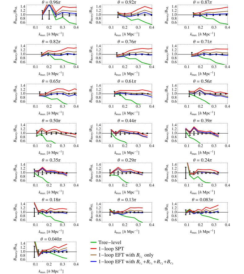
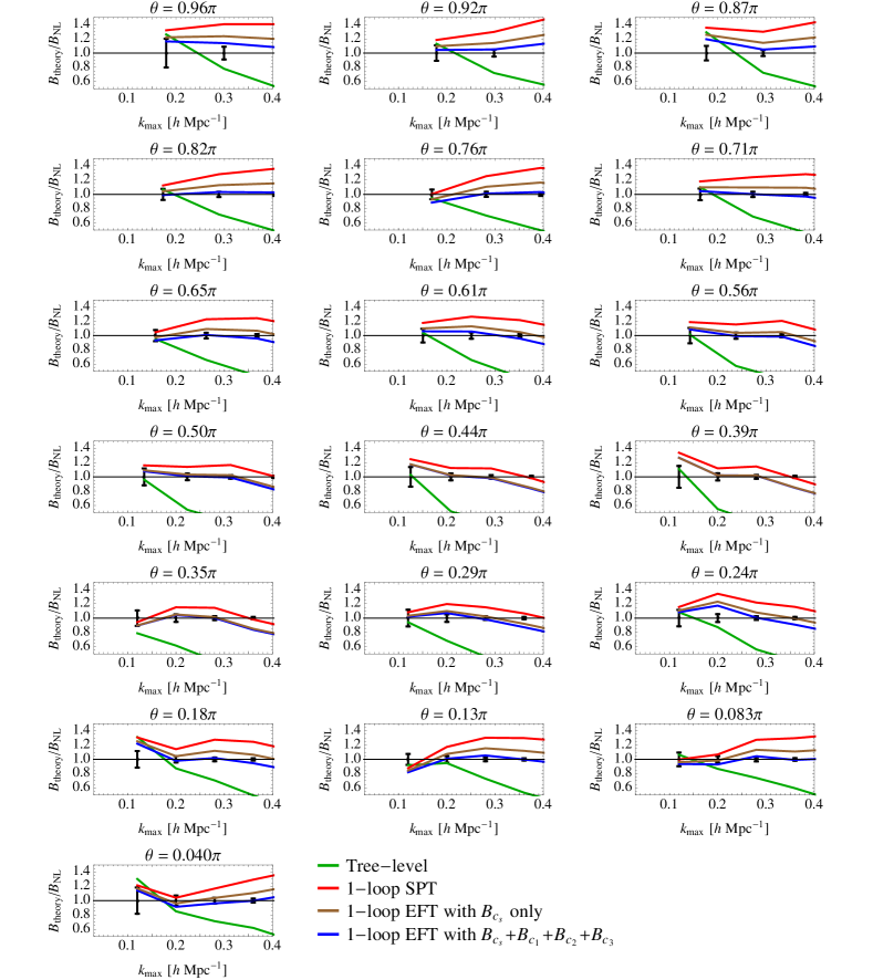
and we use this value, plus values of , , and obtained by fitting the one-loop bispectrum formula to all bispectrum triangles with maximum side length less than Mpc-1, to obtain the results shown in Figures 10, 11, and 12. Once again, the improvement of the EFT prediction over one-loop SPT is evident. The fact that such improvement occurs for two separate sets of simulations demonstrates that the improvement arises from properties of the EFTofLSS, rather than the details of any particular simulation.
References
- [1] P. A. R. Ade et al. [BICEP2 Collaboration], “Detection of -Mode Polarization at Degree Angular Scales by BICEP2,” Phys. Rev. Lett. 112, 241101 (2014) [arXiv:1403.3985] [astro-ph.CO].
- [2] J. J. M. Carrasco, M. P. Hertzberg and L. Senatore, “The Effective Field Theory of Cosmological Large Scale Structures,” JHEP 1209, 082 (2012) [arXiv:1206.2926] [astro-ph.CO].
- [3] D. Baumann, A. Nicolis, L. Senatore and M. Zaldarriaga, “Cosmological Non-Linearities as an Effective Fluid,” JCAP 1207, 051 (2012) [arXiv:1004.2488] [astro-ph.CO].
- [4] F. Bernardeau, S. Colombi, E. Gaztanaga and R. Scoccimarro, “Large scale structure of the universe and cosmological perturbation theory,” Phys. Rept. 367, 1 (2002) [astro-ph/0112551].
- [5] M. Crocce and R. Scoccimarro, “Renormalized cosmological perturbation theory,” Phys. Rev. D 73 (2006) 063519 [astro-ph/0509418].
- [6] R. A. Porto, L. Senatore and M. Zaldarriaga, “The Lagrangian-space Effective Field Theory of Large Scale Structures,” JCAP 1405, 022 (2014) [arXiv:1311.2168] [astro-ph.CO].
- [7] L. Senatore and M. Zaldarriaga, “The IR-resummed Effective Field Theory of Large Scale Structures,” JCAP 1502, 013 (2015) [arXiv:1404.5954] [astro-ph.CO].
- [8] J. J. M. Carrasco, S. Foreman, D. Green and L. Senatore, “The Effective Field Theory of Large Scale Structures at Two Loops,” JCAP 1407, 057 (2014) [arXiv:1310.0464] [astro-ph.CO].
- [9] S. Foreman and L. Senatore, “The EFT of Large Scale Structures at All Redshifts: Analytical Predictions for Lensing,” to appear.
- [10] R. Scoccimarro, S. Colombi, J. N. Fry, J. A. Frieman, E. Hivon and A. Melott, “Nonlinear evolution of the bispectrum of cosmological perturbations,” Astrophys. J. 496, 586 (1998) [astro-ph/9704075].
- [11] J. J. M. Carrasco, S. Foreman, D. Green and L. Senatore, “The 2-loop matter power spectrum and the IR-safe integrand,” JCAP 1407, 056 (2014) [arXiv:1304.4946] [astro-ph.CO].
- [12] S. M. Carroll, S. Leichenauer and J. Pollack, “Consistent effective theory of long-wavelength cosmological perturbations,” Phys. Rev. D 90, 023518 (2014) [arXiv:1310.2920] [hep-th].
- [13] R. E. Angulo, V. Springel, S. D. M. White, A. Jenkins, C. M. Baugh and C. S. Frenk, “Scaling relations for galaxy clusters in the Millennium-XXL simulation,” MNRAS 426, 2046 (2012) [arXiv:1203.3216] [astro-ph.CO].
- [14] A. Lewis, A. Challinor and A. Lasenby, “Efficient computation of CMB anisotropies in closed FRW models,” Astrophys. J. 538, 473 (2000) [astro-ph/9911177].
- [15] J. N. Fry, A. L. Melott and S. F. Shandarin, “The three-point correlation function in an ensemble of three-dimensional simulations,” Astrophys. J. 412, 504 (1993).
- [16] H. A. Feldman, N. Kaiser and J. A. Peacock, “Power spectrum analysis of three-dimensional redshift surveys,” Astrophys. J. 426, 23 (1994) [astro-ph/9304022].
- [17] R. Scoccimarro, E. Sefusatti and M. Zaldarriaga, “Probing primordial non-Gaussianity with large-scale structure,” Phys. Rev. D 69, 103513 (2004) [astro-ph/0312286].
- [18] J. J. M. Carrasco, S. Foreman and L. Senatore, to appear.
- [19] J. Carlson, M. White and N. Padmanabhan, “A critical look at cosmological perturbation theory techniques,” Phys. Rev. D 80, 043531 (2009) [arXiv:0905.0479] [astro-ph.CO].
- [20] T. Hahn, “CUBA: A Library for multidimensional numerical integration,” Comput. Phys. Commun. 168, 78 (2005) [hep-ph/0404043v2].
- [21] E. Pajer and M. Zaldarriaga, “On the Renormalization of the Effective Field Theory of Large Scale Structures,” JCAP 1308, 037 (2013) [arXiv:1301.7182] [astro-ph.CO].
- [22] M. M. Schmittfull, D. M. Regan and E. P. S. Shellard, “Fast estimation of gravitational and primordial bispectra in large scale structures,” Phys. Rev. D 88, 063512 (2013) [arXiv:1207.5678] [astro-ph.CO].