]
www.warwick.ac.uk/andrewgoldsborough
]www.warwick.ac.uk/rudoroemer
Leaf-to-leaf distances and their moments in finite and infinite ordered -ary tree graphs
Abstract
We study the leaf-to-leaf distances on one-dimensionally ordered, full and complete -ary tree graphs using a recursive approach. In our formulation, unlike in traditional graph theory approaches, leaves are ordered along a line emulating a one dimensional lattice. We find explicit analytical formulae for the sum of all paths for arbitrary leaf separation as well as the average distances and the moments thereof. We show that the resulting explicit expressions can be recast in terms of Hurwitz-Lerch transcendants. Results for periodic trees are also given. For incomplete random binary trees, we provide first results by numerical techniques; we find a rapid drop of leaf-to-leaf distances for large .
pacs:
02.10.Ox, 02.10.OxI Introduction
The study of graphs and trees, i.e. objects (or vertices) with pairwise relations (or edges) between them, has a long and distinguished history throughout nearly all the sciences. In computer science, graphs, trees and their study are closely connected, e.g. with sorting and search algorithms Sedgewick and Flajolet (2013); in chemistry the Wiener number is a topological index intimately correlated with, e.g., chemical and physical properties of alkane molecules Wiener (1947). In physics, graphs are equally ubiquitous, not least because of their immediate usefulness for systematic perturbation calculations in quantum field theories Peskin and Schroeder (1995). In mathematics, graph theory is in itself an accepted branch of mainstream research and graphs are a central part of the field of discrete mathematics Rosen (2012). An important concept that appears in all these fields is the distance in a graph, i.e. the number of edges connecting two vertices Leckey et al. (2013); Szekely et al. (2011); Wang (2010). For trees, i.e. undirected graphs in which any two vertices are connected by only one path, various results exist Jacquet and Regnier (1988); Kirschenhofer et al. (1989, 1994), for example, that compute the distance from the top of the tree to its leaves.
Tree-like structures have recently also become more prominent in quantum physics of interacting particles with the advent of so-called tensor network methods Schollwöck (2011). These provide elegant and powerful tools for the simulation of low dimensional quantum many-body systems. In a recent publication Goldsborough and Römer (2014) we show that certain correlation functions and measures of quantum entanglement can be constructed by a holographic distance and connectivity dependence along a tree network connecting certain leaves Evenbly and Vidal (2011). In these quantum systems, the leaves are ordered according to their physical position, for example the location of magnetic ions in a quantum wire. This ordering imposes a new restriction on the tree itself and the lengths which become important are leaf-to-leaf distances across the ordered tree. We emphasize that these distances therefore correspond to quite different measures than those studied in the various sciences mentioned before. We also note that in tensor networks the leaf-to-leaf distance is referred to as the path length Evenbly and Vidal (2011), but in graph theory this term usually refers to the sum of the levels of each of the vertices in the tree Sedgewick and Flajolet (2013).
In the present work, we shall concentrate on full and complete trees that have the same structure as regular tree tensor networks Silvi et al. (2010); Gerster et al. (2014). We derive the average leaf-to-leaf distances for varying leaf separation with leaves ordered in a one-dimensional line as shown e.g. in Fig. 1(a) for a binary tree 111This is the information needed by the holography methods used in Ref. Goldsborough and Römer (2014)..
(a)  (b)
(b) 
The method is then generalized to -ary trees and the moments of the leaf-to-leaf distances. Explicit analytical results are derived for finite and infinite trees. We also consider the case of periodic trees. We then illustrate how such properties may arise in the field of tensor networks. Last, we numerically study the case of incomplete random trees, which is closest related to the tree tensor networks considered in Ref. Goldsborough and Römer (2014).
II Average leaf-to-leaf distance in complete binary trees
II.1 Recursive formulation
Let us start by considering the complete binary tree shown in Figure 1(a). It is a connected graph where each vertex is -valent and there are no loops. The root node is the vertex with just two degrees at the top of Figure 1(a). The rest of the vertices each have two child nodes and one parent. A leaf node has no children. The depth of the tree denotes the number of vertices from the root node with the root node at depth zero. With these definitions, a binary tree is complete or perfect if all of the leaf nodes are at the same depth and all the levels are completely filled. We now denote by the level, , a complete set of vertices that have the same depth. These are enumerated with the root level as . We will refer to a level tree as a complete tree where the leaves are at level . The leaf-to-leaf distance, , is the number of edges that are passed to go from one leaf node to another (cp. Figure 1(a)).
Let us now impose an order on the tree of Figure 1(a) such that the leaves are enumerated from left to right to indicate position values, , for leaf . Then we can define a leaf separation for any pair of leaves and . This is equivalent to the notion of distance on a one-dimensional physical lattice. Let the length be the length of the lattice, i.e. number of leaf nodes. Then for such a complete binary tree, we have .
Clearly, there are many pairs of leaves separated by from each other (cp. Figure 1(a)). Let denote the set of all corresponding leaf-to-leaf distances. We now want to calculate the average leaf-to-leaf distance from the set . We first note that for a level tree the number of possible paths with separation is . In Figure 1(b), we see that any complete level tree can be decomposed into two level sub-trees each of which contains leaves. Let denote the sum of all possible leaf-to-leaf distances encoded in the set . The structure of the decomposition in Figure 1(b) suggests that we need to distinguish two classes of separations . First, for , paths are either completely contained within each of the two level trees or they bridge from the left level tree to the right level tree. Those which are completely contained sum to . For those paths with separation that bridge across the two level trees, there are of such paths and each path has lengths . Next, for , paths no longer fit into a level tree and always bridge from left to right. Again, each such path is long and there are such paths. Putting it all together, we find that
| (1) |
for and with . Dividing by the total number of possible paths with separation then gives the desired average leaf-to-leaf distance
| (2) |
II.2 An explicit expression
As long as , equation (1) can be recursively expanded, i.e.
| (3a) | ||||
| (3b) | ||||
After such expansions, we arrive at
| (4) |
The expansion can continue while . It terminates when becomes so small such that the leaf separation is no longer contained within the level- tree. Hence the smallest permissible value of is given by
| (5) |
where denotes the floor function. For clarity, we will suppress the dependence, i.e. we write in the following. Continuing with the expansion of up to the term, we find
| (6a) | ||||
| (6b) | ||||
Details for the summations occurring in Equation (6b) are given in Appendix A. From Equation (1), we have , so equation (6b) becomes
| (7) |
Hence the average leaf-to-leaf distances are given by
| (8) |
(a)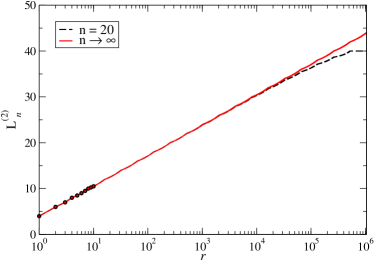 (b)
(b)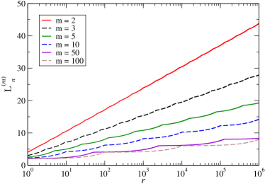
In the limit of for fixed , we have
| (9) |
We emphasize that .
In Figure 2(a) we show finite and infinite leaf-to-leaf distances . We see that whenever , , we have a cusp in the curves. Between these points, the function enhances deviations from the leading behavior. This behavior is from the self-similar structure of the tree. Consider a sub-tree with levels, the largest separation that can occur in that sub-tree is , which has average distance . When becomes larger than the sub-tree size the leaf-to-leaf distance can no longer be but always larger, so there is a cusp where this distance is removed from the possibilities. The constant average distance when is because there is only one possible leaf-to-leaf distance that connects the two primary sub-trees, which is clear from (1).
III Generalization to complete m-ary trees
III.1 Average leaf-to-leaf distance in complete ternary trees
Ternary trees are those where each node has three children. Let us denote by and the sum and average, respectively, of all possible leaf-to-leaf distances for given in analogy to the binary case discussed before. Furthermore, . Following the arguments which led to Equation (1), we have
| (10) |
This recursive expression can again be understood readily when looking at the structure of a ternary tree. Clearly, will now consist of the sum of leaf-to-leaf distances for three level trees, plus the sum of all paths that connect the nodes across the three trees of level . The distances of these paths is solely determined by irrespective of the number of children and hence remains . As before, we need to distinguish between the case when fits within a level tree, i.e. , and when it connects different level trees, . For , there are now such paths, i.e., between the left and center level trees and the center and right level trees. For there are paths. We again expand the recursion (10) and find, with in analogy to (5), that
| (11) |
and
| (12) | ||||
| (13) |
III.2 Average leaf-to-leaf distance in complete -ary trees
The methodology and discussion of the binary and ternary trees can be generalized to trees of children, known as -ary trees. The maximal leaf-to-leaf distance for any tree is independent of and determined entirely by the geometry of the tree. Each leaf node is at depth , a maximal path has the root node as the lowest common ancestor, therefore the maximal path is .
A recursive function can be obtained using similar logic to before. For a given , there are subgraphs with the structure of a tree with levels. When is less than the size of each subgraph (), the sum of the paths is therefore the sum of copies of the subgraph along with the paths that connect neighboring pairs. When is larger than the size of the subgraph (), the paths are all maximal. When all this is taken into account the recursive function is
| (14) |
This can be solved in the same way as the binary case to obtain an expression for the sum of the paths for a given , and
| (15) |
The average leaf-to-leaf distance is then
| (16) |
and
| (17) |
We note that in analogy with Equation (5), we have used
| (18) |
in deriving these expressions. Figure 2(b) shows the resulting leaf-to-leaf distances in the limit for various values of .
IV Moments of the leaf-to-leaf distance distribution in complete m-ary trees
IV.1 Variance of leaf-to-leaf distances in complete -ary trees
In addition to the average leaf-to-leaf distance , it is also of interest to ascertain its variance . Here denotes the average over all paths for given in an -ary tree as before. In order to obtain the variance, we obviously need to obtain an expression for the sum of the squares of leaf-to-leaf distances. This can again be done recursively, i.e. with denoting this sum of squared leaf-to-leaf distance for an -ary tree of leaf separation , we have similarly to Equation (14)
| (19) |
Here, the difference to Equation (14) is that we have squared the distance terms . As before, expanding down to (here and in the following, we suppress the superscript of for clarity) gives a term containing ,
| (20a) | ||||
| (20b) | ||||
As before, details for the summations occurring in Equation (20b) are given in Appendix A. We can therefore write for the variance
| (21) |
Using Equations (LABEL:eqn-mary-ana-Qnrec), (16) and (15), we then have explicitly
| (22) |
and also
| (23) |
(a)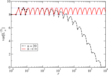 (b)
(b)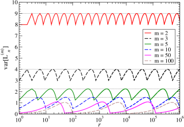
When , , then has a local minima and we find that . Similarly, it can be shown that the local maxima are at , then . These values are indicated in Figure 3 for selected .
IV.2 General moments of leaf-to-leaf distances in complete -ary trees
The derivation in section IV.1 suggests that any -th raw moment of leaf-to-leaf distances can be calculated similarly as in Equation (19). Indeed, let us define as the -th moment of an -ary tree of level with leaf separation . Then , and
| (24) |
Following Equation (19), we find
| (25) |
By expanding, this gives
| (26) |
As before, corresponds to the first value where, for given , we have to use the second part of the expansion as in Equation (25). Hence we can substitute the second part of (26) for giving
| (27) |
In order to derive an explicit expression for this similar to section II.2, we need again to study the final sum of Equation (27). We write
| (28a) | ||||
| (28b) | ||||
| (28c) | ||||
where in the last step we have introduced the Hurwitz-Lerch Zeta function Kanemitsu et al. (2000); Srivastava (2012) (also referred to as the Lerch transcendent Guillera and Sondow (2008) or the Hurwitz-Lerch Transcendent Wolfram Research Inc. (2012)). It is defined as the sum
| (29) |
The properties of are Guillera and Sondow (2008)
| (30a) | ||||
| (30b) | ||||
| (30c) | ||||
Hence we can write
| (31) |
Averages of can be defined as previously via
| (32) |
such that and .
V Complete -ary trees with periodicity
Up to now we have always dealt with trees in which the maximum separation was set by the number of leaves, i.e. . This is know as a hard wall or open boundary in terms of physical systems. A periodic boundary can be realized by having the leaves of the tree form a circle as depicted in Figure 4 for a binary tree.
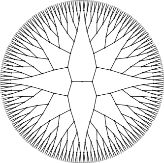
For such a binary tree, only separations are relevant since all cases with can be reduced to smaller values by going around the periodic tree in the opposite direction. Therefore we can write
| (34) |
where and the superscript denotes the periodic case. Note that the case where the clockwise and anti-clockwise paths are the same so only need to be counted once. In the simple binary tree case we can expand this via (7) as in section II.2 and find
| (35) |
with as in Equation (5) and . For every , we have possible starting leaf positions on a periodic binary tree and hence the average leaf-to-leaf distance can be written as
| (36) |
This expression is the periodic analogue to Equation (8). Generalizing to -ary trees, with , we find
| (37) | ||||
| (38) |
The average leaf-to-leaf distance for -ary periodic trees is then given as
| (39) |
To again study the case of , it is necessary to observe how behaves for large and fixed , . When , we have and hence . This enables us to simply take the limits of Equation (39) to give
| (40) |
which is the same as the open boundary case (17). This is to be expected as a small region of a large circle can be approximated by a straight line.
VI Asymptotic scaling of the correlation for a homogeneous tree tensor network
Tree tensor networks (TTNs) are tensor networks that have the structure of a tree graph and are often used to model critical one-dimensional many-body quantum lattice systems as they can be efficiently updated Shi et al. (2006); Tagliacozzo et al. (2009). In principle it is possible to start from a tensor network wavefunction and derive a parent Hamiltonian for which the wavefunction is a ground state Verstraete et al. (2006); Wolf et al. (2006). In the case of homogeneous TTNs the procedure to create such a parent Hamiltonian seems likely to be highly non-trivial and not unique. Here we build such a TTN from the binary tree structure shown in Fig. 1. At each internal vertex we place an isometric tensor Evenbly and Vidal (2009); Goldsborough and Römer (2014) with initially random entries and so-called bond dimension . Using as proxy a spin-1/2 Heisenberg model , with the spin- operator, we perform energy minimisation Evenbly and Vidal (2009); Tagliacozzo et al. (2009) at a bulk site. After each minimization, we replicate the bulk tensor to all other tensors such that every isometry is kept identical Schollwöck (2011). The process is then repeated until convergence (in energy).
A two-point correlation function is calculated Tagliacozzo et al. (2009); Goldsborough and Römer (2014) for all pairs of sites and averaged for all points separated by . The results are given in Fig. 5.
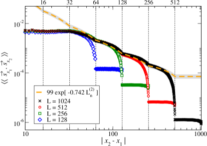
For a homogeneous tensor network, a two-point correlation should scale as Evenbly and Vidal (2011)
| (44) |
where is a constant and is the number of tensor connecting sites and . Hence we expect the asymptotic correlation function to scale as . Figure 5 shows that, away from small separations (e.g. for ), the content of the tensors no longer dominates the structural contribution and exhibits many of the properties we find in Fig. 2(a). The overall form of the long range correlations is a power law. There are also the characteristic fluctuations from the self-similar structure of the tree with cusps at for integer (corresponding to ). When reaching the finite-size dominated regime , we find an approximate constant average correlation. This is smaller than expected from Eq. (9) because the top tensor of the TTN only has and contributes less to the correlation function than the other tensors. We emphasize that we have chosen a low bond dimension so that we can study the asymptotic form of the correlation functions for smaller system sizes.
The form of the correlations expressed in Fig. 5 corresponds to those of a suitable parent Hamiltonian, i.e. one that has a ground state implied by this holographic tree structure. In addition, the results may also be useful for those building TTNs as a variational method for the study of critical systems. The appearance of this form of the correlation for models that do not have a natural tree structure in the wavefunction, such as the Heisenberg model, is an indicator that the chosen is too small to capture the physics of the model. This is similar to the erroneous exponential decay of correlation functions found by DMRG for critical systems with power-law correlations in case of small Schollwöck (2011). In all these situations the structure of the network dominates the value of the correlation rather than the information in the tensors.
VII Leaf-to-leaf distances for random binary trees
In Figure 6(a) we show a binary tree where the leaves do not all appear at the same level , but rather each node can become a leaf node according to an independent and identically distributed random process. Such trees are no longer complete, but nevertheless have many applications in the sciences Sedgewick and Flajolet (2013); Goldsborough and Römer (2014).
(a)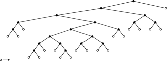 (b)
(b)
Let us again compute the average leaf-to-leaf distance for a given , when all possible pairs of leaves of separation and all possible trees of internal nodes are considered. Here denotes the random character of trees under consideration. For each , there are different such random trees as shown in Figure 6(b). We construct these trees numerically and measure as shown in Figure 7(a) 222We emphasize that this definition of a random trees is different from the definition of so-called Catalan tree graphs Sedgewick and Flajolet (2013), as the number of unique graphs is given by the Catalan number and does not double count the degenerate graphs as shown in the center of the case of Figure 6(b).. For small , we have computed all trees (cp. Figure 7(a)) while for large , we have averaged over a finite number of randomly chosen binary trees among the possible trees (cp. Figure 7(b)).
(a)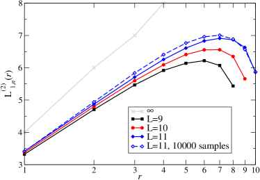 (b)
(b)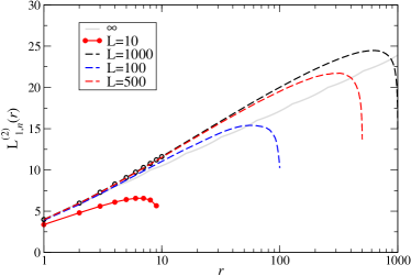
We see in Figure 7(a) that, similar to the complete binary trees considered in the section II, the leaf-to-leaf distances increase with until they reach a maximal value. Unlike the complete tree in Figure 2(a), they start to decrease rapidly beyond this point. We also see that for such small trees, we are still far from the infinite complete tree result of Equation (9). Finally, we also see that when we choose random binary trees from the possible such trees at that the average leaf-to-leaf distances for each is still distinguishably different from an exact summation of all leaf-to-leaf distances. This suggests that rare tree structures are quite important. In Figure 7(b) we nevertheless show estimates of for various . As before, the shape of the curves for large is similar to those for small . Clearly, however, the cusps in are no longer present in . Also, the values of are larger than those for for small .
VIII Conclusions
We have calculated an analytic form for the average distance between two leaves with a given separation — ordered according to the physical distance long a line — in a complete binary tree graph. This result is then generalized to a complete tree where each vertex has any finite number of children. In addition to the mean leaf-to-leaf distance, it is found that the raw moments of the distribution of leaf-to-leaf distances have an analytic form that can be expressed in a concise way in terms of the Hurwitz-Lerch Zeta function. These findings are calculated for open trees, where the leaves form an open line, periodic trees, where the leaves form a circle, and infinite trees, which is the limit where the number of levels, , goes to infinity. Each of these results has a concise form and characteristic features due to the self-similarity of the trees. We believe that these results provide a useful insight into the structure of the regular tree graphs that are relevant for the field of tensor networks Silvi et al. (2010); Gerster et al. (2014). We also note that leaf-to-leaf distances computed here are qualitatively similar, but quantitatively different from those for random-spin chains Goldsborough and Römer (2014). This points to a subtle, yet physically relevant, difference in their Hilbert space properties.
Acknowledgements.
We thank M. Bates, A. Czumaj and G. Rowlands for discussions. We would like to thank the EPSRC for financial support (EP/J003476/1) and provision of computing resources through the MidPlus Regional HPC Center (EP/K000128/1).Appendix A Some useful series expressions
A.1 Series used in section II.2
When the last sum in Equation (6a) is expanded, it is simply the sum of two geometric series. The first part can be simplified using
| (45) |
the second part uses the arithmetico-geometric series
| (46) |
A.2 Series used in section IV.1
References
- Sedgewick and Flajolet (2013) R. Sedgewick and P. Flajolet, An Introduction to the Analysis of Algorithms, 2nd ed. (Addison-Wesley, Westford, MA, 2013).
- Wiener (1947) H. Wiener, J. Am. Chem. Soc. 69, 17 (1947).
- Peskin and Schroeder (1995) M. E. Peskin and D. V. Schroeder, An Introduction to Quantum Field Theory (Westview Press, Boulder, CO, 1995).
- Rosen (2012) K. H. Rosen, Discrete Mathematics and its Applications, seventh ed. (McGraw Hill, New York, NY, 2012).
- Leckey et al. (2013) K. Leckey, R. Neininger, and W. Szpankowski, in Proceedings of ACM-SIAM Symposium on Discrete Algorithms (SODA) (SIAM, 2013).
- Szekely et al. (2011) L. A. Szekely, H. Wang, and T. Wu, Discrete Math. 311, 1197 (2011).
- Wang (2010) H. Wang, ICA bulletin 60, 62 (2010).
- Jacquet and Regnier (1988) P. Jacquet and M. Regnier, Normal limiting distribution for the size and the external path length of tries, Tech. Rep. RR-0827 (INRIA, 1988).
- Kirschenhofer et al. (1989) P. Kirschenhofer, H. Prodinger, and W. Szpankowski, Theor. Comput. Sci. 68, 1 (1989).
- Kirschenhofer et al. (1994) P. Kirschenhofer, H. Prodinger, and W. Szpankowski, SIAM J. Comput. 23, 598 (1994).
- Schollwöck (2011) U. Schollwöck, Ann. Phys. 326, 96 (2011).
- Goldsborough and Römer (2014) A. M. Goldsborough and R. A. Römer, Phys. Rev. B 89, 214203 (2014).
- Evenbly and Vidal (2011) G. Evenbly and G. Vidal, J. Stat. Phys. 145, 891 (2011).
- Silvi et al. (2010) P. Silvi, V. Giovannetti, S. Montangero, M. Rizzi, J. I. Cirac, and R. Fazio, Phys. Rev. A 81, 062335 (2010).
- Gerster et al. (2014) M. Gerster, P. Silvi, M. Rizzi, R. Fazio, T. Calarco, and S. Montangero, Phys. Rev. B 90, 125154 (2014).
- Note (1) This is the information needed by the holography methods used in Ref. Goldsborough and Römer (2014).
- Kanemitsu et al. (2000) S. Kanemitsu, M. Katsurada, and M. Yoshimoto, Aequationes Math. 59, 1 (2000).
- Srivastava (2012) H. Srivastava, in Essays in Mathematics and its Applications, edited by P. M. Pardalos and T. M. Rassias (Springer Berlin Heidelberg, 2012) pp. 431–461.
- Guillera and Sondow (2008) J. Guillera and J. Sondow, Ramanujan J. 16, 247 (2008).
- Wolfram Research Inc. (2012) Wolfram Research Inc., Mathematica Version 9.0, Champaign, IL (2012).
- Shi et al. (2006) Y.-Y. Shi, L.-M. Duan, and G. Vidal, Phys. Rev. A 74, 022320 (2006).
- Tagliacozzo et al. (2009) L. Tagliacozzo, G. Evenbly, and G. Vidal, Phys. Rev. B 80, 235127 (2009).
- Verstraete et al. (2006) F. Verstraete, M. M. Wolf, D. Perez-Garcia, and J. I. Cirac, Phys. Rev. Lett. 96, 220601 (2006).
- Wolf et al. (2006) M. M. Wolf, G. Ortiz, F. Verstraete, and J. I. Cirac, Phys. Rev. Lett. 97, 110403 (2006).
- Evenbly and Vidal (2009) G. Evenbly and G. Vidal, Phys. Rev. B 79, 144108 (2009).
- Note (2) We emphasize that this definition of a random trees is different from the definition of so-called Catalan tree graphs Sedgewick and Flajolet (2013), as the number of unique graphs is given by the Catalan number and does not double count the degenerate graphs as shown in the center of the case of Figure 6(b).
- Gradshteyn and Ryzhik (1994) I. S. Gradshteyn and I. M. Ryzhik, Table of Integrals, Series and Products (Academic Press, London, 1994).