Macroscopic limit of a bipartite Curie-Weiss model: a dynamical approach

Francesca Collet
Dipartimento di Matematica
Alma Mater Studiorum Universitร  di Bologna
Piazza di Porta San Donato 5; 40126 Bologna, Italy
e-mail: francesca.collet@unibo.it
Abstract

We analyze the Glauber dynamics for a bi-populated Curie-Weiss model. We obtain the limiting behavior of the empirical averages in the limit of infinitely many particles. We then characterize the phase space of the model in absence of magnetic field and we show that several phase transitions in the inter-groups interaction strength occur.

Keywords: Glauber dynamics, interacting particle systems, large deviations, McKean-Vlasov equation, reversible Markov processes, mean-field interaction, phase transition

1 Introduction

Theoretical models based on mean field interacting spin systems, although simplistic, are able to show a good qualitative description of cooperative macroscopic behavior in self-organizing systems. In the last decades, for this reason and their analytical tractability, they have also been applied to social sciences [BD01, CDPS10], finance [FB08, DPRST09], chemistry [DBABB12] and ecology [VBHM03, BDPF+14].
An interesting family within this class, which has naturally emerged in applications, is a multi-species extension of the Curie-Weiss model. The possibility of taking account for several kinds of magnetic spins is a peculiar feature, that may be relevant to capture diverse phenomena from magnetism in anisotropic materials [SD97] to socio-economic models [CG07]. In this last case, for instance, the possibility of partitioning a population in classes of people sharing the same characteristics yields to a more realistic modeling. In this respect, it is worth to mention a series of papers [CGM08, GBC09], where this kind of interacting particle systems and techniques coming from statistical mechanics are used not only to describe problems concerning cultural coexistence, immigration and integration in societies, but also to make predictions at the population level. This framework has been tested against experimental data with an overall good agreement [BCSV14].
In this paper, the system under consideration consists of a two-population generalization of the classical mean field Ising model. Thus, on the complete graph two types of spins are present, with an interaction which is homogeneous among sites belonging to the same group, whereas it assumes a different value between sites of distinct populations. To have more intuition it may be helpful to think of the model as an interacting mixture of two Curie-Weiss models.
In the equilibrium theory, the thermodynamic limit of the model has been rigorously obtained in [GC08], where also some preliminary results concerning the phase diagram are given. Under mild assumptions on the interaction parameters and the restriction to populations of the same size, an analytic description of the latter is provided in [FU12]. A variety of phase transitions is shown.
Here, however, we examine in detail some aspects of the dynamics of the model. We start with a Glauber dynamics for the N๐‘N-particle system, where each spin may experience a flip with a rate depending on the gradient of the Hamiltonian felt by the particle. Next we show, via a large deviation approach on path space, that a propagation of chaos result holds and establish the asymptotic dynamics of the pair of group magnetizations in the infinite volume limit. This result corresponds to a law of large numbers and it allows to describe the macroscopic evolution of the system, which is deterministic. We then give the full phase diagram of the stationary solutions in absence of external fields. In comparison with the results in [FU12], we keep complete arbitrariness of the interaction parameters and, moreover, we relax the symmetry hypothesis on the relative proportion of the groups.

Although the model itself is not a novelty in literature and its static analysis is well understood, to our knowledge we provide the first attempt of dynamical description of the time evolution of such system, obtaining also some non-equilibrium properties.
The outline of the paper is as follows. In Sectionย 2 we illustrate the model and exact statements of the results are presented. Sectionย 3 is devoted to the proofs of the main theorems stated in Sectionย 2. A Conclusions section concludes the paper.

2 Model and main results

Let ๐’ฎ={โˆ’1,+1}๐’ฎ11\mathscr{S}=\{-1,+1\} and h=(hj)j=1Nโˆˆโ„Nโ„Žsuperscriptsubscriptsubscriptโ„Ž๐‘—๐‘—1๐‘superscriptโ„๐‘h=(h_{j})_{j=1}^{N}\in\mathbb{R}^{N} be a sequence of real numbers. Given a configuration ฯƒ=(ฯƒj)j=1Nโˆˆ๐’ฎN๐œŽsuperscriptsubscriptsubscript๐œŽ๐‘—๐‘—1๐‘superscript๐’ฎ๐‘\sigma=(\sigma_{j})_{j=1}^{N}\in\mathscr{S}^{N} of a N๐‘N-spin system and a realization of the magnetic field hโ„Žh, we can define the Hamiltonian HNโ€‹(ฯƒ):๐’ฎNโŸถโ„:subscript๐ป๐‘๐œŽโŸถsuperscript๐’ฎ๐‘โ„H_{N}(\sigma):\mathscr{S}^{N}\longrightarrow\mathbb{R} as

HNโ€‹(ฯƒ)=โˆ’12โ€‹Nโ€‹โˆ‘j,k=1NJjโ€‹kโ€‹ฯƒjโ€‹ฯƒkโˆ’โˆ‘j=1Nhjโ€‹ฯƒj,subscript๐ป๐‘๐œŽ12๐‘superscriptsubscript๐‘—๐‘˜1๐‘subscript๐ฝ๐‘—๐‘˜subscript๐œŽ๐‘—subscript๐œŽ๐‘˜superscriptsubscript๐‘—1๐‘subscriptโ„Ž๐‘—subscript๐œŽ๐‘—H_{N}(\sigma)=-\frac{1}{2N}\sum_{j,k=1}^{N}J_{jk}\sigma_{j}\sigma_{k}-\sum_{j=1}^{N}h_{j}\sigma_{j}\,, (1)

where ฯƒjsubscript๐œŽ๐‘—\sigma_{j} is the spin value at site j๐‘—j and hjsubscriptโ„Ž๐‘—h_{j} the local magnetic field associated with the same site. Let Jjโ€‹ksubscript๐ฝ๐‘—๐‘˜J_{jk}, real parameter, represent the strength of the interaction between sites j๐‘—j and k๐‘˜k. Without loss of generality, we restrict to the case of symmetric matrices ๐•=(Jjโ€‹k)1โ‰คj,kโ‰คN๐•subscriptsubscript๐ฝ๐‘—๐‘˜formulae-sequence1๐‘—๐‘˜๐‘\mathbb{J}=(J_{jk})_{1\leq j,k\leq N}.
We divide the whole system of size N๐‘N into two disjoint subsystems of sizes N1subscript๐‘1N_{1} and N2subscript๐‘2N_{2} respectively. Let I1subscript๐ผ1I_{1} (resp. I2subscript๐ผ2I_{2}) be the set of sites belonging to the first (resp. second) subsystem. We have |I1|=N1subscript๐ผ1subscript๐‘1|I_{1}|=N_{1} and |I2|=N2subscript๐ผ2subscript๐‘2|I_{2}|=N_{2}, with N1+N2=Nsubscript๐‘1subscript๐‘2๐‘N_{1}+N_{2}=N. To fix notation, let 1,2,โ€ฆ,N112โ€ฆsubscript๐‘11,2,\dots,N_{1} be the indeces corresponding to particles in population I1subscript๐ผ1I_{1} and N1+1,N1+2,โ€ฆ,Nsubscript๐‘11subscript๐‘12โ€ฆ๐‘N_{1}+1,N_{1}+2,\dots,N those of particles in population I2subscript๐ผ2I_{2}, so that

Populationย I1Populationย I2ฯƒ=(ฯƒ1,ฯƒ2,โ€ฆ,ฯƒN1ฯƒN1+1,ฯƒN1+2,โ€ฆ,ฯƒN)\begin{array}[]{rc|c}&\mbox{\scriptsize Population $I_{1}$}&\mbox{\scriptsize Population $I_{2}$}\\ \sigma=&(\sigma_{1},\sigma_{2},\dots,\sigma_{N_{1}}&\sigma_{N_{1}+1},\sigma_{N_{1}+2},\dots,\sigma_{N})\end{array}

Given two spins ฯƒjsubscript๐œŽ๐‘—\sigma_{j} and ฯƒksubscript๐œŽ๐‘˜\sigma_{k}, their mutual interaction Jjโ€‹ksubscript๐ฝ๐‘—๐‘˜J_{jk} depends on the subsystems they belong to, as specified by the following matrix

๐•=(๐•11๐•12๐•21๐•22)๐•subscript๐•11missing-subexpressionsubscript๐•12missing-subexpressionmissing-subexpressionmissing-subexpressionmissing-subexpressionmissing-subexpressionmissing-subexpressionmissing-subexpressionmissing-subexpressionmissing-subexpressionsubscript๐•21missing-subexpressionsubscript๐•22missing-subexpressionmissing-subexpressionmissing-subexpressionmissing-subexpression\mathbb{J}=\begin{array}[]{rccc}\left(\begin{array}[]{c|ccc}\begin{smallmatrix}\mathbb{J}_{11}\end{smallmatrix}&&\begin{smallmatrix}\mathbb{J}_{12}\end{smallmatrix}\\ \hline\cr&&&\\ \begin{smallmatrix}\mathbb{J}_{21}\end{smallmatrix}&&\begin{smallmatrix}\mathbb{J}_{22}\end{smallmatrix}&\\ &&&\end{array}\right)\end{array}

where ๐•jโ€‹jsubscript๐•๐‘—๐‘—\mathbb{J}_{jj} is a Njร—Njsubscript๐‘๐‘—subscript๐‘๐‘—N_{j}\times N_{j} square block comprised by constant elements Jjโ€‹jsubscript๐ฝ๐‘—๐‘—J_{jj} tuning the interaction within sites of the same subsystem and ๐•jโ€‹k=๐•kโ€‹jโŠคsubscript๐•๐‘—๐‘˜subscriptsuperscript๐•top๐‘˜๐‘—\mathbb{J}_{jk}=\mathbb{J}^{\top}_{kj} is a Njร—Nksubscript๐‘๐‘—subscript๐‘๐‘˜N_{j}\times N_{k} rectangular block with constant entries Jjโ€‹ksubscript๐ฝ๐‘—๐‘˜J_{jk} controlling the interaction of spins located in different subystems. We assume J11subscript๐ฝ11J_{11} and J22subscript๐ฝ22J_{22} positive; while, J12subscript๐ฝ12J_{12} can be either positive or negative allowing both ferromagnetic and antiferromagnetic interactions.
Analogously, the field hjsubscriptโ„Ž๐‘—h_{j} can take only the two values h1subscriptโ„Ž1h_{1} or h2subscriptโ„Ž2h_{2}, depending on the subset containing ฯƒjsubscript๐œŽ๐‘—\sigma_{j}, according to the vector

h=(h1โ‹ฎh1h2โ‹ฎh2)โ€‹}N1}N2โ„Žsubscriptโ„Ž1โ‹ฎsubscriptโ„Ž1missing-subexpressionsubscriptโ„Ž2โ‹ฎsubscriptโ„Ž2casesmissing-subexpressionmissing-subexpressionsubscript๐‘1casesmissing-subexpressionmissing-subexpressionsubscript๐‘2h=\left(\begin{array}[]{c}h_{1}\\ \vdots\\ h_{1}\\ \hline\cr h_{2}\\ \vdots\\ h_{2}\end{array}\right)\begin{array}[]{ll}\left.\begin{array}[]{l}\\ \phantom{\vdots}\\ \\ \end{array}\right\}&N_{1}\\ \left.\begin{array}[]{l}\\ \phantom{\vdots}\\ \\ \end{array}\right\}&N_{2}\end{array}

We introduce the magnetization of a subset S๐‘†S as

m|S|โ€‹(ฯƒ)=1|S|โ€‹โˆ‘jโˆˆSฯƒj.subscript๐‘š๐‘†๐œŽ1๐‘†subscript๐‘—๐‘†subscript๐œŽ๐‘—m_{|S|}(\sigma)=\frac{1}{|S|}\sum_{j\in S}\sigma_{j}\,.

Moreover, we denote by ๐ฆNโ€‹(ฯƒ)=(mN1โ€‹(ฯƒ),mN2โ€‹(ฯƒ))subscript๐ฆ๐‘๐œŽsubscript๐‘šsubscript๐‘1๐œŽsubscript๐‘šsubscript๐‘2๐œŽ\mathbf{m}_{N}(\sigma)=\left(m_{N_{1}}(\sigma),m_{N_{2}}(\sigma)\right) the vector whose entries are the magnetizations of population I1subscript๐ผ1I_{1} and I2subscript๐ผ2I_{2}, respectively. By defining ฮฑ:=N1Nassign๐›ผsubscript๐‘1๐‘\alpha:=\frac{N_{1}}{N} the proportion of sites belonging to the first group, we can immediately rewrite the Hamiltonian (1) as

HNโ€‹(ฯƒ)=โˆ’N2โ€‹[ฮฑ2โ€‹J11โ€‹(mN1โ€‹(ฯƒ))2+2โ€‹ฮฑโ€‹(1โˆ’ฮฑ)โ€‹J12โ€‹mN1โ€‹(ฯƒ)โ€‹mN2โ€‹(ฯƒ)+(1โˆ’ฮฑ)2โ€‹J22โ€‹(mN2โ€‹(ฯƒ))2]โˆ’Nโ€‹ฮฑโ€‹h1โ€‹mN1โ€‹(ฯƒ)โˆ’Nโ€‹(1โˆ’ฮฑ)โ€‹h2โ€‹mN2โ€‹(ฯƒ).subscript๐ป๐‘๐œŽ๐‘2delimited-[]superscript๐›ผ2subscript๐ฝ11superscriptsubscript๐‘šsubscript๐‘1๐œŽ22๐›ผ1๐›ผsubscript๐ฝ12subscript๐‘šsubscript๐‘1๐œŽsubscript๐‘šsubscript๐‘2๐œŽsuperscript1๐›ผ2subscript๐ฝ22superscriptsubscript๐‘šsubscript๐‘2๐œŽ2๐‘๐›ผsubscriptโ„Ž1subscript๐‘šsubscript๐‘1๐œŽ๐‘1๐›ผsubscriptโ„Ž2subscript๐‘šsubscript๐‘2๐œŽH_{N}(\sigma)=-\frac{N}{2}\left[\alpha^{2}J_{11}\left(m_{N_{1}}(\sigma)\right)^{2}+2\alpha(1-\alpha)J_{12}m_{N_{1}}(\sigma)m_{N_{2}}(\sigma)+(1-\alpha)^{2}J_{22}\left(m_{N_{2}}(\sigma)\right)^{2}\right]\\ -N\alpha h_{1}m_{N_{1}}(\sigma)-N(1-\alpha)h_{2}m_{N_{2}}(\sigma)\,. (2)

Let us define the dynamics we consider. The stochastic process (ฯƒโ€‹(t))tโ‰ฅ0subscript๐œŽ๐‘ก๐‘ก0(\sigma(t))_{t\geq 0} is described as follows. Let ฯƒisuperscript๐œŽ๐‘–\sigma^{i} denote the configuration obtained from ฯƒ๐œŽ\sigma by flipping the i๐‘–i-th spin. The spins will be assumed to evolve with Glauber one spin-flip dynamics: at any time t๐‘กt, the system may experience a transition

ฯƒโŸถฯƒiย at rateย {eโˆ’ฯƒiโ€‹[R1โ€‹(๐ฆNโ€‹(ฯƒ))+h1],ย ifย โ€‹iโˆˆI1eโˆ’ฯƒiโ€‹[R2โ€‹(๐ฆNโ€‹(ฯƒ))+h2],ย ifย โ€‹iโˆˆI2,โŸถ๐œŽsuperscript๐œŽ๐‘–ย at rateย casessuperscript๐‘’subscript๐œŽ๐‘–delimited-[]subscript๐‘…1subscript๐ฆ๐‘๐œŽsubscriptโ„Ž1ย ifย ๐‘–subscript๐ผ1superscript๐‘’subscript๐œŽ๐‘–delimited-[]subscript๐‘…2subscript๐ฆ๐‘๐œŽsubscriptโ„Ž2ย ifย ๐‘–subscript๐ผ2\sigma\longrightarrow\sigma^{i}\quad\mbox{ at rate }\quad\left\{\begin{array}[]{ll}e^{-\sigma_{i}\left[R_{1}\left(\mathbf{m}_{N}(\sigma)\right)+h_{1}\right]},&\mbox{ if }i\in I_{1}\\ e^{-\sigma_{i}\left[R_{2}\left(\mathbf{m}_{N}(\sigma)\right)+h_{2}\right]},&\mbox{ if }i\in I_{2}\,,\end{array}\right.

where

R1โ€‹(๐ฑ)=ฮฑโ€‹J11โ€‹x1+(1โˆ’ฮฑ)โ€‹J12โ€‹x2ย andย R2โ€‹(๐ฑ)=ฮฑโ€‹J12โ€‹x1+(1โˆ’ฮฑ)โ€‹J22โ€‹x2.formulae-sequencesubscript๐‘…1๐ฑ๐›ผsubscript๐ฝ11subscript๐‘ฅ11๐›ผsubscript๐ฝ12subscript๐‘ฅ2ย andย subscript๐‘…2๐ฑ๐›ผsubscript๐ฝ12subscript๐‘ฅ11๐›ผsubscript๐ฝ22subscript๐‘ฅ2R_{1}\left(\mathbf{x}\right)=\alpha J_{11}x_{1}+(1-\alpha)J_{12}x_{2}\quad\mbox{ and }\quad R_{2}\left(\mathbf{x}\right)=\alpha J_{12}x_{1}+(1-\alpha)J_{22}x_{2}\,. (3)

Not to clutter our notation, we omit subscripts indicating the dependence of functions Risubscript๐‘…๐‘–R_{i}โ€™s (i=1,2๐‘–12i=1,2) on ฮฑ๐›ผ\alpha and ๐•๐•\mathbb{J}.

Formally, we are considering a continuous time Markov chain on ๐’ฎNsuperscript๐’ฎ๐‘\mathscr{S}^{N}, with infinitesimal generator LNsubscript๐ฟ๐‘L_{N} acting on functions f:๐’ฎNโŸถโ„:๐‘“โŸถsuperscript๐’ฎ๐‘โ„f:\mathscr{S}^{N}\longrightarrow\mathbb{R} as follows:

LNโ€‹fโ€‹(ฯƒ)=โˆ‘jโˆˆI1eโˆ’ฯƒjโ€‹[R1โ€‹(๐ฆNโ€‹(ฯƒ))+h1]โ€‹โˆ‡jฯƒfโ€‹(ฯƒ)+โˆ‘jโˆˆI2eโˆ’ฯƒjโ€‹[R2โ€‹(๐ฆNโ€‹(ฯƒ))+h2]โ€‹โˆ‡jฯƒfโ€‹(ฯƒ),subscript๐ฟ๐‘๐‘“๐œŽsubscript๐‘—subscript๐ผ1superscript๐‘’subscript๐œŽ๐‘—delimited-[]subscript๐‘…1subscript๐ฆ๐‘๐œŽsubscriptโ„Ž1subscriptsuperscriptโˆ‡๐œŽ๐‘—๐‘“๐œŽsubscript๐‘—subscript๐ผ2superscript๐‘’subscript๐œŽ๐‘—delimited-[]subscript๐‘…2subscript๐ฆ๐‘๐œŽsubscriptโ„Ž2subscriptsuperscriptโˆ‡๐œŽ๐‘—๐‘“๐œŽL_{N}f(\sigma)=\sum_{j\in I_{1}}e^{-\sigma_{j}\left[R_{1}\left(\mathbf{m}_{N}(\sigma)\right)+h_{1}\right]}\nabla^{\sigma}_{j}f(\sigma)+\sum_{j\in I_{2}}e^{-\sigma_{j}\left[R_{2}\left(\mathbf{m}_{N}(\sigma)\right)+h_{2}\right]}\nabla^{\sigma}_{j}f(\sigma), (4)

where โˆ‡jฯƒfโ€‹(ฯƒ)=fโ€‹(ฯƒj)โˆ’fโ€‹(ฯƒ)subscriptsuperscriptโˆ‡๐œŽ๐‘—๐‘“๐œŽ๐‘“superscript๐œŽ๐‘—๐‘“๐œŽ\nabla^{\sigma}_{j}f(\sigma)=f(\sigma^{j})-f(\sigma).

Remark 2.1.

The dynamics (4) is reversible with respect to the stationary distribution

ฮผNโ€‹(ฯƒ)=expโก[โˆ’HNโ€‹(ฯƒ)]ZN,subscript๐œ‡๐‘๐œŽsubscript๐ป๐‘๐œŽsubscript๐‘๐‘\mu_{N}(\sigma)=\frac{\exp[-H_{N}(\sigma)]}{Z_{N}}\,, (5)

with ZNsubscript๐‘๐‘Z_{N} normalizing factor depending on ฮฑ๐›ผ\alpha, ๐•๐•\mathbb{J} and hโ„Žh.

For simplicity, the initial condition ฯƒโ€‹(0)๐œŽ0\sigma(0) is assumed to have product distribution ฮปโŠ—Nsuperscript๐œ†tensor-productabsent๐‘\lambda^{\otimes N}, with ฮป๐œ†\lambda probability measure on ๐’ฎ๐’ฎ\mathscr{S}. The quantity (ฯƒjโ€‹(t))tโˆˆ[0,T]subscriptsubscript๐œŽ๐‘—๐‘ก๐‘ก0๐‘‡(\sigma_{j}(t))_{t\in[0,T]} represents the time evolution on [0,T]0๐‘‡[0,T] of j๐‘—j-th spin value. The space of all these paths is ๐’Ÿโ€‹[0,T]๐’Ÿ0๐‘‡\mathscr{D}[0,T], which is the space of the right-continuous, piecewise-constant functions from [0,T]0๐‘‡[0,T] to ๐’ฎ๐’ฎ\mathscr{S}. We endow ๐’Ÿโ€‹[0,T]๐’Ÿ0๐‘‡\mathscr{D}[0,T] with the Skorohod topology, which provides a metric and a Borel ฯƒ๐œŽ\sigma-field (seeย [EK86]).

Result I: Infinite Volume Dynamics.

We now derive the dynamics of the process (4), in the limit as NโŸถ+โˆžโŸถ๐‘N\longrightarrow+\infty, in a fixed time interval [0,T]0๐‘‡[0,T], via a large deviations approach.

Remark 2.2.

Notice that, since N1=ฮฑโ€‹Nsubscript๐‘1๐›ผ๐‘N_{1}=\alpha N and N2=(1โˆ’ฮฑ)โ€‹Nsubscript๐‘21๐›ผ๐‘N_{2}=(1-\alpha)N, in the limit as NโŸถ+โˆžโŸถ๐‘N\longrightarrow+\infty, N1subscript๐‘1N_{1} and N2subscript๐‘2N_{2} grow to infinity with the same speed as N๐‘N.

Let ฯƒโ€‹[0,T]โˆˆ(๐’Ÿโ€‹[0,T])N๐œŽ0๐‘‡superscript๐’Ÿ0๐‘‡๐‘\sigma[0,T]\in(\mathscr{D}[0,T])^{N} denote a path of the system in the time interval [0,T]0๐‘‡[0,T], with T๐‘‡T positive and fixed. If f:๐’ฎโŸถโ„:๐‘“โŸถ๐’ฎโ„f:\mathscr{S}\longrightarrow\mathbb{R}, we are interested in the asymptotic (as NโŸถ+โˆžโŸถ๐‘N\longrightarrow+\infty) behavior of the pair of empirical averages

(โˆซfโ€‹๐‘‘ฯ1โ€‹(t),โˆซfโ€‹๐‘‘ฯ2โ€‹(t)):=(1N1โ€‹โˆ‘jโˆˆI1fโ€‹(ฯƒjโ€‹(t)),1N2โ€‹โˆ‘jโˆˆI2fโ€‹(ฯƒjโ€‹(t))),assign๐‘“differential-dsubscript๐œŒ1๐‘ก๐‘“differential-dsubscript๐œŒ2๐‘ก1subscript๐‘1subscript๐‘—subscript๐ผ1๐‘“subscript๐œŽ๐‘—๐‘ก1subscript๐‘2subscript๐‘—subscript๐ผ2๐‘“subscript๐œŽ๐‘—๐‘ก\left(\int fd\rho_{1}(t),\int fd\rho_{2}(t)\right):=\left(\frac{1}{N_{1}}\sum_{j\in I_{1}}f(\sigma_{j}(t)),\frac{1}{N_{2}}\sum_{j\in I_{2}}f(\sigma_{j}(t))\right)\,,

where ๐†Nโ€‹(t):=(ฯ1โ€‹(t),ฯ2โ€‹(t))tโˆˆ[0,T]assignsubscript๐†๐‘๐‘กsubscriptsubscript๐œŒ1๐‘กsubscript๐œŒ2๐‘ก๐‘ก0๐‘‡\boldsymbol{\rho}_{N}(t):=(\rho_{1}(t),\rho_{2}(t))_{t\in[0,T]} is the flow of the pair of empirical measures

(ฯ1โ€‹(t),ฯ2โ€‹(t))=(1N1โ€‹โˆ‘jโˆˆI1ฮดฯƒjโ€‹(t),1N2โ€‹โˆ‘jโˆˆI2ฮดฯƒjโ€‹(t)).subscript๐œŒ1๐‘กsubscript๐œŒ2๐‘ก1subscript๐‘1subscript๐‘—subscript๐ผ1subscript๐›ฟsubscript๐œŽ๐‘—๐‘ก1subscript๐‘2subscript๐‘—subscript๐ผ2subscript๐›ฟsubscript๐œŽ๐‘—๐‘ก(\rho_{1}(t),\rho_{2}(t))=\left(\frac{1}{N_{1}}\sum_{j\in I_{1}}\delta_{\sigma_{j}(t)},\frac{1}{N_{2}}\sum_{j\in I_{2}}\delta_{\sigma_{j}(t)}\right)\,.

We may think of ๐†Nsubscript๐†๐‘\boldsymbol{\rho}_{N} as a random element of โ„ณ1โ€‹(๐’Ÿโ€‹[0,T])ร—โ„ณ1โ€‹(๐’Ÿโ€‹[0,T])subscriptโ„ณ1๐’Ÿ0๐‘‡subscriptโ„ณ1๐’Ÿ0๐‘‡\mathscr{M}_{1}(\mathscr{D}[0,T])\times\mathscr{M}_{1}(\mathscr{D}[0,T]), where โ„ณ1โ€‹(๐’Ÿโ€‹[0,T])subscriptโ„ณ1๐’Ÿ0๐‘‡\mathscr{M}_{1}(\mathscr{D}[0,T]) is the space of probability measures on ๐’Ÿโ€‹[0,T]๐’Ÿ0๐‘‡\mathscr{D}[0,T] endowed with the weak convergence topology.
First of all, we want to determine the weak limit of ๐†Nsubscript๐†๐‘\boldsymbol{\rho}_{N} in โ„ณ1โ€‹(๐’Ÿโ€‹[0,T])ร—โ„ณ1โ€‹(๐’Ÿโ€‹[0,T])subscriptโ„ณ1๐’Ÿ0๐‘‡subscriptโ„ณ1๐’Ÿ0๐‘‡\mathscr{M}_{1}(\mathscr{D}[0,T])\times\mathscr{M}_{1}(\mathscr{D}[0,T]) as N๐‘N grows to infinity. It corresponds to a law of large numbers with the limit being a deterministic measure. Being an element of โ„ณ1โ€‹(๐’Ÿโ€‹[0,T])ร—โ„ณ1โ€‹(๐’Ÿโ€‹[0,T])subscriptโ„ณ1๐’Ÿ0๐‘‡subscriptโ„ณ1๐’Ÿ0๐‘‡\mathscr{M}_{1}(\mathscr{D}[0,T])\times\mathscr{M}_{1}(\mathscr{D}[0,T]), such a limit can be viewed as a stochastic process, which describes the dynamics of the system in the infinite volume limit.
The result we actually prove is a large deviation principle for the distribution of ๐†Nsubscript๐†๐‘\boldsymbol{\rho}_{N}. To state it properly we need some more notation.

Consider ๐‘ธ=(Q1,Q2)โˆˆโ„ณ1โ€‹(๐’Ÿโ€‹[0,T])ร—โ„ณ1โ€‹(๐’Ÿโ€‹[0,T])๐‘ธsubscript๐‘„1subscript๐‘„2subscriptโ„ณ1๐’Ÿ0๐‘‡subscriptโ„ณ1๐’Ÿ0๐‘‡\boldsymbol{Q}=(Q_{1},Q_{2})\in\mathscr{M}_{1}(\mathscr{D}[0,T])\times\mathscr{M}_{1}(\mathscr{D}[0,T]), if ๐‘ธโ€‹(t)=(Q1โ€‹(t),Q2โ€‹(t))๐‘ธ๐‘กsubscript๐‘„1๐‘กsubscript๐‘„2๐‘ก\boldsymbol{Q}(t)=(Q_{1}(t),Q_{2}(t)) indicates the marginal distribution of ๐‘ธ๐‘ธ\boldsymbol{Q} at time t๐‘กt, then we denote

๐ฆ๐‘ธโ€‹(t)โ€‹(ฮท)=(โˆซ๐’ฎฮทโ€‹Q1โ€‹(t;dโ€‹ฮท),โˆซ๐’ฎฮทโ€‹Q2โ€‹(t;dโ€‹ฮท)).subscript๐ฆ๐‘ธ๐‘ก๐œ‚subscript๐’ฎ๐œ‚subscript๐‘„1๐‘ก๐‘‘๐œ‚subscript๐’ฎ๐œ‚subscript๐‘„2๐‘ก๐‘‘๐œ‚\mathbf{m}_{\boldsymbol{Q}(t)}(\eta)=\left(\int_{\mathscr{S}}\eta\,Q_{1}(t;d\eta),\int_{\mathscr{S}}\eta\,Q_{2}(t;d\eta)\right)\,.

We will often use this notation in the rest of the paper. Besides, for a given path ฮทโ€‹[0,T]โˆˆ๐’Ÿโ€‹[0,T]๐œ‚0๐‘‡๐’Ÿ0๐‘‡\eta[0,T]\in\mathscr{D}[0,T] (observe that it is a single spin trajectory), we define

Fโ€‹(๐‘ธ):=ฮฑโ€‹F1โ€‹(Q1)+(1โˆ’ฮฑ)โ€‹F2โ€‹(Q2)assign๐น๐‘ธ๐›ผsubscript๐น1subscript๐‘„11๐›ผsubscript๐น2subscript๐‘„2F(\boldsymbol{Q}):=\alpha F_{1}(Q_{1})+(1-\alpha)F_{2}(Q_{2}) (6)

with

F1(Q1):=โˆซ{โˆซ0T(1โˆ’eโˆ’ฮทโ€‹(t)โ€‹[R1โ€‹(๐ฆ๐‘ธโ€‹(t)โ€‹(ฮท))+h1])dt+ฮทโ€‹(T)2[R1(๐ฆ๐‘ธโ€‹(T)(ฮท))+h1]โˆ’ฮทโ€‹(0)2[R1(๐ฆ๐‘ธโ€‹(0)(ฮท))+h1]}dQ1assignsubscript๐น1subscript๐‘„1superscriptsubscript0๐‘‡1superscript๐‘’๐œ‚๐‘กdelimited-[]subscript๐‘…1subscript๐ฆ๐‘ธ๐‘ก๐œ‚subscriptโ„Ž1๐‘‘๐‘ก๐œ‚๐‘‡2delimited-[]subscript๐‘…1subscript๐ฆ๐‘ธ๐‘‡๐œ‚subscriptโ„Ž1๐œ‚02delimited-[]subscript๐‘…1subscript๐ฆ๐‘ธ0๐œ‚subscriptโ„Ž1๐‘‘subscript๐‘„1F_{1}(Q_{1}):=\int\bigg{\{}\int_{0}^{T}\left(1-e^{-\eta(t)\left[R_{1}\left(\mathbf{m}_{\boldsymbol{Q}(t)}(\eta)\right)+h_{1}\right]}\right)dt+\frac{\eta(T)}{2}\left[R_{1}\left(\mathbf{m}_{\boldsymbol{Q}(T)}(\eta)\right)+h_{1}\right]\\ -\frac{\eta(0)}{2}\left[R_{1}\left(\mathbf{m}_{\boldsymbol{Q}(0)}(\eta)\right)+h_{1}\right]\bigg{\}}dQ_{1} (7a)
and
F2(Q2):=โˆซ{โˆซ0T(1โˆ’eโˆ’ฮทโ€‹(t)โ€‹[R2โ€‹(๐ฆ๐‘ธโ€‹(t)โ€‹(ฮท))+h2])dt+ฮทโ€‹(T)2[R2(๐ฆ๐‘ธโ€‹(T)(ฮท))+h2]โˆ’ฮทโ€‹(0)2[R2(๐ฆ๐‘ธโ€‹(0)(ฮท))+h2]}dQ2.assignsubscript๐น2subscript๐‘„2superscriptsubscript0๐‘‡1superscript๐‘’๐œ‚๐‘กdelimited-[]subscript๐‘…2subscript๐ฆ๐‘ธ๐‘ก๐œ‚subscriptโ„Ž2๐‘‘๐‘ก๐œ‚๐‘‡2delimited-[]subscript๐‘…2subscript๐ฆ๐‘ธ๐‘‡๐œ‚subscriptโ„Ž2๐œ‚02delimited-[]subscript๐‘…2subscript๐ฆ๐‘ธ0๐œ‚subscriptโ„Ž2๐‘‘subscript๐‘„2F_{2}(Q_{2}):=\int\bigg{\{}\int_{0}^{T}\left(1-e^{-\eta(t)\left[R_{2}\left(\mathbf{m}_{\boldsymbol{Q}(t)}(\eta)\right)+h_{2}\right]}\right)dt+\frac{\eta(T)}{2}\left[R_{2}\left(\mathbf{m}_{\boldsymbol{Q}(T)}(\eta)\right)+h_{2}\right]\\ -\frac{\eta(0)}{2}\left[R_{2}\left(\mathbf{m}_{\boldsymbol{Q}(0)}(\eta)\right)+h_{2}\right]\bigg{\}}dQ_{2}\,. (7b)

If PNsubscript๐‘ƒ๐‘P_{N} is the law of ฯƒโ€‹[0,T]โˆˆ(๐’Ÿโ€‹[0,T])N๐œŽ0๐‘‡superscript๐’Ÿ0๐‘‡๐‘\sigma[0,T]\in(\mathscr{D}[0,T])^{N}, the process with infinitesimal generator (4) and initial distribution ฮปโŠ—Nsuperscript๐œ†tensor-productabsent๐‘\lambda^{\otimes N}, then let ๐’ซNsubscript๐’ซ๐‘\mathcal{P}_{N} be the law of ๐†Nโ€‹(ฯƒโ€‹[0,T])subscript๐†๐‘๐œŽ0๐‘‡\boldsymbol{\rho}_{N}(\sigma[0,T]) under PNsubscript๐‘ƒ๐‘P_{N}, i.e. ๐’ซNโ€‹(โ‹…):=PNโ€‹{๐†Nโˆˆโ‹…}assignsubscript๐’ซ๐‘โ‹…subscript๐‘ƒ๐‘subscript๐†๐‘โ‹…\mathcal{P}_{N}(\cdot):=P_{N}\{\boldsymbol{\rho}_{N}\in\cdot\}.
A special case is when all the sites are independent from each other (absence of interaction) and the spin sign change with constant rate equal to 111. We denote by W๐‘ŠW the marginal law on ๐’Ÿโ€‹[0,T]๐’Ÿ0๐‘‡\mathscr{D}[0,T] of this process.
In what follows, for every ฯ€1,ฯ€2โˆˆโ„ณ1โ€‹(๐’Ÿโ€‹[0,T])subscript๐œ‹1subscript๐œ‹2subscriptโ„ณ1๐’Ÿ0๐‘‡\pi_{1},\pi_{2}\in\mathscr{M}_{1}(\mathscr{D}[0,T]), the quantity

Hโ€‹(ฯ€1|ฯ€2):={โˆซ๐‘‘ฯ€1โ€‹logโกdโ€‹ฯ€1dโ€‹ฯ€2ifฯ€1โ‰ชฯ€2andlogโกdโ€‹ฯ€1dโ€‹ฯ€2โˆˆL1โ€‹(ฯ€1)+โˆžotherwiseassign๐ปconditionalsubscript๐œ‹1subscript๐œ‹2casesdifferential-dsubscript๐œ‹1๐‘‘subscript๐œ‹1๐‘‘subscript๐œ‹2formulae-sequencemuch-less-thanifsubscript๐œ‹1subscript๐œ‹2and๐‘‘subscript๐œ‹1๐‘‘subscript๐œ‹2superscript๐ฟ1subscript๐œ‹1otherwiseH(\pi_{1}|\pi_{2}):=\left\{\begin{array}[]{ll}\int d\pi_{1}\log\frac{d\pi_{1}}{d\pi_{2}}&\mbox{if}\quad\pi_{1}\ll\pi_{2}\quad\mbox{and}\quad\log\frac{d\pi_{1}}{d\pi_{2}}\in L^{1}(\pi_{1})\\ +\infty&\mbox{otherwise}\end{array}\right.

will represent the relative entropy between ฯ€1subscript๐œ‹1\pi_{1} and ฯ€2subscript๐œ‹2\pi_{2}.

Theorem 2.1.

The laws {๐’ซN}Nโ‰ฅ1subscriptsubscript๐’ซ๐‘๐‘1\{\mathcal{P}_{N}\}_{N\geq 1} of ๐›’Nsubscript๐›’๐‘\boldsymbol{\rho}_{N} obey a Large Deviation Principle with good rate function

โ„โ€‹(๐‘ธ):=ฮฑโ€‹Hโ€‹(Q1|W)+(1โˆ’ฮฑ)โ€‹Hโ€‹(Q2|W)โˆ’Fโ€‹(๐‘ธ).assignโ„๐‘ธ๐›ผ๐ปconditionalsubscript๐‘„1๐‘Š1๐›ผ๐ปconditionalsubscript๐‘„2๐‘Š๐น๐‘ธ\mathcal{I}(\boldsymbol{Q}):=\alpha H(Q_{1}|W)+(1-\alpha)H(Q_{2}|W)-F(\boldsymbol{Q})\,. (8)

The proof of Theorem 2.1, as well as of the other results stated in this section, is postponed to Section 3.
We recall that the above statement means that, for every C,OโŠ†โ„ณ1โ€‹(๐’Ÿโ€‹[0,T])ร—โ„ณ1โ€‹(๐’Ÿโ€‹[0,T])๐ถ๐‘‚subscriptโ„ณ1๐’Ÿ0๐‘‡subscriptโ„ณ1๐’Ÿ0๐‘‡C,O\subseteq\mathscr{M}_{1}(\mathscr{D}[0,T])\times\mathscr{M}_{1}(\mathscr{D}[0,T]) respectively closed and open for the weak topology, we have

lim supNโ†’+โˆž1Nโ€‹logโก๐’ซNโ€‹(C)โ‰คโˆ’inf๐‘ธโˆˆCโ„โ€‹(๐‘ธ)subscriptlimit-supremumโ†’๐‘1๐‘subscript๐’ซ๐‘๐ถsubscriptinfimum๐‘ธ๐ถโ„๐‘ธ\limsup_{N\to+\infty}\frac{1}{N}\log\mathcal{P}_{N}(C)\leq-\inf_{\boldsymbol{Q}\in C}\mathcal{I}(\boldsymbol{Q}) (9a)
lim infNโ†’+โˆž1Nโ€‹logโก๐’ซNโ€‹(O)โ‰ฅโˆ’inf๐‘ธโˆˆOโ„โ€‹(๐‘ธ).subscriptlimit-infimumโ†’๐‘1๐‘subscript๐’ซ๐‘๐‘‚subscriptinfimum๐‘ธ๐‘‚โ„๐‘ธ\liminf_{N\to+\infty}\frac{1}{N}\log\mathcal{P}_{N}(O)\geq-\inf_{\boldsymbol{Q}\in O}\mathcal{I}(\boldsymbol{Q})\,. (9b)

Besides, the function โ„โ€‹(โ‹…)โ„โ‹…\mathcal{I}(\cdot) is nonnegative, lower semi-continuous and the level sets {๐‘ธ:โ„โ€‹(๐‘ธ)โ‰คk}conditional-set๐‘ธโ„๐‘ธ๐‘˜\left\{\boldsymbol{Q}:\mathcal{I}(\boldsymbol{Q})\leq k\right\} are compact, for every positive k๐‘˜k. Seeย [DZ93] for more details.
The large deviation principle allows to characterize the unique limit ๐‘ธโˆ—superscript๐‘ธ\boldsymbol{Q}^{*} of the sequence {๐†N}Nโ‰ฅ1subscriptsubscript๐†๐‘๐‘1\left\{\boldsymbol{\rho}_{N}\right\}_{N\geq 1} and, in particular, makes possible to provide a Fokker-Planck equation useful to describe the time evolution of such limiting probability measure.

Theorem 2.2.

Suppose that the initial distribution of the Markov process (ฯƒโ€‹(t))tโ‰ฅ0subscript๐œŽ๐‘ก๐‘ก0(\sigma(t))_{t\geq 0} with generator (4) is such that the random variables (ฯƒjโ€‹(0))j=1Nsuperscriptsubscriptsubscript๐œŽ๐‘—0๐‘—1๐‘(\sigma_{j}(0))_{j=1}^{N} are independent and identically distributed with law ฮป๐œ†\lambda. Then the equation โ„โ€‹(๐)=0โ„๐0\mathcal{I}(\boldsymbol{Q})=0 admits a unique solution ๐โˆ—โˆˆโ„ณ1โ€‹(๐’Ÿโ€‹[0,T])ร—โ„ณ1โ€‹(๐’Ÿโ€‹[0,T])superscript๐subscriptโ„ณ1๐’Ÿ0๐‘‡subscriptโ„ณ1๐’Ÿ0๐‘‡\boldsymbol{Q}^{*}\in\mathscr{M}_{1}(\mathscr{D}[0,T])\times\mathscr{M}_{1}(\mathscr{D}[0,T]), such that its time marginal ๐ชโ€‹(t):=๐โˆ—โ€‹(t)=(q1โ€‹(t),q2โ€‹(t))โˆˆโ„ณ1โ€‹(๐’ฎ)ร—โ„ณ1โ€‹(๐’ฎ)assign๐ช๐‘กsuperscript๐๐‘กsubscript๐‘ž1๐‘กsubscript๐‘ž2๐‘กsubscriptโ„ณ1๐’ฎsubscriptโ„ณ1๐’ฎ\boldsymbol{q}(t):=\boldsymbol{Q}^{*}(t)=\left(q_{1}(t),q_{2}(t)\right)\in\mathscr{M}_{1}(\mathscr{S})\times\mathscr{M}_{1}(\mathscr{S}) have components which are weak solutions of the nonlinear McKean-Vlasov equation

โˆ‚tqiโ€‹(t)=โ„’iโ€‹qiโ€‹(t)qiโ€‹(0)=ฮป(tโˆˆ[0,T];i=1,2)subscript๐‘กsubscript๐‘ž๐‘–๐‘กsubscriptโ„’๐‘–subscript๐‘ž๐‘–๐‘กsubscript๐‘ž๐‘–0๐œ†formulae-sequence๐‘ก0๐‘‡๐‘–12\begin{array}[]{l}\partial_{t}q_{i}(t)=\mathcal{L}_{i}q_{i}(t)\\ q_{i}(0)=\lambda\end{array}\qquad(t\in[0,T];i=1,2) (10)

where

โ„’iโ€‹qiโ€‹(t;ฮท)=โˆ‡ฮท{eโˆ’ฮทโ€‹[Riโ€‹(๐ฆ๐’’โ€‹(t)โ€‹(ฮท))+hi]โ€‹qiโ€‹(t;ฮท)}.subscriptโ„’๐‘–subscript๐‘ž๐‘–๐‘ก๐œ‚superscriptโˆ‡๐œ‚superscript๐‘’๐œ‚delimited-[]subscript๐‘…๐‘–subscript๐ฆ๐’’๐‘ก๐œ‚subscriptโ„Ž๐‘–subscript๐‘ž๐‘–๐‘ก๐œ‚\mathcal{L}_{i}q_{i}(t;\eta)=\nabla^{\eta}\left\{e^{-\eta\left[R_{i}\left(\mathbf{m}_{\boldsymbol{q}(t)}(\eta)\right)+h_{i}\right]}q_{i}(t;\eta)\right\}\,.

with ฮทโˆˆ๐’ฎ๐œ‚๐’ฎ\eta\in\mathscr{S} and the Risubscript๐‘…๐‘–R_{i}โ€™s defined by (3). Moreover, with respect to a metric dโ€‹(โ‹…,โ‹…)๐‘‘โ‹…โ‹…d(\cdot,\cdot) inducing the weak topology, ๐›’NโŸถ๐โˆ—โŸถsubscript๐›’๐‘superscript๐\boldsymbol{\rho}_{N}\longrightarrow\boldsymbol{Q}^{*} in probability with exponential rate, i.e. ๐’ซNโ€‹{dโ€‹(๐›’N,๐โˆ—)>ฮต}subscript๐’ซ๐‘๐‘‘subscript๐›’๐‘superscript๐๐œ€\mathcal{P}_{N}\left\{d\left(\boldsymbol{\rho}_{N},\boldsymbol{Q}^{*}\right)>\varepsilon\right\} is exponentially small in N๐‘N, for each ฮต>0๐œ€0\varepsilon>0.

Result II: Phase Diagram.

The equation (10) describes the behavior of the system governed by generator (4) in the infinite volume limit. We are interested in the detection of the t๐‘กt-stationary solutions of this equation and in the analysis of their stability to get a full understanding of the phase diagram.
First of all, it is convenient to reformulate the McKean-Vlasov equation (10) in terms of the expectations mq1โ€‹(t)subscript๐‘šsubscript๐‘ž1๐‘กm_{q_{1}(t)} and mq2โ€‹(t)subscript๐‘šsubscript๐‘ž2๐‘กm_{q_{2}(t)} defined as follows:

mqiโ€‹(t):=โˆ‘ฮทโˆˆ๐’ฎฮทโ€‹qiโ€‹(t;ฮท)ย forย โ€‹i=1,2.formulae-sequenceassignsubscript๐‘šsubscript๐‘ž๐‘–๐‘กsubscript๐œ‚๐’ฎ๐œ‚subscript๐‘ž๐‘–๐‘ก๐œ‚ย forย ๐‘–12m_{q_{i}(t)}:=\sum_{\eta\in\mathscr{S}}\eta\,q_{i}(t;\eta)\quad\mbox{ for }i=1,2.

In the sequel, by abuse of notation we write miโ€‹(t)subscript๐‘š๐‘–๐‘กm_{i}(t) instead of mqiโ€‹(t)subscript๐‘šsubscript๐‘ž๐‘–๐‘กm_{q_{i}(t)}, for i=1,2๐‘–12i=1,2, and we denote by ๐ฆโ€‹(t)=(m1โ€‹(t),m2โ€‹(t))๐ฆ๐‘กsubscript๐‘š1๐‘กsubscript๐‘š2๐‘ก\mathbf{m}(t)=\left(m_{1}(t),m_{2}(t)\right).
To rewrite (10) in terms of the new variables m1โ€‹(t)subscript๐‘š1๐‘กm_{1}(t) and m2โ€‹(t)subscript๐‘š2๐‘กm_{2}(t), observe that

mห™1โ€‹(t)=โˆ‘ฮทโˆˆ๐’ฎฮทโ€‹qห™1โ€‹(t;ฮท)=โˆ‘ฮทโˆˆ๐’ฎฮทโ€‹โ„’1โ€‹q1โ€‹(t;ฮท).subscriptห™๐‘š1๐‘กsubscript๐œ‚๐’ฎ๐œ‚subscriptห™๐‘ž1๐‘ก๐œ‚subscript๐œ‚๐’ฎ๐œ‚subscriptโ„’1subscript๐‘ž1๐‘ก๐œ‚\dot{m}_{1}(t)=\sum_{\eta\in\mathscr{S}}\eta\,\dot{q}_{1}(t;\eta)=\sum_{\eta\in\mathscr{S}}\eta\,\mathcal{L}_{1}q_{1}(t;\eta)\,.

On the other hand, a straightforward computation yields that

โˆ‘ฮทโˆˆ๐’ฎฮทโ€‹โ„’1โ€‹q1โ€‹(t;ฮท)=2โ€‹sinhโก[R1โ€‹(๐ฆโ€‹(t))+h1]โˆ’2โ€‹m1โ€‹(t)โ€‹coshโก[R1โ€‹(๐ฆโ€‹(t))+h1],subscript๐œ‚๐’ฎ๐œ‚subscriptโ„’1subscript๐‘ž1๐‘ก๐œ‚2subscript๐‘…1๐ฆ๐‘กsubscriptโ„Ž12subscript๐‘š1๐‘กsubscript๐‘…1๐ฆ๐‘กsubscriptโ„Ž1\sum_{\eta\in\mathscr{S}}\eta\,\mathcal{L}_{1}q_{1}(t;\eta)=2\sinh\left[R_{1}\left(\mathbf{m}(t)\right)+h_{1}\right]-2m_{1}(t)\cosh\left[R_{1}\left(\mathbf{m}(t)\right)+h_{1}\right]\,,

giving

mห™1โ€‹(t)=2โ€‹sinhโก[R1โ€‹(๐ฆโ€‹(t))+h1]โˆ’2โ€‹m1โ€‹(t)โ€‹coshโก[R1โ€‹(๐ฆโ€‹(t))+h1].subscriptห™๐‘š1๐‘ก2subscript๐‘…1๐ฆ๐‘กsubscriptโ„Ž12subscript๐‘š1๐‘กsubscript๐‘…1๐ฆ๐‘กsubscriptโ„Ž1\dot{m}_{1}(t)=2\sinh\left[R_{1}\left(\mathbf{m}(t)\right)+h_{1}\right]-2m_{1}(t)\cosh\left[R_{1}\left(\mathbf{m}(t)\right)+h_{1}\right]\,.

Similarly, we can obtain an equation for m2โ€‹(t)subscript๐‘š2๐‘กm_{2}(t), so that it is proved that (10) can be rewritten as

mห™1โ€‹(t)=2โ€‹sinhโก[R1โ€‹(๐ฆโ€‹(t))+h1]โˆ’2โ€‹m1โ€‹(t)โ€‹coshโก[R1โ€‹(๐ฆโ€‹(t))+h1]mห™2โ€‹(t)=2โ€‹sinhโก[R2โ€‹(๐ฆโ€‹(t))+h2]โˆ’2โ€‹m2โ€‹(t)โ€‹coshโก[R2โ€‹(๐ฆโ€‹(t))+h2],subscriptห™๐‘š1๐‘ก2subscript๐‘…1๐ฆ๐‘กsubscriptโ„Ž12subscript๐‘š1๐‘กsubscript๐‘…1๐ฆ๐‘กsubscriptโ„Ž1subscriptห™๐‘š2๐‘ก2subscript๐‘…2๐ฆ๐‘กsubscriptโ„Ž22subscript๐‘š2๐‘กsubscript๐‘…2๐ฆ๐‘กsubscriptโ„Ž2\begin{array}[]{lcl}\dot{m}_{1}(t)&=&2\sinh\left[R_{1}\left(\mathbf{m}(t)\right)+h_{1}\right]-2m_{1}(t)\cosh\left[R_{1}\left(\mathbf{m}(t)\right)+h_{1}\right]\\ \dot{m}_{2}(t)&=&2\sinh\left[R_{2}\left(\mathbf{m}(t)\right)+h_{2}\right]-2m_{2}(t)\cosh\left[R_{2}\left(\mathbf{m}(t)\right)+h_{2}\right]\,,\end{array} (11)

with initial condition m1โ€‹(0)=m2โ€‹(0)=mฮปsubscript๐‘š10subscript๐‘š20subscript๐‘š๐œ†m_{1}(0)=m_{2}(0)=m_{\lambda}.

The following theorem is concerned with equilibria of equation (11), in the case of absence of magnetic fields. In particular, it is shown that the system undergoes several phase transitions depending on the parameters.

Theorem 2.3.

Consider the system (11) with h1=h2=0subscriptโ„Ž1subscriptโ„Ž20h_{1}=h_{2}=0 and fix ฮฑ>12๐›ผ12\alpha>\frac{1}{2}. Moreover, set

J12(c):=(1โˆ’ฮฑโ€‹J11)โ€‹(1โˆ’(1โˆ’ฮฑ)โ€‹J22)ฮฑโ€‹(1โˆ’ฮฑ).assignsuperscriptsubscript๐ฝ12๐‘1๐›ผsubscript๐ฝ1111๐›ผsubscript๐ฝ22๐›ผ1๐›ผJ_{12}^{(c)}:=\sqrt{\frac{(1-\alpha J_{11})(1-(1-\alpha)J_{22})}{\alpha(1-\alpha)}}\,.
  1. (a)

    If ฮฑโ€‹J11โ‰ค1๐›ผsubscript๐ฝ111\alpha J_{11}\leq 1 and (1โˆ’ฮฑ)โ€‹J22โ‰ค11๐›ผsubscript๐ฝ221(1-\alpha)J_{22}\leq 1, then

    1. (i)

      for |J12|โ‰คJ12(c)subscript๐ฝ12superscriptsubscript๐ฝ12๐‘|J_{12}|\leq J_{12}^{(c)} the equation (11) admits a unique equilibrium solution ๐ฆ(0)superscript๐ฆ0\mathbf{m}^{(0)}. If |J12|<J12(c)subscript๐ฝ12superscriptsubscript๐ฝ12๐‘|J_{12}|<J_{12}^{(c)} it is linearly stable, while if |J12|=J12(c)subscript๐ฝ12superscriptsubscript๐ฝ12๐‘|J_{12}|=J_{12}^{(c)} the linearized system has a neutral direction.

    2. (ii)

      for |J12|>J12(c)subscript๐ฝ12superscriptsubscript๐ฝ12๐‘|J_{12}|>J_{12}^{(c)} the point ๐ฆ(0)superscript๐ฆ0\mathbf{m}^{(0)} is still an equilibrium for (11), but it is a saddle point for the linearized system. Moreover, (11) has two linearly stable stationary solutions ยฑ๐ฆ(1)plus-or-minussuperscript๐ฆ1\pm\mathbf{m}^{(1)}.

  2. (b)

    If ฮฑโ€‹J11โ‰ค1๐›ผsubscript๐ฝ111\alpha J_{11}\leq 1 and (1โˆ’ฮฑ)โ€‹J22>11๐›ผsubscript๐ฝ221(1-\alpha)J_{22}>1 (or analogously ฮฑโ€‹J11>1๐›ผsubscript๐ฝ111\alpha J_{11}>1 and (1โˆ’ฮฑ)โ€‹J22โ‰ค11๐›ผsubscript๐ฝ221(1-\alpha)J_{22}\leq 1), then for every value of J12subscript๐ฝ12J_{12} there are three stationary solutions of (11): ๐ฆ(0)superscript๐ฆ0\mathbf{m}^{(0)}, which is a saddle point for the linearized system, and two linearly stable equilibria ยฑ๐ฆ(1)plus-or-minussuperscript๐ฆ1\pm\mathbf{m}^{(1)}.

  3. (c)

    If ฮฑโ€‹J11>1๐›ผsubscript๐ฝ111\alpha J_{11}>1 and (1โˆ’ฮฑ)โ€‹J22>11๐›ผsubscript๐ฝ221(1-\alpha)J_{22}>1, then there exists another critical value J~12(c)superscriptsubscript~๐ฝ12๐‘\widetilde{J}_{12}^{(c)}, with 0<J~12(c)<J12(c)0superscriptsubscript~๐ฝ12๐‘superscriptsubscript๐ฝ12๐‘0<\widetilde{J}_{12}^{(c)}<J_{12}^{(c)}, such that

    1. (i)

      for |J12|<J~12(c)subscript๐ฝ12superscriptsubscript~๐ฝ12๐‘|J_{12}|<\widetilde{J}_{12}^{(c)} the stationary solutions of (11) are nine: ๐ฆ(0)superscript๐ฆ0\mathbf{m}^{(0)}, which is linearly unstable; ยฑ๐ฆ(1)plus-or-minussuperscript๐ฆ1\pm\mathbf{m}^{(1)} and ยฑ๐ฆ(2)plus-or-minussuperscript๐ฆ2\pm\mathbf{m}^{(2)}, which are linearly stable; ยฑ๐ฌ(1)plus-or-minussuperscript๐ฌ1\pm\mathbf{s}^{(1)} and ยฑ๐ฌ(2)plus-or-minussuperscript๐ฌ2\pm\mathbf{s}^{(2)}, that are saddle points for the linearized system.

    2. (ii)

      for J~12(c)<|J12|<J12(c)superscriptsubscript~๐ฝ12๐‘subscript๐ฝ12superscriptsubscript๐ฝ12๐‘\widetilde{J}_{12}^{(c)}<|J_{12}|<J_{12}^{(c)} the critical points of (11) reduce to five: ๐ฆ(0)superscript๐ฆ0\mathbf{m}^{(0)}, which is still linearly unstable; ยฑ๐ฆ(1)plus-or-minussuperscript๐ฆ1\pm\mathbf{m}^{(1)}, which are linearly stable and ยฑ๐ฌ(1)plus-or-minussuperscript๐ฌ1\pm\mathbf{s}^{(1)}, that are saddle points for the linearized system.

    3. (iii)

      for |J12|โ‰ฅJ12(c)subscript๐ฝ12superscriptsubscript๐ฝ12๐‘|J_{12}|\geq J_{12}^{(c)} the equilibria of (11) become three: ๐ฆ(0)superscript๐ฆ0\mathbf{m}^{(0)} and ยฑ๐ฆ(1)plus-or-minussuperscript๐ฆ1\pm\mathbf{m}^{(1)}. The points ยฑ๐ฆ(1)plus-or-minussuperscript๐ฆ1\pm\mathbf{m}^{(1)} are linearly stable; ๐ฆ(0)superscript๐ฆ0\mathbf{m}^{(0)} is a saddle point if |J12|>J12(c)subscript๐ฝ12superscriptsubscript๐ฝ12๐‘|J_{12}|>J_{12}^{(c)}, while if |J12|=J12(c)subscript๐ฝ12superscriptsubscript๐ฝ12๐‘|J_{12}|=J_{12}^{(c)} the linearized system has a neutral direction.

In all ranges of the parameters ๐ฆ(0)=๐ŸŽsuperscript๐ฆ00\mathbf{m}^{(0)}=\boldsymbol{0}; whereas, the coordinates of the points ยฑ๐ฆ(1)plus-or-minussuperscript๐ฆ1\pm\mathbf{m}^{(1)}, ยฑ๐ฆ(2)plus-or-minussuperscript๐ฆ2\pm\mathbf{m}^{(2)}, ยฑ๐ฌ(1)plus-or-minussuperscript๐ฌ1\pm\mathbf{s}^{(1)} and ยฑ๐ฌ(2)plus-or-minussuperscript๐ฌ2\pm\mathbf{s}^{(2)} depend on ฮฑ๐›ผ\alpha and ๐•๐•\mathbb{J}.

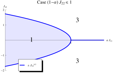
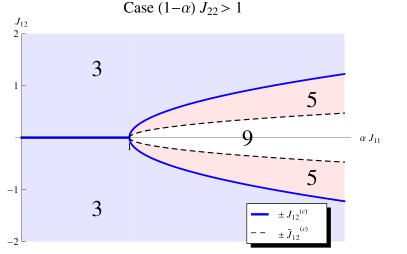
The rich scenario depicted in Theorem 2.3 can be qualitatively summarized in the phase diagrams presented in Figure 2.1, where the phase space (ฮฑโ€‹J11,J12)๐›ผsubscript๐ฝ11subscript๐ฝ12(\alpha J_{11},J_{12}) is described for a fixed value of (1โˆ’ฮฑ)โ€‹J221๐›ผsubscript๐ฝ22(1-\alpha)J_{22}. A totally analogous picture can be drawn in the converse situation when we fix ฮฑโ€‹J11๐›ผsubscript๐ฝ11\alpha J_{11} instead.

Refer to caption
Refer to caption
Figure 2.1: Picture of the phase space (ฮฑโ€‹J11,J12)๐›ผsubscript๐ฝ11subscript๐ฝ12\left(\alpha J_{11},J_{12}\right) for a fixed value of (1โˆ’ฮฑ)โ€‹J221๐›ผsubscript๐ฝ22(1-\alpha)J_{22}. Each coloured region represents a phase with as many equilibria of (11) as indicated by the numerical label. In the left panel the case (1โˆ’ฮฑ)โ€‹J22โ‰ค11๐›ผsubscript๐ฝ221(1-\alpha)J_{22}\leq 1 is illustrated. The blue separation line is |J12|=J12(c)subscript๐ฝ12superscriptsubscript๐ฝ12๐‘|J_{12}|=J_{12}^{(c)}. The right panel displays the case (1โˆ’ฮฑ)โ€‹J22>11๐›ผsubscript๐ฝ221(1-\alpha)J_{22}>1. The blue curve is still |J12|=J12(c)subscript๐ฝ12superscriptsubscript๐ฝ12๐‘|J_{12}|=J_{12}^{(c)}, while the dashed black one corresponds to |J12|=J~12(c)subscript๐ฝ12superscriptsubscript~๐ฝ12๐‘|J_{12}|=\widetilde{J}_{12}^{(c)} and it is qualitative. Indeed, the latter is defined implicitly by a tangency relation and it can be obtained numerically. More hints about this curve will be given in the proof of Theorem 2.3 in Section 3.
Remark 2.3.

Imagine to start with two independent Curie-Weiss models (J12=0subscript๐ฝ120J_{12}=0): one of size N1subscript๐‘1N_{1} and with inverse temperature ฮฑโ€‹J11โ‰ค1๐›ผsubscript๐ฝ111\alpha J_{11}\leq 1 and the other of size N2subscript๐‘2N_{2} and with inverse temperature (1โˆ’ฮฑ)โ€‹J22>11๐›ผsubscript๐ฝ221(1-\alpha)J_{22}>1. The long time behavior of the whole system is well known in this independence case: the first subsystem will converge to a disordered state, while the second one will polarize. Item (b) in Theoremย 2.3 says that if we turn on the coupling strength J12subscript๐ฝ12J_{12}, whatever its intensity is, both populations will polarize in the long run. Hence, the supercritical Curie-Weiss model creates a sort of bulk of polarization able to influence also the rest of the global population.

Remark 2.4.

If we consider the Hamiltonian (2) with h1=h2=0subscriptโ„Ž1subscriptโ„Ž20h_{1}=h_{2}=0, the associated asymptotic free energy is given by

โ„ฑโ€‹(๐‚)=โˆ’12โ€‹[ฮฑ2โ€‹J11โ€‹ฮฝ12+2โ€‹ฮฑโ€‹(1โˆ’ฮฑ)โ€‹J12โ€‹ฮฝ1โ€‹ฮฝ2+(1โˆ’ฮฑ)2โ€‹J22โ€‹ฮฝ22]+ฮฑโ€‹I(B)โ€‹(ฮฝ1)+(1โˆ’ฮฑ)โ€‹I(B)โ€‹(ฮฝ2),โ„ฑ๐‚12delimited-[]superscript๐›ผ2subscript๐ฝ11superscriptsubscript๐œˆ122๐›ผ1๐›ผsubscript๐ฝ12subscript๐œˆ1subscript๐œˆ2superscript1๐›ผ2subscript๐ฝ22superscriptsubscript๐œˆ22๐›ผsuperscript๐ผ๐ตsubscript๐œˆ11๐›ผsuperscript๐ผ๐ตsubscript๐œˆ2\mathcal{F}(\boldsymbol{\nu})=-\frac{1}{2}\left[\alpha^{2}J_{11}\nu_{1}^{2}+2\alpha(1-\alpha)J_{12}\nu_{1}\nu_{2}+(1-\alpha)^{2}J_{22}\nu_{2}^{2}\right]+\alpha I^{(B)}(\nu_{1})+(1-\alpha)I^{(B)}(\nu_{2})\,, (12)

where ๐‚โˆˆ[โˆ’1,+1]2๐‚superscript112\boldsymbol{\nu}\in[-1,+1]^{2} is a magnetization vector and the Cramรฉr entropy of a Bernoulli random variable I(B)superscript๐ผ๐ตI^{(B)} is defined as

I(B)โ€‹(ฮฝ)=1โˆ’ฮฝ2โ€‹logโก1โˆ’ฮฝ2+1+ฮฝ2โ€‹logโก1+ฮฝ2.superscript๐ผ๐ต๐œˆ1๐œˆ21๐œˆ21๐œˆ21๐œˆ2I^{(B)}(\nu)=\frac{1-\nu}{2}\log\frac{1-\nu}{2}+\frac{1+\nu}{2}\log\frac{1+\nu}{2}\,.

Rephrasing the statement of Theorem 2.3 in the terminology of statics analysis we get the classification of the critical points of the functional (12). In particular,

  • โ€ข

    the equilibria of (11) and the critical points of (12) coincide;

  • โ€ข

    being linearly stable (resp. linearly unstable) for the dynamics (11) translates into being a local minimum (resp. local maximum) for the free energy;

  • โ€ข

    saddles are saddles in both cases.

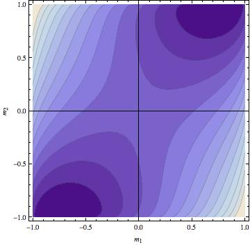
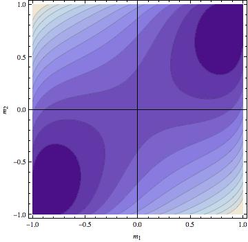
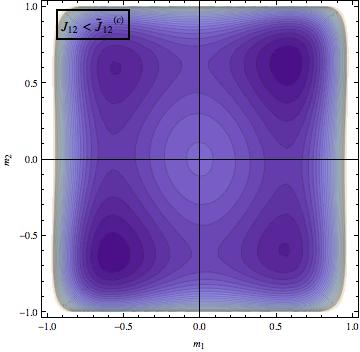
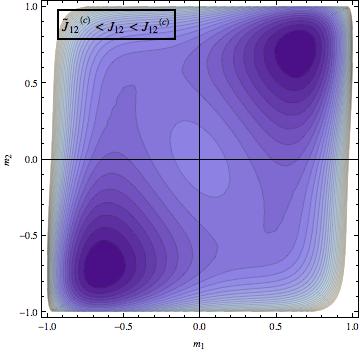
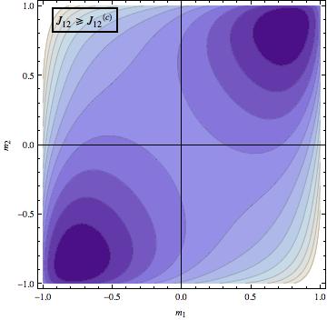
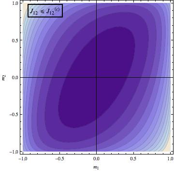
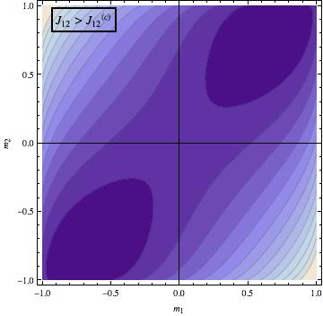
Moreover, it can be readily seen that, whenever they exist as critical points, ยฑ๐ฆ(1)plus-or-minussuperscript๐ฆ1\pm\mathbf{m}^{(1)} are the global minima for (12). In Figure 2.2 some contour plots of the free energy surface are shown.
Refer to caption
Refer to caption
(a) Case ฮฑโ€‹J11โ‰ค1๐›ผsubscript๐ฝ111\alpha J_{11}\leq 1 and (1โˆ’ฮฑ)โ€‹J22โ‰ค11๐›ผsubscript๐ฝ221(1-\alpha)J_{22}\leq 1.
Refer to caption
Refer to caption
(b) Case ฮฑโ€‹J11โ‰ค1๐›ผsubscript๐ฝ111\alpha J_{11}\leq 1 and (1โˆ’ฮฑ)โ€‹J22>11๐›ผsubscript๐ฝ221(1-\alpha)J_{22}>1 (left panel) or, conversely, case ฮฑโ€‹J11>1๐›ผsubscript๐ฝ111\alpha J_{11}>1 and (1โˆ’ฮฑ)โ€‹J22โ‰ค11๐›ผsubscript๐ฝ221(1-\alpha)J_{22}\leq 1 (right panel).

Refer to caption
Refer to caption
Refer to caption
(c) Case ฮฑโ€‹J11>1๐›ผsubscript๐ฝ111\alpha J_{11}>1 and (1โˆ’ฮฑ)โ€‹J22>11๐›ผsubscript๐ฝ221(1-\alpha)J_{22}>1.
Figure 2.2: Contour plots of the free energy surface (12) for several values of the parameters. Color scale convention: the darker the shaded region is, the lower the elevation of the surface is.

3 Proofs

3.1 Proof of Theorem 2.1

We start with a technical lemma that gives a representation of PNsubscript๐‘ƒ๐‘P_{N} (law of the process) in terms of the pair of empirical measures ๐†Nsubscript๐†๐‘\boldsymbol{\rho}_{N}.

Lemma 3.1.

It holds

dโ€‹PNdโ€‹WโŠ—Nโ€‹(ฯƒโ€‹[0,T])=expโก[Nโ€‹Fโ€‹(๐†Nโ€‹(ฯƒโ€‹[0,T]))+Oโ€‹(1)]๐‘‘subscript๐‘ƒ๐‘๐‘‘superscript๐‘Štensor-productabsent๐‘๐œŽ0๐‘‡๐‘๐นsubscript๐†๐‘๐œŽ0๐‘‡๐‘‚1\frac{dP_{N}}{dW^{\otimes N}}\left(\sigma[0,T]\right)=\exp\left[NF\left(\boldsymbol{\rho}_{N}\left(\sigma[0,T]\right)\right)+O(1)\right] (13)

where, for ๐โˆˆโ„ณ1โ€‹(๐’Ÿโ€‹[0,T])ร—โ„ณ1โ€‹(๐’Ÿโ€‹[0,T])๐subscriptโ„ณ1๐’Ÿ0๐‘‡subscriptโ„ณ1๐’Ÿ0๐‘‡\boldsymbol{Q}\in\mathscr{M}_{1}(\mathscr{D}[0,T])\times\mathscr{M}_{1}(\mathscr{D}[0,T]), Fโ€‹(๐)๐น๐F(\boldsymbol{Q}) is expressed by (6).

Proof.

The proof is basically an application of the analogous of the Girsanovโ€™s formula in the case of stochastic integrals with respect to point processes (see ย [Brรฉ81, LS01]).
The exponent in the Radon-Nikodym derivative (13) consists of two analogous terms: one related to the sum over sites belonging to population I1subscript๐ผ1I_{1} and the other to the sum over sites in I2subscript๐ผ2I_{2}. Not to be redundant we make explicit only the computations related to the first term; at each step the second is similar and will be referred to as term 2.
Let (๐’ฉt(1)โ€‹(j))jโˆˆI1subscriptsuperscriptsubscript๐’ฉ๐‘ก1๐‘—๐‘—subscript๐ผ1(\mathcal{N}_{t}^{(1)}(j))_{j\in I_{1}} (resp. (๐’ฉt(2)โ€‹(j))jโˆˆI2subscriptsuperscriptsubscript๐’ฉ๐‘ก2๐‘—๐‘—subscript๐ผ2(\mathcal{N}_{t}^{(2)}(j))_{j\in I_{2}}) be the multivariate Poisson process counting the jumps of ฯƒjsubscript๐œŽ๐‘—\sigma_{j} in population I1subscript๐ผ1I_{1} (resp. I2subscript๐ผ2I_{2}). If we read ฯƒjโ€‹(tโˆ’)=limsโ†’tโˆ’ฯƒjโ€‹(s)subscript๐œŽ๐‘—limit-from๐‘กsubscriptโ†’๐‘ limit-from๐‘กsubscript๐œŽ๐‘—๐‘ \displaystyle{\sigma_{j}(t-)=\lim_{s\rightarrow t-}\sigma_{j}(s)} and mฯ1โ€‹(tโˆ’)โ€‹(ฯƒ)=limsโ†’tโˆ’mฯ1โ€‹(s)โ€‹(ฯƒ)subscript๐‘šsubscript๐œŒ1limit-from๐‘ก๐œŽsubscriptโ†’๐‘ limit-from๐‘กsubscript๐‘šsubscript๐œŒ1๐‘ ๐œŽ\displaystyle{m_{\rho_{1}(t-)}(\sigma)=\lim_{s\rightarrow t-}m_{\rho_{1}(s)}(\sigma)}, it yields

dโ€‹PNdโ€‹WโŠ—N(ฯƒ[0,T])=exp{โˆ‘jโˆˆI1[โˆซ0T(1โˆ’eโˆ’ฯƒjโ€‹(t)โ€‹[R1โ€‹(๐ฆ๐†Nโ€‹(t)โ€‹(ฯƒ))+h1])dt+โˆซ0Tlogeโˆ’ฯƒjโ€‹(tโˆ’)โ€‹[R1โ€‹(๐ฆ๐†Nโ€‹(tโˆ’)โ€‹(ฯƒ))+h1]d๐’ฉt(1)(j)]+term 2}.๐‘‘subscript๐‘ƒ๐‘๐‘‘superscript๐‘Štensor-productabsent๐‘๐œŽ0๐‘‡subscript๐‘—subscript๐ผ1delimited-[]superscriptsubscript0๐‘‡1superscript๐‘’subscript๐œŽ๐‘—๐‘กdelimited-[]subscript๐‘…1subscript๐ฆsubscript๐†๐‘๐‘ก๐œŽsubscriptโ„Ž1๐‘‘๐‘กsuperscriptsubscript0๐‘‡superscript๐‘’subscript๐œŽ๐‘—limit-from๐‘กdelimited-[]subscript๐‘…1subscript๐ฆsubscript๐†๐‘limit-from๐‘ก๐œŽsubscriptโ„Ž1๐‘‘superscriptsubscript๐’ฉ๐‘ก1๐‘—term 2\frac{dP_{N}}{dW^{\otimes N}}\left(\sigma[0,T]\right)=\exp\Bigg{\{}\sum_{j\in I_{1}}\left[\int_{0}^{T}\left(1-e^{-\sigma_{j}(t)\left[R_{1}\left(\mathbf{m}_{\boldsymbol{\rho}_{N}(t)}(\sigma)\right)+h_{1}\right]}\right)dt\right.\\ \left.+\int_{0}^{T}\log e^{-\sigma_{j}(t-)\left[R_{1}\left(\mathbf{m}_{\boldsymbol{\rho}_{N}(t-)}(\sigma)\right)+h_{1}\right]}d\mathcal{N}_{t}^{(1)}(j)\right]+\mbox{{term 2}}\Bigg{\}}\,.

Moreover, since ฯƒ๐œŽ\sigma has no simultaneous jumps and โˆซ๐’ฉT(1)โ€‹๐‘‘ฯ1<+โˆžsubscriptsuperscript๐’ฉ1๐‘‡differential-dsubscript๐œŒ1\int\mathcal{N}^{(1)}_{T}d\rho_{1}<+\infty (resp. โˆซ๐’ฉT(2)โ€‹๐‘‘ฯ1<+โˆžsubscriptsuperscript๐’ฉ2๐‘‡differential-dsubscript๐œŒ1\int\mathcal{N}^{(2)}_{T}d\rho_{1}<+\infty) almost surely with respect to WโŠ—Nsuperscript๐‘Štensor-productabsent๐‘W^{\otimes N}, we get

dโ€‹PNdโ€‹WโŠ—N(ฯƒ[0,T])=exp{โˆ‘jโˆˆI1[โˆซ0T(1โˆ’eโˆ’ฯƒjโ€‹(t)โ€‹[R1โ€‹(๐ฆ๐†Nโ€‹(t)โ€‹(ฯƒ))+h1])dt+โˆซ0Tฯƒj(t)[R1(๐ฆ๐†Nโ€‹(t)(ฯƒ))+h1]d๐’ฉt(1)(j)+O(1N1)]+term 2}.๐‘‘subscript๐‘ƒ๐‘๐‘‘superscript๐‘Štensor-productabsent๐‘๐œŽ0๐‘‡subscript๐‘—subscript๐ผ1delimited-[]superscriptsubscript0๐‘‡1superscript๐‘’subscript๐œŽ๐‘—๐‘กdelimited-[]subscript๐‘…1subscript๐ฆsubscript๐†๐‘๐‘ก๐œŽsubscriptโ„Ž1๐‘‘๐‘กsuperscriptsubscript0๐‘‡subscript๐œŽ๐‘—๐‘กdelimited-[]subscript๐‘…1subscript๐ฆsubscript๐†๐‘๐‘ก๐œŽsubscriptโ„Ž1๐‘‘superscriptsubscript๐’ฉ๐‘ก1๐‘—๐‘‚1subscript๐‘1term 2\frac{dP_{N}}{dW^{\otimes N}}\left(\sigma[0,T]\right)=\exp\Bigg{\{}\sum_{j\in I_{1}}\left[\int_{0}^{T}\left(1-e^{-\sigma_{j}(t)\left[R_{1}\left(\mathbf{m}_{\boldsymbol{\rho}_{N}(t)}(\sigma)\right)+h_{1}\right]}\right)dt\right.\\ \left.+\int_{0}^{T}\sigma_{j}(t)\left[R_{1}\left(\mathbf{m}_{\boldsymbol{\rho}_{N}(t)}(\sigma)\right)+h_{1}\right]d\mathcal{N}_{t}^{(1)}(j)+O\left(\frac{1}{N_{1}}\right)\right]+\mbox{{term 2}}\Bigg{\}}\,.

Lastly, due to a general result for reversible spin-flip systems (we refer to ย [DPdH96], Lemmaย 3), we can write

dโ€‹PNdโ€‹WโŠ—N(ฯƒ[0,T])=exp{โˆ‘jโˆˆI1[โˆซ0T(1โˆ’eโˆ’ฯƒjโ€‹(t)โ€‹[R1โ€‹(๐ฆ๐†Nโ€‹(t)โ€‹(ฯƒ))+h1])dtโˆ’ฯƒjโ€‹(0)2[R1(๐ฆ๐†Nโ€‹(0)(ฯƒ))+h1]+ฯƒjโ€‹(T)2[R1(๐ฆ๐†Nโ€‹(T)(ฯƒ))+h1]]+term 2+O(1)}๐‘‘subscript๐‘ƒ๐‘๐‘‘superscript๐‘Štensor-productabsent๐‘๐œŽ0๐‘‡subscript๐‘—subscript๐ผ1delimited-[]superscriptsubscript0๐‘‡1superscript๐‘’subscript๐œŽ๐‘—๐‘กdelimited-[]subscript๐‘…1subscript๐ฆsubscript๐†๐‘๐‘ก๐œŽsubscriptโ„Ž1๐‘‘๐‘กsubscript๐œŽ๐‘—02delimited-[]subscript๐‘…1subscript๐ฆsubscript๐†๐‘0๐œŽsubscriptโ„Ž1subscript๐œŽ๐‘—๐‘‡2delimited-[]subscript๐‘…1subscript๐ฆsubscript๐†๐‘๐‘‡๐œŽsubscriptโ„Ž1term 2๐‘‚1\frac{dP_{N}}{dW^{\otimes N}}\left(\sigma[0,T]\right)=\exp\Bigg{\{}\sum_{j\in I_{1}}\left[\int_{0}^{T}\left(1-e^{-\sigma_{j}(t)\left[R_{1}\left(\mathbf{m}_{\boldsymbol{\rho}_{N}(t)}(\sigma)\right)+h_{1}\right]}\right)dt\right.\\ \left.-\frac{\sigma_{j}(0)}{2}\left[R_{1}\left(\mathbf{m}_{\boldsymbol{\rho}_{N}(0)}(\sigma)\right)+h_{1}\right]+\frac{\sigma_{j}(T)}{2}\left[R_{1}\left(\mathbf{m}_{\boldsymbol{\rho}_{N}(T)}(\sigma)\right)+h_{1}\right]\right]+\mbox{{term 2}}+O(1)\Bigg{\}}

and this leads us to the expression (6) for F๐นF. โˆŽ

Before proving Theorem 2.1, we need to show the following result.

Proposition 3.1.

Let ๐’ฒNโ€‹(โ‹…):=WโŠ—Nโ€‹{๐›’Nโˆˆโ‹…}assignsubscript๐’ฒ๐‘โ‹…superscript๐‘Štensor-productabsent๐‘subscript๐›’๐‘โ‹…\mathcal{W}_{N}(\cdot):=W^{\otimes N}\left\{\boldsymbol{\rho}_{N}\in\cdot\right\} be the law of ๐›’Nsubscript๐›’๐‘\boldsymbol{\rho}_{N} in the case of independence. The sequence {๐’ฒN}Nโ‰ฅ1subscriptsubscript๐’ฒ๐‘๐‘1\{\mathcal{W}_{N}\}_{N\geq 1} obeys a Large Deviation Principle (LDP) with rate function

Iโ€‹(๐‘ธ)=ฮฑโ€‹Hโ€‹(Q1|W)+(1โˆ’ฮฑ)โ€‹Hโ€‹(Q2|W).๐ผ๐‘ธ๐›ผ๐ปconditionalsubscript๐‘„1๐‘Š1๐›ผ๐ปconditionalsubscript๐‘„2๐‘ŠI(\boldsymbol{Q})=\alpha H(Q_{1}|W)+(1-\alpha)H(Q_{2}|W)\,. (14)
Proof.

Since under ๐’ฒNsubscript๐’ฒ๐‘\mathcal{W}_{N} the random variables (ฯƒjโ€‹[0,T])j=1Nsuperscriptsubscriptsubscript๐œŽ๐‘—0๐‘‡๐‘—1๐‘(\sigma_{j}[0,T])_{j=1}^{N} are i.i.d., by Sanovโ€™s Theorem (see Theorem 3.2.17 in ย [DS89]) we can deduce that the sequence {๐’ฒNi}Niโ‰ฅ1subscriptsubscript๐’ฒsubscript๐‘๐‘–subscript๐‘๐‘–1\{\mathcal{W}_{N_{i}}\}_{N_{i}\geq 1}, with ๐’ฒNiโ€‹(โ‹…)=WโŠ—Niโ€‹{ฯiโˆˆโ‹…}subscript๐’ฒsubscript๐‘๐‘–โ‹…superscript๐‘Štensor-productabsentsubscript๐‘๐‘–subscript๐œŒ๐‘–โ‹…\mathcal{W}_{N_{i}}(\cdot)=W^{\otimes N_{i}}\{\rho_{i}\in\,\cdot\}, satisfies a large deviation principle with rate function H(โ‹…|W)H(\cdot|W), for i=1,2๐‘–12i=1,2. Moreover, because of independence, if we consider A,Bโˆˆโ„ฌโ€‹(๐’Ÿโ€‹[0,T])๐ด๐ตโ„ฌ๐’Ÿ0๐‘‡A,B\in\mathcal{B}(\mathscr{D}[0,T]) Borelian sets, we get

๐’ฒNโ€‹{๐†NโˆˆAร—B}=๐’ฒN1โ€‹{ฯ1โˆˆA}โ€‹๐’ฒN2โ€‹{ฯ2โˆˆB}.subscript๐’ฒ๐‘subscript๐†๐‘๐ด๐ตsubscript๐’ฒsubscript๐‘1subscript๐œŒ1๐ดsubscript๐’ฒsubscript๐‘2subscript๐œŒ2๐ต\mathcal{W}_{N}\{\boldsymbol{\rho}_{N}\in A\times B\}=\mathcal{W}_{N_{1}}\{\rho_{1}\in A\}\,\mathcal{W}_{N_{2}}\{\rho_{2}\in B\}.

Therefore, taking closed sets C1,C2โˆˆโ„ฌโ€‹(๐’Ÿโ€‹[0,T])subscript๐ถ1subscript๐ถ2โ„ฌ๐’Ÿ0๐‘‡C_{1},C_{2}\in\mathcal{B}(\mathscr{D}[0,T]), we can estimate

lim supNโ†’+โˆž1Nโ€‹logโก๐’ฒNโ€‹(C1ร—C2)subscriptlimit-supremumโ†’๐‘1๐‘subscript๐’ฒ๐‘subscript๐ถ1subscript๐ถ2\displaystyle\limsup_{N\to+\infty}\frac{1}{N}\log\mathcal{W}_{N}(C_{1}\times C_{2}) โ‰คฮฑโ€‹lim supN1โ†’+โˆž1N1โ€‹logโก๐’ฒN1โ€‹(C1)+(1โˆ’ฮฑ)โ€‹lim supN2โ†’+โˆž1N2โ€‹logโก๐’ฒN2โ€‹(C2)absent๐›ผsubscriptlimit-supremumโ†’subscript๐‘11subscript๐‘1subscript๐’ฒsubscript๐‘1subscript๐ถ11๐›ผsubscriptlimit-supremumโ†’subscript๐‘21subscript๐‘2subscript๐’ฒsubscript๐‘2subscript๐ถ2\displaystyle\leq\alpha\limsup_{N_{1}\to+\infty}\frac{1}{N_{1}}\log\mathcal{W}_{N_{1}}(C_{1})+(1-\alpha)\limsup_{N_{2}\to+\infty}\frac{1}{N_{2}}\log\mathcal{W}_{N_{2}}(C_{2})
โ‰คโˆ’infQ1โˆˆC1Q2โˆˆC2[ฮฑโ€‹Hโ€‹(Q1|W)+(1โˆ’ฮฑ)โ€‹Hโ€‹(Q2|W)].absentsubscriptinfimumsubscript๐‘„1subscript๐ถ1subscript๐‘„2subscript๐ถ2delimited-[]๐›ผ๐ปconditionalsubscript๐‘„1๐‘Š1๐›ผ๐ปconditionalsubscript๐‘„2๐‘Š\displaystyle\leq-\inf_{\begin{subarray}{c}Q_{1}\in C_{1}\\ Q_{2}\in C_{2}\end{subarray}}\left[\alpha H(Q_{1}|W)+(1-\alpha)H(Q_{2}|W)\right]\,.

The LDP lower bound is proved similarly. โˆŽ

We are now ready to prove the large deviation principle for the laws {๐’ซN}Nโ‰ฅ1subscriptsubscript๐’ซ๐‘๐‘1\{\mathcal{P}_{N}\}_{N\geq 1} of ๐†Nsubscript๐†๐‘\boldsymbol{\rho}_{N} (under PNsubscript๐‘ƒ๐‘P_{N}) stated in Theorem 2.1. Thanks to Lemma 3.1 we have identified the Radon-Nikodym derivative that relates WโŠ—Nsuperscript๐‘Štensor-productabsent๐‘W^{\otimes N} and PNsubscript๐‘ƒ๐‘P_{N}. A natural way to develop a large deviation principle is now to rely on Proposition 3.1. Indeed, by using Lemma 3.1, we have

๐’ซNโ€‹(โ‹…)=โˆซ๐Ÿ™{๐†Nโˆˆโ‹…}โ€‹๐‘‘PN=โˆซexpโก[Nโ€‹Fโ€‹(๐†N)]โ€‹โ€‰1{๐†Nโˆˆโ‹…}โ€‹๐‘‘WโŠ—N=โˆซexpโก[Nโ€‹Fโ€‹(๐‘ธ)]โ€‹โ€‰1{๐‘ธโˆˆโ‹…}โ€‹๐’ฒNโ€‹(dโ€‹๐‘ธ),subscript๐’ซ๐‘โ‹…subscript1subscript๐†๐‘โ‹…differential-dsubscript๐‘ƒ๐‘๐‘๐นsubscript๐†๐‘subscript1subscript๐†๐‘โ‹…differential-dsuperscript๐‘Štensor-productabsent๐‘๐‘๐น๐‘ธsubscript1๐‘ธโ‹…subscript๐’ฒ๐‘๐‘‘๐‘ธ\mathcal{P}_{N}(\cdot)=\int\mathds{1}_{\{\boldsymbol{\rho}_{N}\in\;\cdot\}}\,dP_{N}\\ =\int\exp[NF(\boldsymbol{\rho}_{N})]\,\mathds{1}_{\{\boldsymbol{\rho}_{N}\in\;\cdot\}}\,dW^{\otimes N}\\ =\int\exp[NF(\boldsymbol{Q})]\,\mathds{1}_{\{\boldsymbol{Q}\in\;\cdot\}}\,\mathcal{W}_{N}(d\boldsymbol{Q})\,,

with ๐‘ธ=๐†N๐‘ธsubscript๐†๐‘\boldsymbol{Q}=\boldsymbol{\rho}_{N}. This means that

dโ€‹๐’ซNdโ€‹๐’ฒNโ€‹(๐‘ธ)=expโก[Nโ€‹Fโ€‹(๐‘ธ)].๐‘‘subscript๐’ซ๐‘๐‘‘subscript๐’ฒ๐‘๐‘ธ๐‘๐น๐‘ธ\frac{d\mathcal{P}_{N}}{d\mathcal{W}_{N}}(\boldsymbol{Q})=\exp[NF(\boldsymbol{Q})]\,. (15)

Equation (15) allows us to apply Varadhanโ€™s Lemma (see Theorem 2.2 in ย [Var84]) and conclude that the LDP for {๐’ฒN}Nโ‰ฅ1subscriptsubscript๐’ฒ๐‘๐‘1\{\mathcal{W}_{N}\}_{N\geq 1} with rate function Iโ€‹(๐‘ธ)๐ผ๐‘ธI(\boldsymbol{Q}) implies the LDP for {๐’ซN}Nโ‰ฅ1subscriptsubscript๐’ซ๐‘๐‘1\{\mathcal{P}_{N}\}_{N\geq 1} with rate function Iโ€‹(๐‘ธ)โˆ’Fโ€‹(๐‘ธ)๐ผ๐‘ธ๐น๐‘ธI(\boldsymbol{Q})-F(\boldsymbol{Q}), where Iโ€‹(โ‹…)๐ผโ‹…I(\cdot) and Fโ€‹(โ‹…)๐นโ‹…F(\cdot) are defined by equations (14) and (6), respectively.

3.2 Proof of Theorem 2.2

We need to define a new process and to derive a technical lemma related to it.
Given ๐‘ธโˆˆโ„ณ1โ€‹(๐’Ÿโ€‹[0,T])ร—โ„ณ1โ€‹(๐’Ÿโ€‹[0,T])๐‘ธsubscriptโ„ณ1๐’Ÿ0๐‘‡subscriptโ„ณ1๐’Ÿ0๐‘‡\boldsymbol{Q}\in\mathscr{M}_{1}(\mathscr{D}[0,T])\times\mathscr{M}_{1}(\mathscr{D}[0,T]), we can associate with ๐‘ธ๐‘ธ\boldsymbol{Q} a pair (ฮท(1)โ€‹(t),ฮท(2)โ€‹(t))tโˆˆ[0,T]subscriptsuperscript๐œ‚1๐‘กsuperscript๐œ‚2๐‘ก๐‘ก0๐‘‡\left(\eta^{(1)}(t),\eta^{(2)}(t)\right)_{t\in[0,T]} of independent Markov processes both with state space ๐’ฎ๐’ฎ\mathscr{S}, initial distribution ฮป๐œ†\lambda and with respective time-dependent infinitesimal generators โ„’1๐‘ธsuperscriptsubscriptโ„’1๐‘ธ\mathcal{L}_{1}^{\boldsymbol{Q}} and โ„’2๐‘ธsuperscriptsubscriptโ„’2๐‘ธ\mathcal{L}_{2}^{\boldsymbol{Q}}, acting on functions from ๐’ฎ๐’ฎ\mathscr{S} to โ„โ„\mathbb{R} as

โ„’1๐‘ธโ€‹fโ€‹(ฮท)superscriptsubscriptโ„’1๐‘ธ๐‘“๐œ‚\displaystyle\mathcal{L}_{1}^{\boldsymbol{Q}}f\left(\eta\right) =eโˆ’ฮทโ€‹[R1โ€‹(๐ฆ๐‘ธโ€‹(t)โ€‹(ฮท))+h1]โ€‹โˆ‡ฮทfโ€‹(ฮท)absentsuperscript๐‘’๐œ‚delimited-[]subscript๐‘…1subscript๐ฆ๐‘ธ๐‘ก๐œ‚subscriptโ„Ž1superscriptโˆ‡๐œ‚๐‘“๐œ‚\displaystyle=e^{-\eta\left[R_{1}\left(\mathbf{m}_{\boldsymbol{Q}(t)}\left(\eta\right)\right)+h_{1}\right]}\,\nabla^{\eta}f\left(\eta\right)
โ„’2๐‘ธโ€‹fโ€‹(ฮท)superscriptsubscriptโ„’2๐‘ธ๐‘“๐œ‚\displaystyle\mathcal{L}_{2}^{\boldsymbol{Q}}f\left(\eta\right) =eโˆ’ฮทโ€‹[R2โ€‹(๐ฆ๐‘ธโ€‹(t)โ€‹(ฮท))+h2]โ€‹โˆ‡ฮทfโ€‹(ฮท).absentsuperscript๐‘’๐œ‚delimited-[]subscript๐‘…2subscript๐ฆ๐‘ธ๐‘ก๐œ‚subscriptโ„Ž2superscriptโˆ‡๐œ‚๐‘“๐œ‚\displaystyle=e^{-\eta\left[R_{2}\left(\mathbf{m}_{\boldsymbol{Q}(t)}\left(\eta\right)\right)+h_{2}\right]}\,\nabla^{\eta}f\left(\eta\right).

Let Pi๐‘ธsubscriptsuperscript๐‘ƒ๐‘ธ๐‘–P^{\boldsymbol{Q}}_{i} be the distribution of the process (ฮท(i)โ€‹(t))tโˆˆ[0,T]subscriptsuperscript๐œ‚๐‘–๐‘ก๐‘ก0๐‘‡\left(\eta^{(i)}(t)\right)_{t\in[0,T]}, with i=1,2๐‘–12i=1,2, then the joint law of the pair (ฮท(1)โ€‹(t),ฮท(2)โ€‹(t))tโˆˆ[0,T]subscriptsuperscript๐œ‚1๐‘กsuperscript๐œ‚2๐‘ก๐‘ก0๐‘‡\left(\eta^{(1)}(t),\eta^{(2)}(t)\right)_{t\in[0,T]} is denoted by ๐‘ท๐‘ธ=P1๐‘ธโŠ—P2๐‘ธsuperscript๐‘ท๐‘ธtensor-productsubscriptsuperscript๐‘ƒ๐‘ธ1subscriptsuperscript๐‘ƒ๐‘ธ2\boldsymbol{P}^{\boldsymbol{Q}}=P^{\boldsymbol{Q}}_{1}\otimes P^{\boldsymbol{Q}}_{2}.
Next proposition shows a very important property of ๐‘ท๐‘ธsuperscript๐‘ท๐‘ธ\boldsymbol{P}^{\boldsymbol{Q}}.

Proposition 3.2.

For every ๐โˆˆโ„ณ1โ€‹(๐’Ÿโ€‹[0,T])ร—โ„ณ1โ€‹(๐’Ÿโ€‹[0,T])๐subscriptโ„ณ1๐’Ÿ0๐‘‡subscriptโ„ณ1๐’Ÿ0๐‘‡\boldsymbol{Q}\in\mathscr{M}_{1}(\mathscr{D}[0,T])\times\mathscr{M}_{1}(\mathscr{D}[0,T]) such that โ„โ€‹(๐)<+โˆžโ„๐\mathcal{I}(\boldsymbol{Q})<+\infty,

โ„โ€‹(๐‘ธ)=ฮฑโ€‹Hโ€‹(Q1|P1๐‘ธ)+(1โˆ’ฮฑ)โ€‹Hโ€‹(Q2|P2๐‘ธ).โ„๐‘ธ๐›ผ๐ปconditionalsubscript๐‘„1subscriptsuperscript๐‘ƒ๐‘ธ11๐›ผ๐ปconditionalsubscript๐‘„2subscriptsuperscript๐‘ƒ๐‘ธ2\mathcal{I}(\boldsymbol{Q})=\alpha H\left(Q_{1}\left|P^{\boldsymbol{Q}}_{1}\right.\right)+(1-\alpha)H\left(Q_{2}\left|P^{\boldsymbol{Q}}_{2}\right.\right)\,. (16)
Proof.

Similarly to the proof of Lemma 3.1, by Girsanovโ€™s formula for Markov processes and reversibility, it is easy to verify that the following representations for F1โ€‹(Q1)subscript๐น1subscript๐‘„1F_{1}(Q_{1}) and F2โ€‹(Q2)subscript๐น2subscript๐‘„2F_{2}(Q_{2}) (defined in (7)) hold

Fiโ€‹(Qi)=โˆซ๐‘‘Qiโ€‹(ฮท(i)โ€‹[0,T])โ€‹logโกdโ€‹Pi๐‘ธdโ€‹Wโ€‹(ฮท(i)โ€‹[0,T])ย forย โ€‹i=1,2.formulae-sequencesubscript๐น๐‘–subscript๐‘„๐‘–differential-dsubscript๐‘„๐‘–superscript๐œ‚๐‘–0๐‘‡๐‘‘subscriptsuperscript๐‘ƒ๐‘ธ๐‘–๐‘‘๐‘Šsuperscript๐œ‚๐‘–0๐‘‡ย forย ๐‘–12F_{i}(Q_{i})=\int dQ_{i}\left(\eta^{(i)}[0,T]\right)\log\frac{dP^{\boldsymbol{Q}}_{i}}{dW}\left(\eta^{(i)}[0,T]\right)\quad\mbox{ for }i=1,2.

By combining what we obtained, we can compute

โ„โ€‹(๐‘ธ)โ„๐‘ธ\displaystyle\mathcal{I}(\boldsymbol{Q}) =ฮฑโ€‹[Hโ€‹(Q1|W)โˆ’F1โ€‹(Q1)]+(1โˆ’ฮฑ)โ€‹[Hโ€‹(Q2|W)โˆ’F2โ€‹(Q2)]absent๐›ผdelimited-[]๐ปconditionalsubscript๐‘„1๐‘Šsubscript๐น1subscript๐‘„11๐›ผdelimited-[]๐ปconditionalsubscript๐‘„2๐‘Šsubscript๐น2subscript๐‘„2\displaystyle=\alpha\left[H(Q_{1}|W)-F_{1}(Q_{1})\right]+(1-\alpha)\left[H(Q_{2}|W)-F_{2}(Q_{2})\right]
=ฮฑโ€‹[โˆซ๐‘‘Q1โ€‹logโกdโ€‹Q1dโ€‹Wโˆ’โˆซ๐‘‘Q1โ€‹logโกdโ€‹P1๐‘ธdโ€‹W]+(1โˆ’ฮฑ)โ€‹[โˆซ๐‘‘Q2โ€‹logโกdโ€‹Q2dโ€‹Wโˆ’โˆซ๐‘‘Q2โ€‹logโกdโ€‹P2๐‘ธdโ€‹W]absent๐›ผdelimited-[]differential-dsubscript๐‘„1๐‘‘subscript๐‘„1๐‘‘๐‘Šdifferential-dsubscript๐‘„1๐‘‘subscriptsuperscript๐‘ƒ๐‘ธ1๐‘‘๐‘Š1๐›ผdelimited-[]differential-dsubscript๐‘„2๐‘‘subscript๐‘„2๐‘‘๐‘Šdifferential-dsubscript๐‘„2๐‘‘subscriptsuperscript๐‘ƒ๐‘ธ2๐‘‘๐‘Š\displaystyle=\alpha\left[\int dQ_{1}\log\frac{dQ_{1}}{dW}-\int dQ_{1}\log\frac{dP^{\boldsymbol{Q}}_{1}}{dW}\right]+(1-\alpha)\left[\int dQ_{2}\log\frac{dQ_{2}}{dW}-\int dQ_{2}\log\frac{dP^{\boldsymbol{Q}}_{2}}{dW}\right]
=ฮฑโ€‹Hโ€‹(Q1|P1๐‘ธ)+(1โˆ’ฮฑ)โ€‹Hโ€‹(Q2|P2๐‘ธ).absent๐›ผ๐ปconditionalsubscript๐‘„1subscriptsuperscript๐‘ƒ๐‘ธ11๐›ผ๐ปconditionalsubscript๐‘„2subscriptsuperscript๐‘ƒ๐‘ธ2\displaystyle=\alpha H\left(Q_{1}\left|P^{\boldsymbol{Q}}_{1}\right.\right)+(1-\alpha)H\left(Q_{2}\left|P^{\boldsymbol{Q}}_{2}\right.\right)\,.

โˆŽ

We can now conclude the proof of Theorem 2.2.
By properness of the relative entropy, from (16) we have that โ„โ€‹(๐‘ธ)=0โ„๐‘ธ0\mathcal{I}(\boldsymbol{Q})=0 is equivalent to ๐‘ธ=๐‘ท๐‘ธ๐‘ธsuperscript๐‘ท๐‘ธ\boldsymbol{Q}=\boldsymbol{P^{Q}}. Let us suppose ๐‘ธโˆ—superscript๐‘ธ\boldsymbol{Q}^{*} is a solution of this last equation. Then, in particular, ๐’’โ€‹(t)=๐‘ธโˆ—โ€‹(t)=๐‘ท๐‘ธโˆ—โ€‹(t)๐’’๐‘กsuperscript๐‘ธ๐‘กsuperscript๐‘ทsuperscript๐‘ธ๐‘ก\boldsymbol{q}(t)=\boldsymbol{Q}^{*}(t)=\boldsymbol{P}^{\boldsymbol{Q}^{*}}(t). The marginals of a Markov process are solutions of the corresponding forward equation that, in this case, leads to the fact that ๐’’โ€‹(t)๐’’๐‘ก\boldsymbol{q}(t) is a solution of (10). This differential equation, being an equation in finite dimension with locally Lipschitz coefficients, has at most one solution in [0,T]0๐‘‡[0,T]. Since ๐‘ท๐‘ธโˆ—superscript๐‘ทsuperscript๐‘ธ\boldsymbol{P}^{\boldsymbol{Q}^{*}} is totally determined by the flow ๐’’โ€‹(t)๐’’๐‘ก\boldsymbol{q}(t), it follows that equation ๐‘ธ=๐‘ท๐‘ธ๐‘ธsuperscript๐‘ท๐‘ธ\boldsymbol{Q}=\boldsymbol{P^{Q}} has at most one solution. The existence of a solution derives from the fact that โ„โ€‹(๐‘ธ)โ„๐‘ธ\mathcal{I}(\boldsymbol{Q}) is the rate function of a large deviation principle and therefore it must have at least one zero.
It remains to prove the convergence of ๐†Nsubscript๐†๐‘\boldsymbol{\rho}_{N} (law of large numbers). Let O๐‘‚O be an arbitrary open neighborhood of ๐‘ธโˆ—superscript๐‘ธ\boldsymbol{Q}^{*} in โ„ณ1โ€‹(๐’Ÿโ€‹[0,T])ร—โ„ณ1โ€‹(๐’Ÿโ€‹[0,T])subscriptโ„ณ1๐’Ÿ0๐‘‡subscriptโ„ณ1๐’Ÿ0๐‘‡\mathscr{M}_{1}(\mathscr{D}[0,T])\times\mathscr{M}_{1}(\mathscr{D}[0,T]). By the lower semi-continuity of โ„โ€‹(โ‹…)โ„โ‹…\mathcal{I}(\cdot) and the compactness of its level-sets a standard argument shows that Kโ€‹(O):=inf๐‘ธโˆ‰Oโ„โ€‹(๐‘ธ)>0assign๐พ๐‘‚subscriptinfimum๐‘ธ๐‘‚โ„๐‘ธ0K(O):=\inf_{\boldsymbol{Q}\notin O}\mathcal{I}(\boldsymbol{Q})>0. By the large deviation upper bound in Theorem 2.1 (type (9a)) there exists a positive constant A๐ดA such that

๐’ซNโ€‹(๐†Nโˆ‰O)โ‰คAโ€‹eโˆ’Nโ€‹Kโ€‹(O),subscript๐’ซ๐‘subscript๐†๐‘๐‘‚๐ดsuperscript๐‘’๐‘๐พ๐‘‚\mathcal{P}_{N}(\boldsymbol{\rho}_{N}\notin O)\leq Ae^{-NK(O)}\,,

thus giving convergence to zero with exponential decay.

3.3 Proof of Theorem 2.3

Let Vโ€‹(๐ฑ)=(2โ€‹sinhโก[R1โ€‹(๐ฑ)]โˆ’2โ€‹x1โ€‹coshโก[R1โ€‹(๐ฑ)],2โ€‹sinhโก[R2โ€‹(๐ฑ)]โˆ’2โ€‹x2โ€‹coshโก[R2โ€‹(๐ฑ)])๐‘‰๐ฑ2subscript๐‘…1๐ฑ2subscript๐‘ฅ1subscript๐‘…1๐ฑ2subscript๐‘…2๐ฑ2subscript๐‘ฅ2subscript๐‘…2๐ฑV\left(\mathbf{x}\right)=\left(2\sinh\left[R_{1}\left(\mathbf{x}\right)\right]-2x_{1}\cosh\left[R_{1}\left(\mathbf{x}\right)\right],2\sinh\left[R_{2}\left(\mathbf{x}\right)\right]-2x_{2}\cosh\left[R_{2}\left(\mathbf{x}\right)\right]\right). Under our assumptions, we must discuss existence and linear stability of equilibrium solutions for the differential system ๐ฆห™โ€‹(t)=Vโ€‹(๐ฆโ€‹(t))ห™๐ฆ๐‘ก๐‘‰๐ฆ๐‘ก\dot{\mathbf{m}}(t)=V\left(\mathbf{m}(t)\right).

Existence of stationary solutions. Denote by ๐ฆโˆ—superscript๐ฆ\mathbf{m}^{*} a pair such that Vโ€‹(๐ฆโˆ—)=๐ŸŽ๐‘‰superscript๐ฆ0V\left(\mathbf{m}^{*}\right)=\boldsymbol{0}. Any stationary point is then implicitly defined by

m1โˆ—=tanhโก[ฮฑโ€‹J11โ€‹m1โˆ—+(1โˆ’ฮฑ)โ€‹J12โ€‹m2โˆ—]m2โˆ—=tanhโก[ฮฑโ€‹J12โ€‹m1โˆ—+(1โˆ’ฮฑ)โ€‹J22โ€‹m2โˆ—].superscriptsubscript๐‘š1๐›ผsubscript๐ฝ11superscriptsubscript๐‘š11๐›ผsubscript๐ฝ12superscriptsubscript๐‘š2superscriptsubscript๐‘š2๐›ผsubscript๐ฝ12superscriptsubscript๐‘š11๐›ผsubscript๐ฝ22superscriptsubscript๐‘š2\begin{array}[]{l}m_{1}^{*}=\tanh\left[\alpha J_{11}m_{1}^{*}+(1-\alpha)J_{12}m_{2}^{*}\right]\\ m_{2}^{*}=\tanh\left[\alpha J_{12}m_{1}^{*}+(1-\alpha)J_{22}m_{2}^{*}\right].\end{array} (17)

By inverting equations (17) when J12โ‰ 0subscript๐ฝ120J_{12}\neq 0 (i.e. the model does not degenerate into two independent Curie-Weiss models), we get

m2โˆ—superscriptsubscript๐‘š2\displaystyle m_{2}^{*} =1(1โˆ’ฮฑ)โ€‹J12โ€‹[arctanhโ€‹(m1โˆ—)โˆ’ฮฑโ€‹J11โ€‹m1โˆ—]absent11๐›ผsubscript๐ฝ12delimited-[]arctanhsuperscriptsubscript๐‘š1๐›ผsubscript๐ฝ11superscriptsubscript๐‘š1\displaystyle=\frac{1}{(1-\alpha)J_{12}}\left[\mathrm{arctanh}\left(m_{1}^{*}\right)-\alpha J_{11}m_{1}^{*}\right] (ฮณ1subscript๐›พ1\gamma_{1})
m1โˆ—superscriptsubscript๐‘š1\displaystyle m_{1}^{*} =1ฮฑโ€‹J12โ€‹[arctanhโ€‹(m2โˆ—)โˆ’(1โˆ’ฮฑ)โ€‹J22โ€‹m2โˆ—].absent1๐›ผsubscript๐ฝ12delimited-[]arctanhsuperscriptsubscript๐‘š21๐›ผsubscript๐ฝ22superscriptsubscript๐‘š2\displaystyle=\frac{1}{\alpha J_{12}}\left[\mathrm{arctanh}\left(m_{2}^{*}\right)-(1-\alpha)J_{22}m_{2}^{*}\right]. (ฮณ2subscript๐›พ2\gamma_{2})

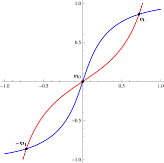
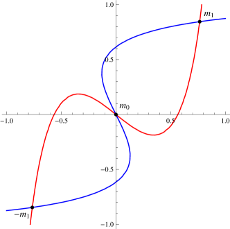
The points that verify simultaneously the two equations are the intersections of the curve ฮณ1โ€‹(m1โˆ—)subscript๐›พ1superscriptsubscript๐‘š1\gamma_{1}\left(m_{1}^{*}\right), the graph of the function m2โˆ—โ€‹(m1โˆ—)superscriptsubscript๐‘š2superscriptsubscript๐‘š1m_{2}^{*}\left(m_{1}^{*}\right), with the curve ฮณ2โ€‹(m2โˆ—)subscript๐›พ2superscriptsubscript๐‘š2\gamma_{2}\left(m_{2}^{*}\right), the graph of the function m1โˆ—โ€‹(m2โˆ—)superscriptsubscript๐‘š1superscriptsubscript๐‘š2m_{1}^{*}\left(m_{2}^{*}\right). To detect such points we use a graphical approach.
Observe that it suffices to consider J12>0subscript๐ฝ120J_{12}>0, since the complementary case can be obtained by symmetry about the vertical axis because of the oddness of the involved functions. From now on we restrict to this range of the parameter J12subscript๐ฝ12J_{12}.
A quick analysis shows the curves ฮณ1subscript๐›พ1\gamma_{1} and ฮณ2subscript๐›พ2\gamma_{2} are characterized by the following features (meant on the (m1โˆ—,m2โˆ—)superscriptsubscript๐‘š1superscriptsubscript๐‘š2(m_{1}^{*},m_{2}^{*}) plane for ฮณ1subscript๐›พ1\gamma_{1}, whilst on the (m2โˆ—,m1โˆ—)superscriptsubscript๐‘š2superscriptsubscript๐‘š1(m_{2}^{*},m_{1}^{*}) one for ฮณ2subscript๐›พ2\gamma_{2}):

  • โ€ข

    they are defined over [โˆ’1,+1]11[-1,+1] and they are odd functions;

  • โ€ข

    they diverge to ยฑโˆžplus-or-minus\pm\infty as the corresponding independent variable tends to ยฑ1plus-or-minus1\pm 1;

  • โ€ข
    (ฮณ1)subscript๐›พ1(\gamma_{1})
    1. (I)

      if ฮฑโ€‹J11โ‰ค1๐›ผsubscript๐ฝ111\alpha J_{11}\leq 1, then ฮณ1subscript๐›พ1\gamma_{1} is increasing for all values m1โˆ—โˆˆ[โˆ’1,+1]superscriptsubscript๐‘š111m_{1}^{*}\in[-1,+1];

    2. (II)

      if ฮฑโ€‹J11>1๐›ผsubscript๐ฝ111\alpha J_{11}>1, then ฮณ1subscript๐›พ1\gamma_{1} is increasing for m1โˆ—โ‰คโˆ’1โˆ’1ฮฑโ€‹J11superscriptsubscript๐‘š111๐›ผsubscript๐ฝ11m_{1}^{*}\leq-\sqrt{1-\frac{1}{\alpha J_{11}}} or for m1โˆ—โ‰ฅ1โˆ’1ฮฑโ€‹J11superscriptsubscript๐‘š111๐›ผsubscript๐ฝ11m_{1}^{*}\geq\sqrt{1-\frac{1}{\alpha J_{11}}}. Moreover, m1โˆ—=โˆ’1โˆ’1ฮฑโ€‹J11superscriptsubscript๐‘š111๐›ผsubscript๐ฝ11m_{1}^{*}=-\sqrt{1-\frac{1}{\alpha J_{11}}} and m1โˆ—=1โˆ’1ฮฑโ€‹J11superscriptsubscript๐‘š111๐›ผsubscript๐ฝ11m_{1}^{*}=\sqrt{1-\frac{1}{\alpha J_{11}}} correspond to a local maximum and minimum for ฮณ1subscript๐›พ1\gamma_{1}, respectively.

    (ฮณ2)subscript๐›พ2(\gamma_{2})
    1. (I)

      if (1โˆ’ฮฑ)โ€‹J22โ‰ค11๐›ผsubscript๐ฝ221(1-\alpha)J_{22}\leq 1, then ฮณ2subscript๐›พ2\gamma_{2} is increasing for all values m2โˆ—โˆˆ[โˆ’1,+1]superscriptsubscript๐‘š211m_{2}^{*}\in[-1,+1];

    2. (II)

      if (1โˆ’ฮฑ)โ€‹J22>11๐›ผsubscript๐ฝ221(1-\alpha)J_{22}>1, then ฮณ2subscript๐›พ2\gamma_{2} is increasing for m2โˆ—โ‰คโˆ’1โˆ’1(1โˆ’ฮฑ)โ€‹J22superscriptsubscript๐‘š2111๐›ผsubscript๐ฝ22m_{2}^{*}\leq-\sqrt{1-\frac{1}{(1-\alpha)J_{22}}} or for m2โˆ—โ‰ฅ1โˆ’1(1โˆ’ฮฑ)โ€‹J22superscriptsubscript๐‘š2111๐›ผsubscript๐ฝ22m_{2}^{*}\geq\sqrt{1-\frac{1}{(1-\alpha)J_{22}}}. Moreover, m2โˆ—=โˆ’1โˆ’1(1โˆ’ฮฑ)โ€‹J22superscriptsubscript๐‘š2111๐›ผsubscript๐ฝ22m_{2}^{*}=-\sqrt{1-\frac{1}{(1-\alpha)J_{22}}} and m2โˆ—=1โˆ’1(1โˆ’ฮฑ)โ€‹J22superscriptsubscript๐‘š2111๐›ผsubscript๐ฝ22m_{2}^{*}=\sqrt{1-\frac{1}{(1-\alpha)J_{22}}} correspond to a local maximum and minimum for ฮณ2subscript๐›พ2\gamma_{2}, respectively.

  • โ€ข

    they are convex for positive abscissas and concave for negative ones with a unique inflection point at the origin.

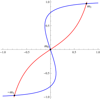
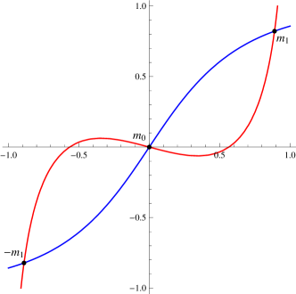
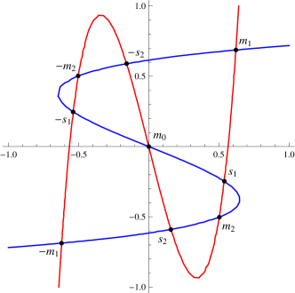
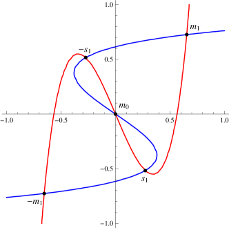
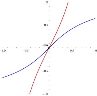
If we put the graphs ฮณ1subscript๐›พ1\gamma_{1} and ฮณ2subscript๐›พ2\gamma_{2} (after a ninety degrees clockwise rotation and a reflection about the horizontal axis) in the same (m1โˆ—,m2โˆ—)superscriptsubscript๐‘š1superscriptsubscript๐‘š2(m_{1}^{*},m_{2}^{*}) coordinate system, it is possible to understand how many times the two curves intersect depending on the parameters. We must match in all possible ways their shapes, determined by conditions (ฮณ1โˆ’I&Iโ€‹I)subscript๐›พ1๐ผ๐ผ๐ผ(\gamma_{1}-I\&II) and (ฮณ2โˆ’I&Iโ€‹I)subscript๐›พ2๐ผ๐ผ๐ผ(\gamma_{2}-I\&II). See Figureย 3.3 for an example. This leads to the number of solutions of (17).
Refer to caption
Refer to caption
(a) Case ฮฑโ€‹J11โ‰ค1๐›ผsubscript๐ฝ111\alpha J_{11}\leq 1 and (1โˆ’ฮฑ)โ€‹J22โ‰ค11๐›ผsubscript๐ฝ221(1-\alpha)J_{22}\leq 1.
Refer to caption
Refer to caption
(b) Case ฮฑโ€‹J11โ‰ค1๐›ผsubscript๐ฝ111\alpha J_{11}\leq 1 and (1โˆ’ฮฑ)โ€‹J22>11๐›ผsubscript๐ฝ221(1-\alpha)J_{22}>1 (left panel) or, conversely, case ฮฑโ€‹J11>1๐›ผsubscript๐ฝ111\alpha J_{11}>1 and (1โˆ’ฮฑ)โ€‹J22โ‰ค11๐›ผsubscript๐ฝ221(1-\alpha)J_{22}\leq 1 (right panel).

Refer to caption
Refer to caption
Refer to caption
(c) Case ฮฑโ€‹J11>1๐›ผsubscript๐ฝ111\alpha J_{11}>1 and (1โˆ’ฮฑ)โ€‹J22>11๐›ผsubscript๐ฝ221(1-\alpha)J_{22}>1.
Figure 3.3: Plot of the curves ฮณ1subscript๐›พ1\gamma_{1} (โ€”) and ฮณ2subscript๐›พ2\gamma_{2} (โ€”) for different values of the parameters.

Now we focus on the critical thresholds for the transitions a(i)โ€“a(ii), c(i)โ€“c(ii) and c(ii)โ€“c(iii) in the statement of Theoremย 2.3. Before to continue we introduce the following notation: here and in the sequel of the proof, by abuse of notation, we will denote by ฮณ2โˆ’1โ€‹(m1โˆ—)superscriptsubscript๐›พ21superscriptsubscript๐‘š1\gamma_{2}^{-1}(m_{1}^{*}) a local inverse of ฮณ2โ€‹(m2โˆ—)subscript๐›พ2superscriptsubscript๐‘š2\gamma_{2}(m_{2}^{*}); we intend ฮณ2โˆ’1superscriptsubscript๐›พ21\gamma_{2}^{-1} to be defined over a suitable monotonicity interval that may change from case to case.

Transition in (a).

A simple convexity argument shows that to know the number of intersections between ฮณ1subscript๐›พ1\gamma_{1} and ฮณ2subscript๐›พ2\gamma_{2} we must control the slope of the two curves at the origin. In particular, since ฮณ1โ€ฒโ€‹(0)=1โˆ’ฮฑโ€‹J11(1โˆ’ฮฑ)โ€‹J12superscriptsubscript๐›พ1โ€ฒ01๐›ผsubscript๐ฝ111๐›ผsubscript๐ฝ12\gamma_{1}^{\prime}(0)=\frac{1-\alpha J_{11}}{(1-\alpha)J_{12}} and (ฮณ2โˆ’1)โ€ฒโ€‹(0)=ฮฑโ€‹J121โˆ’(1โˆ’ฮฑ)โ€‹J22superscriptsuperscriptsubscript๐›พ21โ€ฒ0๐›ผsubscript๐ฝ1211๐›ผsubscript๐ฝ22\left(\gamma_{2}^{-1}\right)^{\prime}(0)=\frac{\alpha J_{12}}{1-(1-\alpha)J_{22}}, it yields

  • โ€ข

    if ฮณ1โ€ฒโ€‹(0)โ‰ฅ(ฮณ2โˆ’1)โ€ฒโ€‹(0)โ‡”J12โ‰ค(1โˆ’ฮฑโ€‹J11)โ€‹(1โˆ’(1โˆ’ฮฑ)โ€‹J22)ฮฑโ€‹(1โˆ’ฮฑ)โ‡”superscriptsubscript๐›พ1โ€ฒ0superscriptsuperscriptsubscript๐›พ21โ€ฒ0subscript๐ฝ121๐›ผsubscript๐ฝ1111๐›ผsubscript๐ฝ22๐›ผ1๐›ผ\gamma_{1}^{\prime}(0)\geq\left(\gamma_{2}^{-1}\right)^{\prime}(0)\Leftrightarrow J_{12}\leq\sqrt{\frac{(1-\alpha J_{11})(1-(1-\alpha)J_{22})}{\alpha(1-\alpha)}}, there exists a unique intersection, which is the origin;

  • โ€ข

    if ฮณ1โ€ฒโ€‹(0)<(ฮณ2โˆ’1)โ€ฒโ€‹(0)โ‡”J12>(1โˆ’ฮฑโ€‹J11)โ€‹(1โˆ’(1โˆ’ฮฑ)โ€‹J22)ฮฑโ€‹(1โˆ’ฮฑ)โ‡”superscriptsubscript๐›พ1โ€ฒ0superscriptsuperscriptsubscript๐›พ21โ€ฒ0subscript๐ฝ121๐›ผsubscript๐ฝ1111๐›ผsubscript๐ฝ22๐›ผ1๐›ผ\gamma_{1}^{\prime}(0)<\left(\gamma_{2}^{-1}\right)^{\prime}(0)\Leftrightarrow J_{12}>\sqrt{\frac{(1-\alpha J_{11})(1-(1-\alpha)J_{22})}{\alpha(1-\alpha)}}, beyond the origin, two further symmetric intersections ยฑ๐ฆ(1)plus-or-minussuperscript๐ฆ1\pm\mathbf{m}^{(1)} arise.

Transitions in (c).

Observe that ฮณ1โ€ฒโ€‹(0)superscriptsubscript๐›พ1โ€ฒ0\gamma_{1}^{\prime}(0) is an increasing function of J12subscript๐ฝ12J_{12}. On the contrary, (ฮณ2โˆ’1)โ€ฒโ€‹(0)superscriptsuperscriptsubscript๐›พ21โ€ฒ0\left(\gamma_{2}^{-1}\right)^{\prime}(0) is decreasing with respect to the same quantity. Therefore, by convexity again we can easily conclude that, for J12โ‰ฅJ12(c)subscript๐ฝ12superscriptsubscript๐ฝ12๐‘J_{12}\geq J_{12}^{(c)}, ฮณ1subscript๐›พ1\gamma_{1} and ฮณ2subscript๐›พ2\gamma_{2} must intersect three times. The transition c(ii)โ€“c(iii) remains thus proved.
We deal now with the passage c(i)โ€“c(ii). For the sake of clarity and to be able to refer to Figureย 2.1, without loss of generality, we fix (1โˆ’ฮฑ)โ€‹J22>11๐›ผsubscript๐ฝ221(1-\alpha)J_{22}>1. When J12<J12(c)subscript๐ฝ12superscriptsubscript๐ฝ12๐‘J_{12}<J_{12}^{(c)}, we may have five or nine intersections depending on the relative height of wells of the curves (monotonically tuned by the parameter J12subscript๐ฝ12J_{12}). In particular, the boundary between the two phases is determined by the tangency condition between ฮณ1subscript๐›พ1\gamma_{1} and ฮณ2subscript๐›พ2\gamma_{2}. Indeed, J~12(c)superscriptsubscript~๐ฝ12๐‘\widetilde{J}_{12}^{(c)} is the value of J12subscript๐ฝ12J_{12} such that the following system is satisfied:

{m1โˆ—=tanhโก[ฮฑโ€‹J11โ€‹m1โˆ—+(1โˆ’ฮฑ)โ€‹J12โ€‹m2โˆ—]m2โˆ—=tanhโก[ฮฑโ€‹J12โ€‹m1โˆ—+(1โˆ’ฮฑ)โ€‹J22โ€‹m2โˆ—]J12=(11โˆ’(m1โˆ—)2โˆ’ฮฑโ€‹J11)โ€‹(11โˆ’(m2โˆ—)2โˆ’(1โˆ’ฮฑ)โ€‹J22)ฮฑโ€‹(1โˆ’ฮฑ).casessuperscriptsubscript๐‘š1๐›ผsubscript๐ฝ11superscriptsubscript๐‘š11๐›ผsubscript๐ฝ12superscriptsubscript๐‘š2superscriptsubscript๐‘š2๐›ผsubscript๐ฝ12superscriptsubscript๐‘š11๐›ผsubscript๐ฝ22superscriptsubscript๐‘š2subscript๐ฝ1211superscriptsuperscriptsubscript๐‘š12๐›ผsubscript๐ฝ1111superscriptsuperscriptsubscript๐‘š221๐›ผsubscript๐ฝ22๐›ผ1๐›ผ\left\{\begin{array}[]{l}m_{1}^{*}=\tanh\left[\alpha J_{11}m_{1}^{*}+(1-\alpha)J_{12}m_{2}^{*}\right]\\ m_{2}^{*}=\tanh\left[\alpha J_{12}m_{1}^{*}+(1-\alpha)J_{22}m_{2}^{*}\right]\\ J_{12}=\sqrt{\dfrac{\left(\frac{1}{1-(m_{1}^{*})^{2}}-\alpha J_{11}\right)\left(\frac{1}{1-(m_{2}^{*})^{2}}-(1-\alpha)J_{22}\right)}{\alpha(1-\alpha)}}\,.\end{array}\right.

Therefore, J~12(c)superscriptsubscript~๐ฝ12๐‘\widetilde{J}_{12}^{(c)} is a continuous function of ฮฑโ€‹J11๐›ผsubscript๐ฝ11\alpha J_{11}, whose graph bifurcates from ฮฑโ€‹J11=1๐›ผsubscript๐ฝ111\alpha J_{11}=1 and is defined over ]1,+โˆž[]1,+\infty[. This implies that, for every fixed value ฮฑโ€‹J11๐›ผsubscript๐ฝ11\alpha J_{11}, by increasing J12subscript๐ฝ12J_{12} from 00, the system always undergoes the transitions from 999 to 555 and from 555 to 333 stationary solutions.

Linear stability. The matrix of the system linearized around a stationary solution ๐ฆโˆ—superscript๐ฆ\mathbf{m}^{*} is given by

Dโ€‹Vโ€‹(๐ฆโˆ—)=(2โ€‹[ฮฑโ€‹J11โ€‹[1โˆ’(m1โˆ—)2]โˆ’1]โ€‹coshโก[R1โ€‹(๐ฆโˆ—)]2โ€‹(1โˆ’ฮฑ)โ€‹J12โ€‹(1โˆ’(m1โˆ—)2)โ€‹coshโก[R1โ€‹(๐ฆโˆ—)]2โ€‹ฮฑโ€‹J12โ€‹(1โˆ’(m2โˆ—)2)โ€‹coshโก[R2โ€‹(๐ฆโˆ—)]2โ€‹[(1โˆ’ฮฑ)โ€‹J22โ€‹(1โˆ’(m2โˆ—)2)โˆ’1]โ€‹coshโก[R2โ€‹(๐ฆโˆ—)]),๐ท๐‘‰superscript๐ฆmatrix2delimited-[]๐›ผsubscript๐ฝ11delimited-[]1superscriptsuperscriptsubscript๐‘š121subscript๐‘…1superscript๐ฆ21๐›ผsubscript๐ฝ121superscriptsuperscriptsubscript๐‘š12subscript๐‘…1superscript๐ฆ2๐›ผsubscript๐ฝ121superscriptsuperscriptsubscript๐‘š22subscript๐‘…2superscript๐ฆ2delimited-[]1๐›ผsubscript๐ฝ221superscriptsuperscriptsubscript๐‘š221subscript๐‘…2superscript๐ฆDV\left(\mathbf{m}^{*}\right)=\begin{pmatrix}2\left[\alpha J_{11}\left[1-\left(m_{1}^{*}\right)^{2}\right]-1\right]\cosh\left[R_{1}\left(\mathbf{m}^{*}\right)\right]&2(1-\alpha)J_{12}\left(1-\left(m_{1}^{*}\right)^{2}\right)\cosh\left[R_{1}\left(\mathbf{m}^{*}\right)\right]\\ 2\alpha J_{12}\left(1-\left(m_{2}^{*}\right)^{2}\right)\cosh\left[R_{2}\left(\mathbf{m}^{*}\right)\right]&2\left[(1-\alpha)J_{22}\left(1-\left(m_{2}^{*}\right)^{2}\right)-1\right]\cosh\left[R_{2}\left(\mathbf{m}^{*}\right)\right]\end{pmatrix},

with eigenvalues

ฮปยฑโ€‹(๐ฆโˆ—)=[ฮฑโ€‹J11โ€‹(1โˆ’(m1โˆ—)2)โˆ’1]โ€‹coshโก[R1โ€‹(๐ฆโˆ—)]+[(1โˆ’ฮฑ)โ€‹J22โ€‹(1โˆ’(m2โˆ—)2)โˆ’1]โ€‹coshโก[R2โ€‹(๐ฆโˆ—)]ยฑ{{[ฮฑJ11(1โˆ’(m1โˆ—)2)โˆ’1]cosh[R1(๐ฆโˆ—)]โˆ’[(1โˆ’ฮฑ)J22(1โˆ’(m2โˆ—)2)โˆ’1]cosh[R2(๐ฆโˆ—)]}2+4ฮฑ(1โˆ’ฮฑ)J122(1โˆ’(m1โˆ—)2)(1โˆ’(m2โˆ—)2)cosh[R1(๐ฆโˆ—)]cosh[R2(๐ฆโˆ—)]}1/2.subscript๐œ†plus-or-minussuperscript๐ฆplus-or-minusdelimited-[]๐›ผsubscript๐ฝ111superscriptsuperscriptsubscript๐‘š121subscript๐‘…1superscript๐ฆdelimited-[]1๐›ผsubscript๐ฝ221superscriptsuperscriptsubscript๐‘š221subscript๐‘…2superscript๐ฆsuperscriptsuperscriptdelimited-[]๐›ผsubscript๐ฝ111superscriptsuperscriptsubscript๐‘š121subscript๐‘…1superscript๐ฆdelimited-[]1๐›ผsubscript๐ฝ221superscriptsuperscriptsubscript๐‘š221subscript๐‘…2superscript๐ฆ24๐›ผ1๐›ผsuperscriptsubscript๐ฝ1221superscriptsuperscriptsubscript๐‘š121superscriptsuperscriptsubscript๐‘š22subscript๐‘…1superscript๐ฆsubscript๐‘…2superscript๐ฆ12\lambda_{\pm}\left(\mathbf{m}^{*}\right)=\left[\alpha J_{11}\left(1-\left(m_{1}^{*}\right)^{2}\right)-1\right]\cosh\left[R_{1}\left(\mathbf{m}^{*}\right)\right]+\left[(1-\alpha)J_{22}\left(1-\left(m_{2}^{*}\right)^{2}\right)-1\right]\cosh\left[R_{2}\left(\mathbf{m}^{*}\right)\right]\\ \pm\bigg{\{}\left\{\left[\alpha J_{11}\left(1-\left(m_{1}^{*}\right)^{2}\right)-1\right]\cosh\left[R_{1}\left(\mathbf{m}^{*}\right)\right]-\left[(1-\alpha)J_{22}\left(1-\left(m_{2}^{*}\right)^{2}\right)-1\right]\cosh\left[R_{2}\left(\mathbf{m}^{*}\right)\right]\right\}^{2}\\ +4\alpha(1-\alpha)J_{12}^{2}\left(1-\left(m_{1}^{*}\right)^{2}\right)\left(1-\left(m_{2}^{*}\right)^{2}\right)\cosh\left[R_{1}\left(\mathbf{m}^{*}\right)\right]\cosh\left[R_{2}\left(\mathbf{m}^{*}\right)\right]\bigg{\}}^{1/2}\,.

Note that ฮปยฑโ€‹(๐ฆโˆ—)โˆˆโ„subscript๐œ†plus-or-minussuperscript๐ฆโ„\lambda_{\pm}\left(\mathbf{m}^{*}\right)\in\mathbb{R} for all values of the parameters and that clearly ฮปโˆ’โ€‹(๐ฆโˆ—)<ฮป+โ€‹(๐ฆโˆ—)subscript๐œ†superscript๐ฆsubscript๐œ†superscript๐ฆ\lambda_{-}\left(\mathbf{m}^{*}\right)<\lambda_{+}\left(\mathbf{m}^{*}\right). Moreover, if ฮฑโ€‹J11โ‰ค1๐›ผsubscript๐ฝ111\alpha J_{11}\leq 1 and (1โˆ’ฮฑ)โ€‹J22โ‰ค11๐›ผsubscript๐ฝ221(1-\alpha)J_{22}\leq 1 (or, analogously, ฮฑโ€‹J11>1๐›ผsubscript๐ฝ111\alpha J_{11}>1 and (1โˆ’ฮฑ)โ€‹J22>11๐›ผsubscript๐ฝ221(1-\alpha)J_{22}>1), a direct substitution shows that for J12=J12(c)subscript๐ฝ12superscriptsubscript๐ฝ12๐‘J_{12}=J_{12}^{(c)} it holds ฮป+โ€‹(๐ฆ(0))=0subscript๐œ†superscript๐ฆ00\lambda_{+}\left(\mathbf{m}^{(0)}\right)=0, meaning the eigenspace relative to 00 is a neutral direction for the linearized system.
It remains to study the spectrum of Dโ€‹V๐ท๐‘‰DV at the stationary points of equation (11) in all other ranges of parameters. The analysis consists of standard straightforward manipulations. Therefore, for the sake of brevity, we skip the algebraic details giving only the key steps the procedure relies on.
First observe that, by using the same notation and convention we introduced in the previous paragraph, the eigenvalues ฮปยฑโ€‹(๐ฆโˆ—)subscript๐œ†plus-or-minussuperscript๐ฆ\lambda_{\pm}(\mathbf{m}^{*}) may be rewritten as

ฮปยฑโ€‹(๐ฆโˆ—)=โˆ’(1โˆ’ฮฑ)โ€‹J12โ€‹(1โˆ’(m1โˆ—)2)โ€‹ฮณ1โ€ฒโ€‹(m1โˆ—)โ€‹coshโก[R1โ€‹(๐ฆโˆ—)]โˆ’ฮฑโ€‹J12โ€‹(1โˆ’(m2โˆ—)2)โ€‹[(ฮณ2โˆ’1)โ€ฒโ€‹(m1โˆ—)]โˆ’1โ€‹coshโก[R2โ€‹(๐ฆโˆ—)]ยฑ{{โˆ’(1โˆ’ฮฑ)J12(1โˆ’(m1โˆ—)2)ฮณ1โ€ฒ(m1โˆ—)cosh[R1(๐ฆโˆ—)]+ฮฑJ12(1โˆ’(m2โˆ—)2)[(ฮณ2โˆ’1)โ€ฒ(m1โˆ—)]โˆ’1cosh[R2(๐ฆโˆ—)]}2+4ฮฑ(1โˆ’ฮฑ)J122(1โˆ’(m1โˆ—)2)(1โˆ’(m2โˆ—)2)cosh[R1(๐ฆโˆ—)]cosh[R2(๐ฆโˆ—)]}1/2.subscript๐œ†plus-or-minussuperscript๐ฆplus-or-minus1๐›ผsubscript๐ฝ121superscriptsuperscriptsubscript๐‘š12superscriptsubscript๐›พ1โ€ฒsuperscriptsubscript๐‘š1subscript๐‘…1superscript๐ฆ๐›ผsubscript๐ฝ121superscriptsuperscriptsubscript๐‘š22superscriptdelimited-[]superscriptsuperscriptsubscript๐›พ21โ€ฒsuperscriptsubscript๐‘š11subscript๐‘…2superscript๐ฆsuperscriptsuperscript1๐›ผsubscript๐ฝ121superscriptsuperscriptsubscript๐‘š12superscriptsubscript๐›พ1โ€ฒsuperscriptsubscript๐‘š1subscript๐‘…1superscript๐ฆ๐›ผsubscript๐ฝ121superscriptsuperscriptsubscript๐‘š22superscriptdelimited-[]superscriptsuperscriptsubscript๐›พ21โ€ฒsuperscriptsubscript๐‘š11subscript๐‘…2superscript๐ฆ24๐›ผ1๐›ผsuperscriptsubscript๐ฝ1221superscriptsuperscriptsubscript๐‘š121superscriptsuperscriptsubscript๐‘š22subscript๐‘…1superscript๐ฆsubscript๐‘…2superscript๐ฆ12\lambda_{\pm}\left(\mathbf{m}^{*}\right)=-(1-\alpha)J_{12}\left(1-\left(m_{1}^{*}\right)^{2}\right)\gamma_{1}^{\prime}\left(m_{1}^{*}\right)\cosh\left[R_{1}\left(\mathbf{m}^{*}\right)\right]-\alpha J_{12}\left(1-\left(m_{2}^{*}\right)^{2}\right)\left[\left(\gamma_{2}^{-1}\right)^{\prime}\left(m_{1}^{*}\right)\right]^{-1}\cosh\left[R_{2}\left(\mathbf{m}^{*}\right)\right]\\ \pm\Bigg{\{}\left\{-(1-\alpha)J_{12}\left(1-\left(m_{1}^{*}\right)^{2}\right)\gamma_{1}^{\prime}\left(m_{1}^{*}\right)\cosh\left[R_{1}\left(\mathbf{m}^{*}\right)\right]+\alpha J_{12}\left(1-\left(m_{2}^{*}\right)^{2}\right)\left[\left(\gamma_{2}^{-1}\right)^{\prime}\left(m_{1}^{*}\right)\right]^{-1}\cosh\left[R_{2}\left(\mathbf{m}^{*}\right)\right]\right\}^{2}\\ +4\alpha(1-\alpha)J_{12}^{2}\left(1-\left(m_{1}^{*}\right)^{2}\right)\left(1-\left(m_{2}^{*}\right)^{2}\right)\cosh\left[R_{1}\left(\mathbf{m}^{*}\right)\right]\cosh\left[R_{2}\left(\mathbf{m}^{*}\right)\right]\Bigg{\}}^{1/2}\,.

Thus, to determine their sign at ๐ฆโˆ—superscript๐ฆ\mathbf{m}^{*} it is crucial the knowledge of the behavior of the curves ฮณ1subscript๐›พ1\gamma_{1} and ฮณ2subscript๐›พ2\gamma_{2} in a neighborhood of such critical point. In particular, if the equilibrium ๐ฆโˆ—superscript๐ฆ\mathbf{m}^{*} is such that

  • โ€ข

    ฮณ1โ€ฒโ€‹(m1โˆ—)>0superscriptsubscript๐›พ1โ€ฒsuperscriptsubscript๐‘š10\gamma_{1}^{\prime}(m_{1}^{*})>0, (ฮณ2โˆ’1)โ€ฒโ€‹(m1โˆ—)>0superscriptsuperscriptsubscript๐›พ21โ€ฒsuperscriptsubscript๐‘š10\left(\gamma_{2}^{-1}\right)^{\prime}(m_{1}^{*})>0 and ฮณ1โ€ฒโ€‹(m1โˆ—)>(ฮณ2โˆ’1)โ€ฒโ€‹(m1โˆ—)superscriptsubscript๐›พ1โ€ฒsuperscriptsubscript๐‘š1superscriptsuperscriptsubscript๐›พ21โ€ฒsuperscriptsubscript๐‘š1\gamma_{1}^{\prime}(m_{1}^{*})>\left(\gamma_{2}^{-1}\right)^{\prime}(m_{1}^{*}); then, we get ฮปยฑโ€‹(๐ฆโˆ—)<0subscript๐œ†plus-or-minussuperscript๐ฆ0\lambda_{\pm}(\mathbf{m}^{*})<0 and therefore ๐ฆโˆ—superscript๐ฆ\mathbf{m}^{*} is linearly stable.

  • โ€ข

    ฮณ1โ€ฒโ€‹(m1โˆ—)<0superscriptsubscript๐›พ1โ€ฒsuperscriptsubscript๐‘š10\gamma_{1}^{\prime}(m_{1}^{*})<0, (ฮณ2โˆ’1)โ€ฒโ€‹(m1โˆ—)<0superscriptsuperscriptsubscript๐›พ21โ€ฒsuperscriptsubscript๐‘š10\left(\gamma_{2}^{-1}\right)^{\prime}(m_{1}^{*})<0 and ฮณ1โ€ฒโ€‹(m1โˆ—)<(ฮณ2โˆ’1)โ€ฒโ€‹(m1โˆ—)superscriptsubscript๐›พ1โ€ฒsuperscriptsubscript๐‘š1superscriptsuperscriptsubscript๐›พ21โ€ฒsuperscriptsubscript๐‘š1\gamma_{1}^{\prime}(m_{1}^{*})<\left(\gamma_{2}^{-1}\right)^{\prime}(m_{1}^{*}); then, we get ฮปยฑโ€‹(๐ฆโˆ—)>0subscript๐œ†plus-or-minussuperscript๐ฆ0\lambda_{\pm}(\mathbf{m}^{*})>0 and therefore ๐ฆโˆ—superscript๐ฆ\mathbf{m}^{*} is linearly unstable.

  • โ€ข

    ฮณ1โ€ฒโ€‹(m1โˆ—)<0superscriptsubscript๐›พ1โ€ฒsuperscriptsubscript๐‘š10\gamma_{1}^{\prime}(m_{1}^{*})<0, (ฮณ2โˆ’1)โ€ฒโ€‹(m1โˆ—)>0superscriptsuperscriptsubscript๐›พ21โ€ฒsuperscriptsubscript๐‘š10\left(\gamma_{2}^{-1}\right)^{\prime}(m_{1}^{*})>0 (or, conversely, ฮณ1โ€ฒโ€‹(m1โˆ—)>0superscriptsubscript๐›พ1โ€ฒsuperscriptsubscript๐‘š10\gamma_{1}^{\prime}(m_{1}^{*})>0, (ฮณ2โˆ’1)โ€ฒโ€‹(m1โˆ—)<0superscriptsuperscriptsubscript๐›พ21โ€ฒsuperscriptsubscript๐‘š10\left(\gamma_{2}^{-1}\right)^{\prime}(m_{1}^{*})<0); then, we get ฮป+โ€‹(๐ฆโˆ—)โ€‹ฮปโˆ’โ€‹(๐ฆโˆ—)<0subscript๐œ†superscript๐ฆsubscript๐œ†superscript๐ฆ0\lambda_{+}(\mathbf{m}^{*})\lambda_{-}(\mathbf{m}^{*})<0 and therefore ๐ฆโˆ—superscript๐ฆ\mathbf{m}^{*} is a saddle for the linearized system.

By checking the stationary solutions in the statement of Theoremย 2.3, labeled as in Figureย 3.3, the conclusion of the proof follows.

4 Conclusions

In this paper we have investigated a simple multi-species interacting spin system whose intensive study has been motivated by strong and concrete applicability in social sciences. Unlike the existing literature, our work has proposed a dynamic version of the model. The main features are

  • โ€ข

    Mean field type interaction: the particles lie on the complete graph and thus each of them interact with all the others.

  • โ€ข

    Presence of two types of spins: the particles are divided into two reference groups by differentiating the interactions between each other. In particular, we have

    • โ€“

      two distinct intra-group interactions, tuning the interaction strength between particles of the same population;

    • โ€“

      a inter-groups interaction, controlling the influence between spins of different populations.

  • โ€ข

    Time-reversible Markovian microscopic dynamics.

  • โ€ข

    Order parameter: the pair of group magnetizations is a sufficient statistic for the model.

We have shown an asymptotic result in the limit as the number of particles goes to infinity. We have proved a law of large numbers, that describes the dynamics of a typical spin in the limit of an infinite size system. The large time behavior of this dynamics exhibits phase transition: depending on the parameters of the model, and possibly on the initial condition, states of populations may show different degrees of polarization - due to strongly influencing connections - or tend to a โ€œneutralโ€ configuration, when the coupling within sites is too weak.
An important and interesting further step would be to determine how macroscopic observables fluctuate around their mean values when the system is put out of or at the critical point. This issue is left for future research.

5 Acknowledgments

The author thanks Dr. Alessandra Bianchi and Prof. Pierluigi Contucci for valuable comments and fruitful discussions. This work was supported by the FIRB research grant RBFR10N90W.

References

  • [BCSV14] Adriano Barra, Pierluigi Contucci, Rickard Sandell, and Cecilia Vernia. An analysis of a large dataset on immigrant integration in Spain. The statistical mechanics perspective on social action. Scientific reports, 4:1โ€“37, 2014.
  • [BD01] Williamย A. Brock and Stevenย N. Durlauf. Discrete choice with social interactions. Rev. Econom. Stud., 68:235โ€“260, 2001.
  • [BDPF+14] Claudio Borile, Paolo Daiย Pra, Markus Fischer, Marco Formentin, and Amos Maritan. Time to absorption for a heterogeneous neutral competition model. J. Stat. Phys., 156(1):119โ€“130, 2014.
  • [Brรฉ81] Pierre Brรฉmaud. Point processes and queues: martingale dynamics. Springer-Verlag, New York, 1981.
  • [CDPS10] Francesca Collet, Paolo Daiย Pra, and Elena Sartori. A simple mean field model for social interactions: dynamics, fluctuations, criticality. J. Stat. Phys., 139:820โ€“858, 2010.
  • [CG07] Pierluigi Contucci and Stefano Ghirlanda. Modeling society with statistical mechanics: an application to cultural contact and immigration. Quality & quantity, 41(4):569โ€“578, 2007.
  • [CGM08] Pierluigi Contucci, Ignacio Gallo, and Giulia Menconi. Phase transitions in social sciences: two-population mean field theory. Internat. J. Modern Phys. B, 22(14):2199โ€“2212, 2008.
  • [DBABB12] Aldo Diย Biasio, Elena Agliari, Adriano Barra, and Raffaella Burioni. Mean-field cooperativity in chemical kinetics. Theor. Chem. Acc., 131(3):1โ€“14, 2012.
  • [DPdH96] Paolo Daiย Pra and Frank den Hollander. McKean-Vlasov limit for interacting random processes in random media. J. Statist. Phys., 84:735โ€“772, 1996.
  • [DPRST09] Paolo Daiย Pra, Wolfgangย J. Runggaldier, Elena Sartori, and Marco Tolotti. Large portfolio losses; a dynamic contagion model. Ann. Appl. Probab., 19:347โ€“394, 2009.
  • [DS89] Jean-Dominique Deuschel and Danielย W. Stroock. Large deviations. Academic Press Inc., Boston, MA, 1989.
  • [DZ93] Amir Dembo and Ofer Zeitouni. Large deviations techniques and applications. Jones and Bartlett Publishers, Boston, MA, 1993.
  • [EK86] Stewartย N. Ethier and Thomasย G. Kurtz. Markov processes: characterization and convergence. John Wiley & Sons Inc., New York, 1986.
  • [FB08] Rรผdiger Frey and Jochen Backhaus. Pricing and hedging of portfolio credit derivatives with interacting default intensities. Int. J. Theor. Appl. Finance, 11:611โ€“634, 2008.
  • [FU12] Micaela Fedele and Francesco Unguendoli. Rigorous results on the bipartite mean-field model. J. Phys. A: Mathematical and Theoretical, 45(38):385001 (18pp), 2012.
  • [GBC09] Ignacio Gallo, Adriano Barra, and Pierluigi Contucci. Parameter evaluation of a simple mean-field model of social interaction. Math. Models Methods Appl. Sci., 19(1):1427โ€“1439, 2009.
  • [GC08] Ignacio Gallo and Pierluigi Contucci. Bipartite mean field spin systems. Existence and solution. Math. Phys. Electron. J., 14(1):1โ€“22, 2008.
  • [LS01] Robertย S. Liptser and Albertย N. Shiryaev. Statistics of random processes. II. Springer-Verlag, Berlin, 2001.
  • [SD97] Peter Schiffer and Istvรกn Daruka. Two-population model for anomalous low-temperature magnetism in geometrically frustrated magnets. Phys. Rev. B, 56(21):13712, 1997.
  • [Var84] S.ย R.ย S. Varadhan. Large deviations and applications. Society for Industrial and Applied Mathematics (SIAM), Philadelphia, PA, 1984.
  • [VBHM03] Igor Volkov, Jayanthย R. Banavar, Stephenย P. Hubbell, and Amos Maritan. Neutral theory and relative species abundance in ecology. Nature, 424(6952):1035โ€“1037, 2003.