Dynamics of driven granular suspensions

Abstract

We suggest a simple model for the dynamics of granular particles in suspension which is suitable for an event driven algorithm, allowing to simulate $N=\mathcal{O}(10^{6})$ particles or more. As a first application we consider a dense granular packing which is fluidized by an upward stream of liquid, i.e. a fluidized bed. In the stationary state, when all forces balance, we always observe a well defined interface whose width is approximately independent of packing fraction. We also study the dynamics of expansion and sedimentation after a sudden change in flow rate giving rise to a change in stationary packing fraction and determine the timescale to reach a stationary state.

I Introduction

Fluidized beds are ubiquitous in chemical and pharmaceutical processes, including tablet coating, catalytic cracking, coal combustion and incineration Kunii and Levenspiel (1991). They consist of a collection of solid particles immersed in a fluid which can be a gas or a liquid. The fluid is flowing upwards through the particles and fluidizes the packing. Despite the simple setup, fluidized beds show a variety of complex flow regimes. Gas-fluidized beds usually are unstable and exhibit bubbling instabilities Davidson and Harrison (1971), however intervals of stable fluidization have also been observed Geldart (1986); Tsinontides and Jackson (1993) Liquid-fluidized beds are more stable and a wider range of flowrates gives rise to homogeneous fluidization M. et al. (1990), in particular for low Reynolds number flow. Instabilities have been observed in the form of voidage waves. These waves can be one-dimensional in narrow beds Anderson and Jackson (1969) or develop transverse structures in wider beds El-Kaissy and Homsy (1976), that have been conjectured to cause bubbles Batchelor (1991).

Despite their seemingly simple ingredients, fluidized beds are far from being well understood. As fluidized beds consist of particles and a surrounding fluid, both, interparticle- and particle-fluid-interactions must be accounted for in an appropriate model. Modeling the fluidized bed by multiphase continua has been proven successful to describe the onset and propagation of instabilities Anzerais and Jackson (1988); Jackson (2000). Stronger simplifications were adopted by Johri and Glasser Johri and Glasser (2002, 2004), who showed that a suspension with nonuniform concentration can behave like a continuum with nonuniform density subject to a density-dependent force. Although this is a major simplification, the model is able to predict wavelike instabilities in narrow fluidized beds.

Homogeneous fluidized beds have proven useful to study granular matter near the jamming transition Schröter et al. (2005); Metayer and et al. (2011). Fluidization allows to adjust the volume fraction, so that e.g. the onset of mechanical stability in random loose packings can be studied Jerkins et al. (2008). It is this regime of approximately homogeneous density in a stable fluidized bed that we focus on here. We propose an event driven algorithm to simulate three-dimensional fluidized beds. Our simulation is based on a recently developed event-driven algorithm for hard particles, experiencing drag by a surrounding fluid Fiege et al. (2012, 2013). Following Johri and Glasser Johri and Glasser (2002, 2004), we assume a density dependent drag force and incorporate the density dependence into the viscosity of the fluidizing liquid. The paper is organized as follows: we first introduce the model (sec. II) and give details of the simulation (sec. III). We then show that indeed an approximately homogeneous profile is established (sec. IV.1). We determine the width of the interface and finally discuss expansion and sedimentation after a sudden change in density (sec. IV.2).

II Model

We consider a monodisperse collection of $N$ spheres of mass $m$, radius $R$ and volume $V=\frac{4}{3}\pi R^{3}$. Their density is denoted by $\rho_{s}=m/V$. The particles are inserted in a fluid with density $\rho_{f}$ and viscosity $\eta$. The fluid is flowing from below to the top of the system with velocity $v_{ex}>0$. The particles are subject to friction with the surrounding fluid, a gravitational force, $g$, as well as bouyancy and inelastic collisions, so that the Langevin equation for the velocity of particle $i$ in $z$-direction reads

$$\dot{v}_{i,z}=-\gamma(v_{i,z}-v_{ex})-g+\frac{F_{b}}{m}+\left.\frac{dv_{i,z}}{dt}\right|_{coll}.$$ (1)

Here $\phi=\frac{4}{3}\pi R^{3}n_{0}$ denotes the packing fraction in three dimensions and $n_{0}$ is the number density. The friction coefficient in the drag force, $\gamma$, is allowed to depend on volume fraction, $\gamma=\gamma_{0}\cdot f(\phi)$, via the function $f(\phi)$, which will be specified below. The bare friction coefficient is given by the Stokes value: $\gamma_{0}=\frac{6\eta\pi R}{m}$. We do not consider hydrodynamic interactions between the granular particles and hence are restricted to dense suspensions, where the hydrodynamic interactions are screened. The bouyancy force $F_{b}$ is equal to the fluid mass that is displaced by the particle, $F_{b}=\rho_{f}gV$.

The particles are modeled as hard particles which collide inelastically. The degree of inelasticity is characterized by a coefficient of incomplete restitution $\varepsilon$. Upon collision of particles $i$ and $j$, their relative velocity $\mathbf{g}=\mathbf{v}_{i}-\mathbf{v}_{j}$ changes to the postcollisional relative velocity $\mathbf{g}^{\prime}$ according to

$$(\mathbf{g}\cdot\mathbf{n})^{\prime}=-\varepsilon(\mathbf{g}\cdot\mathbf{n})$$ (2)

where $\mathbf{n}=(\mathbf{r}_{i}-\mathbf{r}_{j})/|\mathbf{r}_{i}-\mathbf{r}_{j}|$. For the sake of simplicity, we assume a constant coefficent of restitution $\varepsilon$ here.

The density dependence of $\gamma(\phi)$ is determined experimentally Schröter et al. (2005) by measuring the sedimentation velocity, $U$, of the particles in a resting fluid. A single particle in suspension moves with a constant velocity, denoted by $U_{0}$, when gravity and bouyancy are balancing the frictional force. With increasing $\phi$, the settling velocity $U$ decreases. Batchelor Batchelor (1972) derived the first-order correction

$$\frac{U}{U_{0}}=1-6.55\phi+\mathcal{O}(\phi^{2})\,.$$ (3)

Higher order terms were derived in Cichocki et al. (2002, 2003); Batchelor and Green (1972); Batchelor (1977), using a virial expansion.

The expansion Eq. (3) is helpful as long as dilute packings are considered; in the case of dense fluids one must resort to empirical relations. Here we assume that the relation by Richardson and Zaki (1954) captures the settling behavior of the suspension appropriately as found in recent experiments Duru and Guazzelli (2002); Pätzold (2012) and simulations by Abbas et al. (2006) and Yin and Koch (2007). Hence we take

$$\frac{U}{U_{0}}=(1-\phi)^{n}$$ (4)

where $n$ depends on the Reynolds number.

Since we are interested in the density dependent damping $\gamma(\phi)=f(\phi)\gamma_{0}$, we need a relation between $U/U_{0}$ and $f(\phi)$. A sedimenting particle in a Newtonian liquid moves with constant velocity $U_{0}$, when gravity, bouyancy and drag force balance, $-F_{D}=F_{G}+F_{B}$, so that $-F_{D}=\frac{\gamma_{0}}{m}U_{0}=(\rho_{f}-\rho_{s})Vg$. In a suspension, the sedimentation velocity will depend on the packing fraction through the viscosity $\gamma(\phi)=\gamma_{0}f(\phi)$. Balancing forces then yields $\frac{\gamma}{m}U=\frac{\gamma_{0}f(\phi)}{m}U=(\rho_{f}-\rho_{s})Vg$. Dividing $U$ by $U_{0}$ we get

$$\frac{U}{U_{0}}=\frac{1}{f(\phi)}$$ (5)

so that we can obtain the density dependence of the damping coefficient from the measured sedimentation velocities. In the following, we will use the Richardson-Zaki relation (4) implying for $\gamma(\phi)$

$$\gamma(\phi)=\gamma_{0}\cdot(1-\phi)^{-n}\,.$$ (6)

In the stationary state, the average particle velocity vanishes, $\sum_{i}v_{i,z}=0$, and the external flow field, $v_{ex}$, controls the average packing fraction, $\bar{\phi}$ according to

$$\dot{v}_{i,z}=0=\gamma(\bar{\phi})\bar{v}_{ex}-g\frac{\rho_{s}-\rho_{f}}{\rho_{s}}.$$ (7)

We now expand Eq.(1) around the homogeneous stationary state and keep only linear deviations: $\phi(\mathbf{r}_{i})=\bar{\phi}+\delta\phi_{i}$ and $\gamma=\gamma(\bar{\phi})+\gamma^{\prime}(\bar{\phi})\delta\phi_{i}$. We also allow for fluctuations in the external flow field $v_{ex}\to v_{ex}+\xi_{i}$. Linearizing Eq. (1) around the stationary state of Eq. (7) we find

$$\begin{split}\dot{v}_{i,z}=-\gamma(\bar{\phi})v_{i,z}+\gamma(\bar{\phi})\xi_{i,z}+\left.\frac{dv_{i,z}}{dt}\right|_{coll}\\ +\frac{\gamma^{\prime}(\bar{\phi})}{\gamma(\bar{\phi})}\frac{\rho_{s}-\rho_{f}}{\rho_{s}}g\delta\phi_{i}\end{split}$$ (8)

The driving force towards the stationary state in Eq.(8) is the density, or more precisely its deviation from the average value. If locally $\delta\phi_{i}<0$, particles in this region will be accelerated downward, if $\delta\phi_{i}>0$, particles will be accelerated upward. The equations of motion (8) can be simulated with an event driven algorithm, as detailed in the next paragraph.

III Event driven simulation

To implement Eq. (8) in an event driven algorithm, we model the driving force, resulting from the inbalance of gravity and buoyancy, by discrete kicks. In other words, the particles are not accelerated continuously, but instead are kicked with a given frequency. These kicks are treated as events in the simulation, with the kick frequency, $f_{dr}$, comparable to the collision frequency, $f_{coll}$.

Similarly, the noise $\{\xi_{i,\alpha}\}$ is modelled by random kicks with average zero and variance $\xi_{0}^{2}$. In the stationary state, energy losses due to drag forces and inelastic collisions balance energy input due to driving, according to:

$$\frac{3}{4}f_{coll}(1-\varepsilon^{2})T_{G}+2\gamma(\bar{\phi})T_{G}=f_{dr}m\gamma^{2}(\bar{\phi})\xi_{0}^{2}.$$

Here we have introduced the granular temperature $T_{G}=2/3E_{kin}$ in terms of the average kinetic energy (for details see Fiege et al. (2012)).

In experiments on fluidized beds of granular particles, the thermal heat bath provided by the surrounding fluid is small in the sense that the gravitational energy of a grain is much larger than the thermal energy. Nevertheless the grains show random motion with typical velocities of the order of a few mm/s. Energy is fed into the system by pushing a liquid through the fluidized bed. This energy input does not only compensate the frictional losses due to drag but in addition provides the energy input to sustain the random motion of the particles in the stationary state.

We are interested in the fluidization and sedimentation of the system. The density dependent contribution to the particle motion in $x$- and $y$-direction is therefore negligible as also found by Nguyen and Ladd (2005). To compute the local packing fraction $\phi_{i}$, we count the number of particles in a layer of defined thickness $\Delta$ around each particle at the time of the kick, which determines the deviation of the local density from its global value, $\delta\phi_{i}=\phi_{i}-\bar{\phi}$. For most of the simulations we choose $\Delta=10R$, but have checked other values (see below).

Finally, we use the Richardson-Zaki relation (4) to rewrite Eq. (8)

$$\dot{v}_{i,\alpha}=-\gamma(\bar{\phi})(v_{i,\alpha}-\xi_{i,\alpha})+\left.\frac{dv_{i,\alpha}}{dt}\right|_{coll}+\delta_{z,\alpha}b\frac{\delta\phi_{i}}{1-\bar{\phi}}$$ (9)

with $b=ng(\rho_{s}-\rho_{f})/\rho_{s}>0$.

We use systems of $N=10000$ and $N=200000$ monodisperse particles in a box with hard walls, i.e. colliding particles are reflected elastically. At high densities, we have to circumvent the inelastic collapse, which is done in the same way as in Fiege et al. (2009). We regard our ansatz as a simplification for more complicated simulations as in Xu and Yu (1997) and Hoomans et al. (2000), where $2400$ and $5000$ particles, respectively, were simulated. Both methods are combinations of molecular dynamics, capturing the motion of single particles, and computational fluid dynamics, accounting for the interstitial fluid. The main advantage of our simulation ansatz is that the event-driven simulation can handle $N=\mathcal{O}(10^{6})$ and more particles.

Choice of parameters: The range of packing fractions is chosen to be $0.3\leq\bar{\phi}\leq 0.55$ and $n=4.65$ as discussed in Pätzold (2012). We choose the parameters as $\varepsilon=0.7$, and $\frac{\rho_{s}-\rho_{f}}{\rho_{s}}=0.6$ , to mimick a typical experiment with glass spheres. The drag coefficient is determined from Stokes law $\gamma_{0}=6\pi\eta R/m$, with the viscosity of water $\eta\sim 0.01$g cm/s. An important parameter is the diameter $d=2R$ of the particles, because it determines the ratio, $Z$, of the potential energy gain by lifting a particle by its diameter as compared to the thermal energy

$$Z=\frac{\pi\Delta\rho gd^{4}}{3k_{B}T}$$ (10)

with $\Delta\rho=\rho_{s}-\rho_{f}$. For a typical example of an experimental realisation, we choose $R=600\mu m$, mass $m=\rho_{s}\cdot V=2.262\cdot 10^{-6}$kg and $\gamma_{0}=5/$s. The granular temperature of the undisturbed system (no flow, no gravity) is set to $k_{B}T=2\cdot 10^{-9}\text{kg m}^{2}/\text{s}^{2}$ corresponding to a typical velocity of mm/s. For these parameters $Z\sim 16$.

In the results section, we will use these specific values with the experiments of Ref. Pätzold (2012) in mind. However, we want to point out that the same data also apply to other systems: Since we model the particles as hard spheres, there is no inherent length scale associated with the interaction and the particle diameter basically sets the unit of length. In other words the same data can also be interpreted in terms of differently sized particles. For example choosing $R=3$mm corresponds to a mass $m=\rho_{s}\frac{4\pi}{3}R^{3}=2.810^{-4}$kg and a drag coefficient $\gamma_{0}=0.2/$s. If the noise level is kept constant these parameters imply a granular temperature $k_{B}T=10^{-8}\text{kg m}^{2}/\text{s}^{2}$ and $Z\sim 2000$.

IV Results

Our primary interest is the fluidization and sedimentation in a granular suspension, driven by an upward flow. As a first step we compute the density profile for a given average volume fraction, corresponding to a given flow rate (5). We characterize the resulting interface and check for effects due to the finite resolution for the density $\delta\phi_{i}$. Subsequently the dynamics of fluidization and sedimentation is simulated by changing the average volume fraction and monitoring the following expansion or compactification.

IV.1 Interface formation and packing fraction profile

As a first step, we investigate the formation of an interface for a given average packing fraction $\bar{\phi}$. To that end we prepare the system initially in a maximally homogeneous state by equilibrating the system without gravity in a closed box, corresponding to the desired volume fraction. Subsequently the simulation box is enlarged in the z-direction and gravity and density dependent drag force are switched on.

We monitor the particles’ position to compute the density profile

$$\phi(z)=\frac{\bar{\phi}}{N}\sum_{i}\delta(z-z_{i})$$ (11)

In Fig. 1 this profile is shown at different times, starting from a sharp profile. We observe the formation of an interface of finite width with a stationary state reached after around $1000$ collisions per particle. At the bottom $z\approx R$, the packing fraction is locally increased, because the particles tend to arrange at a height $z\approx R$ as this configuration allows for the most efficient packing.

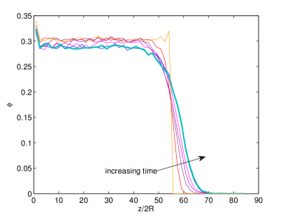
Figure 1: Interface formation for a fluidized bed of packing fraction $\bar{\phi}=0.3$. Time step in between two subsequent density profiles $\sim 20,50,100,200,400,400$ collisions per particle.

A simple model can account for the observed profiles and allows us to quantify the width of the interface. We consider a bed, extended to negative $z$, so that the probability to find particle $i$ at position $z$ in the homogeneous state is given by

$$p_{hom}(z)=p_{0}\theta(h-z)$$ (12)

At the interface, several processes disturb the particle position. We model these by a Gaussian with zero mean and variance $\sigma^{2}$. Hence the probability to find the particle at position $z$ is given by a convolution

$$p(z) = (p_{hom}\star p_{\sigma})(z)$$ (13)

$$= \frac{p_{0}}{2}\left(1-\textrm{erf}\left(\frac{z-h}{\sqrt{2}\sigma}\right)\right)\,.$$

The packing fraction is proportional to this probability and the proportionality constant can be fixed by requiring $\phi=\bar{\phi}$ well inisde the bulk

$$\phi(z)=\frac{\bar{\phi}}{2}\left(\textrm{erfc}\left(\frac{z-h}{\sqrt{2}\sigma}\right)\right)\,.$$ (14)

Hence we have two free parameters, we call $h$ the height of the bed and $\sigma$ is a measure for the sharpness of the interface: The smaller $\sigma$ the sharper the interface.

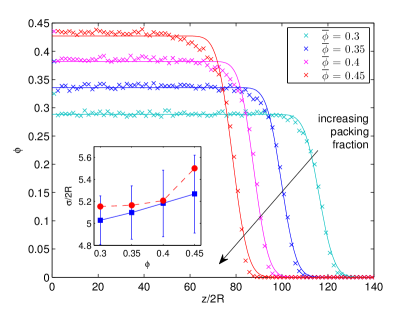
Figure 2: Packing fraction profiles for fluidized states of different flow rates, corresponding to stationary packing fractions $\bar{\phi}=0.3$. $0.35$, $0.4$ and $0.45$. Data points (crosses) are fitted (solid lines) to Eq. 14; inset: width of the interface as a function of average packing fraction $\bar{\phi}$ for two different values of $\Delta$.

We fit the packing fraction profile to Eq.(14) for fluidized states of several packing fractions. As discussed above, at the system bottom the packing fraction is locally increased. Therefore, we exclude these data points from the following procedure. The data and the resulting fits are plotted in Fig. 2. Our modeled packing fraction profile in Eq. (14) matches the measured data very well for moderately dense packings, but deviates for higher densities in the region where the bulk value starts to drop down. Nevertheless we can use the fit procedure to determine the width of the interface, which is shown in the inset of Fig. 2 as a function of packing fraction. The width of the interface $\sigma$ is in the range of $10$ particle radii and is approximately independent of $\phi$.

To calculate the local packing fraction we have used a slice of thickness $\Delta=10R$. We do not expect that the resolution in the local density has strong effects in the bulk of the sample. However the interface and in particular its width might depend on $\Delta$. To check this point we simulate the same fluidized bed but with a different value of $\Delta=6R$. The width of the interface $\sigma$ is compared for the two resolutions in the inset of Fig. 2. On average, $\sigma$ is slightly smaller for $\Delta=6R$. However the effect is small and we do not expect that a further refinement of the resolution for the density will change these results.

IV.2 Sedimentation and Expansion

So far we have shown that our simple model allows for a stationary state with a well defined interface whose width has been characterized. In this section we study the relaxational dynamics of the fluidization and sedimentation process which in experiment is achieved by changing the flow rate. The initial and final flow rate give rise to different stationary packing fractions. In our simple model sedimentation and compactification is modeled by a sudden (instantaneous) change in density. Specifically, we compact a fluidized bed with $N=10^{4}$ particles from $\bar{\phi}=0.3$ to a different packing fraction $\bar{\phi}=0.55$. The initial state is chosen as the stationary state for $\bar{\phi}=0.3$ and then at $t=0$ the average volume fraction is set to $\bar{\phi}=0.55$ in Eq.(9). To illustrate the sedimentation process, we depict the compactifying bed at six different times during the sedimentation in Fig. 3. Already from this figure, especially the second and third frame, one can see that the sedimentation process is not homogeneous.

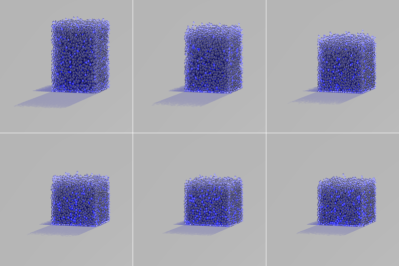
Figure 3: Sedimentation process from $\bar{\phi}=0.3$ to $\bar{\phi}=0.55$, at times $t=0,0.4,0.8,1.2,1.6,2.0s$. At the upper left, the bulk has a packing fraction $\approx 0.3$, at the lower right $\approx 0.55$, see also Fig. 4.

To quantify this process, we plot in Fig.4 the density profile for several intermediate time steps. The compactification starts from the bottom of the fluidized bed, working its way up to the top. The packing fraction starts to increase to the final value $\bar{\phi}=0.55$ at the bottom, subsequently the layers above are compacting and after about $500$ collisions per particle at $t=2s$ the new stationary state is attained.

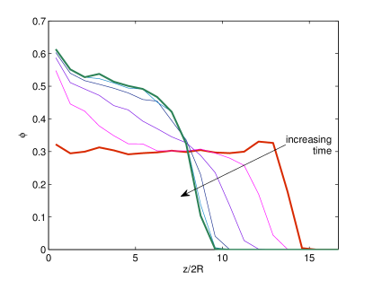
Figure 4: Packing fraction profiles for sedimentation from $\bar{\phi}=0.3$ to $\bar{\phi}=0.55$, time step $\Delta t=0.4s$. Same data as in Fig. 3.

Similarly, we monitor the reverse process, i.e. expansion of the bed. The initial state is chosen as the stationary state for $\bar{\phi}=0.55$ and then at $t=0$ the average volume fraction is set to $\bar{\phi}=0.3$ in Eq.(9). The density profile is shown in Fig.5 for several timesteps.

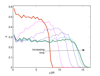
Figure 5: Expansion from $\bar{\phi}=0.55$ to $\bar{\phi}=0.3$, time step $\Delta t=0.16$.

The expansion process is inhomogeneous as well. The bed rapidly expands at the top with a simultaneous inhomogeneous dilution in the compactified region. Subsequently the upper part of the system continues to expand until the packing fraction has ultimately flattened throughout the system. The expansion process is faster than the sedimentation. After about $90$ collisions per particle at time $t=0.8s$ the bed has attained the expanded state.

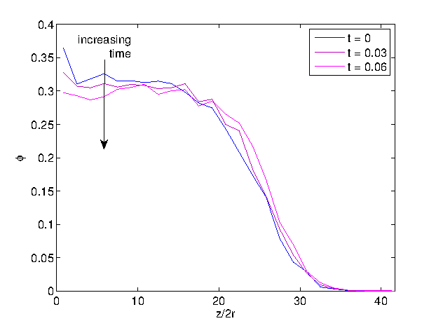
Figure 6: Expansion from $\bar{\phi}=0.35$ to $\bar{\phi}=0.3$.

The above expansion corresponds to a drop of almost $50\%$ in density and is by no means quasistatic. To study the latter, we consider a much smaller drop in density, from $\bar{\phi}=0.35\to 0.3$. The profiles are shown in Fig. 6 and observed to be approximately monotonic as a function of height within the bed.

We want to extract a timescale for the expansion and study its dependence on average packing fraction and coefficient of restitution. To that end we define the average deviation from the initial profile

$$L^{2}(t)=\int_{0}^{\infty}dz|\phi(z,t)-\phi(z,0)|^{2}$$ (15)

and compute its temporal evolution. As seen in Fig. 7, there is a rapid increase for short times followed by a plateau at longer times. The data are well fitted by an exponential increase according to: $L(t)=const.(1-e^{-\lambda t})$. In the inset of Fig. 7 we show $\lambda(\bar{\phi})$ as a function of average packing fraction for small changes of packing fraction, i.e. the first point corresponds to $\bar{\phi}=0.35$ to $\bar{\phi}=0.3$, the second point to $\bar{\phi}=0.4$ to $\bar{\phi}=0.35$ and so on. The timescale of expansion increases with increasing volume fraction and is slightly larger for the more inelastic systems.

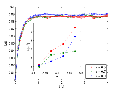
Figure 7: Approach to the stationary state, as measured by $L(t)$ for the expansion from $\bar{\phi}=0.35$ to $\bar{\phi}=0.3$; inset: $\lambda(\bar{\phi})$ for three different $\varepsilon$

V Conclusion and Outlook

We have shown how to simulate a fluidized bed with an event-driven method that is capable of simulating large numbers of particles. The algorithm is based on an expansion around the homogeneous fluidized state.

We found stable homogeneous fluidized beds, whose packing fraction can be adjusted by changing the flow rate. A stable bed is characterized by an interface at the top of the system, whose width is of the order of 5-10 particle radii. A stable bed also forms after changing the flow rate to a lower value, which increases the packing fraction (sedimentation), and by increasing the flow rate, which decreases the packing fraction (expansion). In general, the processes of sedimentation and expansion are non homogeneous, i.e. the packing fraction in the dense region does not deform homogeneously but rather changes from bottom to top, ultimately flattening to the previously observed stationary profiles.

We plan to further investigate fluidized beds using our algorithm. An obvious first extension is the temperature profile. Furthermore, we can easily compute velocity distributions and mean square displacements, which are also accessible to experiment by introducing markers.

Here, we have focused on approximately homogeneous states. However, it is known Guazelli and Hinch (2011) that suspensions of sedimenting particles exhibit a rich spectrum of instabilities. We have already seen striped phases in our simulations for very small noise levels, but postpone a sytematic study to future work.