Probing baryonic processes and gastrophysics in the formation of the Milky Way dwarf satellites: I. metallicity distribution properties

Abstract

The Milky Way (MW) dwarf satellites, as the smallest galaxies discovered in the present-day universe, are potentially powerful probes to various baryonic processes in galaxy formation occurred in the early universe. In this paper, we study the chemical properties of the stars in the dwarf satellites around the MW-like host galaxies, and explore the possible effects of several baryonic processes, including supernova (SN) feedback, the reionization of the universe and H₂ cooling, on them and how current and future observations may put some constraints on these processes. We use a semi-analytical model to generate MW-like galaxies, for which a fiducial model can reproduce the luminosity function and the stellar metallicity–stellar mass correlation of the MW dwarfs. Using the simulated MW-like galaxies, we focus on investigating three metallicity properties of their dwarfs: the stellar metallicity–stellar mass correlation of the dwarf population, and the metal-poor and metal-rich tails of the stellar metallicity distribution in individual dwarfs. We find that (1) the slope of the stellar metallicity–stellar mass correlation is sensitive to the SN feedback strength and the reionization epoch; (2) the extension of the metal-rich tails is mainly sensitive to the SN feedback strength; (3) the extension of the metal-poor tails is mainly sensitive to the reionization epoch; (4) none of the three chemical properties are sensitive to the H₂ cooling process; and (5) comparison of our model results with the current observational slope of the stellar metallicity–stellar mass relation suggests that the local universe is reionized earlier than the cosmic average and local sources may have a significant contribution to the reionization in the local region, and an intermediate to strong SN feedback strength is preferred. Future observations of metal-rich and metal-poor tails of stellar metallicity distributions will put further constraints on the SN feedback and the reionization processes.

1. Introduction

The dwarf satellite galaxies around the Milky Way (MW), including both classical dwarf spheroidal galaxies (dSphs) and ultra-faint dwarf galaxies, are among the least massive galaxies found in the universe (e.g., Zucker et al., 2006; Martin et al., 2007; Strigari et al., 2008; Geha et al., 2009; Simon et al., 2011; McConnachie, 2012). They are believed to form at early times of the cosmic history and reside in small dark matter sub-halos with shallow gravitational potentials (e.g., Macciò et al., 2010; Koposov et al., 2008, 2009). They are one of the most representative classes of objects for studying the effects of various baryonic processes involved in galaxy formation and in the early universe, such as supernova (SN) feedback (see Font et al., 2011; Wyithe & Loeb, 2013; Robertson et al., 2005), the reionization of the universe (e.g., Bullock et al., 2000; Somerville, 2002; Benson et al., 2002; Grebel & Gallagher, 2004; Wyithe & Loeb, 2006; Bovill & Ricotti, 2009; Muñoz et al., 2009; Busha et al., 2010; Lunnan et al., 2012), and molecular hydrogen cooling (e.g., Benson 2010). Understanding these processes is one important step to understand the problems that the $\Lambda{\rm CDM}$ cosmology faces at small galactic scales, such as, the ‘missing satellite problem’ (Klypin et al., 1999; Moore et al., 1999; Kravtsov et al., 2004; Strigari et al., 2007; Simon & Geha, 2007; Brooks et al., 2013) and the ‘core/cusp problem’ (e.g. see de Blok 2010 and the references therein). In this paper, we study the chemical properties of the stars in the dwarf satellites around the MW-like host galaxies, and explore the possible effects of the above baryonic processes on them and how current and future observations may put some constraints on these processes.

The chemical properties of the dwarfs are potentially powerful probes of the above baryonic processes (e.g., Font et al. 2011; Frebel et al. 2010). The chemical enrichment of a galaxy are connected directly with the SN feedback process and the star formation history. The heavy elements were first synthesized by nuclear reactions in stars and can be ejected into the interstellar medium at the later stages of stellar evolution, through stellar winds and SN explosion; and some chemical-enriched interstellar medium can in turn participate in the later formation of stars with enhanced metal abundance (see Benson, 2010, for a review). The processes may occur repeatedly over time along the star formation history. Different from the present-day star formation, the star formation in the early universe can be affected significantly by the reionization of the universe and the molecular hydrogen cooling processes: the molecular hydrogen cooling was proposed to be an important cooling mechanism in forming first stars/galaxies in metal-free mini-halos in the early universe, where the gas temperature of the mini-halos is not high enough to have effective atomic cooling (e.g., Bromm 2013, Abel et al. 2002, Bromm et al. 2002); and the reionization of the universe may result in gas heating-up with increasing pressure and the photoevaporation of small gaseous halos and hence suppress star formation (e.g., Gnedin, 2000; Kravtsov et al., 2004; Okamoto et al., 2008).

In this paper, we employ the dark matter halo merger trees and the semi-analytical galaxy formation model (Cole et al., 2000, see also White & Frenk 1991; Kauffmann et al. 1993; Somerville & Primack 1999) to generate the MW-like galaxies and their dwarf satellites. The model, with preferred model parameters, can reproduce the luminosity function of the dwarf satellites, the observed metallicity versus luminosity/stellar mass correlation of the dwarf population, and also the stellar metallicity distribution of some individual dwarfs. Armed with this model, we further explore the effects of various baryonic processes on the metallicity properties by choosing different recipes for those processes. By comparing the model results with the observational metallicity properties of dwarf satellites, we investigate the possibility of using the metallicity properties to constrain the baryonic processes, such as the supernova feedback, the reionization of the universe, and the molecular cooling, involving in the formation processes of those satellites.

The observational metallicity properties have recently been used to understand the origin of the dwarfs and constrain their formation histories. For example, Kirby et al. (2011a, b) use the metallicity distributions of eight MW classical dSphs to constrain their star formation histories, as well as the chemical enrichment mode, i.e., the roles of inflow and outflow in the enrichment histories; and Salvadori & Ferrara (2009) use the stellar metallicity–luminosity correlation and the mean metallicity distribution of ultra-faint dwarfs to understand their formation sites, redshifts, and star formation histories. Our study is distinguished from previous works in a few aspects of the purpose and the method details as follows.

• We consider the detailed assembling history and the accompanied star formation history of each dwarf satellite through a semi-analytical modeling of the MW formation. Many previous works adopt simple description of the star formation history for individual dwarfs (e.g., Carigi et al., 2002; Lanfranchi & Matteucci, 2003, 2004; Fenner et al., 2006; Marcolini et al., 2006, 2008; Kirby et al., 2011b), which does not include the detailed assembling history of galaxies and their dark matter halos.

• The chemical enrichment caused by SNe II and Ia are different in the time delay of ejecting enriched materials after the star formation and in the element abundance of ejected materials (e.g., Matteucci & Recchi, 2001). We consider the time delay of the SN Ia enrichment after star formation explicitly in the chemical enrichment model; while a number of previous works only use simple instantaneous recycling of ejected materials, which may not address the SN Ia enrichment properly (e.g., Lanfranchi & Matteucci, 2004). We note that the chemical enrichment of SNe Ia has been considered in some semi-analytical galaxy formation model (e.g., Nagashima et al. 2005a, b; Yates et al. 2013), for example, for intracluster medium, elliptical galaxies, or MW-like disk galaxies, but not for galaxies as small as the the dwarfs around the MW.

• We quantify the extension of the metal-poor and metal-rich tails in the stellar metallicity distribution and explore the possibility to use them as a probe of the baryonic processes.

• The semi-analytical galaxy formation models have also been used to explore some properties of the dwarfs (e.g., Font et al. 2011; Guo et al. 2011; Li et al. 2010; Romano & Starkenburg 2013); however, those previous studies focus mainly on different aspects, e.g., on the number abundance of the dwarfs or the chemical evolution in an individual (Sculptor) dwarf. Font et al. (2011) illustrate that the chemical properties of the dwarfs can be used to break the degeneracy in the effects of SN feedback and reionization on their luminosity function.

• In addition, we adopt the Monte-Carlo method based on the modified extended Press-Schechter function to generate dark matter halo merger trees. By this method, a large number of trees (e.g., 100 or more trees) can be generated for each set of parameters in an efficient way, which allows a statistical study of the dwarf chemical properties. Numerical simulations have provided the assembly histories of several MW-sized halos, e.g., the Via Lactea simulation (Diemand et al., 2007; Rocha et al., 2012) and the Aquarius simulation (Springel et al., 2008; Starkenburg et al., 2013); however, a much larger number of merger trees for MW-sized halos directly from numerical simulation are still not available.

The paper is organized as follows. The semi-analytical galaxy formation model used in this study is described briefly in Section 2, with emphases on the recipes of the SN feedback and the SN Ia explosion rate that implemented. We use the model to generate the MW-like galaxies and their dwarfs in Section 3. The model with a set preferred parameters can reproduce the observational results on the metallicity properties of the MW dwarf satellites well. We also show the obtained stellar metallicity versus stellar mass correlation and the metallicity distribution of the dwarfs, by using different recipes for SN feedback, reionization of the universe, and molecular hydrogen cooling. Note that in this paper the metallicity is expressed through [Fe/H], and we do not consider the detailed distribution of alpha and other elements. The constraints on the various physical processes are discussed in Section 4, and conclusion is given in Section 5.

We note that the age properties of the dwarf satellites can be also used to put constraints on the above several baryonic processes, in addition to the chemical properties investigated in this paper. We shall adopt a similar method to explore the constraints from the age properties in a subsequent paper (in preparation).

In this paper we set the Hubble constant as $H_{0}=100\,h{\rm\,km\,s^{-1}}{\rm\,Mpc}$, and the cosmological model used is $(\Omega_{\rm m},\Omega_{\Lambda},h,\sigma_{8})=(0.25,0.75,0.70,0.90)$.

2. Method

In this section, we briefly describe the semi-analytical galaxy formation model that is used to explore the metallicity properties of the MW satellites. The backbone of the model is the merger trees of MW-sized dark matter halos, which may represent the hierarchical growth history of the MW host halo. Detailed semi-analytical recipes for galaxy formation and evolution (for references, see Cole et al., 2000; White & Frenk, 1991; Kauffmann et al., 1993; Somerville & Primack, 1999) are incorporated into the merger trees to obtain the observational properties of the central MW galaxy and its satellites.

We plant the merger trees of MW-sized halos by the Monte-Carlo method developed by Parkinson et al. (2008, see also ), which is based on a modified version of the extended Press-Schechter formula. The obtained halo mass functions are in good agreement with the N-body simulation results. The merger trees are built from redshift $z=0$ to $20$, with 79 equal intervals in the logarithm of $1+z$. The mass resolution of the merger trees is set to be $1.0\times 10^{6}{\,M_{\odot}}$ , which is the typical mass of mini-halos that may be important for primordial star formation at high redshift $z\sim 20$. According to the current constraints on the MW halo mass (e.g., Boylan-Kolchin et al. 2013 and references therein), i.e., $1-2\times 10^{12}{\,M_{\odot}}$, we obtain the merger trees for halos with the present-day mass $M_{\rm halo}$ of $1.0\times 10^{12}$ and $2.0\times 10^{12}{\,M_{\odot}}$, respectively.

The semi-analytical galaxy formation model in this study is based on GALFORM (Cole et al., 2000; Benson et al., 2003; Bower et al., 2006), but with several modifications. As demonstrated by Cole et al. (2000), Kauffmann et al. (1993), Somerville & Primack (1999), Croton et al. (2006), and Bower et al. (2006), the semi-analytical models can successfully reproduce a number of observations on the statistical distributions of galaxy properties, including the galaxy luminosity function, the stellar mass function, etc. Some constraints on the parameters involving in the semi-analytical model have been obtained by using those observations; however, there are still large degeneracies among those parameters as suggested by recent studies exploring the parameter space of the semi-analytical galaxy formation model (e.g., Lu et al., 2011, 2012; Bower et al., 2010). The metallicity properties studied in our study may also put some constraints on the model parameters, especially those characterized SN feedback, the reionization of the universe, molecular cooling in the early universe. We vary the model parameters involving in these several processes to check the effects of those parameters on the metallicity properties of the MW dwarfs.

The related recipes, e.g., on SN feedback, reionization, and molecular hydrogen cooling, are summarized below. For each set of the recipe parameters, we generate $100$ merger trees and apply the semi-analytical recipes to them. The various related baryonic processes (e.g., star formation, chemical enrichment, and galaxy mergers) are calculated in a time step $\Delta t\sim 10^{6}{\rm yr}$. From the obtained present-day galaxies, we select the MW-like hosts for the study of their satellites. The MW-like hosts are selected by the criteria that the total stellar mass of a present-day host galaxy is in the range of $4\--6\times 10^{10}{\,M_{\odot}}$ and its bulge mass-to-disk mass ratio is between $0.1$ and $0.4$. Along the assembling history of the MW-sized halo, a satellite of the present-day MW galaxy was a host galaxy of a small halo at an early time before it fell into a big halo. An example of the dwarf satellite luminosity function obtained from our models is illustrated in Figure 1.

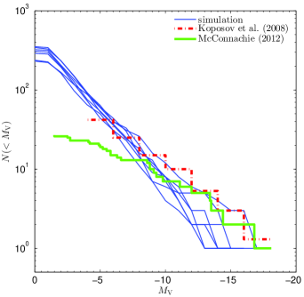
Figure 1.— An example of the cumulative luminosity functions of the dwarf satellites of the MW-like galaxies obtained from our models. The $y$-axis represent the number of the satellites with absolute magnitude brighter than $M_{V}$. The seven blue solid lines are the simulation results of the first parameter set listed in Table LABEL:tab:parameter_sets, and each line is for one MW-like host galaxy. The green line shows the observational result for 27 MW satellites (McConnachie, 2012), and the red one is the result after doing the searching volume correction (Koposov et al. 2008; see also Tollerud et al. 2008). Our simulation results generally reproduce the observational luminosity function of the MW dwarf satellites.

As seen from Table LABEL:tab:parameter_sets to be listed in Section 3 below, for some recipe parameter sets, the models fail to generate the MW-like host galaxy. In these cases, we just choose randomly $10$ results of the corresponding parameter set to illustrate the effects of the baryonic processes.

• The reionization of the universe: the reionization in the early universe reduces the baryon fraction of a dark matter halo. During the reionization epoch, the intergalactic medium (IGM) heats up with increasing pressure, which can suppress the collapse of the IGM onto dark matter halos, and the gas that was previously in a dark matter halo can also evaporate out of the halo. The extent of the reduction in the baryon fraction of a dark matter halo depends on the halo gravitational potential or roughly the halo mass. The dependence is modeled through a mass scale called the ‘filtering mass’ ($M_{\rm F}$) as follows,

  $$f_{\rm b}=\frac{1}{[1+(2^{1/3}-1)M_{\rm F}/M_{\rm halo}]^{3}}$$ (1)

  where $f_{\rm b}$ is the ratio of the baryon fraction in a halo with mass $M_{\rm halo}$ to the cosmic average baryon fraction, and $M_{\rm F}$ is a function of redshift, as well as a function of the completion redshift and the duration of the reionization process. A halo with mass $M_{\rm halo}<M_{\rm F}$ loses more than 50% of baryonic matter expected by the cosmic average. In this paper, we use Equations (B1) and (B2) in Kravtsov et al. (2004) (see also Gnedin 2000; Okamoto et al. 2008) to calculate $M_{\rm F}$ and model the effects of the reionization. This reionization recipe for $M_{\rm F}$ is characterized by two parameters: $z_{0}$, the redshift that the first ionized bubble formed, and $z_{\rm r}$, the completion redshift of the reionization.

  Two sets of the reionization parameters are used in our model, i.e., $(z_{0},z_{\rm r})=(15,10)$ and $(10,7)$. Observations on the highest redshift QSOs suggest that the reionization process is completed at redshift $z\sim 6-7$ (e.g., Becker et al. 2001; Mortlock et al. 2011), and the polarized cosmic microwave background radiation detected by WMAP and PLANCK suggests that the universe probably began to be reionized at redshift $z\gtrsim 10$ (e.g., Hinshaw et al., 2013; Planck Collaboration et al., 2013). According to these observations, the reionization model set by $(z_{0},z_{\rm r})=(10,7)$, suggested by Kravtsov et al. (2004), may represent a case close to or slightly later than the cosmic average reionization epoch of the real universe, and the other model set by $(z_{0},z_{\rm r})=(15,10)$ may represent a case a little earlier than the cosmic average of the real universe. Hereafter, we refer the former case as ‘weak reionization’ (or ‘late reionization’) and the latter case as ‘strong reionization’ (or ‘early reionization’). Note that Font et al. (2011) also adopt $(z_{0},z_{\rm r})=(15,10)$ as a ‘strong reionization’ scenario and suggest that the contribution from local sources may lead to an earlier reionization of the local patch compared with the cosmic average.

• Molecular hydrogen cooling: we model the molecular hydrogen cooling process occurred in the early universe by using Equations (21)–(29) in Benson (2010) (see also Galli & Palla 1998) and we do not allow any molecular hydrogen cooling after the completeness of the reionization, because the abundance of hydrogen molecules would be significantly suppressed by the strong UV background.

• Cooling of hot halo gas: The gas cooling recipe of the GALFORM is modified in this work. The cooling recipe in Cole et al. (2000) is likely to underestimate the amount of cooling gas in a halo, where the gas reheated by SNe is assumed not to participate into the cooling process until the dark matter halo doubles its mass along the merger trees. The cooling recipe in Bower et al. (2006) improves this but possibly overestimates the amount of cooling, and this model has to adopt an extremely strong SN feedback (e.g., $v{{}_{\rm hot}}=485{\rm\,km\,s^{-1}}$ and $\alpha{{}_{\rm hot}}=3.2$ in Eq. 3 below) to balance the overestimated cooling amount and reproduce the observational galaxy luminosity function. Benson & Bower (2010) further modify the cooling recipe by continuously updating estimate of cooling time and halo properties at each timestep. The model result of this update can match the observational galaxy luminosity function, but the gas phase metallicity is underestimated for relatively low-luminosity galaxies, where SN feedback is argued to be the main driver for the relation between the galaxy luminosity and the gas phase metallicity and the adopted strength is still high (with $v{{}_{\rm hot}}\sim 328$ or $358{\rm\,km\,s^{-1}}$ and $\alpha{{}_{\rm hot}}=3.36$; see Table 5 therein); and thus the cooling rate is likely to be still overestimated. In this work, we employ a cooling recipe somewhat between the recipes in Cole et al. (2000) and Bower et al. (2006). This modified recipe is detailed in the Appendix.

• SN feedback efficiency: SN feedback reheats the cold gas in a galaxy, expels it out of the galaxy, and enriches the metallicity in the halo gas. Following Cole et al. (2000), we use the formula

  $$dM_{\rm reheat}\ =\ \beta\psi dt$$ (2)

  $$\beta\ =\ (v_{\rm disk}/v_{\rm hot})^{-\alpha_{\rm hot}}$$ (3)

  to estimate the amount of cold gas expelled from a galaxy by SNe II, where $dM_{\rm reheat}$ is the mass of the gas reheated by SN feedback during time interval $dt$, $\psi$ is the star formation rate, $\beta$ is the SN feedback efficiency, $v_{\rm disk}$ is the circular velocity of the galaxy disk, and $\alpha_{\rm hot}$ and $v_{\rm hot}$ are two parameters defining the strength of the feedback. We call Equation (3) the SN feedback efficiency scaling law.

  Once the SN explosion energy is sufficiently high, all the reheated gas may be expelled out of the galaxy if the following energy condition is satisfied, i.e.,

  $$dE_{\rm SN}-\frac{1}{2}v_{\rm vir}^{2}dM_{\rm reheat}\geq 0,$$ (4)

  where $dE_{\rm SN}=\epsilon_{\rm halo}\times\frac{1}{2}v_{\rm SN}^{2}\psi dt$ is the total energy released by SNe II and coupling to the IGM during time $dt$, $v_{\rm vir}$ is the virial velocity of the halo, $\frac{1}{2}v_{\rm SN}^{2}$ is the total energy released per unit mass by SNe with $v_{\rm SN}=630{\rm\,km\,s^{-1}}$ for the Chabrier IMF (Chabrier, 2003), and $\epsilon_{\rm halo}=0.05$ is the fraction of the energy that couples to the cold gas in the disk (e.g., Li et al. 2010). If the energy condition (Inequality 4) is satisfied, the reheated gas can either be ejected into the dark matter halo or even escape out of the halo, with masses approximated by

  $$dM_{\rm outflow}$$ (5)

  $$= \min\left(\frac{dE_{\rm SN}-\frac{1}{2}v_{\rm vir}^{2}dM_{\rm reheat}}{\frac{1}{2}v_{\rm vir}^{2}},dM_{\rm reheat}\right),$$

  and

  $$dM_{\rm stay}=dM_{\rm reheat}-dM_{\rm outflow},$$ (6)

  where $dM_{\rm outflow}$ is the mass of the gas running out of the halo during time $dt$ and $dM_{\rm stay}$ is the mass of the reheated gas staying in the halo. We assume that the outflow returns to the halo on a halo dynamical time scale ($\tau_{\rm halo}\equiv r_{\rm vir}/v_{\rm vir}$, where $r_{\rm vir}$ is the halo virial radius) as

  $$dM_{\rm back}=\frac{M_{\rm outflow}}{\tau_{\rm halo}}dt.$$ (7)

  If the supernova explosion is energetic enough to expel all the reheated gas out of the dark matter halo, i.e., $(dE_{\rm SN}-\frac{1}{2}v_{\rm vir}^{2}dM_{\rm reheat})/(\frac{1}{2}v_{\rm vir}^{2})>dM_{\rm reheat}$ in Equation (5), Equations (5) and (6) reduce to

  $$dM_{\rm outflow}=dM_{\rm reheat},$$ (8)

  $$dM_{\rm stay}=0.$$ (9)

  If the energy condition is not satisfied, we use

  $$dM_{\rm outflow}=0,$$ (10)

  $$dM_{\rm stay}=dE_{\rm SN}/(\frac{1}{2}v_{\rm vir}^{2}),$$ (11)

  to determine the masses of the gas that goes out of the halo and stays in the halo, which is equivalent to replace the SN feedback scaling law with

  $$\beta=\beta_{E} \equiv dE_{\rm SN}/(\frac{1}{2}v_{\rm vir}^{2}\psi dt)=\epsilon_{\rm halo}(v_{\rm vir}/v_{\rm SN})^{-2}$$ (12)

  in Equation (2) above. Equation (12) represents the supernova feedback efficiency limit set by the energy condition.

  Figure 2 shows the relation between the SN feedback efficiency given by the scaling law and the limit set by the energy condition. The solid lines with different symbols show the feedback efficiency given by the scaling law with different values of $v_{\rm hot}$ and $\alpha_{\rm hot}$. Specifically, the solid line without symbols indicates the efficiency for the fiducial model ($v_{\rm hot}=200{\rm\,km\,s^{-1}}$ and $\alpha_{\rm hot}$=3.2, see the fiducial model defined below in Section 3). The dashed line gives the SN feedback efficiency limit set by the energy condition (Inequality 4); and the feedback efficiency is allowed by the energy condition in the region below the dashed line, while not allowed in the shaded region above. In the shaded region, Equations (10) and (11) are applied. The dotted line indicates the efficiency below which all the reheated gas is ejected out of the halo, where Equations (8) and (9) are applied. The dashed and the dotted lines are drawn under the assumption $v_{\rm vir}=v_{\rm disk}$, and the deviation from the assumption is somewhat significant only at low velocities. The region between the dotted line and the dashed line have $dM_{\rm outflow}>0$ and $dM_{\rm stay}>0$, described by Equations (5) and (6).

  

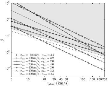
  Figure 2.— The SN feedback efficiency $\beta$ given by the feedback scaling law as a function of $v_{\rm disk}$ and the limit set by the energy condition. The solid lines represent the feedback scaling laws with different values of $v_{\rm hot}$ and $\alpha_{\rm hot}$, and specifically, the solid line without symbols is for the fiducial model with $v_{\rm hot}=200{\rm\,km\,s^{-1}}$ and $\alpha_{\rm hot}=3.2$. The dashed line represents the limit set by the energy condition. The feedback efficiency $\beta$ (Eq. 3) is allowed by the energy condition in the region below the dashed line, while not allowed in the gray shaded region above it. The dotted line indicates the feedback efficiency below which all the reheated gas would be ejected out of the halo. The dashed and the dotted lines are drawn under the assumption $v_{\rm disk}=v_{\rm vir}$, which is a plausible assumption in general; and the efficiency limits may scatter around the lines due to the scatter of $v_{\rm vir}$ around $v_{\rm disk}$.

  As mentioned before, along the assembling history of the MW-like halo, a satellite of the present-day MW may be a host galaxy of a small isolated halo before it falls into a big halo at an early time. We apply the above energy condition only to a galaxy before it becomes a satellite. We do not apply it to satellites, but assume that the reheated gas from satellites (with mass expected by Eqs. 2 and 3) is expelled into the big host halo, as the original halos of the satellites are largely tidally disrupted along their motion in the big host halo, and the tidal field induced by the big host halo also helps to keep those expelled materials out of the satellites.

• Metallicity production: In this work, the Fe yield of SNe II is adopted from tables 2–3 in Nomoto et al. (2006), and the Fe yield of SNe Ia is from Iwamoto et al. (1999). The metals ejected by SNe are assumed to be homogeneously and instantaneously mixed with the interstellar medium in the galaxy; and after the mixture, some metals can be ejected out of the galaxy along with the mixed interstellar medium that is ejected out by SN explosions.

• Chemical enrichment due to SN Ia explosions: The feedback due to SN Ia explosions is explicitly included in this work. We assume that the energy released by a SN II explosion and a SN Ia explosion is the same. We use the same feedback recipe for them (Eqs. 2–11), but include the non-negligible time delay between the formation of SN Ia progenitors and the SN Ia explosions. In the model, the number of SN Ia explosions within a time interval $\Delta t$ which begins at a given time $t$, denoted by $N_{\rm Ia}(t)$, is given by

  $$N_{\rm Ia}(t) = \int_{t}^{t+\Delta t}dt^{\prime\prime}\int_{0}^{t^{\prime\prime}}R_{\rm Ia}(t^{\prime\prime}-t^{\prime})\psi(t^{\prime})dt^{\prime},$$ (13)

  $$\simeq \Delta t\times\int_{0}^{t}R_{\rm Ia}(t-t^{\prime})\psi(t^{\prime})dt^{\prime},$$

  where $t^{\prime\prime}-t^{\prime}$ is the stellar population age, $R_{\rm Ia}$ is the SN Ia explosion rate as a function of the time delay and in units of number per time per mass (e.g., ${\rm\,Gyr}^{-1}{\,M_{\odot}}^{-1}$), and $\Delta t\sim 10^{6}{\rm\,yr}$ is small enough compared to the time delay of SNe Ia explosion assumed below. According to the observational SN Ia rate $R_{\rm Ia}$ reported by Maoz et al. (2010), a time delay of $0.1{\rm\,Gyr}$ is assumed to generate SN Ia since the formation of a stellar population, and the number of the generated SNe decreases with increasing age of this population as a power law. Nagashima et al. (2005a, b) also considered the chemical enrichment due to SN Ia explosions in their semi-analytical galaxy formation model, where the star formation history of a galaxy is re-binned into $30$ rough time bins to obtain the convolution integral of Equation (13). In this work, we still use the star formation history obtained with small timesteps $\Delta t$, but approximate the power-law decline of the SN Ia explosion rate as a combination of the linear functions and the exponential function, which can expedite the calculation of the convolution integral and obtain $N_{\rm Ia}(t)$ recursively and efficiently in each timestep. The method to calculate the SN Ia explosion rate is detailed below.

  We approximate the power-law rate into $6$ continuous linear segments when the stellar population age $\tau$ is between $0.1$ and $2{\rm\,Gyr}$. The $i$-th segment approximates the power-law rate when $\tau$ is from $\tau_{i-1}$ to $\tau_{i}$ ($i=1,2,...,6$), with $\tau_{0}=0.1{\rm\,Gyr}$ and $\tau_{6}=2{\rm\,Gyr}$. When the stellar population age is older than $2{\rm\,Gyr}$, we approximate the power-law rate by an exponential tail $C_{\rm Ia}\exp(c_{0}t^{\prime})$, where $C_{\rm Ia}$ is a normalization factor and $c_{0}$ is a parameter, and we adopt $C_{\rm Ia}=5\times 10^{-4}{\rm\,Gyr}^{-1}{\,M_{\odot}}^{-1}$. Note that Maoz et al. (2010) report $C_{\rm Ia}=1\times 10^{-3}{\rm\,Gyr}^{-1}{\,M_{\odot}}^{-1}$, and Kirby et al. (2011b) mention that the observations in Maoz et al. (2010) can easily be consistent with half of that value. The parameter $c_{0}$ is fixed by requiring the exponential tail and the sixth segment give the same value at $\tau=2{\rm Gyr}$. The relative error in $R_{\rm Ia}$ caused by the approximation described above is about 0.15%. With the approximation, we have the following recursive formulas for $N_{\rm Ia}$, with which the computational complexity is significantly reduced,

  $$N_{\rm Ia}(t+\Delta t) = N_{\rm Ia}(t)+\sum_{i=1}^{6}k_{i}\Delta t^{2}M_{i}(t+\Delta t)$$

  $$+ (k_{1}\tau_{0}+b_{1})\psi(t-\tau_{0}+\Delta t)\Delta t^{2}$$

  $$+ N_{\rm exp}(t+\Delta t)-N_{\rm exp}(t),$$

  where $k_{i}$ and $b_{i}$ are the slope and intercept of the $i$-th linear segment of the approximated SN Ia explosion rate, respectively, and

  $$M_{i}(t+\Delta t) = M_{i}(t)-\psi(t-\tau_{i}+\Delta t)\Delta t$$ (15)

  $$+\psi(t-\tau_{i-1}+\Delta t)\Delta t,$$

  $$N_{\rm exp}(t+\Delta t) = N_{\rm exp}(t)\exp(c_{0}\Delta t)$$

  $$+\psi(t-\tau_{6}+\Delta t)C_{\rm Ia}\exp(c_{0}\tau_{6})\Delta t^{2},$$

  $$M_{i}(0) = 0,$$

  $$N_{\rm exp}(0) = 0,$$

  are used to define and calculate $M_{i}$ ($i=1,2,...,6$) and $N_{\rm exp}$.

Note that tidal disruption of the original halo of a satellite after its infalling into a big host halo is included when considering the effect of SN feedback, as mentioned above; but we ignore the tidal stripping and disruption of its stellar and cold gas components in our model. Compared with the original halo size of the satellite, the stellar and cold gas components are located in a smaller central region of the halo, which should be affected less by tidal effects from the big host halo. In addition, Starkenburg et al. (2013) show that the tidal stripping and disruption of satellites have a small effect on the satellite total luminosity function.

3. Results

In this section, we try different recipe parameters for the processes of the supernova feedback, the reionization of the universe, and the molecular hydrogen cooling. The different sets of the parameters are listed in Table LABEL:tab:parameter_sets. We find one set of parameters that can reproduce some observational properties of the MW dwarfs better than the others, including the satellite luminosity function, their luminosity/stellar mass versus stellar metallicity correlation, and the metallicity distributions of the classical dSphs, as well as the host galaxy properties (stellar mass, bulge-to-disk mass ratio); and we denote the model with this set of parameters by ‘the fiducial model’ and list it as the first parameter set in Table LABEL:tab:parameter_sets. Comparison of the results obtained with the other different parameter sets helps us to investigate the effects of the physical processes. We present our model results on the stellar mass versus stellar metallicity correlations of the dwarfs in Section 3.1 and the stellar metallicity distribution in individual dwarfs in Section 3.2.

Table 1The parameter sets used in the paper

$v_{\rm hot}({{\rm\,km\,s^{-1}}})$	$\alpha_{\rm hot}$	$z_{0}$	$z_{\rm r}$	$M_{\rm halo}({\,M_{\odot}})$	${\rm H}_{2}$ cooling	MW-like galaxies
$200$	$3.2$	$15$	$10$	$2\times 10^{12}$	on	$7$
$400$	$3.2$	$15$	$10$	$2\times 10^{12}$	on	0
$100$	$3.2$	$15$	$10$		on	0
$50$	$3.2$	$15$	$10$		on	0
$200$	$4.0$	$15$	$10$		on	$9$
$200$	$2.0$	$15$	$10$		on	$18$
$200$	$3.2$	$10$	$7$		on	$8$
$200$	$3.2$	$15$	$10$		off	$9$
$400$	$3.2$	$15$	$10$	$1\times 10^{12}$	on	0
$100$	$3.2$	$15$	$10$		on	$12$
$50$	$3.2$	$15$	$10$		on	$13$
$200$	$4.0$	$15$	$10$		on	$9$
$200$	$2.0$	$15$	$10$		on	$10$
$200$	$3.2$	$10$	$7$		on	$17$
$200$	$3.2$	$15$	$10$		off	$7$

We find that the chemical properties of the satellites obtained from $M_{\rm halo}=1\times 10^{12}$ and $2\times 10^{12}{\,M_{\odot}}$ do not differ much, so below we only show the results of $M_{\rm halo}=2\times 10^{12}{\,M_{\odot}}$ for brevity.

3.1. The stellar mass – metallicity correlation

Figure 3 shows the stellar metallicity versus luminosity correlation of the dwarfs generated by the fiducial model, as well as the observational results (Kirby et al., 2011a; Martin et al., 2008; Helmi et al., 2006; van den Bergh, 2000). As seen from Table LABEL:tab:parameter_sets, 7 individual simulations can generate a MW-like host galaxy, and the first $7$ panels in Figure 3 show each result of the individual simulations. The last panel shows the results of these simulations together. In each of the first seven panels, the red line shows the best fit to the simulation results by using the least squares method; $\alpha$ is the best-fit slope, and $b_{\rm[Fe/H]}$ is the best-fit intercept at $\log(L_{\rm V}/L_{{\rm V},\odot})=0$. The red line in the last panel shows the statistical average of the best-fits in the first 7 panels, and the parameters labeled represent the statistical mean and standard deviation of the 7 best-fit slopes and intercepts. The fiducial model reproduces the observations well. While the stellar metallicity – luminosity correlation is convenient for comparison with observations, in this work we use the stellar mass – metallicity correlation of the dwarfs obtained from simulations to study the effects of supernova feedback, reionization, and molecular hydrogen cooling, as the physical processes affect the star formation histories of the dwarfs directly. The faintest satellite in the observation sample shown in Figure 3 has $\log(L_{\rm V}/L_{{\rm V},\odot})=3.6\pm 0.2$, and in our simulations the satellites with this luminosity roughly have stellar masses $\sim 10^{4}{\,M_{\odot}}$. Thus in our study of the stellar mass – metallicity correlations below, we adopt $10^{4}{\,M_{\odot}}$ as the cut-off mass at the low-mass end of the satellites.

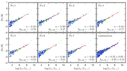
Figure 3.— The stellar metallicity – luminosity correlations of the satellites of the MW-like galaxies. In the first seven panels, the blue dots represent the satellites from the simulations. The green dots and their error bars are the data from the observations (Kirby et al. 2011a for Fornax, Leo I, Sculptor, Leo II, Sextans, Draco, CVn I, Ursa Minor, Leo T, Hercules, Ursa Major I, Leo IV, CVn II, Ursa Major II, ComB, and Martin et al. 2008 for Bootes I, Helmi et al. 2006 for Carina, and van den Bergh 2000 for the Large Magellanic Cloud and the Small Magellanic Cloud). In the first seven panels, the red lines are the best linear fits to the simulations, where $\alpha$ is the best fit slope and $b_{\rm[Fe/H]}$ is the best-fit intercept at $\log(L_{\rm V}/L_{{\rm V},\odot})=0$; and that in the last panel shows the statistical average of the results shown in the first seven panels. The parameters labeled in the last panel represent the statistical mean and standard deviation of the seven best-fit slopes and intercepts.

We show the dependence of the stellar mass – metallicity correlation on the SN feedback parameters, the reionization, and molecular hydrogen cooling below in Sections 3.1.1–3.1.3.

3.1.1 Dependence on SN feedback

We study the dependence of the stellar mass – stellar metallicity correlation on SN feedback through its dependence on the parameters ($v_{\rm hot},\alpha_{\rm hot}$).

Figure 4 shows the stellar mass – stellar metallicity correlations obtained from the models with different values of $v_{\rm hot}$ in different panels. Each panel shows the combined results of the corresponding simulations together, as the last panel of Figure 3 does. As seen from Figure 4, the models with $v_{\rm hot}=200{\rm\,km\,s^{-1}}$ and $v_{\rm hot}=400{\rm\,km\,s^{-1}}$ provide almost the same slope. The model with $v_{\rm hot}=100{\rm\,km\,s^{-1}}$ gives a steeper slope, but the metallicities of the low-mass systems (with satellites mass about several times $10^{4}{\,M_{\odot}}$) are almost not changed. The result of the model with $v_{\rm hot}=50{\rm\,km\,s^{-1}}$ cannot be fit well with a single power law, and a turn-off of the correlation appears at about $10^{7}{\,M_{\odot}}$; and the metallicities of the satellites in the whole mass range, i.e. from $10^{4}{\,M_{\odot}}$ to $10^{10}{\,M_{\odot}}$, are all higher than those predicted by the fiducial model.

Figure 4.— The stellar mass – metallicity correlations obtained from models with different $v_{\rm hot}$. The blue dots are the simulation results and the red lines are the linear fits. The value of $v_{\rm hot}$, the mean and the standard deviation of the slope of the linear fit $\alpha$ and its intercept $b_{\rm[Fe/H]}$ at $\log(M_{*}/{\,M_{\odot}})=0$ are shown in each panel. The parameters different from $v_{\rm hot}$ all have the same values as those for the fiducial model. As seen from the figure, the distribution range of the blue dots are almost the same when $v_{\rm hot}>100{\rm\,km\,s^{-1}}$ (top panels), as the SN feedback efficiency in these models is limited by the energy condition (see Eq. 4 and Fig. 2); and it becomes different for smaller $v_{\rm hot}$ with lower SN feedback efficiency (bottom panels). The scatter in the star formation durations and the chemical enrichment caused by SNe Ia contribute significantly to the large scatter of the correlations at the low-mass end. See details in Section 3.1.1.

The above dependence on $v_{\rm hot}$ can be understood as the results of the combination of the feedback efficiency scaling with $v_{\rm hot}$ as a power law (Eqs. 2 and 3) and the energy condition that is expressed by Inequality (4), which can be seen from Figure 2.

• In the models with $v_{\rm hot}=200{\rm\,km\,s^{-1}}$ and $400{\rm\,km\,s^{-1}}$, as seen from Figure 2, the lines for the fiducial model (solid line) and for the model with $v_{\rm hot}=400{\rm\,km\,s^{-1}}$ (with cross symbols) are all in the gray shaded region, which means the feedback efficiency given by the feedback scaling laws is too strong to be allowed by the energy condition. In these systems the effects of the feedback are determined by Equations (10) and (11), independent of the exact value of $v_{\rm hot}$; so these two models predict almost the same correlation. Due to the strangulation of the hot gas in satellites and the strong feedback used in these models, the correlation is generally shaped before the galaxies become satellites.

• In the model with $v_{\rm hot}=100{\rm\,km\,s^{-1}}$, this feedback efficiency given by the feedback scaling law is allowed by the energy condition in the relatively massive systems, but forbidden in the least massive system with masses about $10^{4}{\,M_{\odot}}$. As can be seen from Figure 2, the line for $v_{\rm hot}=100{\rm\,km\,s^{-1}}$ (with circle symbols) is below the shaded region at $v_{\rm disk}\gtrsim 50{\rm\,km\,s^{-1}}$, while it is located within the shaded region at smaller $v_{\rm disk}$. In the least massive systems located within the shaded region, the feedback is still determined by the energy condition, and the effects of the feedback is the same as that in the models with $v_{\rm hot}=200{\rm\,km\,s^{-1}}$ and $400{\rm\,km\,s^{-1}}$, and so their metallicities are fairly not changed. But for the relatively massive systems located below the shaded region, the feedback efficiency is smaller than that given by the dashed line and thus results in more efficient metal enrichment in the disks, which increases the slope of the correlation.

• In the model with $v_{\rm hot}=50{\rm\,km\,s^{-1}}$, the feedback efficiency predicted by the scaling law is much smaller than that in the fiducial model, and it is allowed by the energy condition in most of the mass range considered here ($10^{4}\--10^{10}{\,M_{\odot}}$). As shown in Figure 2, the line for $v_{\rm hot}=50{\rm\,km\,s^{-1}}$ (with diamond symbols) is mostly below the shaded region (at $v_{\rm disk}\gtrsim 10{\rm\,km\,s^{-1}}$). The relatively low feedback efficiency results in more efficient metal enrichment in the disks, and thus the correlation shifts upwards along the metallicity compared with that obtained from the fiducial model. The slope in the feedback efficiency ($-3.2$) is steeper than the slope of the dashed line ($-2$), thus the obtained slope at the low masses of the correlation is steeper than that obtained from the fiducial model. Note that the linear correlation is broken at $M_{*}\sim 10^{7}{\,M_{\odot}}$ and the slope becomes flatter above this mass. This is because that in this model the satellites above $10^{7}{\,M_{\odot}}$ have circular velocities $\gtrsim 50{\rm\,km\,s^{-1}}$ and SN feedback is ineffective with $\beta\lesssim 1$ in these systems. Thus, the metals generated by stars are mostly left in the galaxies, and so the total mass of metals in a galaxy is close to the the metal yield.

  Note that the satellites with stellar masses about several times $10^{7}{\,M_{\odot}}$ have circular velocities $\sim 30{\rm\,km\,s^{-1}}$ (with $\beta\gg 1$) in the fiducial model but which rise to $\sim 50{\rm\,km\,s^{-1}}$ (with $\beta\sim 1$) in the model with $v_{\rm hot}=50{\rm\,km\,s^{-1}}$. This is because with weaker feedback, the galaxies with a given mass tend to form in smaller halos. The reason that a galaxy with a given stellar mass has a higher circular velocity in a smaller halo can be understood as follows. Considering

  $$j_{\rm H}=\frac{G\lambda_{\rm H}M_{\rm H}^{3/2}}{|E_{\rm H}|^{1/2}}$$ (17)

  and

  $$E_{\rm H}=-\frac{GM_{\rm H}^{2}}{2r_{\rm vir}},$$ (18)

  where $j_{\rm H}$ is the halo specific angular momentum, $\lambda_{\rm H}$ is the halo spin parameter (following a log-normal distribution with mean value of $\ln\lambda_{\rm H}$ 0.039 and its dispersion 0.53, see Cole & Lacey 1996; Lemson & Kauffmann 1999; Bett et al. 2007), $M_{\rm H}$ is the mass of the dark matter halo, $E_{\rm H}$ is the total energy of the halo, and $r_{\rm vir}$ is the virial radius of the dark matter halo, one has

  $$j_{\rm d}\sim j_{\rm H}\propto\lambda_{\rm H}\sqrt{GM_{\rm H}r_{\rm vir}},$$ (19)

  where $j_{\rm d}$ is the specific angular momentum of the disk, and so if a galaxy forms in a smaller halo it has lower specific angular momentum. Further considering

  $$j_{\rm d}\propto r_{\rm d}v_{\rm d}\propto\sqrt{GM_{\rm gal}r_{\rm d}},$$ (20)

  then one concludes that with a smaller $j_{\rm H}$, and a given galaxy mass $M_{\rm gal}$, the size of the galaxy $r_{\rm d}$ is smaller and the circular velocity $v_{\rm d}\sim\sqrt{GM_{\rm gal}/r_{\rm d}}$ is larger.

Figure 5 shows the stellar mass – metallicity correlations of models with different values of $\alpha_{\rm hot}$. As seen from the figure, the models with $\alpha_{\rm hot}=4.0$ and $\alpha_{\rm hot}=3.2$ give the same correlation, with the same slope, intercept, and scatter. The model with $\alpha_{\rm hot}=2.0$ provides a correlation with the same slope as the previous two, though with a little higher intercept and smaller scatter.

The similarity in the correlations obtained with the different values of $\alpha_{\rm hot}$ can be understood from Figure 2. As seen from the figure, all the lines with $\alpha_{\rm hot}=4.0,3.2,2.0$ and $v_{\rm hot}=200{\rm\,km\,s^{-1}}$ are located in the shaded region, where the feedback predicted by the scaling law is too strong so that the effects of the feedback is largely determined by the energy condition and produces almost the same correlation. In Figure 2, the line with $\alpha_{\rm hot}=2.0$ and $v_{\rm hot}=200{\rm\,km\,s^{-1}}$ is close to the boundary of the shaded region, and considering that $v_{\rm vir}=v_{\rm disk}$ is only an approximation for drawing the dashed line, it is likely that in some cases the feedback efficiency given by the scaling law with $\alpha_{\rm hot}=2.0$ and $v_{\rm hot}=200{\rm\,km\,s^{-1}}$ is weaker than the limit constrained by the energy condition, thus the metal enrichment in the stars is enhanced compared to that constrained by the energy condition. This enhancement can be seen from the slightly higher intercept of the correlation shown in the panel with $\alpha=2.0$ in Figure 5.

As seen from the Figures 4 and 5, the scatter of the simulated correlation is generally large at the low-mass end. The large scatter at the low-mass end is caused mainly through the scatter in the star formation durations of the galaxies at a given stellar mass and the difference in the chemical enrichment of SNe Ia and II. If the duration is short, the metal enrichment is mainly contributed by SN II explosion, which has a chemical pattern with a relatively low iron fraction; while if the duration is long enough, SNe Ia may have a non-negligible contribution to the metal enrichment and generate more iron than SNe II. Thus a short star formation duration would lead to a low [Fe/H], while a longer one leads to a higher [Fe/H], which causes a dispersion in the stellar metallicities of the satellites at a given stellar mass. Recent observations by Vargas et al. (2013) also suggests the importance of SN Ia enrichment in some MW ultra-faint dwarf satellites by their alpha element abundance. Note that the dispersion of the high-mass systems is not that large, as they all experience extended star formation durations. The model with $v_{\rm hot}=50{\rm\,km\,s^{-1}}$ in Figure 4 shows a relatively large scatter for the relatively high-mass systems, which is because the SN feedback is not effective enough in that model and the scatter of the simulated present-day gas fractions at a given stellar mass can be large.

Figure 5.— The stellar metallicity – stellar mass correlations obtained from models with different $\alpha_{\rm hot}$. All other parameters are the same as those in the fiducial model. The line and the points have the same meaning as those in Figure 4. The models with different $\alpha_{\rm hot}$ give the almost similar results, although the model with $\alpha_{\rm hot}=2.0$ (bottom panel) shows a slightly higher iron fraction (or a higher best-fit intercept) and a smaller scatter at the low-mass end. The SN feedback efficiency in these models is mostly limited by the energy condition (see Eq. 4 and Fig. 2), although there could be some exceptions for the model with $\alpha_{\rm hot}=2.0$. See details in Section 3.1.1.

3.1.2 Effects of the reionization of the universe

Figure 6 shows the stellar mass – metallicity correlations obtained in the models with strong and weak reionization. As seen from the figure, the weak reionization model results in a steeper slope with $\alpha\simeq 0.45$, in contrast with $\alpha\simeq 0.33$ given by the strong reionization model. The difference can be understood through the following points.

• Compared to weak reionization, the strong reionization can heat up the IGM with increasing pressure and also evaporate relatively more gas from a given halo, and thus less gas in the halo cools to form a galaxy. Thus given a galaxy mass, the halo where the galaxy forms is likely to be less massive in the weak reionization model than that in the strong reionization model. According to Equations (19) and (20), the decrease of the halo mass in the weak reionization model decreases the specific angular momentum of the galaxy disk, and thus the size of the formed disk is smaller with larger circular velocity, which would increase the star formation rate and shorten the star formation duration. As mentioned in Section 3.1.1, the shortening of the star formation duration would decrease the metallicities of the dwarfs.

• For the low-mass systems, the SN feedback efficiency is determined by the limit from the energy condition, as mentioned before. As $v_{\rm vir}=\sqrt{GM_{\rm H}/r_{\rm vir}}\propto\sqrt{GM_{\rm H}/M_{\rm H}^{1/3}}\propto M_{\rm H}^{1/3}$, a smaller halo mass has a smaller virial velocity and leads to a stronger feedback efficiency, which also decreases the metallicities of the dwarfs.

• Note that the reionization only affects low-mass halos strongly. Figure 7 shows the results of the strong and the weak reionization models together, where the correlations obtained from the two reionization models become the same above some mass ($\sim 4\times 10^{6}{\rm M}_{\odot}$).

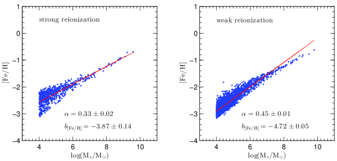
Figure 6.— The stellar metallicity – stellar mass correlations of the MW dwarfs obtained from models with different reionization strength. The left panel gives the result of the fiducial model; and the right panel shows the result for the model with all other parameters, except for the reionization strength, being the same as those in the fiducial model. The line and the points have the same meaning as those in Figure 4. As seen from the figure, reducing the reionization strength leads to an increase of the slope of the correlation. See details in Section 3.1.2.

Figure 7.— Comparison of the stellar mass – metallicity correlations obtained from the different reionization models. The blue dots are the results of the weak reionization model, and the green dots are obtained from the strong reionization model. As seen from the figure, the change of the reionization strength mainly affects the metallicity of the low-mass galaxies at $M_{*}\lesssim 4\times 10^{6}{\,M_{\odot}}$. See details in Section 3.1.2.

3.1.3 Effects of molecular hydrogen cooling

Figure 8 shows the correlations obtained from the models with and without including the ${\rm H}_{2}$ cooling in the early universe. As seen from the figure, these correlations are almost the same, insensitive to the molecular hydrogen cooling process. The reason is that molecular hydrogen cooling can only occur before the completion of the reionization when the UV background is not too strong, and it can be important only for small halos where the atomic cooling of gas is not effective; thus the stars formed through the cold gas cooled by molecular hydrogen cooling are only a very small part ($<5\%$) of the final stellar populations of a given satellite, which cannot affect the average stellar metallicity.

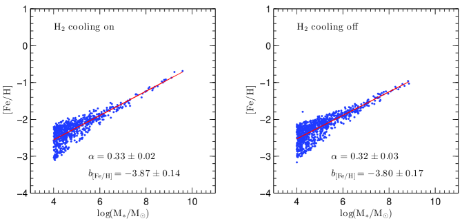
Figure 8.— The stellar mass – metallicity correlations obtained from models with including ${\rm H}_{2}$ cooling (on) and excluding it (off). All the other parameters are the same as those in the fiducial model. The line and the points have the same meaning as those in Figure 4. The figure shows that the ${\rm H}_{2}$ cooling occurred in the early universe has little effects in the correlation. See also Section 3.1.3.

For view clarity, a summary of all the best-fit lines for the stellar mass –metallicity correlations obtained from the models shown in Figures 4–8 is given in Figure 9.

Figure 9.— A summary of all the best-fit lines for the stellar mass – metallicity correlations obtained from the models shown in Figures 4–8. The model parameters are labeled in the panel. The best-fit lines of some model parameter sets [$(v_{\rm hot},\alpha_{\rm hot})=(400{\rm\,km\,s^{-1}},3.2)$, $(v_{\rm hot},\alpha_{\rm hot})=(200{\rm\,km\,s^{-1}},4.0)$, and the one with excluding H₂ cooling] are hard to distinguished from that of the fiducial model visually, and we use the result of the fiducial model (thick solid line) to represent all of them.

3.2. The metallicity distribution of individual satellites

Figure 10 shows the metallicity distributions of the satellites generated by the fiducial model. The simulated satellites are classified according to their luminosities. The simulation results are shown in blue curves, and the red histograms in all the panels and the green histograms in the bottom panels represent the observational results in Kirby et al. (2011a). The five panels represent different $V$-band magnitude bins. From left top to right bottom, the five bins are classified as Fornax-like ($-13.5<M_{V}\leq-12.5$), Leo I-like ($-12.5<M_{V}\leq-11.5$), Sculptor-like ($-11.5<M_{V}\leq-10.5$), Leo II and Sextans-like ($-10.0<M_{V}\leq-9.2$) and Ursa Minor and Draco-like ($-9.2<M_{V}\leq-8.5$), respectively. In general, our simulations reproduce the observations, except for the high-metallicity peak of Fornax and the double peaks of Sculptor. However, there are also some observations supporting that Fornax has a lower metallicity, e.g., the peak being at [Fe/H]$\sim-1.3$ in the photometric metallicity distribution of Stetson et al. (1998), which agrees with the simulation results better. Recent observation by Hendricks et al. (2014) also gives a lower average metallicity for Fornax (green histogram in the top ‘Fornax-like’ panel), but it is still higher than our simulation result. For Sculptor, currently it is the only satellite showing a double-peaked metallicity distribution, so it is possible that this distribution comes from a special formation history which is too rare to be realized in the about $10$ MW-like hosts. In addition, the observational metallicity distribution of Sculptor reported in de Boer et al. (2012) has only one peak (see also Helmi et al. 2006), as shown by the green diagram in the top ‘Scupltor-like’ panel, which leads to a better agreement with our simulation results; even if the observational double-peaked distribution is true, the simulation result still captures some basic observational chemical characteristics of Sculptor, as they are in the same metallicity range in Figure 10.

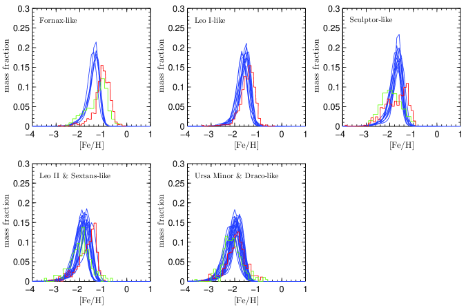
Figure 10.— The metallicity distributions of individual satellites. Different panels represent the satellites with different luminosity ranges. The blue curves represent our simulation results. The red histograms in all the panels and the green histograms in the bottom panels represent the observational distributions obtained from Kirby et al. (2011a); and the green histograms in the top ‘Fornax-like’ and ‘Sculptor-like’ panels represent the observational distributions obtained from Hendricks et al. (2014) and de Boer et al. (2012), respectively. The simulated distributions shown in the figure are obtained by convolving with a Gaussian function to model the observational errors, where the medians of the errors of the seven classical dSphs shown in Kirby et al. (2011a) is adopted, i.e., $0.12$ dex for Fornax-like, Leo I-like, and Sculptor-like satellites, $0.15$ dex for Leo II and Sextans-like satellites, and $0.18$ dex for Ursa Minor and Draco-like satellites. Our simulations roughly reproduce the observational results, except for the distributions in Fornax and Sculptor. See Section 3.2 for more discussion.

We introduce the following three quantities to characterize the metallicity distributions quantitatively.

• The first one is the corresponding [Fe/H] value at the peak of a metallicity distribution.

• The second one is based on the so-called linear metallicity dispersion, $\sigma({\cal Z})$, which is defined by (cf., Leaman 2010)

  $$\sigma({\cal Z})\equiv\left[\int({\cal Z}-\bar{{\cal Z}})^{2}P({\cal Z})d{\cal Z}\right]^{1/2},$$ (21)

  where ${\cal Z}\equiv 10^{\rm[Fe/H]}$, $P({\cal Z})$ is the metallicity distribution and $P({\cal Z})d{\cal Z}$ represents the mass fraction of the stars with metallicity in the range ${\cal Z}\rightarrow{\cal Z}+d{\cal Z}$, and

  $$\bar{{\cal Z}}\equiv\int{\cal Z}P({\cal Z})d{\cal Z}.$$ (22)

  The quantity of $\sigma({\cal Z})$ mainly evaluates the extension of the metal-rich tail of a metallicity distribution, because ${\cal Z}$ gives a relatively large weight to metal-rich stars for calculating $\sigma({\cal Z})$. As $\sigma({\cal Z})$ would be larger with larger $\bar{{\cal Z}}$, we employ the relative dispersion, $\sigma({\cal Z})/\bar{{\cal Z}}$, to represent the intrinsic extension of the metal-rich tails.

• The third one is also based on a dispersion, $\sigma({\cal Z}^{\prime})$, where ${\cal Z}^{\prime}\equiv\sqrt{1/10^{\rm[Fe/H]}}$, defined by the following equations similar to Equations (21) and (22):

  $$\sigma({\cal Z}^{\prime})\equiv\left[\int({\cal Z}^{\prime}-\bar{{\cal Z}^{\prime}})^{2}P({\cal Z}^{\prime})d{\cal Z}^{\prime}\right]^{1/2}$$ (23)

  and

  $$\bar{{\cal Z}^{\prime}}\equiv\int{\cal Z}^{\prime}P({\cal Z}^{\prime})d{\cal Z}^{\prime},$$ (24)

  where $P({\cal Z}^{\prime})$ is the distribution function of ${\cal Z}^{\prime}$ and $P({\cal Z}^{\prime})d{\cal Z}^{\prime}$ represents the mass fraction of the stars with ${\cal Z}^{\prime}$ in the range ${\cal Z}^{\prime}\rightarrow{\cal Z}^{\prime}+d{\cal Z}^{\prime}$. The quantity of ${\cal Z}^{\prime}$ gives a large weight to metal-poor stars and hence $\sigma({\cal Z}^{\prime})$ mainly represents the extension of the metal-poor tail of a metallicity distribution. Because $\sigma({\cal Z}^{\prime})$ would be larger with larger $\bar{{\cal Z}^{\prime}}$, we employ the relative dispersion, $\sigma({\cal Z}^{\prime})/\bar{{\cal Z}^{\prime}}$, to represent the intrinsic extension of the metal-poor tails. Note that for an appropriate representation of the metal-poor tails, we are careful in choosing the definition of ${\cal Z}^{\prime}$, for example, a square root is introduced into the definition to avoid the domination of the extremely metal-poor stars with [Fe/H]$<-5$ in the value of ${\cal Z}^{\prime}$, as the statistics of the extremely metal-poor stars is uncertain due to possible non-homogeneous mixing and turbulent dynamics of gas during their formation processes.

The corresponding [Fe/H] value at the peak of a metallicity distribution is roughly the same as the average [Fe/H] value, and the behavior of the average has been analyzed in Section 3.1, so in the following analysis we only focus on the two relative dispersions, $\sigma({\cal Z})/\bar{{\cal Z}}$ and $\sigma({\cal Z}^{\prime})/\bar{{\cal Z}^{\prime}}$, in Sections 3.2.1 and 3.2.2, respectively.

Figure 11 shows an example of $\sigma({\cal Z})/\bar{{\cal Z}}$ and $\sigma({\cal Z}^{\prime})/\bar{{\cal Z}^{\prime}}$ obtained from the fiducial model, in which both the original results from the simulations (small colored dots) and the statistical results (black solid circles and their error bars) are presented. As seen from the figure, the statistical results represent the general trends of the original results obtained from the simulations well. For simplicity and clarity, in the following similar figures indicating $\sigma({\cal Z})/\bar{{\cal Z}}$ and $\sigma({\cal Z}^{\prime})/\bar{{\cal Z}^{\prime}}$ (Figs. 12–15), we only show the statistical results of the solid circles and their error bars, but omit the original results of the small dots.

3.2.1 Metal-poor tails

We find that the metal-poor tails of the satellites in most of their stellar mass ranges are mainly constructed through minor mergers, except for some small satellites (with $M_{*}\sim 10^{3}$–$10^{5}{\,M_{\odot}}$). In general, the metallicity distribution of any galaxy has a metal-poor tail, and the stars in the metal-poor tail may come from star formation in the galaxy itself or from an accreted galaxy. We define a dispersion ratio of the metal-poor tails and show the logarithm of the ratio in the right panel of Figure 11 by color scales to indicate the relation of the metal-poor tail of a satellite with the stars accreted onto it in previous minor mergers occurred before the progenitor of the satellite falls into a big halo to become the satellite. Here the dispersion ratio of the metal-poor tails is defined by the ratio of $\sigma_{\rm remov}({\cal Z}^{\prime})/\sigma({\cal Z}^{\prime})$, where $\sigma({\cal Z}^{\prime})$ is derived from the stellar metallicity distribution of a present-day satellite, and $\sigma_{\rm remov}({\cal Z}^{\prime})$ is the dispersion of the metal-poor tail derived from the stellar metallicity distribution which is obtained by removing the stars accreted onto the satellite in previous minor mergers. As seen from the color distribution of the points in the right panel of the figure, the satellites at most of their stellar mass ranges have a low dispersion ratio, which indicates that minor mergers have a significant contribution to their metal poor tails; and only some small satellites (with $M_{*}\sim 10^{3}$–$10^{5}{\,M_{\odot}}$) have a high ratio, which indicates that the contribution from minor mergers is negligible. For those with relatively low dispersion ratios, in minor mergers, the accreted small galaxy usually has a lower metallicity, and the major part of its stellar population would appear in the metal-poor tail of the merged galaxy. In the minor mergers with relatively large mass ratios (e.g., not significantly lower than the mass ratio criterion $1/3$ for minor/major mergers), the mass of the stars in the accreted small galaxy is usually large than that of the metal-poor stars in the accreting large galaxy, and thus the stars in the accreted galaxy would dominate the properties of the metal-poor stars of the merged galaxy and hence the quantity of $\sigma({\cal Z}^{\prime})/\bar{{\cal Z}^{\prime}}$.

Some tendencies of $\sigma({\cal Z}^{\prime})/\bar{{\cal Z}^{\prime}}$ with different satellite masses are illustrated through the example of $\sigma({\cal Z}^{\prime})/\bar{{\cal Z}^{\prime}}$ shown in the right panel of Figure 11.

• The maximum $\sigma({\cal Z}^{\prime})/\bar{{\cal Z}^{\prime}}$ declines with increasing galaxy stellar mass. This can be understood as follows. Almost all the large $\sigma({\cal Z}^{\prime})/\bar{{\cal Z}^{\prime}}$, which form the upper boundary in Figure 11, are caused by minor mergers. The galaxies with low stellar masses usually formed earlier; and at the earlier time, minor mergers are more likely to have larger mass ratios, e.g. $1/5$, and thus the accreted galaxies have a larger contribution to the metal-poor tails of the merged galaxy.

• For relatively large satellites (e.g., with stellar mass above $10^{5.5}{\,M_{\odot}}$), the scatter in the values of $\sigma({\cal Z}^{\prime})/\bar{{\cal Z}^{\prime}}$ is small. For large satellites, their metal-poor tails are all constructed by minor mergers. Due to their relatively large stellar mass, it usually took a long time for them to form, and they would have accreted many small and metal-poor galaxies during their formation histories; and thus the properties of their metal-poor tails are determined by the sum of the metallicities of those accreted small galaxies. Although the metallicity of each individual accreted galaxies could be quite different, their sum has a relatively smaller scatter according to the central limit theorem. Furthermore, the average metallicities of these relatively large galaxies have a very small scatter as shown in the stellar metallicity versus stellar mass correlations above. Hence the scatter of the $\sigma({\cal Z}^{\prime})/\bar{{\cal Z}^{\prime}}$ of these relatively large galaxies is small.

• For relatively small satellites (e.g., with stellar mass below $10^{5.5}{\,M_{\odot}}$), the scatter in the values of $\sigma({\cal Z}^{\prime})/\bar{{\cal Z}^{\prime}}$ is large. For the small satellites, their formation durations are usually short, and not all of them have enough time to have experienced a minor merger. If a galaxy did not experience a minor merger, then the metal-poor tail is constructed by the stars formed in itself. Thus the extension of the metal-poor tail, or equivalently the value of the $\sigma({\cal Z}^{\prime})/\bar{{\cal Z}^{\prime}}$, is correlated to the star formation rate of this galaxy. With a higher star formation rate, the $\sigma({\cal Z}^{\prime})/\bar{{\cal Z}^{\prime}}$ would be lower, as less metal can involve into star formation and the stars tend to have the same metallicity. For these small galaxies, they can be formed with both large and small star formation rate, so the diversity of the $\sigma({\cal Z}^{\prime})/\bar{{\cal Z}^{\prime}}$ value is large.

The dependence of the $\sigma({\cal Z}^{\prime})/\bar{{\cal Z}^{\prime}}$ on the parameters of different physical processes is illustrated in the right panels of Figures 12–15. As seen from the figures, the statistical results of $\sigma({\cal Z}^{\prime})/\bar{{\cal Z}^{\prime}}$ are not sensitive to the used feedback parameters and the molecular hydrogen cooling process.

Figure 14 shows the statistical results of $\sigma({\cal Z}^{\prime})/\bar{{\cal Z}^{\prime}}$ for different reionization models. As seen from the right panel, $\sigma({\cal Z}^{\prime})/\bar{{\cal Z}^{\prime}}$ in the low-mass range $10^{3}\--10^{5}{\,M_{\odot}}$ is lower in the weak reionization model than that in the strong reionization model, but $\sigma({\cal Z}^{\prime})/\bar{{\cal Z}^{\prime}}$ in the mass range $10^{6}\--10^{8}{\,M_{\odot}}$ is higher in the weak reionization model than that in the strong reionization model. The reason for a lower $\sigma({\cal Z}^{\prime})/\bar{{\cal Z}^{\prime}}$ in the low-mass range $10^{3}\--10^{5}{\,M_{\odot}}$ resulting from the weak reionization model is that the host halos of those galaxies are smaller and thus experience fewer mergers than the corresponding ones in the strong reionization model. Furthermore, smaller halos lead to smaller disk specific angular momenta and higher star formation rates as mentioned in Section 3.1. Therefore, the metal-poor tail of a galaxy is weakened in the weak reionization model compared with that in the strong reionization model, no matter whether this tail is formed through minor mergers or star formation in itself. For galaxies in the mass range $10^{6}\--10^{8}{\,M_{\odot}}$, their metal-poor tails have significant contributions from the accreted smaller galaxies, as mentioned above. Although the enhancement of the SN feedback strength and the star formation rate in the small galaxies ($10^{3}\--10^{5}{\,M_{\odot}}$) reduces their stellar metallicities, the different reionization models cause limited effects on the average metallicities in larger galaxies ($10^{6}\--10^{8}{\,M_{\odot}}$), so the difference in the metallicities of the larger galaxies and the smaller accreted galaxies is enhanced by adopting weaker reionization, which prolongs the metal-poor tails of the larger galaxies.

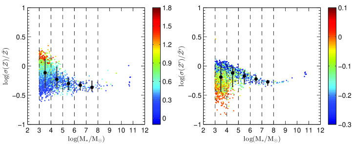
Figure 11.— An example for the relative metallicity dispersions $\sigma({\cal Z})/\bar{{\cal Z}}$ and $\sigma({\cal Z}^{\prime})/\bar{{\cal Z}^{\prime}}$ (see definitions in Eqs. 21–24) obtained from the fiducial model. The small colored dots show the original results from the simulations. The galaxies are further bound into five stellar mass bins, $10^{3}\--10^{4}{\,M_{\odot}}$, $10^{4}\--10^{5}{\,M_{\odot}}$, $10^{5}\--10^{6}{\,M_{\odot}}$, $10^{6}\--10^{7}{\,M_{\odot}}$, and $10^{7}\--10^{8}{\,M_{\odot}}$, indicated by the black dashed vertical lines. In each of these mass bins, the black solid circle represents the median of the small dots, and the error bar of each circle represents the range bounded by the lowest 10% and the highest 10% of the small dots. We do not show the statistical results for satellites with mass higher than $10^{8}{\,M_{\odot}}$ due to their small numbers. As seen from the figure, the statistical results can well present the major features of the original results. The color scale in the left panel represents $\Delta$[Fe/H]$\equiv$[Fe/H]${}_{\max}-\overline{\rm[Fe/H]}$, where [Fe/H]_max is the maximum value of the stellar [Fe/H] when the progenitor of a satellite falls into a big halo and $\overline{\rm[Fe/H]}$ is the average [Fe/H] at that time. The color scale in the right panel represents $\log[\sigma_{\rm remov}({\cal Z}^{\prime})/\sigma({\cal Z}^{\prime})]$, where $\sigma_{\rm remov}({\cal Z}^{\prime})$ is the dispersion of the metal-poor tail derived from the stellar metallicity distribution which is obtained by removing the stars accreted onto the satellite in previous minor mergers. The color distributions in the left panel indicates that the relative extension of the metal-rich tail of a satellite is usually formed before the progenitor of the satellite falls into a big halo to become the satellite, and the star formation after infall has negligible effects to the final shape of the metal-rich tail. The color distributions in the right panel indicates that the metal-poor tails of the satellites in most of their stellar mass ranges are mainly constructed through minor mergers, except for some small satellites (with $M_{*}\sim 10^{3}$–$10^{5}{\,M_{\odot}}$). See details in Section 3.2.

3.2.2 Metal-rich tails

We find that in the fiducial model, the relative extension of the metal-rich tail of a satellite is usually formed before the progenitor of the satellite falls into a big halo to become the satellite, and the star formation after infall has negligible effects to the final shape of the metal-rich tail. We define $\Delta$[Fe/H]$\equiv$[Fe/H]${}_{\max}-\overline{\rm[Fe/H]}$ and show it in the left panel of Figure 11 by color scales to indicate the relation of the metal-rich tails of the satellites with infall, where [Fe/H]_max is the maximum value of the stellar [Fe/H] when the progenitor of the satellite falls into a big halo and $\overline{\rm[Fe/H]}$ is the average [Fe/H] at that time (note that the definition of such a variable to illustrate this relation is not unique). As seen from the color distribution of the points in Figure 11, most of the satellites with low $\sigma({{\cal Z}})/\bar{{\cal Z}}$ have a low $\Delta$[Fe/H] and those with high $\sigma({{\cal Z}})/\bar{{\cal Z}}$ have a high $\Delta$[Fe/H]. Only some small satellites (with $M_{*}\sim 10^{3}$–$10^{5}{\,M_{\odot}}$) have a high $\Delta$[Fe/H]. For those with low $\Delta$[Fe/H] at infall, a strong-enough star formation and chemical enrichment after infall should be required to increase the extension of the metal-rich tails. However, after infall, the original halo of the galaxy may be tidally disrupted in the big halo, and the effect of SN feedback is very strong in the fiducial model. The strong feedback would strongly restrict the number of the stars that can be formed in the post-infall stage, which limits the possible value and the scatter range of $\sigma({\cal Z})/\bar{{\cal Z}}$. This is why the $\sigma({\cal Z})/\bar{{\cal Z}}$ values shown in Figure 11 appear flat over stellar masses and has small scatters for relatively large galaxies (with stellar mass $10^{5}\--10^{8}{\,M_{\odot}}$). The scatter in the galaxies with stellar mass above $10^{8}{\,M_{\odot}}$ begins to increase, as the feedback in these large galaxies is not as strong as that in those smaller galaxies.

The scatter of $\sigma({\cal Z})/\bar{{\cal Z}}$ becomes very large in the very small stellar mass range, i.e., $10^{3}\--10^{5}{\,M_{\odot}}$. The reason can be understood as follows. These small galaxies are formed in small halos and the amount of gas for star formation is small. It is possible that the majority of the gas in some galaxies (with high $\Delta$[Fe/H]) has turned into stars before infall, and thus the relatively large extension of their metal-rich tails are actually formed before infall, when SN feedback is much weaker than that after infall. The weak feedback strength leads to a strong metal-rich tail. For the galaxies whose metal-rich tails are not quite extended before infall, their $\sigma({\cal Z})/\bar{{\cal Z}}$ are similar to those of larger galaxies. For larger galaxies, their halos are larger and contains more gas, and generally they do not turn a large part of the gas into stars before infall, so their $\sigma({\cal Z})/\bar{{\cal Z}}$ are not large.

The dependence of the metal-rich tails on different physical processes are illustrated in the left panels of Figures 12-15.

• Figure 12 shows the statistical result of $\sigma({\cal Z})/\bar{{\cal Z}}$ obtained from the models with different $v_{\rm hot}$. The models with $v_{\rm hot}=400{\rm\,km\,s^{-1}}$ and $v_{\rm hot}=200{\rm\,km\,s^{-1}}$ have almost the same dispersions, because in these two cases the feedback strength provided by the scaling law is too strong to have significant star formation after infall. As $v_{\rm hot}$ decreases to $100{\rm\,km\,s^{-1}}$ or even $50{\rm\,km\,s^{-1}}$, the effects of different $v_{\rm hot}$ begin to appear, and the galaxies tend to have higher $\sigma({\cal Z})/\bar{{\cal Z}}$, because the weaker feedback allows more stars to be formed and more efficient metal enrichment.

• Figure 13 shows the statistical result of $\sigma({\cal Z})/\bar{{\cal Z}}$ obtained from the models with different $\alpha_{\rm hot}$. For $\alpha_{\rm hot}=4.0$ and $\alpha_{\rm hot}=3.2$, the dispersions are the same. This is again because the feedback in these two cases strongly suppresses the star formation in the post-infall stage. With $\alpha_{\rm hot}=2.0$, the feedback is weakened, which allows the formation of more metal-rich stars, enhances the metal-rich tails of the distributions, and thus increases $\sigma({\cal Z})/\bar{{\cal Z}}$. This figure also shows the results obtained from the model with $\alpha_{\rm hot}=3.2$ and $v_{\rm hot}=100{\rm\,km\,s^{-1}}$ for comparison, which are similar to those of the model with $\alpha_{\rm hot}=2.0$ and $v_{\rm hot}=200{\rm\,km\,s^{-1}}$. The degeneracy of the models with $\alpha_{\rm hot}=3.2$, $v_{\rm hot}=100{\rm\,km\,s^{-1}}$ and $\alpha_{\rm hot}=2.0$, $v_{\rm hot}=200{\rm\,km\,s^{-1}}$ can be understood from Figure 2, in which the lines representing the SN feedback efficiency of the two models (with circles and with triangles) are close.

• Figure 14 shows the statistical results of $\sigma({\cal Z})/\bar{{\cal Z}}$ obtained from different reionization models. As seen from the left panel, $\sigma({\cal Z})/\bar{{\cal Z}}$ obtained in the weak reionization model is higher than that in the strong reionization model. This can be understood as follows. As pointed out in Section 3.1, given the stellar mass of a galaxy, reducing reionization strength shifts its formation into lower mass halos, and increases its disk circular velocity and the galaxy star formation rate, which would enhance the possibility for a galaxy turning the majority of the gas into stars before its infall, and thus enhance the metal-rich tail. Furthermore, a larger disk circular velocity would also reduce the feedback coefficient $\beta$ and help to enhance the star formation after infall. For the very small galaxies ($10^{3}\--10^{4}{\,M_{\odot}}$), the enhancement is limited, because even with strong reionization, a part of them can still turn the majority of the gas into stars before infall. But for galaxies in $10^{4}\--10^{6}{\,M_{\odot}}$, the enhancement of metal-rich tails is quite obvious. This enhancement becomes small again in more massive mass range $10^{6}\--10^{8}{\,M_{\odot}}$, because reionization cannot strongly affect the more massive dark matter halos as mentioned before.

• Figure 15 shows the statistical results of $\sigma({\cal Z})/\bar{{\cal Z}}$ obtained from models with and without including molecular hydrogen cooling processes. These two models give almost the same dispersions, which means that the meal-rich tails are not sensitive to the molecular hydrogen cooling process. This is easily understood as follows. Molecular hydrogen cooling is only expected to work before the accomplishment of reionization, after which the UV background would strongly dissociate hydrogen molecules and suppress this cooling mechanism. It is only important for very small halos, and hence is unlikely to contribute to the metal-rich tails of satellites which are formed at lower redshift and in relatively large halos.

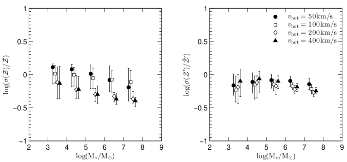
Figure 12.— Metallicity dispersions for different $v_{\rm hot}$. The parameters other than $v_{\rm hot}$ all have the same values as those for the fiducial model. The points and the error bars have the same meanings as those in Figure 11. For view clarity, the points in the same stellar mass bin are shifted horizontally a little one another. As seen from the figure, the metal-poor tails are not sensitive to $v_{\rm hot}$, while the metal-rich tails are sensitive to the reduction of the SN feedback strength through reducing $v_{\rm hot}$. For more details, see the caption of Figure 11 and Section 3.2.

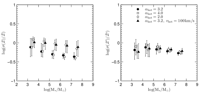
Figure 13.— Metallicity dispersions for different $\alpha_{\rm hot}$. All the other parameters not labeled in the figure have the same values as those for the fiducial model. The points and the error bars have the same meanings as those in Figure 11. As seen from the figure, the metal-poor tails are not sensitive to $\alpha_{\rm hot}$; while the metal-rich tails are sensitive to the reduction of the SN feedback strength through reducing $\alpha_{\rm hot}$ (note that some degeneracy exists in the results obtained from different $v_{\rm hot}$ and $\alpha_{\rm hot}$). For more details, see the caption of Figure 11 and Section 3.2.

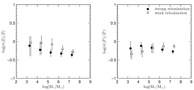
Figure 14.— Metallicity dispersions of different reionization models. All the other parameters are the same as those for the fiducial model. The points and the error bars have the same meanings as those in Figure 11. This figure indicates that different reionization strength can cause different effects on both metal-poor and metal-rich tails. For more details, see the caption of Figure 11 and Section 3.2.

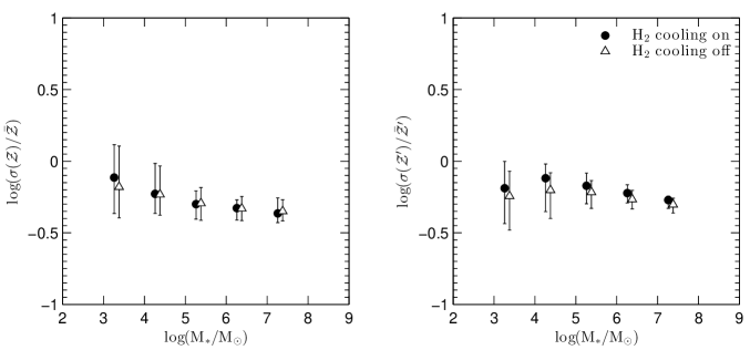
Figure 15.— Metallicity dispersions obtained with and without including ${\rm H}_{2}$ cooling. All the other parameters are the same as those for the fiducial model. The points and the error bars have the same meanings as those in Figure 11. The figure indicates that neither metal-poor tails nor metal-rich tails are sensitive to the ${\rm H}_{2}$ cooling process. For more details, see the caption of Figure 11 and Section 3.2.

4. Discussions

We have studied the behaviors of various metallicity properties under different physical conditions, and these metallicity properties can be used to put constraints on the underlying physical processes of galaxy formation, such as reionization and SN feedback.

4.1. Constraints on the reionization model

Kirby et al. (2013) measure the slopes of the stellar metallicity – luminosity correlation and the stellar metallicity – stellar mass correlation for the MW satellites and find $\alpha_{\rm obs}=0.29\pm 0.02$ and $0.30\pm 0.02$, respectively. Among all the models mentioned in Section 3, the fiducial model with strong reionization provides a similar slope (note that the best-fit intercept obtained from the fiducial model is also roughly consistent with the observational correlation provided in Kirby et al. 2013). According to the change tendency of the correlation slope under different physical conditions obtained above, below we argue that it is unlikely to produce such a slope under the weak reionization model even by varying the other parameters in the different physical processes involved.

• Under the weak reionization model, if all the other parameters are the same as those in the fiducial model, we find that the slope of the correlation predicted by the simulation is about $0.45$, which is substantially steeper than the observational slope.

• The relatively steep slope predicted by the weak reionization model cannot be reduced by adjusting the molecular hydrogen cooling process. As indicated in Figure 4, the ${\rm H}_{2}$ cooling has very limited effects on the average stellar metallicities of larger satellites because the major parts of their stars are formed in atomic cooling halos. For small satellites, it enables the star formation in smaller halos, and thus leads to an earlier enrichment. So turning off molecular hydrogen cooling can only delay the enrichment and thus reduce the average metallicities of small galaxies. And this would only increase the slope rather than reduce it.

• The relatively steep slope predicted by the weak reionization model cannot be reduced by increasing the SN feedback efficiency. As shown in Figure 2, the feedback strength predicted by the scaling law with the fiducial model parameters has already been very high to be limited by the energy condition, so there is no much difference in the results by further increasing the feedback strength.

• The relatively steep slope predicted by the weak reionization model cannot be reduced by decreasing the SN feedback efficiency, i.e., through decreasing $v_{\rm hot}$ or $\alpha_{\rm hot}$ in the scaling law (Eq. 3).

  • Reducing $v_{\rm hot}$ preferentially increases the slope of stellar metallicity – stellar mass correlation, which can be understood as follows. Reducing $v_{\rm hot}$ would cause a uniform suppression of the feedback efficiency expected by the scaling law. Galaxy formation processes can be affected if the expected feedback strength is lower than the limit set by the energy condition, which is relatively easier to occur for relatively large galaxies, e.g., $M_{*}\sim 10^{6}{\,M_{\odot}}$ or higher. So reducing $v_{\rm hot}$ would preferentially enhance the metallicities of relatively large galaxies, and thus increase the slope of stellar metallicity – stellar mass correlation, which is supported by Figure 4 (though the results are for the strong reionization model, for galaxies more massive than $10^{6}{\,M_{\odot}}$ the effects of the reionization are weak). Our simulation results show that reducing $v_{\rm hot}$ to $100{\rm\,km\,s^{-1}}$ increases the slope from $0.33$ to $0.4$, and further reducing $v_{\rm hot}$ to $50{\rm\,km\,s^{-1}}$ destroys the correlation.

  • Reducing $\alpha_{\rm hot}$ causes a suppression of the SN feedback efficiency preferentially in small galaxies. This may increase the metallicities of small galaxies while keep those of relatively large galaxies unchanged, so it may reduce the slope of the metallicity – stellar mass correlation. The lower boundary of $\alpha_{\rm hot}$ is $2.0$, which is set by the energy condition. We find that reducing $\alpha_{\rm hot}$ from 3.2 to 2.0 in the weak reionization model does reduce the slope, from $0.45$ to $0.43$; however, the reduced slope is still too large to be consistent with the observational one.

Hence the observed slope of the stellar mass – metallicity correlation strongly prefers the strong reionization model. As mentioned in Section 2, the weak reionization model is close to or slightly later than the cosmic average reionization epoch and the strong reionization model is probably earlier than the cosmic average. The strong reionization model implies that the region around the MW or the local group is reionized earlier than the cosmic average, or there is also a non-negligible contribution from the local ionizing radiation field in additional to the global ionizing background. This is in agreement with the conclusion drawn in Font et al. (2011). Our results support the patchy reionization scenario (Lunnan et al., 2012), in which the reionization is inhomogeneous and the reionization redshifts for different halos are different. Note that our work tests the patchy properties on relatively large scales (i.e., the host halo scale $\sim 300{\rm\,kpc}$), that is, the reionization is patchy at least on the scales comparable to the MW host halo or the local group size.

Apart from the slope, $\sigma({\cal Z}^{\prime})/\bar{{\cal Z}^{\prime}}$ is also mainly affected by different reionization models (see Fig. 14). Future observations on it will further examine the constraint on the reionization strength.

4.2. Constraints on the SN feedback models

After the strong reionization is adopted, the observational slope in the stellar metallicity versus stellar mass correlation can also further put constraints on $v_{\rm hot}$.

• Figure 4 indicates that only the model with feedback that is strong enough can provide a relatively small slope. With $\alpha_{\rm hot}=3.2$, the slope produced by the models with $v_{\rm hot}=100{\rm\,km\,s^{-1}}$ or $v_{\rm hot}=50{\rm\,km\,s^{-1}}$ is too large to be consistent with the observation. We find that even if a larger $\alpha_{\rm hot}$ is adopted, it is still difficult for the models with a smaller $v_{\rm hot}$ to generate a slope consistent with observations. For example, if $\alpha_{\rm hot}$ is increased to 4.0, the slope is reduced only a little to 0.38, which is still larger than the observational value. Therefore the observational $\alpha_{\rm obs}=0.30\pm 0.02$ prefers the case of $v_{\rm hot}>100{\rm\,km\,s^{-1}}$.

• The model with $v_{\rm hot}=400{\rm\,km\,s^{-1}}$ gives almost the same results as that adopting $v_{\rm hot}=200{\rm\,km\,s^{-1}}$, because the feedback strength is limited by the energy condition, so these two values cannot be distinguished in the dwarf satellites.

• Assuming strong reionization and $v_{\rm hot}=200{\rm\,km\,s^{-1}}$, Figure 5 shows that the correlations resulting from the model with $\alpha_{\rm hot}=3.2$ and that with $\alpha_{\rm hot}=2.0$ are almost the same. The reason is that the change of the feedback strength is not very strong.

The metal-rich tails are more sensitive to the change in the feedback strength and may put some further constraints on $(v_{\rm hot},\alpha_{\rm hot})$. Figure 16 shows $\sigma({\cal Z})/\bar{{\cal Z}}$ obtained from different SN feedback parameters, together with the observations of $14$ satellites around the Milky Way taken from Leaman (2010). The observation of LMC, with $\log[\sigma({\cal Z})/\bar{{\cal Z}}]=-0.33$, is not shown in this figure, because the stellar mass of LMC is above $10^{9}{\,M_{\odot}}$, which is out of the range of the figure. It is reasonable to omit LMC because here the discussion focuses on the dwarfs with stellar mass between $10^{3}{\,M_{\odot}}$ and $10^{8}{\,M_{\odot}}$. The observation of another satellite, Bootes I, is not shown in Figure 16, either. The stellar mass of Bootes I is $2.9\times 10^{4}{\,M_{\odot}}$ (McConnachie, 2012), and it has an extremely low $\sigma({\cal Z})/\bar{{\cal Z}}$, $\sim 10^{-3}$, according to Leaman (2010), which is much lower than the values of all the other observed satellites with similar stellar masses. This would indicate that Bootes I is very special and beyond the scope of the model in our work.

Figure 16 shows some degeneracies in $(v_{\rm hot},\alpha_{\rm hot})$: the results obtained from the models with $(400{\rm\,km\,s^{-1}},2.0)$ and $(200{\rm\,km\,s^{-1}},3.2)$ are close, which can be understood from Figure 2 where the feedback efficiencies of the two sets of parameters are close. As seen from Figure 16, however, the result of the model with $(200{\rm\,km\,s^{-1}},2.0)$ is distinguishable from the above two. The observations on $\sigma({\cal Z})/\bar{{\cal Z}}$ prefer the models with $(v_{\rm hot},\alpha_{\rm hot})=(400{\rm\,km\,s^{-1}},2.0)$ and $(200{\rm\,km\,s^{-1}},3.2)$ to the model with $(200{\rm\,km\,s^{-1}},2.0)$.

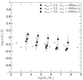
Figure 16.— Comparison of the observational metal-rich tails with the model results obtained with different SN feedback parameters. The open circles represent the observational results, where $\sigma({\cal Z})/\bar{{\cal Z}}$ are from Leaman (2010) and the stellar masses are from McConnachie (2012), for satellites SMC, Fornax, Sculptor, Sextans, Carina, Leo I, Leo II, CVn I, Seg I, Ursa Major I, Willman I, Draco, Ursa Minor and Hercules. The solid symbols and the error bars have the same meanings as those in Figure 11, and the parameters not labeled in the figure have the same settings as those in fiducial model. The figure indicates that the fiducial model (solid triangles) are generally consistent with the observational metal-rich tails well.

5. Summary

We have investigated the effects of the SN feedback, the reionization of the universe, and the molecular hydrogen cooling processes on the chemical properties of the dwarfs around the Milky Way-like host galaxies, through a semi-analytical galaxy formation model. Our fiducial model can reproduce the luminosity function, the stellar metallicity versus stellar mass correlation, and the distribution of the metal-rich tails of the MW dwarf satellites.

We find that the slope of the stellar metallicity versus stellar mass correlation is sensitive to the SN feedback parameter $v_{\rm hot}$, which can lead to a universal change of feedback strength among the whole satellite mass range. This slope is larger with smaller $v_{\rm hot}$, but a too small $v_{\rm hot}$ destroys the correlation. This slope is fairly not changing with $v_{\rm hot}$ when $v_{\rm hot}$ is above $200{\rm\,km\,s^{-1}}$, because the feedback strength expected by the feedback scaling law is too large so as to be limited by the energy condition.

We find that the slope of the stellar metallicity versus stellar mass correlation is also sensitive to the strength of the reionization process. The slope is flatter if the universe or the local universe is reionized earlier (i.e., reionization is stronger). The reason is that the halo of a given mass dwarf before infall is relatively more massive in a (local) universe with stronger reionization, which thus allows a more efficient metal enrichment.

Both the SN feedback and the reionization affect the slope, but in different satellite mass range. Feedback preferentially affects large dwarfs, because the feedback strength in small dwarfs is limited by the energy condition. The SN feedback affects the slope through affecting the metallicities of those large dwarfs, with mass above several $10^{6}{\,M_{\odot}}$. Reionization only strongly affects small halos, and thus it can only affect small dwarfs significantly. The reionization affects the slope through affecting the metallicities of the small dwarfs, with mass below $4\times 10^{6}{\,M_{\odot}}$.

We find that the metal-poor tail (quantified by $\sigma({\cal Z}^{\prime})/\bar{{\cal Z}^{\prime}}$) is sensitive to the reionization. With weaker reionization, the $\sigma({\cal Z}^{\prime})/\bar{{\cal Z}^{\prime}}$ of the satellites less massive than $10^{5}{\,M_{\odot}}$ are smaller, because weaker reionization increases the star formation rate and reduces the minor merger possibilities of the small galaxies, which leads to weaker metal poor tails; but the $\sigma({\cal Z}^{\prime})/\bar{{\cal Z}^{\prime}}$ of more massive satellites are larger, because weaker reionization lowers stellar metallicities in these small galaxies, while the metal-poor tails of larger galaxies are contributed mainly by the small galaxies through mergers, and the reduction of the stellar metallicities of the small galaxies enhances the metal-poor tails of the larger galaxies.

We find that the strength of the metal-rich tail (quantified by $\sigma({\cal Z})/\bar{{\cal Z}}$) is sensitive to feedback parameters. With weaker feedback, the tails are stronger. This is because weaker feedback allows more efficient metal enrichment and more metal-rich stars to form and thus enhances the metal-rich tails.

We find that both the metallicity - stellar mass correlation and the metallicity distribution in individual satellites are not sensitive to molecular hydrogen cooling, as it only affects the formation of a very small part of stars in dwarfs.

The various chemical properties can be used to constrain the underlying physical processes of galaxy formation. The observed slope ($0.30\pm 0.02$) of the stellar metallicity – stellar mass correlation prefers the strong reionization, which suggests that the universe is reionized at a redshift $\gtrsim 10$ or the local universe is reionized earlier than the cosmic average due to the contribution from the local reionizing sources. This slope also prefers $v_{\rm hot}>100{\rm\,km\,s^{-1}}$. The observations on $\sigma({\cal Z})/\bar{{\cal Z}}$ can put constraints on $\alpha_{\rm hot}$: they prefer the models with $(v_{\rm hot},\alpha_{\rm hot})=(400{\rm\,km\,s^{-1}},2.0)$ and $(200{\rm\,km\,s^{-1}},3.2)$ over the model with $(200{\rm\,km\,s^{-1}},2.0)$. There are some degeneracies between $v_{\rm hot}$ and $\alpha_{\rm hot}$, for example, the results of $(v_{\rm hot},\alpha_{\rm hot})=(400{\rm\,km\,s^{-1}},2.0)$ and $(200{\rm\,km\,s^{-1}},3.2)$ are close.

Appendix: Gas cooling recipe

The gas cooling rate in a DM halo at time $t$, $\dot{M}_{\rm cool}(t)$, is calculated by

$$\dot{M}_{\rm cool}(t)=\frac{M_{\rm gas}[r_{\rm min}(t+\Delta t)]-M_{\rm gas}[r_{\rm min}(t)]}{\Delta t},$$ (25)

where $M_{\rm gas}(r)$ is the total hot gas mass within radius $r$ of the DM halo and $r_{\rm min}(t)\equiv\min[r_{\rm cool}(t),r_{\rm ff}(t)]$. The $r_{\rm cool}(t)$ is the cooling radius and obtained by the following energy-conservation equation in the model of Cole et al. (2000):

$$\mu m_{\rm H}\rho_{\rm gas}(r_{\rm cool})\Lambda(T_{\rm gas},Z_{\rm gas})\cdot(t-t_{0})=\frac{3}{2}kT_{\rm gas},$$ (26)

where $\mu m_{\rm H}$ is the mean molecular mass of the hot gas, $k$ is the Boltzmann constant, $\rho_{\rm gas}(r)$ is the mass density of the hot gas at radius $r$, $\Lambda(T_{\rm gas},Z_{\rm gas})$ is the cooling function as a function of the gas temperature $T_{\rm gas}$ and metallicity $Z_{\rm gas}$ (Sutherland & Dopita, 1993), and $t_{0}$ is the beginning moment of the cooling. The $r_{\rm ff}$ is the free-fall radius obtained from the solution of $t_{\rm ff}(r)=t-t_{0}$, where $t_{0}$ is the beginning moment of the cooling process, $t_{\rm ff}(r)$ is the free-fall time taken by the materials to free fall to the center of the DM halo from radius $r$.

In the model of Cole et al. (2000), at the moment $t_{0}$, the mass density of the hot gas in a dark matter halo is assumed to follow a distribution with $\rho_{\rm gas}\propto 1/(r^{2}+r^{2}_{\rm core})$, where $r_{\rm core}$ is a parameter. The $T_{\rm gas}$ is set to be the virial temperature of the DM halo. The gas heated by the SN feedback (reheated gas) is assumed not to join the cooling process until the DM halo mass grows up to twice of the mass obtained at $t_{0}$. Once the DM halo mass doubles, the hot gas distribution is re-distributed to incorporate the previously reheated gas, and then the previously reheated gas joins the cooling process. This treatment partly realizes the processes in which as the dark matter halo grows, the gravitational potential changes and the hydrodynamical state of the hot gas also changes correspondingly. However, the reheated gas could cool down before the obvious change of the gravitational potential, which is roughly considered in the model of Bower et al. (2006). In that model, the reheated gas is assumed to join the cooling processes in a time scale comparable to the halo dynamical time scale. In this work, we calculate the cooling of this reheated gas by the following simple and more detailed treatments.

As the reheated gas is generated at a relatively late time, it is hotter than the original gas which begins to cool at $t_{0}$, and thus the reheated gas alone usually would not contribute much to the cooling rate $\dot{M}_{\rm cool}$. But if the reheated gas is mixed with the cooling hot gas since $t_{0}$, it can join an efficient cooling immediately. To calculate the degree of this mixing process, we assume that the mass density of the reheated gas follows the same profile shape as the original hot gas. As this mixing occurs before the significant change of the halo gravitational potential (i.e., the halo mass doubles), the parameter $r_{\rm core}$ is assumed not to be changed, while only the normalization of the distributions are different. The temperature of the reheated gas is set to the virial temperature of the DM halo. Because of the limited amount of the reheated gas, usually it can only distribute to an outermost radius $r_{\rm out}$ which is smaller than the DM halo’s virial radius $r_{\rm vir}$. If since time $t^{\prime}(>t_{0})$, $r_{\rm out}$ starts to be larger than $r_{\rm min}(t^{\prime})$, the reheated gas between $r_{\rm min}$ and $r_{\rm out}$ is mixed with the original hot gas which cools since $t_{0}$. The mixing is assumed to be homogeneous and changes the mass density of the hot gas between $r_{\rm min}$ and $r_{\rm out}$. We denote the total gas mass density after the mixing by $\rho^{\prime}_{\rm gas}$ and the metallicity by $Z^{\prime}_{\rm gas}$. After the mixing, we calculate the cooling radius $r_{\rm cool}$ from the solution of the following energy-conservation equation:

$$\mu m_{\rm H}\rho_{\rm gas}^{2}(r)\Lambda(T_{\rm gas},Z_{\rm gas})\cdot(t^{\prime}-t_{0})+\mu m_{\rm H}{\rho^{\prime}}^{2}_{\rm gas}(r)\times$$

$$\Lambda(T^{\prime}_{\rm gas},Z^{\prime}_{\rm gas})\cdot(t-t^{\prime})=\frac{3}{2}kT_{\rm gas}\rho^{\prime}_{\rm gas}(r),$$

and the free-fall radius $r_{\rm ff}$ from the solution of the following equation:

$$\rho^{\prime}_{\rm gas}(r)=\rho_{\rm gas}(r)\cdot(t^{\prime}-t_{0})/t_{\rm ff}(r)+\rho^{\prime}_{\rm gas}\cdot(t-t^{\prime})/t_{\rm ff}(r).$$ (28)

References

- Abel et al. (2002) Abel, T., Bryan, G. L., & Norman, M. L. 2002, Science, 295, 93
- Becker et al. (2001) Becker, R. H., Fan, X., White, R. L., et al. 2001, AJ, 122, 2850
- Benson (2010) Benson, A. J. 2010, Physics Reports, 495, 33
- Benson & Bower (2010) Benson, A. J., & Bower, R. 2010, MNRAS, 405, 1573
- Benson et al. (2003) Benson, A. J., Bower, R. G., Frenk, C. S., et al. 2003, ApJ, 599, 38
- Benson et al. (2002) Benson, A. J., Frenk, C. S., Lacey, C. G., Baugh, C. M., & Cole, S. 2002, MNRAS, 333, 177
- Benson et al. (2006) Benson, A. J., Sugiyama, N., Nusser, A., & Lacey, C. G. 2006, MNRAS, 369, 1055
- Bett et al. (2007) Bett, P., Eke, V., Frenk, C. S., et al. 2007, MNRAS, 376, 215
- de Blok (2010) de Blok, W. J. G. 2010, Advances in Astronomy, 2010, 789293
- de Boer et al. (2012) de Boer, T. J. L., Tolstoy, E., Hill, V., et al. 2012, A&A, 539, A103
- Bovill & Ricotti (2009) Bovill, M. S., & Ricotti, M. 2009, ApJ, 693, 1859
- Bower et al. (2006) Bower, R. G., Benson, A. J., Malbon, R., et al. 2006, MNRAS, 370, 645
- Bower et al. (2010) Bower, R. G., Vernon, I., Goldstein, M., et al. 2010, MNRAS, 407, 2017
- Boylan-Kolchin et al. (2013) Boylan-Kolchin, M., Bullock, J. S., Sohn, S. T., Besla, G., van der Marel, R. P. 2013, ApJ, 767, 140
- Bromm (2013) Bromm, V. 2013, Reports on Progress in Physics, 76, 112901
- Bromm et al. (2002) Bromm, V., Coppi, P. S., & Larson, R. B. 2002, ApJ, 564, 23
- Brooks et al. (2013) Brooks, A. M., Kuhlen, M., Zolotov, A., & Hooper, D. 2013, ApJ, 765, 22
- Bullock et al. (2000) Bullock, J. S., Kravtsov, A. V., & Weinberg, D. H. 2000, ApJ, 539, 517
- Busha et al. (2010) Busha, M. T., Alvarez, M. A., Wechsler, R. H., Abel, T., & Strigari, L. E. 2010, ApJ, 710, 408
- Carigi et al. (2002) Carigi, L., Hernandez, X., & Gilmore, G. 2002, MNRAS, 334, 117
- Chabrier (2003) Chabrier, G. 2003, PASP, 115, 763
- Cole et al. (2000) Cole, S., Lacey, C. G., Baugh, C. M., & Frenk, C. S. 2000, MNRAS, 319, 168
- Cole & Lacey (1996) Cole, S., & Lacey, C. 1996, MNRAS, 281, 716
- Croton et al. (2006) Croton, D. J., Springel, V., White, S. D. M., et al. 2006, MNRAS, 365, 11
- Diemand et al. (2007) Diemand, J., Kuhlen, M., & Madau, P. 2007, ApJ, 657, 262
- Fenner et al. (2006) Fenner, Y., Gibson, B. K., Gallino, R., & Lugaro, M. 2006, ApJ, 646, 184
- Font et al. (2011) Font, A. S., Benson, A. J., Bower, R. G., et al. 2011, MNRAS, 417, 1260
- Frebel et al. (2010) Frebel, A., Kirby, E. N., & Simon, J. D. 2010, Nature, 464, 72
- Galli & Palla (1998) Galli, D., & Palla, F. 1998, A&A, 335, 403
- Geha et al. (2009) Geha, M., Willman, B., Simon, J. D., et al. 2009, ApJ, 692, 1464
- Gnedin (2000) Gnedin, N. Y. 2000, ApJ, 542, 535
- Grebel & Gallagher (2004) Grebel, E. K., & Gallagher, J. S., III 2004, ApJ, 610, L89
- Guo et al. (2011) Guo, Q., White, S., Boylan-Kolchin, M., et al. 2011, MNRAS, 413, 101
- Helmi et al. (2006) Helmi, A., Irwin, M. J., Tolstoy, E., et al. 2006, ApJ, 651, L121
- Hendricks et al. (2014) Hendricks, B., Koch, A., Lanfranchi, G. A., et al. 2014, ApJ, 785, 102
- Hinshaw et al. (2013) Hinshaw, G., Larson, D., Komatsu, E., et al. 2013, ApJS, 208, 19
- Iwamoto et al. (1999) Iwamoto, K., Brachwitz, F., Nomoto, K., et al. 1999, ApJS, 125, 439
- Kauffmann et al. (1993) Kauffmann, G., White, S. D. M., & Guiderdoni, B. 1993, MNRAS, 264, 201
- Kirby et al. (2011a) Kirby, E. N., Lanfranchi, G. A., Simon, J. D., Cohen, J. G., & Guhathakurta, P. 2011a, ApJ, 727, 78
- Kirby et al. (2011b) Kirby, E. N., Cohen, J. G., Smith, G. H., et al. 2011b, ApJ, 727, 79
- Kirby et al. (2013) Kirby, E. N., Cohen, J. G., Guhathakurta, P., et al. 2013, ApJ, 779, 102
- Klypin et al. (1999) Klypin, A., Kravtsov, A. V., Valenzuela, O., & Prada, F. 1999, ApJ, 522, 82
- Koposov et al. (2008) Koposov, S., Belokurov, V., Evans, N. W., et al. 2008, ApJ, 686, 279
- Koposov et al. (2009) Koposov, S. E., Yoo, J., Rix, H.-W., et al. 2009, ApJ, 696, 2179
- Kravtsov et al. (2004) Kravtsov, A. V., Gnedin, O. Y., & Klypin, A. A. 2004, ApJ, 609, 482
- Lanfranchi & Matteucci (2003) Lanfranchi, G. A., & Matteucci, F. 2003, MNRAS, 345, 71
- Lanfranchi & Matteucci (2004) Lanfranchi, G. A., & Matteucci, F. 2004, MNRAS, 351, 1338
- Leaman (2010) Leaman, R. 2012, AJ, 144, 183
- Lemson & Kauffmann (1999) Lemson, G., & Kauffmann, G. 1999, MNRAS, 302, 111
- Li et al. (2010) Li, Y.-S., de Lucia, G., & Helmi, A. 2010, MNRAS, 401, 2036
- Lu et al. (2012) Lu, Y., Mo, H. J., Katz, N., & Weinberg, M. D. 2012, MNRAS, 421, 1779
- Lu et al. (2011) Lu, Y., Mo, H. J., Weinberg, M. D., & Katz, N. 2011, MNRAS, 416, 1949
- Lunnan et al. (2012) Lunnan, R., Vogelsberger, M., Frebel, A., Hernquist, L., Lidz, A., & Boylan-Kolchin, M. 2012, ApJ, 746, 109
- Macciò et al. (2010) Macciò, A. V., Kang, X., Fontanot, F., et al. 2010, MNRAS, 402, 1995
- Maoz et al. (2010) Maoz, D., Sharon, K., & Gal-Yam, A. 2010, ApJ, 722, 1879
- Marcolini et al. (2006) Marcolini, A., D’Ercole, A., Brighenti, F., & Recchi, S. 2006, MNRAS, 371, 643
- Marcolini et al. (2008) Marcolini, A., D’Ercole, A., Battaglia, G., & Gibson, B. K. 2008, MNRAS, 386, 2173
- Martin et al. (2008) Martin, N. F., de Jong, J. T. A., & Rix, H.-W. 2008, ApJ, 684, 1075
- Martin et al. (2007) Martin, N. F., Ibata, R. A., Chapman, S. C., Irwin, M., & Lewis, G. F. 2007, MNRAS, 380, 281
- Matteucci & Recchi (2001) Matteucci, F., & Recchi, S. 2001, ApJ, 558, 351
- McConnachie (2012) McConnachie, A. W. 2012, AJ, 144, 4
- Moore et al. (1999) Moore, B., Ghigna, S., Governato, F., et al. 1999, ApJ, 524, L19
- Mortlock et al. (2011) Mortlock, D. J., Warren, S. J., Venemans, B. P., et al. 2011, Nature, 474, 616
- Muñoz et al. (2009) Muñoz, J. A., Madau, P., Loeb, A., & Diemand, J. 2009, MNRAS, 400, 1593
- Nagashima et al. (2005a) Nagashima, M., Lacey, C. G., Baugh, C. M., Frenk, C. S., & Cole, S. 2005, MNRAS, 358, 1247
- Nagashima et al. (2005b) Nagashima, M., Lacey, C. G., Okamoto, T., et al. 2005, MNRAS, 363, L31
- Nomoto et al. (2006) Nomoto, K., Tominaga, N., Umeda, H., Kobayashi, C., & Maeda, K. 2006, Nuclear Physics A, 777, 424
- Okamoto et al. (2008) Okamoto, T., Gao, L., & Theuns, T. 2008, MNRAS, 390, 920
- Parkinson et al. (2008) Parkinson, H., Cole, S., & Helly, J. 2008, MNRAS, 383, 557
- Planck Collaboration et al. (2013) Planck Collaboration, Ade, P. A. R., Aghanim, N., et al. 2013, arXiv:1303.5076
- Robertson et al. (2005) Robertson, B., Bullock, J. S., Font, A. S., Johnston, K. V., & Hernquist, L. 2005, ApJ, 632, 872
- Rocha et al. (2012) Rocha, M., Peter, A. H. G., & Bullock, J. 2012, MNRAS, 425, 231
- Romano & Starkenburg (2013) Romano, D., & Starkenburg, E. 2013, MNRAS, 434, 471
- Salvadori & Ferrara (2009) Salvadori, S., & Ferrara, A. 2009, MNRAS, 395, L6
- Simon & Geha (2007) Simon, J. D., & Geha, M. 2007, ApJ, 670, 313
- Simon et al. (2011) Simon, J. D., Geha, M., Minor, Q. E., et al. 2011, ApJ, 733, 46
- Somerville (2002) Somerville, R. S. 2002, ApJ, 572, L23
- Somerville & Kolatt (1999) Somerville, R. S., & Kolatt, T. S. 1999, MNRAS, 305, 1
- Somerville & Primack (1999) Somerville, R. S., & Primack, J. R. 1999, MNRAS, 310, 1087
- Springel et al. (2008) Springel, V., Wang, J., Vogelsberger, M., et al. 2008, MNRAS, 391, 1685
- Starkenburg et al. (2013) Starkenburg, E., Helmi, A., De Lucia, G., et al. 2013, MNRAS, 429, 725
- Stetson et al. (1998) Stetson, P. B., Hesser, J. E., & Smecker-Hane, T. A. 1998, PASP, 110, 533
- Strigari et al. (2007) Strigari, L. E., Bullock, J. S., Kaplinghat, M., et al. 2007, ApJ, 669, 676
- Strigari et al. (2008) Strigari, L. E., Bullock, J. S., Kaplinghat, M., et al. 2008, Nature, 454, 1096
- Sutherland & Dopita (1993) Sutherland, R. S., & Dopita, M. A. 1993, ApJS, 88, 253
- Tollerud et al. (2008) Tollerud, E. J., Bullock, J. S., Strigari, L. E., & Willman, B. 2008, ApJ, 688, 277
- van den Bergh (2000) van den Bergh S., 2000, The Galaxies of the Local Group, Cambridge Astrophys. Ser. Vol. 35. Cambridge Univ. Press, Cambridge
- Vargas et al. (2013) Vargas, L. C., Geha, M., Kirby, E. N., & Simon, J. D. 2013, ApJ, 767, 134
- White & Frenk (1991) White, S. D. M., & Frenk, C. S. 1991, ApJ, 379, 52
- Wyithe & Loeb (2006) Wyithe, J. S. B., & Loeb, A. 2006, Nature, 441, 322
- Wyithe & Loeb (2013) Wyithe, J. S. B., & Loeb, A. 2013, MNRAS, 428, 2741
- Yates et al. (2013) Yates, R. M., Henriques, B., Thomas, P. A., et al. 2013, MNRAS, 435, 3500
- Zucker et al. (2006) Zucker, D. B., Belokurov, V., Evans, N. W., et al. 2006, ApJ, 643, L103