The masses of young stars:
CN as a probe of dynamical masses.

Abstract

Aims. We attempt to determine the masses of single or multiple young T Tauri and HAeBe stars from the rotation of their Keplerian disks.

Methods. We used the IRAM PdBI interferometer to perform arcsecond resolution images of the CN N=2-1 transition with good spectral resolution. Integrated spectra from the 30-m radiotelescope show that CN is relatively unaffected by contamination from the molecular clouds. Our sample includes 12 sources, among which isolated stars like DM Tau and MWC 480 are used to demonstrate the method and its accuracy. We derive the dynamical mass by fitting a disk model to the emission, a process giving M/D the mass to distance ratio. We also compare the CN results with higher resolution CO data, that are however affected by contamination.

Results. All disks are found in nearly perfect Keplerian rotation. We determine accurate masses for 11 stars, in the mass range 0.5 to 1.9$M_{\odot}$. The remaining one, DG Tau B, is a deeply embedded object for which CN emission partially arises from the outflow. With previous determination, this leads to 14 (single) stars with dynamical masses. Comparison with evolutionary tracks, in a distance independent modified HR diagram, show good overall agreement (with one exception, CW Tau), and indicate that measurement of effective temperatures are the limiting factor. The lack of low mass stars in the sample does not allow to distinguish between alternate tracks.

1 Introduction

To understand the diversity among the many known planetary systems it is important to study the evolution of their proto-planetary disks and to establish a reliable clock for the very early ($<10$ Myr) phases. Ages of the young stars that host the disks can provide the clocks. Unfortunately, the age of individual stars is not directly observable, and must rely on the comparison between the observed stellar properties and theoretical models of early stellar evolution, a model dependent derivation. From an observational point of view, stars can be characterized by their mass $M_{*}$, radius $R_{*}$, luminosity $L_{*}$ (or the equivalent combinations including effective temperature $T_{\mathrm{eff}}$ and surface gravity $g$), and detailed spectrum. Ages of young stars are usually derived through their location in, for example, an HR ($L_{*}\mathrm{\leavevmode\nobreak\ vs\leavevmode\nobreak\ }T_{\mathrm{eff}}$) diagram.

The existing stellar evolution models (Baraffe et al. 1998; D’Antona & Mazzitelli 1994, 1997; Palla & Stahler 1999; Siess et al. 2000), the Y2 models from Demarque et al. (2004, 2008), the Dartmouth models (Dotter et al. 2008), and the Pisa tracks (Tognelli et al. 2011), implement various approximations of the complex physics at work to compute stellar characteristics ($R_{*},L_{*},g,T_{\mathrm{eff}}$) as a function of input parameters. The main stellar parameters are mass $M_{*}$ and age, and the initial elemental composition (metallicity). After the initial models, the development of early stellar evolution models somewhat stagnated, largely because the models were not challenged by sufficiently accurate observations. Recent unexpected discoveries, such as that of the “twin” binary star Par 1802 (Stassun et al. 2008), have raised new questions and fostered new developments. Additional complexity such as stellar rotation (e.g. Maeder & Meynet 2005), magnetic fields (e.g. Macdonald & Mullan 2010; Morales et al. 2010), and the history of accretion (Baraffe & Chabrier 2010), starts being incorporated in existing models.

These models must be validated by comparison between their predictions and actual observations. Several possibilities exist: 1/ Radius $R_{*}$ is a primary characteristic, but its direct determination is only possible through optical/IR interferometric measurements within $\sim 25$ pc, or in the specific case of eclipsing binaries, and hence not suitable for distant young stars. 2/ Surface gravity $g$ can be derived from observed spectra, providing a proxy for the mass (through the $M_{*}\propto L_{*}gT_{\mathrm{eff}}^{-4}$ relation), but the mass uncertainty then scales as $D^{2}$. 3/ Metal depletion, essentially that of Li for young stars (e.g. White & Hillenbrand 2005), and pulsation modes from astero-seismologic measurements can also be age indicators, but are restricted to (very) limited ranges of age and mass for young stars. The only prime parameter that can be unambiguously compared with observations remains the stellar mass.

The Keplerian rotation of disks (Guilloteau & Dutrey 1998) is the only method that can be used to measure $M_{*}$, or more precisely $M_{*}/D$, the Mass to Distance ratio for single stars. As $L_{*}$ scales as $D^{2}$, stars can be accurately placed in a modified HR diagram: $L/M^{2}\mathrm{\leavevmode\nobreak\ vs\leavevmode\nobreak\ }T_{\mathrm{eff}}$, thereby canceling the impact of the distance uncertainty (that can be large for the star formation regions). Our pioneering work using this simple method indeed suggested that some of the available evolutionary models did not agree with these direct mass determinations (Simon et al. 2000). It was based on only 8 stars, but little progress has been made since. For isolated sources, CQ Tau was measured by Chapillon et al. (2008), and MWC 758 by Isella et al. (2010) using CO (but both stars suffer from large distance uncertainty, see Chapillon et al. 2008), while the mass of HH 30 (unfortunately a binary) was derived by Pety et al. (2006) from ¹³CO. For embedded sources, CO disk detections were reported by Schaefer et al. (2009) for LkHa 358, GO Tau, Haro 6-13 and Haro 6-33, and by Guilloteau et al. (2011) for FT Tau, but no accurate masses could be derived because of contamination of the disk emission by emission or absorption from their surrounding environments (clouds, envelopes and/or outflows) or from molecular clouds along the line of sight. The effectiveness of dynamical mass measurements is attested by the work of Rosenfeld et al. (2012), who compared the dynamical mass derived from CO observations of the circumbinary disk of VX 4046 Sgr to the mass obtained from the analysis of the radial velocity curves of this spectroscopic binary.

Piétu et al. (2007) and Dutrey et al. (2008) improved the results on DM Tau, LkCa 15, MWC 480, and GM Aur using CO isotopologues, and these 4 stars remain the only single young low mass stars with accurate masses.

Beating the contamination problem is a pre-requisite to determine accurate dynamical masses. In Guilloteau et al. (2013), we showed through a survey of 40 stars that CN N=2-1 transition is a good tracer for this purpose. It appears in general free of contamination from clouds, and is strong enough in many disks to be a sensitive tracer of the disk kinematics. We use here this property to study a sample of 12 stars in CN N=2-1 using high angular and spectral resolution spectro-imaging with the IRAM Plateau de Bure interferometer, and derive accurate masses for 11 of them.

2 Observations and Analysis

2.1 Source Sample

Our sample is derived from the study of Guilloteau et al. (2013). It includes all “bona-fide” disks with strong enough CN emission to be imaged in a short (4 hours per source) time with the IRAM interferometer. Sources exhibiting potential contamination from outflows or envelopes were deliberately excluded at this stage, with the exception of the enigmatic embedded object DG Tau B.

Our sample contains 12 stars: 9 T Tauri stars, one HAe (MWC 480) and two embedded objects, IRAS04302+2247 (the Butterfly star) and DG Tau B. All stars are single, except HV Tau, which is a triple system.

Data for the well known, isolated (from any surrounding cloud), objects like DM Tau, LkCa 15 and MWC 480 are taken from Chapillon et al. (2012). These sources have been observed in many other molecular lines, and thus serve as a probe of the reliability of CN as a dynamical mass tracer.

Newly observed sources include objects for which previous attempts to derive dynamical masses were affected by low S/N and contamination from molecular clouds: CY Tau, DL Tau by (Simon et al. 2000), and GO Tau by Schaefer et al. (2009). The remaining sources had no previous dynamical mass measurements: DN Tau and IQ Tau (which had been observed in ¹²CO by Schaefer et al. (2009) but not detected, presumably because of contamination by a molecular cloud), HV Tau, IRAS04302+2247 and DG Tau B.

2.2 Observations

All observations were carried out with the IRAM interferometer. DM Tau, LkCa 15 and MWC 480 have been reported by Chapillon et al. (2012). The characteristic angular resolution is $1.6\times 1.0^{\prime\prime}$ for DM Tau, and $1.3\times 0.8^{\prime\prime}$ for MWC 480 and LkCa 15 ($1.0\times 0.65^{\prime\prime}$ with uniform weighting) which have baselines as long as 330 m (250 k$\lambda$).

CI Tau, CY Tau and GO Tau were observed on the night of Nov 6 to 7, 2010 in C configuration in a track sharing mode. The single-sideband, dual polarization receivers were tuned to cover the CN N=2-1 transition around 226.784 GHz. This transition has 19 hyperfine components, with relative intensities spanning 2 orders of magnitude. The high resolution backend covered the 6 strongest hyperfine components (which account for 81.25 % of the total line intensity, see Table 1), with a channel separation of 39 kHz (0.052 km/s at this frequency), and an effective spectral resolution about 1.6 times coarser given the apodization applied in the correlator. The effective integration time is about 2 hours per source, leading to an rms noise about 20 mJy/beam, or 0.3 K after resampling at 0.206 km/s spectral resolution. In addition, the wideband correlator provided a coverage of 4 GHz in each polarization.

With a longest baseline about 180 m (130 k$\lambda$), the C configuration provides an effective angular resolution of $1.3\times 1.0^{\prime\prime}$ at PA near 30^∘ (with a slight dependency on exact $UV$ coverage).

Table 1: Frequencies of observed CN N=2-1 transitions

Frequency	Hyperfine	Relative
(MHz)	Transition	Intensity
226659.5584	J=3/2-1/2, F=5/2-3/2	0.1667
226663.6928	J=3/2-1/2, F=1/2-1/2	0.0494
226679.3114	J=3/2-1/2, F=3/2-1/2	0.0617
226874.1908	J=5/2-3/2, F=5/2-3/2	0.1680
226874.7813	J=5/2-3/2, F=7/2-5/2	0.2667
226875.8960	J=5/2-3/2, F=3/2-1/2	0.1000

The same instrumental setting and antenna configuration were also used for the 6 other sources, which were observed on 3 contiguous nights from Nov 19, 2012 to Nov 22, 2012, two sources at a time. The effective integration time is about 3 hours per source, the rms noise 35 mJy/beam, or 0.6 K at the full spectral resolution. Phase noise were 20 to $50^{\circ}$ on DL Tau and HV Tau, 15 to $40^{\circ}$ on DN Tau and IRAS042302+2247, and 20 to $60^{\circ}$ on IQ Tau and DG Tau B.

All data was calibrated using the CLIC program in the GILDAS package. Bandpass calibration was made on strong quasars (3C84 or 3C454.3). Standard phase and amplitude calibrations were made using nearby quasars 0400+258 and 0507+179. Both quasars were weakly polarized, and the measured polarization information was taken into account in the amplitude calibration process. The flux calibration is based on a model flux for MWC 349 of 1.96 Jy at this frequency. The repeatability was better than 3% for the 3 consecutive nights where the same quasars were used.

In the continuum, the expected thermal noise is around 0.4 – 0.6 mJy/beam for the newly observed sources. However, the original images are dynamic range limited. As the sources are compact and strong, phase-only self calibration was used to improve the on-source phase noise. This brought the final noise to within a factor 1.5–2 of the expected value. The spectral line data is essentially noise limited, so that the application of the self-calibration solution does not significantly affect the results. Thus, for CN, the reported values only use the original (non self-calibrated) data set, with the exception of CY Tau, which will be discussed in more details.

2.3 Analysis Method

The continuum data were fit by a simple 2-D elliptical Gaussian model. Position angle of the dust disk major axis and inclination are reported in Table 2. Dust disk inclinations are derived from minor to major axis ratio. For highly inclined objects, they thus underestimate the true inclination, because of the flared disk geometry.

For the spectral line data, we use the DiskFit tool (Piétu et al. 2007) to fit a parametric disk model to the calibrated visibilities. The disk model assumes power laws for all major quantities: CN column density, CN rotation temperature, CN scale height distribution, as well as for the rotation velocity. Power laws are expressed in the from

$$F(r)=F_{100}\left(r/100\,\mathrm{AU}\right)^{-f}$$ (1)

A single model has a priori 16 free parameters:
- five geometric parameters: position $x_{0},y_{0}$, rotation axis position angle $PA$, inclination $i$ and systemic velocity $V_{\mathrm{LSR}}$
- two parameters (value at 100 AU and exponent) for each power law: temperature $T_{100},q$, surface density $\Sigma_{100},p$, rotation velocity $V_{100},v$ and scale height $H_{100},h$
- the inner and outer radius, R_int and R_out
- and finally, the local linewidth $dV$, which includes the thermal and turbulent broadening.

For Keplerian rotation, we expect an exponent $v=0.50$. We report instead the departure from Keplerian rotation, $\delta v$ defined as $v=0.50+0.01\delta v$. We neglect any radial dependency of the local linewidth. For the orientation, we follow the convention presented in Piétu et al. (2007) by giving the PA of the rotation axis oriented by the disk rotation, which is thus defined between 0 and 360^∘.

Among these 16 parameters, some have negligible influence, such as the inner radius, R_int, which can in general be set to an arbitrary low value $<20$ AU. Others may be too strongly coupled together to be separately derived, such as those controlling the column density and temperature profiles. On the contrary, the position ($x_{0},y_{0}$), which is mostly determined by the phases, is essentially completely decoupled from the other parameters which are determined by the amplitude of the visibilities. In practice, the only strong coupling which matters for our objective (the stellar mass measurement) is between $V_{100}$ and $\sin(i)$. The scale height parameters, $H_{100}$ and $h$, will be discussed more thoroughly in Sec.3.2. For a given velocity resolution, the mass precision depends, to first order, on the product of the signal to noise ratio of the line brightness and the ratio of disk size to angular resolution, provided that each of these is substantially greater than 1. The velocity resolution must be sufficient to sample the local line width $dV$, which is typically 0.2 – 0.4 km.s^-1; undersampling this width would degrade the method precision, but using higher spectral resolutions provide no further improvement.

Minimization is performed using a modified Levenberg-Marquardt method, with multiple restarts to avoid being trapped in local minima. Error bars were computed from the covariance matrix. They thus should be interpreted with some caution in case of non-Gaussian distributions. However, for $V_{100}$, the problem is well behaved and the covariance matrix provides a good estimate of its error, provided the inclination $i$ is moderate ($25-30^{\circ}<i<80^{\circ}$, so that the error on $i$ remains to first order symmetric). For the two sources which have extreme inclinations, CY Tau and HV Tau, we used a different procedure to derive the uncertainty on the inclination: we instead computed the $\chi^{2}$ curve as a function of $i$, by minimizing over all other parameters.

Piétu et al. (2007) present a thorough discussion of the merit of fitting continuum subtracted data or fitting the continuum together with the spectral line. As the observed transitions are essentially optically thin, we use here continuum subtracted data.

All sources were analyzed in the same way, except DG Tau B (see Sec.3.3.4).

Table 2: Geometric parameters

Source	Orientation (∘)		Inclination (∘)
name	CN	Cont.	CN	Cont.
CI Tau	281.5 $\pm$ 0.5	282.7 $\pm$ 1.1	51.0 $\pm$ 1.9	45.7 $\pm$ 1.1
CY Tau	62.5 $\pm$ 1.8	35.6 $\pm$ 6.2	24.4 $\pm$ 2.4	34.4 $\pm$ 9.0
GO Tau	111.1 $\pm$ 0.3	114.8 $\pm$ 2.3	54.5 $\pm$ 0.5	48.6 $\pm$ 2.6
HV Tau C	197.8 $\pm$ 0.9	199.5 $\pm$ 0.8	89.1 $\pm$ 3.0	75.8 $\pm$ 1.1
DL Tau	322.6 $\pm$ 0.6	320.5 $\pm$ 0.3	43.6 $\pm$ 2.5	42.3 $\pm$ 0.3
IQ Tau	309.9 $\pm$ 1.0	313.8 $\pm$ 1.1	57.9 $\pm$ 6.7	58.2 $\pm$ 1.6
DG Tau B		25.7 $\pm$ 0.3		58.0 $\pm$ 0.4
DN Tau	174.2 $\pm$ 2.2	185.8 $\pm$ 5.7	29.7 $\pm$ 2.7	26.8 $\pm$ 3.9
04302+2247	297.6 $\pm$ 2.1	254.2 $\pm$ 1.4	58.9 $\pm$ 2.1	78.1 $\pm$ 3.0

2.4 CO Data

We also re-analyzed CO J=2-1 data from (Simon et al. 2000), completed with the high angular resolution data obtained during the continuum survey of Guilloteau et al. (2011), for 3 sources: CI Tau, CY Tau and DL Tau. All sources suffer from contamination. Based on inspection of the images, we avoided the velocity range $[4.20,7.20]\,{\rm km\,s}^{-1}$ for DL Tau (see also Fig.B.22 in Guilloteau et al. 2013, for the contaminated range in ¹³CO), the range $[5.50,7.25]\,{\rm km\,s}^{-1}$ for CY Tau, and $[3.90,6.50]\,{\rm km\,s}^{-1}$ for CI Tau. This masking procedure makes the derivation of the systemic velocity more uncertain: formal errors are not reliable for this parameter because of the bias introduced by the channel selection. The possible bias on the systemic velocity also affects the fitted rotation velocity, but the resulting bias is not included in the formal error. Disk size and inclination may also be biased if the masked velocity range is large and encompasses the systemic velocity.

Comparison with the CN results is given in Table 3. Unlike the CN data, the CO results are dominated by high resolution data, but both agree within the noise. The agreement also applies for the disk size: although CO and CN may have different radial distributions, they have identical outer radii, $\sim 460$ AU for DL Tau and $\sim 280$ AU for CY Tau (with typical formal errors about 15 AU).

Table 3: Comparison between CO and CN results.

Tracer	Orientation	Inclination	VLSR	V100 sin(i)
	(∘)	(∘)	($\,{\rm km\,s}^{-1}$)	($\,{\rm km\,s}^{-1}$)
CY Tau
CN	62.5 $\pm$ 1.8	$24.0\pm 2.4$	$7.26\pm 0.01$	$0.99\pm 0.06$
Cont. (a)	$36\pm 6$	$34\pm 9$	–
CO	$63\pm 1$	$29\pm 5$	$7.27\pm 0.02$	$0.95\pm 0.05$
Cont. (b)	$63\pm 5$	$34\pm 3$	–
DL Tau
CN	322.6 $\pm$ 0.6	$43.6\pm 2.5$	$6.10\pm 0.01$	$1.94\pm 0.02$
Cont. (a)	$320.5\pm 0.3$	$42.3\pm 0.3$	–
CO (*)	$321.0\pm 2.4$	$39.6\pm 1.3$	$6.00\pm 0.10$	$2.04\pm 0.10$
Cont. (b)	$321\pm 3$	$38\pm 2$	–
CI Tau
CN	281.5 $\pm$ 0.5	$50.1\pm 1.9$	$5.73\pm 0.02$	$2.61\pm 0.04$
Cont. (a)	$282.7\pm 1.1$	$45.7\pm 1.1$	–
CO	$285.2\pm 0.8$	$53.3\pm 1.9$	$5.77\pm 0.03$	$2.46\pm 0.05$
Cont. (b)	$286.0\pm 2.1$	$53.8\pm 1.7$	–

3 Results and method limitations

Figure 1 presents the self-calibrated continuum images.

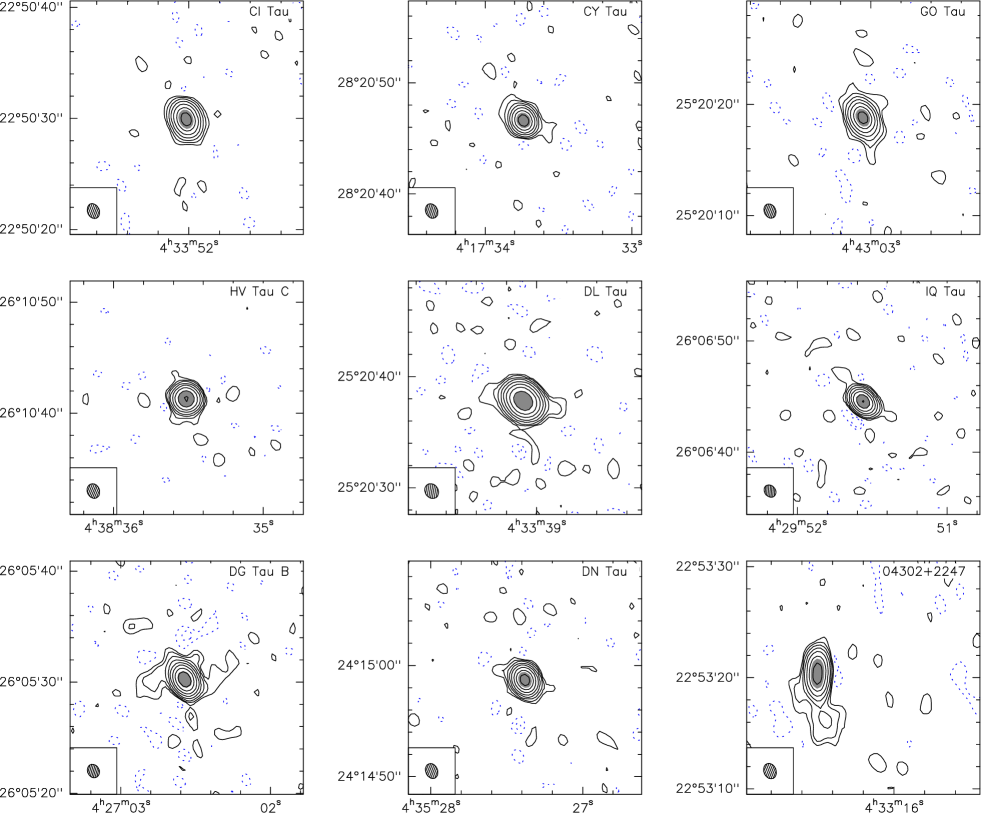
Figure 1: Continuum images for all newly observed sources. Contour levels are logarithmically spaced, by a factor 2: -2 and 2, 4, 8, 16, 32, 64, 128 and 256 $\sigma$. Rms noise (in mJy/beam) and peak signal to noise are: CI Tau 0.6 and 180, CY Tau 0.5 and 190, GO Tau 0.26 and 180, HV Tau 0.12 and 230, DL Tau 0.23 and 550, IQ Tau 0.23 and 270, DG Tau B 0.7 (dynamic range limited) and 450, DN Tau 0.25 and 360, and IRAS04302+2247 0.4 and 180

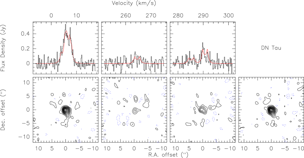
Figure 11: Results for DN Tau. Top: Integrated line flux for CN N=2-1 hyperfine components (histogram) with the best fit profile superimposed (red curve). Bottom: Signal to noise maps for each group of components, and for all observed components (rightmost panel). Contours are in steps of 2 $\sigma$.

For each source, we have two or three data cubes of $128\times 128$ pixels and 460 channels each. Signal is spread over 50 to 100 channels, but the signal to noise per channel is in general rather low (see for example Fig.11). It is hopeless to present the full data cubes. For each source, we present instead two “optimal” quantities. The first quantity is the set of spectra for each (group of) hyperfine component, integrated over the disk area defined below. The second one are images of optimally filtered spectra, as computed for N₂H⁺ by Dutrey et al. (2007). Each channel is multiplied by the intensity of the integrated spectrum predicted by the best fit model. All channels are then summed together: the resulting quantity has the dimension of an intensity squared summed over velocity, and no simple physical interpretation, but gives the signal-to-noise for detecting line emission which matches the model profile. This signal to noise image shows where the emission is located. The process is applied separately for each (group of) hyperfine component, and then globally. The global S/N map serves as a mask to compute the integrated spectra, using a 2 $\sigma$ threshold.

Figure 2: Results for GO Tau. Top: Integrated line flux for CN N=2-1 hyperfine components (histogram) with the best fit profile superimposed (red curve). Bottom: Signal to noise maps for each group of component, and for all observed components (rightmost panel); contour spacing is $2\sigma$.

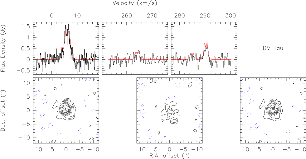
Figure 8: Results for DM Tau. Top: Integrated line flux for CN N=2-1 hyperfine components (histogram) with the best fit profile superimposed (red curve). The spectral resolution for the strongest group of hyperfine components is 0.103 km s^-1. Bottom: Signal to noise maps for the two groups of components, and for all observed components (rightmost panel). Contours are in steps of 2 $\sigma$.

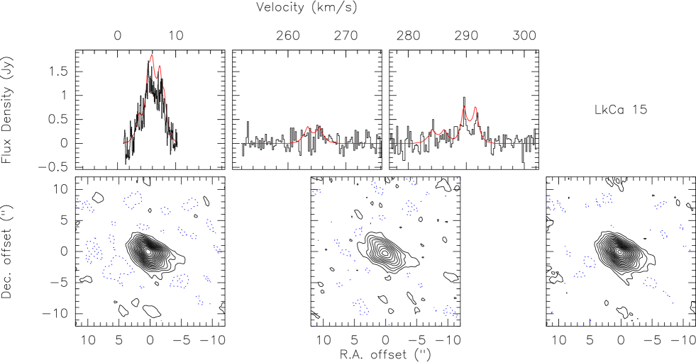
Figure 9: As Fig.8 for LkCa 15.

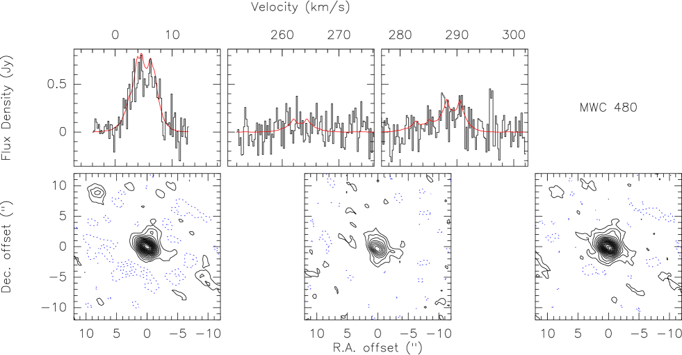
Figure 10: As Fig.8 for MWC 480.

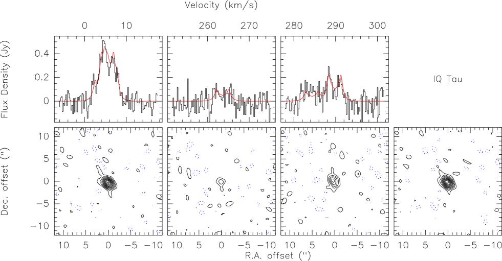
Figure 13: As Fig.11 for IQ Tau.

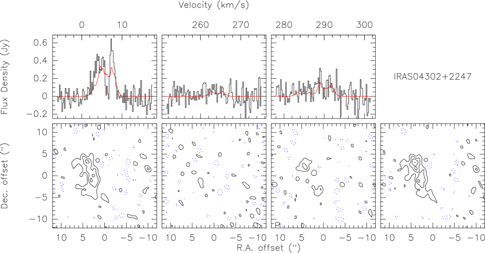
Figure 14: As Fig.11 for IRAS 04302+2247.

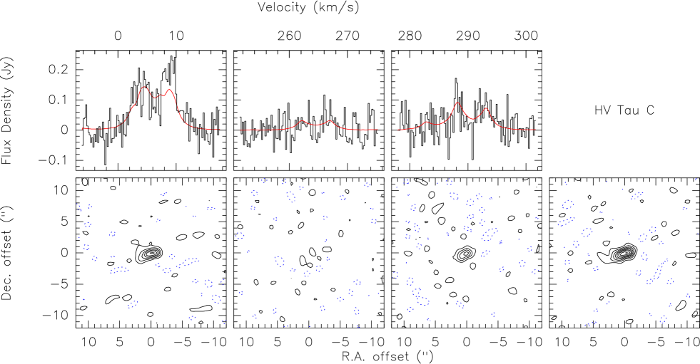
Figure 15: As Fig.11 for HV Tau.

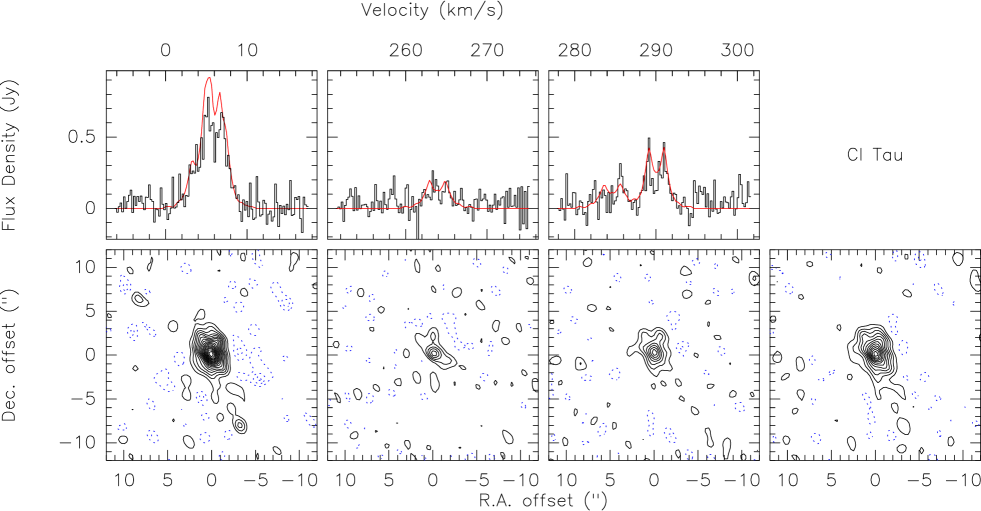
Figure 16: As Fig.11 for CI Tau.

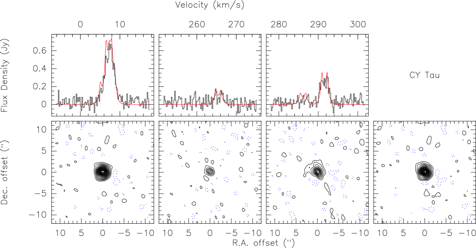
Figure 17: As Fig.11 for CY Tau.

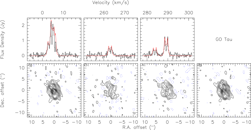
Figure 18: As Fig.11 for GO Tau.

An example of these integrated spectra and signal to noise maps is given in Fig.2. All other sources are shown in Appendix A in Figs.8-18, except for DG Tau B which is discussed in Sect.3.3.4. Unless noted, the spectra have been smoothed to 0.206 $\,{\rm km\,s}^{-1}$ resolution for better clarity. The agreement between the observed line profiles and the best fit results appears sometimes limited, but this is a result of the difficulty to deconvolve low signal to noise data combined with synthesized beams with substantial sidelobes. Under such circumstances, the deconvolution cannot recover the total flux.

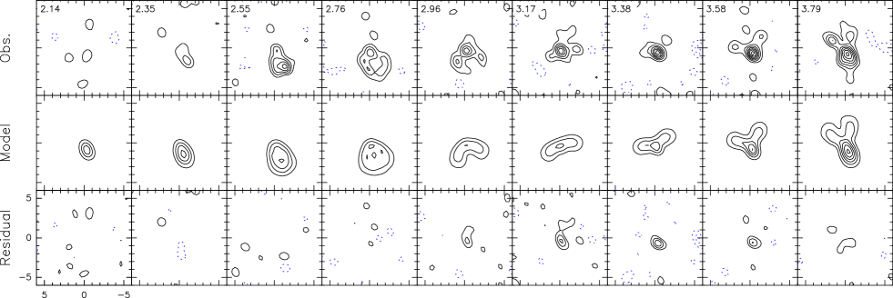
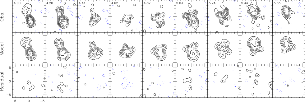
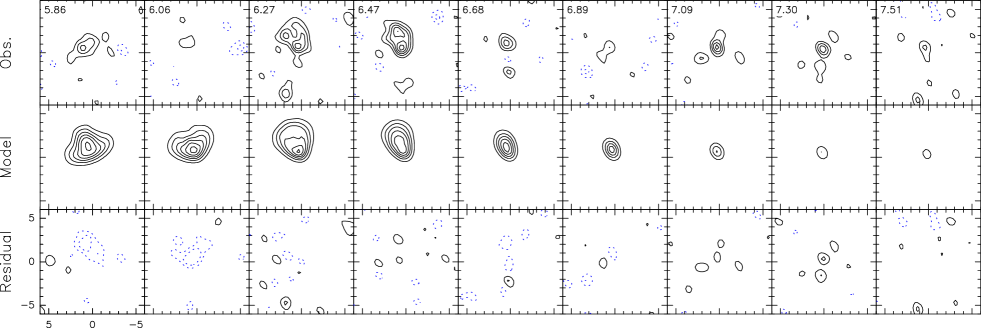
Figure 19: Line channels for GO Tau. For each panel, observations are displayed in the top row, the best fit model in the middle row and the residuals in the bottom row. Channels are ordered by increasing velocities (see upper left corner of each panel) from left to right and top to bottom. Contour spacing is 40 mJy/beam, or 2 $\sigma$. The unusual spatial distribution is due to the three hyperfine components. The emission is essentially that of 3 Keplerian disks with systemic velocities 3.37, 4.87, and 5.66 km.s^-1 and relative intensities 1, 2.67 and 1.68 respectively.

All sources show clear evidence for rotation, but illustrating the velocity gradient is not straightforward because of the multiple (and for the strongest, blended) hyperfine components (see Fig.19). We show in Fig.3 the first moment map derived from the isolated hfs component near 290 km s^-1 in GO Tau. The fitting procedure, which takes all hyperfine components into account, retrieves the related information (orientation, velocity field and inclination) with much better precision.

Relevant parameters from the fit results are presented in Table 4. To illustrate the fit quality, we present in Appendix (Fig.19) channel maps for the strongest group of hyperfine components in GO Tau: observations, best model and residuals. On average, there is no systematic dependency of the residuals with velocities, and channels with strong emission have similar residuals than channels without. Although a few channels have some systematic residuals, this can be ascribed by the limitations of our disk model, such as the assumption of power law for the CN surface density, and should not affect the derived velocity field. For all other sources, we obtained significantly less signal to noise than for GO Tau, and noise is the limiting factor in the velocity field derivation.

A comparison between geometric parameters derived from CN and dust emission is given in Table 2. The stellar mass is derived from the Keplerian rotation of the disks. Because the maps provide only an angular scale the derived masses are proportional to the distance to the star. The masses listed in Table 4 are given at the star-forming region’s (SFR) average distance, 140 pc (Kenyon et al. 1994).

Table 4: Disk and Star parameters derived from CN

Source	V100	i	$R_{\mathrm{out}}$	M∗	$\delta v$
name	(km s-1)	(∘)	AU	($M_{\odot}$)
DM Tau	2.31 $\pm$ 0.17	-30.9 $\pm$ 2.9	641 $\pm$ 19	0.60 $\pm$ 0.09	0.1 $\pm$ 1.5
MWC 480	4.03 $\pm$ 0.41	36.3 $\pm$ 2.5	539 $\pm$ 39	1.83 $\pm$ 0.37	-2.2 $\pm$ 2.0
LkCa 15	3.11 $\pm$ 0.10	47.0 $\pm$ 1.3	567 $\pm$ 39	1.09 $\pm$ 0.07	0.0 $\pm$ 2.4
CI Tau	2.67 $\pm$ 0.03	51.0 $\pm$ 0.9	520 $\pm$ 13	0.80 $\pm$ 0.02	-2.7 $\pm$ 2.0
CY Tau	2.36 $\pm$ 0.12	24.0 $\pm$ 2.0	295 $\pm$ 11	0.63 $\pm$ 0.05	1.7 $\pm$ 1.7
GO Tau	2.07 $\pm$ 0.01	54.5 $\pm$ 0.5	587 $\pm$ 55	0.48 $\pm$ 0.01	4.0 $\pm$ 2.0
HV Tau C	3.76 $\pm$ 0.10	89.1 $\pm$ 3.0	256 $\pm$ 51	1.59 $\pm$ 0.08	-0.0 $\pm$ 2.9
DL Tau	2.83 $\pm$ 0.04	44.1 $\pm$ 2.6	463 $\pm$ 6	0.91 $\pm$ 0.02	1.9 $\pm$ 1.1
IQ Tau	2.64 $\pm$ 0.02	56.3 $\pm$ 3.9	225 $\pm$ 21	0.79 $\pm$ 0.02	-0.3 $\pm$ 4.9
DN Tau	2.91 $\pm$ 0.25	29.2 $\pm$ 3.0	241 $\pm$ 7	0.95 $\pm$ 0.16	-0.6 $\pm$ 1.8
04302+2247	4.18 $\pm$ 0.09	58.9 $\pm$ 2.1	750 $\pm$ 56	1.97 $\pm$ 0.08	-0.4 $\pm$ 2.3

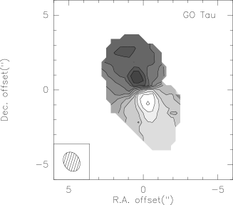
Figure 3: Velocity gradient for GO Tau. Contour spacing is 0.2 km s^-1.

3.1 CN as a dynamical mass tracer

A first important result from this study is an unambiguous confirmation that CN is essentially unaffected by contamination from the molecular clouds. The full kinematic pattern of the disk is visible, leading to accurate determination of the systemic velocity. However, the disk interpretation does not apply for the two embedded (presumably younger) objects DG Tau B and IRAS04302+2247.

A second essential result from Table 4 is that all sources appear in Keplerian rotation. The weighted mean deviation from the Keplerian exponent $v=0.50+0.01\delta v$ is $\delta v=0.5\pm 0.6$. Thus, we can safely interpret the rotation pattern as being driven by a central mass.

The third result is the good agreement between geometric parameters (position angle and inclination) derived from other tracers. This is shown for CI Tau, DL Tau and CY Tau in Table 3. This agreement is important, because the geometric parameters are affected by different systematic effects due to calibration uncertainties. For continuum data, phase errors (for the high resolution data of Guilloteau et al. 2011) or amplitude errors (for our self-calibrated data) can bias the result beyond the thermal noise. For spectral line data, the orientation is defined by the velocity gradient, and thus depends on the phase bandpass calibration.

Finally, in previously studied isolated sources, the systemic velocity derived from CN is (within the noise induced uncertainties) in agreement with values derived from other molecular transitions (see Piétu et al. 2007, for DM Tau, LkCa 15 and MWC 480).

We thus conclude that, within the uncertainties of the measurements reported here, CN is a good tracer of the dynamical mass. This dynamical mass may however overestimate the stellar mass: given the angular scale of the study, it includes any contribution from any compact ($<20-30$ AU radius) disk that may surround the star.

3.2 The vertical distribution of CN

In our analysis, CN is assumed to be homogeneously distributed in the vertical direction, i.e. to be distributed vertically following a gaussian whose characteristic size is the disk scale height. The scale height was initially arbitrarily fixed to $H_{100}=16.5$ AU and $h=-1.25$ (mildly flared disk). However, we expect CN to be located at the top of the molecular layer, between the highly irradiated surface layer where molecules are photo-dissociated and the colder disk plane where molecules condense on grains. Although this expected distribution has so far not been confirmed by imaging studies, and even faces some difficulty when considering the expected temperature in this molecular layer (Chapillon et al. 2012), it is important to evaluate if this can affect the derived disk inclination and hence, the stellar mass measurement.

We did that in 3 steps. First, we explored different disk thickness. This did not significantly affect the derived dynamical mass. Second, we treated the scale height as a free parameter. We found in general larger values for $H_{100}$, and flatter disks $h\approx-1.0$, which is consistent with the molecules being closer to the disk surface. However, the number of free parameters becomes large, and the fits sometimes converge towards unrealistic solutions (e.g. very large $H_{100}$ and $h>-1.0$). Third, we used the method described by Guilloteau et al. (2012) for the analysis of CS in DM Tau. We assumed CN molecules to be absent at any point where the H₂ column disk towards the disk surface $\Sigma_{o}(r,z)$ is larger than a given value, $\Sigma_{d}$. $\Sigma_{o}(r,z)$ density is computed using the prescribed scale height ($H_{100}=16.5$ AU and $h=-1.25$), and with the surface density profile corresponding to the best fit viscous disk model to the 226 GHz continuum data:

$$\Sigma_{g}(r)=\Sigma_{0}\left(\frac{r}{R_{0}}\right)^{-\gamma}\exp\left(-(r/R_{c})^{2-\gamma}\right).$$ (2)

Despite the much more limited angular resolution of the new data, we reached a similar precision on $\gamma$ and $R_{c}$ as Guilloteau et al. (2011), thanks to the higher sensitivity and lower phase noise due to self-calibration. Furthermore, the values found for $\gamma$ and $R_{c}$ were within the errors equal to those measured by Guilloteau et al. (2011). We varied the depletion scale height $\Sigma_{d}$ between $10^{21}$ and $10^{24}$ cm^-2. The most extreme values provided significantly worse fit to the data, with a best fit $\Sigma_{d}$ around $10^{23}$ found for most sources. The derived disk inclinations and dynamical masses only change by small amounts as a function of $\Sigma_{d}$: less than $\sim\sigma/3$ over the acceptable range of values for $\Sigma_{d}$, and even at most about $1\sigma$ for more extreme values.

We thus conclude that the uncertainties in the spatial distribution of CN due to our limited knowledge of the disk structure and chemistry do not affect the reliability of the CN N=2-1 transition as a tracer of the dynamical mass.

3.3 Special sources

We derived accurate dynamical masses for most sources in our sample. However, a few sources are peculiar in this respect, because of unfavorable inclination and orientation, evolutionary status or multiplicity. We discuss here these sources which we omit in further analysis.

3.3.1 HV Tau

HV Tau is a triple system: AB is a close visual binary with angular separation around 70 mas (Simon et al. 1996), and HV Tau C is a much fainter T Tauri star located 4^′′ NE of AB. A nearly edge-on compact dust disk surrounds HV Tau C (Monin & Bouvier 2000), but AB shows no IR excess and no sign of accretion (White & Ghez 2001). The system was modeled in detail by Duchêne et al. (2010), who showed that mm-emission only comes from the HV Tau C circumstellar disk, which also exhibit ¹²CO emission compatible with Keplerian rotation, although only the line wings are clearly visible.

CN emission was detected using the IRAM 30-m by Guilloteau et al. (2013), who attributed it to HV Tau C based on the previous non-detection of any circumstellar material around AB by Duchêne et al. (2010). Our images confirm this association. The derived dynamical mass, $\sim 1.6M_{\odot}$, is much larger than suggested by apparent spectral type (K6, White & Hillenbrand 2004). Given the system complexity, a more complete study of the HV Tau multiple system will be presented in a separate paper.

With IQ Tau, HV Tau C is another good example of disk detection through CN while CO emission is heavily contaminated by the molecular cloud. Note that both stars are close to each other, and affected by the same molecular cloud. The higher inclination of HV Tau C allows the line wings to remain visible in CO.

3.3.2 CY Tau

CY Tau and DN Tau are the two sources which combine a small (280 AU) disk with a low inclination (25-30^∘). The DN Tau disk is favorably oriented with respect to the synthesized beam, allowing the inclination to be precisely measured. On the contrary, for CY Tau, the synthesized beam major axis is within $30^{\circ}$ of the disk rotation axis, so that the limited angular resolution in this direction makes the inclination, and consequently the deprojected rotation velocity, rather uncertain. Without self calibration for CN, the $\chi^{2}$ curve as a function of inclination for CY Tau has two minima, at $\simeq 21^{\circ}$ and $\simeq 30^{\circ}$, separated by about $3\sigma$. After application of the self-calibration solution from the continuum data, this CN $\chi^{2}$ curve now exhibits a single minimum, indicating an inclination of $\simeq 24\pm 2^{\circ}$. However, low inclinations are not strictly excluded, and the only safe conclusion is $i<28^{\circ}$ at the $3\sigma$ level, which implies $M_{*}>0.45M_{\odot}$ from CN only. From the CN $\chi^{2}$ curve, we derive $M_{*}=0.63^{+0.11}_{-0.06}M_{\odot}$. However, using all other available measurements, the weighted mean of the inclinations is $27\pm 2^{\circ}$, and the weighted $v\sin{i}=0.95\pm 0.04\,{\rm km\,s}^{-1}$, which suggest a somewhat lower value for the most likely mass, $\sim 0.51M_{\odot}$.

In our nominal solution from CN, we find an orientation which agree with previous higher resolution measurements made from continuum and CO (Guilloteau et al. 2011), see Table 3. The orientation derived from the (self-calibrated) continuum is different (although marginally, i.e. at the $2\sigma$ level, the errors being large). Such a difference can be due to inaccuracies in the amplitude calibration as a function of time (and hence hour angle). Similar calibration inaccuracies cannot significantly affect other disks, since their axis ratio is much larger than for CY Tau (or better constrained because of a more favorable orientation in the case of DN Tau).

3.3.3 The Butterfly star, IRAS 04302+2247

In this embedded source, CN is clearly not peaking towards the continuum (see Fig.4), and does not originate from the inner disk traced by dust and CO isotopologues. Although the morphology could be the trace of asymmetric emission from the envelope surrounding the central disk, we also fitted CN emission by a flared, rotating disk. The derived centroid, orientation, and inclination differ strongly from those of the continuum disk, reflecting the apparent asymmetry. We find an inner radius around 150 AU, similar to the large grains disk size found by Gräfe et al. (2013), thus indicating that CN is not present in the dense disk, but only in the outer envelope. Despite this different morphology, the rotation pattern still appears nicely Keplerian, and the derived total mass, $1.9M_{\odot}$, is consistent with the sum of the star ($1.7M_{\odot}$, Dutrey et al.  2014, in prep.) and disk mass.

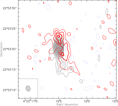
Figure 4: Superposition of the CN N=2-1 emission (in red contours) over the continuum emission (in grey scale) in IRAS04302+2247. Contour levels are 2,4,6,8 $\sigma$ for CN, and 2, 4, 8, 16 and 32 $\sigma$ for the 1.4 mm continuum emission.

The continuum emission clearly reveals a weak, resolved, secondary source $4^{\prime\prime}$ south of the main disk (at PA 171^∘), with a total flux density of 12 mJy. The main disk has a flux of 138 mJy. IRAS 04302+2247 may actually be the progenitor of a binary (or higher multiplicity) system.

3.3.4 DG Tau B

DG Tau B is another embedded object, with a powerful, one-sided, molecular outflow (Mitchell et al. 1997). The rather low signal to noise limits our ability to interpret the CN distribution. However, the CN emission is not centered on the strong continuum emission. On the contrary, we detect absorption towards the continuum source, and emission predominantly east of the continuum peak, see Fig.5. The absorption profile is very uncertain, but could be due to a single narrow component at $V_{\mathrm{LSR}}\simeq 6.2\,{\rm km\,s}^{-1}$, the hyperfine structure leading to the impression of two velocity features. The cloud velocity towards DG Tau B is $6.44\,{\rm km\,s}^{-1}$ from C¹⁷O measurements (Guilloteau et al. 2013). The peak continuum flux is 220 mJy/beam, or about 3.7 K, and the absorption dip has a depth of about 60 mJy/beam. Assuming the absorbing material fills the synthesized beam, this implies an upper limit on the excitation temperature of 7 K (taking into account the deviations from the Rayleigh Jeans approximation), obtained for optically thick absorbing medium. This is consistent with the expected temperatures in the surrounding dense cloud.

On the contrary, the emission has a much larger linewidth, of order 3-4 $\,{\rm km\,s}^{-1}$. The integrated line flux is $\sim 0.6$Jy$\,{\rm km\,s}^{-1}$, about 50 % of the flux detected by the 30-m, which suggests that some low level emission has not been recovered properly .

Figure 5: Top: (continuum subtracted) integrated emission from CN N=2-1 main group of hyperfine components in DG Tau B. Note the negative contours towards the continuum source at (0,0). Middle: CN N=2-1 spectrum toward the continuum source. Bottom: integrated flux density over the emission region.

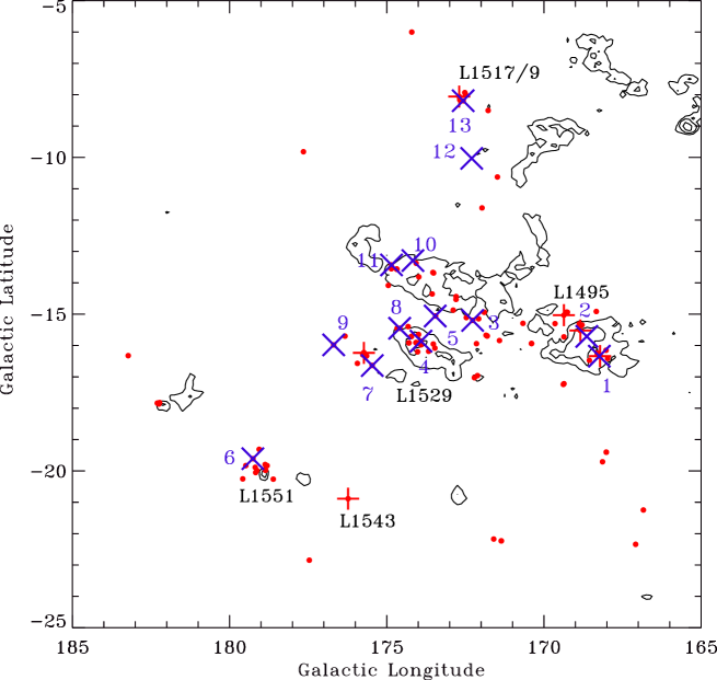
Figure 6: Location of the observed stars in the Taurus Auriga region. The contours are low lying levels of CO integrated intensity from the Dame et al. (2001) survey. The red dots are stars in common between Ducourant et al. (2005) and Kenyon et al. (2008) master list of PMS stars in Taurus. The red crosses show the stars with precise distances (VLBA or VB+SB2) The blue crosses show the stars with masses measured by disk rotation.

4 Discussion: Implications for stellar evolution models

Table 5: Dynamical masses for single stars

	Name	SpType	Teff	$L_{*}$	$M_{*}$	Comments
Number			(K)	$L_{\odot}$	$M_{\odot}$	& References
1	CW Tau	K3	$4840^{+200}_{-220}$	$2.42\pm 1.40$	$0.69\pm 0.14$	M1, L0, L1495
2	CY Tau	M1	$3615\pm 65$	$0.40\pm 0.09$	$0.63\pm 0.05$	M0, L0, L1495
3	IQ Tau	M0.5	$3765\pm 85$	$0.81\pm 0.26$	$0.79\pm 0.02$	M0, L0
4	Haro 6-13	M0	$3850^{+200}_{-170}$	$0.69\pm 0.22$	$1.00\pm 0.15$	M4, L0. L1529
5	DL Tau	K7	$4050^{+150}_{-200}$	$0.74\pm 0.38$	$0.91\pm 0.02$	M0, L0
6	DM Tau	M1	$3680^{+170}_{-130}$	$0.23\pm 0.02$	$0.53\pm 0.02$	M2, L0, L1551
7	CI Tau	K7	$4050^{+150}_{-200}$	$0.93\pm 0.35$	$0.80\pm 0.02$	M0, L0, L1529
8	DN Tau	M0	$3850^{+200}_{-170}$	$0.79\pm 0.16$	$0.95\pm 0.16$	M0, L0, L1529
9	LkCa 15	K5	$4450^{+170}_{-250}$	$0.81\pm 0.21$	$1.01\pm 0.03$	M2, L0
10	Haro 6-33	M0.5	$3765^{+115}_{-85}$	0.76	$0.5\pm 0.1$	M4, L1
11	GO Tau	M0	$3850^{+200}_{-170}$	$0.29\pm 0.09$	$0.48\pm 0.01$	M0, L0
12	DS Tau	K5	$4450^{+170}_{-250}$	$0.76\pm 0.34$	$0.68\pm 0.12$	M1, L0
13	GM Aur	K3	$4850^{+200}_{-220}$	$1.23\pm 0.32$	$1.00\pm 0.02$	M3, L0, L1517/9

Comparison of the measured masses with theoretical evolutionary tracks is best made on a modified HRD in which the distance-independent quantity $L/M_{*}^{2}$ is plotted $vs\leavevmode\nobreak\ T_{\mathrm{eff}}$ (Simon et al. 2000). Table 5 lists the stellar parameters of the stars we consider for a comparison with models of PMS stellar evolution. For completeness, Table 5 also lists the masses for several of stars that were reported previously. Figure 6 shows the locations of these stars within the SFR. Of the stars in Table 4, Table 5 does not include MWC 480, HV Tau C, and 04302+2247. Piétu et al. (2007) have already carefully considered MWC 480 on the modified HRD. We will discuss the multiple system HV Tau and its masses in a forthcoming paper (Guilloteau et al 2014, in prep.), and 04302+2247 is a Class I YSO with inadequately known stellar parameters (Gräfe et al. 2013). All spectral types (col. 3), effective temperatures, $T_{\mathrm{eff}}$ (col. 4), and luminosities (col. 5) are from Andrews et al. (2013) except for Haro 6-33 which is from White & Hillenbrand (2004). We assumed $T_{\mathrm{eff}}$ uncertainties corresponding to $\pm 1$  spectral type and used the spectral type-$T_{\mathrm{eff}}$ look-up table in Pecaut & Mamajek (2013). To calculate uncertainties in $L/M_{*}^{2}$ we propagated the uncertainties in L and M according to the usual procedure for the uncertainty of a ratio when one of the variables is squared.

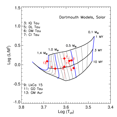
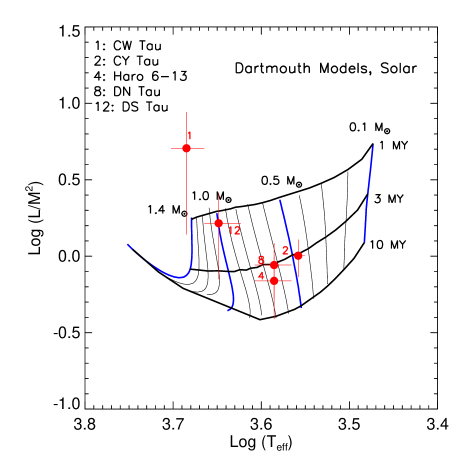
Figure 7: Stars on the modified, distance-independent, HR diagram $L/M^{2}vs$ T_eff from Dotter et al. (2008) evolutionary tracks. Left: stars with dynamical masses accurate to $<5\%$, right: other stars.

Table 6: Comparison of best Masses with tracks

#	Star	Dynamical	Agreement & Evolutionary Track Mass range
		Mass	BCAH	SDF	Pisa	Dartmouth
3.	IQ Tau	$0.79\pm 0.02$	F  0.65-0.70	F  0.45-0.70	F  0.48-0.72	P  0.50-0.60
5.	DL Tau	$0.91\pm 0.02$	E  0.72-0.92	E  0.60-0.92	F  0.62-0.88	F  0.68-0.88
6.	DM Tau	$0.53\pm 0.02$	E  0.50-0.70	E  0.35-0.59	E  0.43-0.62	E  0.44-0.62
7.	CI Tau	$0.80\pm 0.02$	E  0.70-0.88	E  0.58-0.90	E  0.60-0.82	E  0.59-0.80
9.	LkCa 15	$1.01\pm 0.03$	E  0.92-1.30	E  0.95-1.30	E  0.90-1.25	E  0.92-1.30
11.	GO Tau	$0.48\pm 0.01$	P  0.70-0.92	E  0.45-0.75	F  0.52-0.82	E  0.48-0.70
13.	GM Aur	$1.00\pm 0.02$	P  1.35-?	P  1.51-?	P  1.30-?	P  1.20-?

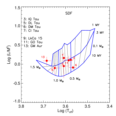
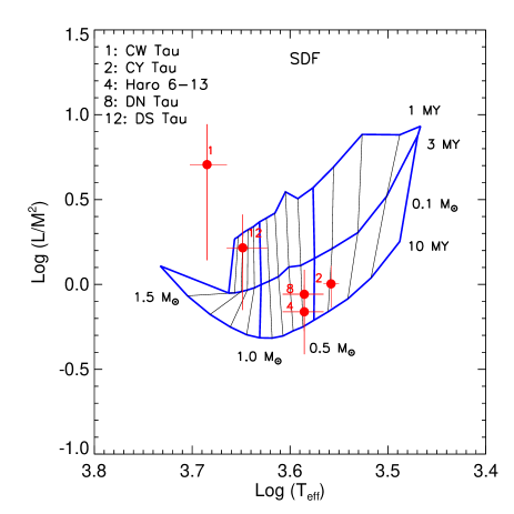
Figure 21: As for Fig.20, but for the Siess et al. (2000) tracks.

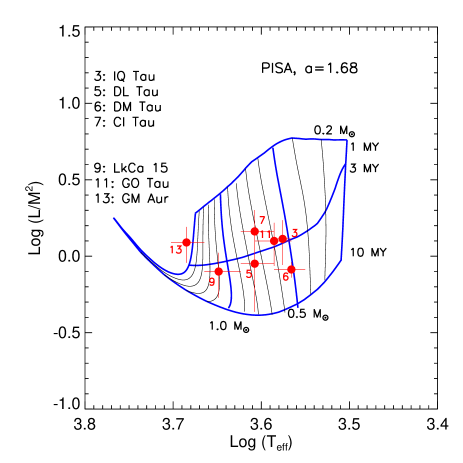
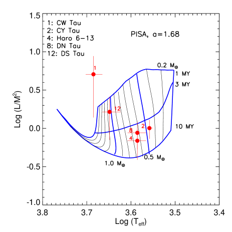
Figure 22: As for Fig.20, but for the Tognelli et al. (2011) tracks.

For stars in Table 5 with mass uncertainties less than or equal to $\pm 5\%$, Fig.7a plots their $L/M_{*}^{2}$ vs $T_{\mathrm{eff}}$ on a modified HRD using the evolutionary tracks calculated by Dotter et al. (2008, Dartmouth). Figure 7b is a similar plot for stars with mass precisions worse than $\pm 5\%$. Figure 7b does not include Haro 6-33 because the uncertainty of its luminosity is not available. Figs.20-22 in Appendix C show similar plots for the evolutionary tracks of Baraffe et al. (1998, BCAH), Siess et al. (2000, SDF), and Tognelli et al. (2011, Pisa). The numbering of the stars follows that of Table 5.

Three features are apparent in all the modified HRD plots:

1. No stars with mass below $\sim 0.5M_{\odot}$ appear. Mass measurement by the circumstellar disk technique of lower mass stars in Taurus requires higher sensitivity, presumably because their disks are less massive (e.g. Schaefer et al. 2009; Andrews et al. 2013) but also much smaller (Piétu et al. 2014).

2. $T_{\mathrm{eff}}$ uncertainties severely compromise the comparisons with the tracks because most uncertainties span tracks separated by more than $0.1M_{\odot}$.

3. Uncertainties in $L/M_{*}^{2}$ affect comparisons with evolutionary tracks very little because, at the ages displayed, the tracks are nearly parallel to the $L/M_{*}^{2}$ axis. However, uncertainties in $L/M_{*}^{2}$ can affect the age estimate.

Table 6 summarizes, qualitatively, a comparison of the best masses with the 4 theoretical tracks. Columns 1 and 2 identify the stars and column 3 repeats, for convenience, their measured dynamical masses at 140 pc distance. Columns 4-7 give the mass range corresponding to the $\pm 1\sigma$ uncertainties of the ($T_{eff},L/M_{*}^{2}$) values. Table 6 indicates that the measured masses of DM Tau, CI Tau, and LkCa 15 (0.53, 0.80, and $1.01M_{\odot}$, respectively) are in agreement with all 4 sets of tracks if they are actually at the fiducial distance 140 pc. However, IQ Tau with a measured mass indistinguishable from that of CI Tau, and GM Aur with a measured mass indistinguishable from that of LkCa 15, are inconsistent with their nominal mass tracks $0.80M_{\odot}$ and $1.00M_{\odot}$, respectively. Two reasons are likely. Their published spectral types may not provide an accurate indication of their $T_{\mathrm{eff}}$. Also, their distances may be greater or less than 140 pc which would not affect their $L/M_{*}^{2}$ values but would change their mass derived from the angular measure of their disk rotation. For example, Fig.6 shows that the position of GM Aur in the L1517/19 region is close to NTTS 045251+3016 at distance $158.7\pm 3.9$ pc (Simon et al. 2013). If this distance applies to GM Aur, its mass would become (158.7/140) times greater, i.e. $1.13\pm 0.02M_{\odot}$, decreasing the discrepancy with respect to the $1.1M_{\odot}$ theoretical track but still more than $\sim 1\sigma$ too high with respect to all the $1.1M_{\odot}$ tracks. Fig.6 also shows that the position of CI Tau in the L1529 region is close to HP Tau G2 for which Torres et al. (2009) measured the precise distance $161.2\pm 0.9$ pc. At this distance the measured mass of CI Tau would be (161.2/140) times greater or $0.92\pm 0.02M_{\odot}$. If this were its actual mass, the quality of consistency with the Dartmouth and Pisa evolutionary would be degraded. It seems reasonable to conclude that a definitive comparison of the measured masses with the available theoretical evolutionary tracks should await a more accurate determination of effective temperatures of the target stars, mass measurements of stars with masses below $0.5M_{\odot}$, and accurate distances to all.

For the stars with the most precise mass measurements, Table 7 summarizes the ages indicated by their locations on the modified HRDs. All 4 theoretical calculations indicate the stars are younger than 10 Myr, and that a representative age for most of the stars is between 2 and 4 Myr, consistent with prior estimates (e.g. Kenyon et al. 2008). Improved values of stellar parameters will yield more accurate age estimates.

In conclusion, the reliability of these comparisons of the measured masses with the theoretical tracks is compromised by the uncertainties on the effective temperatures and distances. Also, a definitive assessment of the theoretical evolutionary tracks must await mass measurements of stars with masses below $0.5M_{\odot}$. We look ahead to GAIA to provide precise distances to stars in the Taurus star forming region and have started measurements that we hope will improve the determinations of $T_{\mathrm{eff}}$ and will extend mass measurements to masses smaller than those presented in this paper.

Table 7: Approximate ages (Myr)

#	Star	Evolutionary Tracks
		BCAH	SDF	Pisa	Dartmouth
3.	IQ Tau	2	3	3	2
5.	DL Tau	3	4	4	3
6.	DM Tau	5	8	5	3.5
7.	CI Tau	1.5	2.5	2.5	1.5
9.	LkCa 15	3	4	4	3
11.	GO Tau	2	4	3	3
13.	GM Aur	2	2	2	1.5

5 Conclusion

We have analyzed $\sim 1.2^{\prime\prime}$ arcsecond resolution observations of the CN N=2-1 line in a sample of T Tauri stars, and performed a comparison with $\sim 0.6^{\prime\prime}$ resolution data obtained in ¹²CO for several sources. The results show that the CN transition is a good, sensitive, contamination free, dynamical mass tracer for stars in the M1 - A4 spectral type range that are surrounded by disks larger than about 250 AU. The striking ability of CN to overcome the contamination problem is best shown by the detection of the disk in IQ Tau that escaped detection in CO at similar angular resolution.

The largest uncertainty in the mass derivation comes from the determination of the inclination, although the impact is small for sources with $i>45^{\circ}$. This uncertainty can be reduced by higher angular observations, at the expense of more observing time. Another pending problem is that the more embedded, presumably younger, objects like DG Tau-B or IRAS04302+2247, have more complex structure and CN does not appear to be a very good disk tracer in these sources.

We used the derived dynamical masses in conjunction with similar measurements performed using other tracers to compare with the evolutionary tracks. Agreement of the measured masses with the evolutionary tracks is quite good. The discrepancies are most likely attributable to inaccurate effective temperatures and, to a lesser extent, distances different from the 140 pc average value. We hope to remove some of these discrepancies and to extend the mass measurements below $0.5M_{\odot}$ (spectral type earlier than M2) where the differences among the theoretical calculations are the greatest.

Appendix A CN images and profiles

Figure 12: As Fig.11 for DL Tau.

Appendix B Fit residuals

Appendix C Evolutionary Tracks

To compare the masses we have measured to different evolutionary models, we show in Fig.20-22 the position of the stars with accurate masses on modified HR diagram for the Baraffe et al. (1998, BCAH), the Siess et al. (2000) and the Tognelli et al. (2011, PISA) tracks; see also Fig.7 for the Dartmouth (Dotter et al. 2008) tracks. Taken together, the four different models differ the most with respect to each other at masses less than $0.5M_{\odot}$ and have different evolutionary time scales for all masses at ages less than 5 Myr.

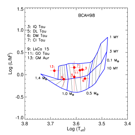
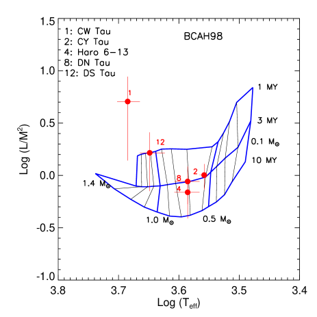
Figure 20: Stars on the modified, distance-independent, HR diagram $L/M^{2}vs$ T_eff for the Baraffe et al. (1998) tracks. Stars with dynamical mass precisions measured to better than 5% appear in the left panel and stars with lower precions appear in the right panel.