Maximum population transfer in a periodically driven quantum system

Abstract

We study the dynamics of a two-level quantum system under the influence of sinusoidal driving in the intermediate frequency regime. Analyzing the Floquet quasienergy spectrum, we find combinations of the field parameters for which population transfer is optimal and takes place through a series of well defined steps of fixed duration. We also show how the corresponding evolution operator can be approximated at all times by a very simple analytical expression. We propose this model as being specially suitable for treating periodic driving at avoided crossings found in complex multi-level systems, and thus show a relevant application of our results to designing a control protocol in a realistic molecular model.

I Introduction

Understanding the coherent manipulation of quantum systems using time-dependent interacting fields is a goal of primary interest in many different areas, including chemical reactivity bib:chem , nanotechnology bib:nano , and quantum information processing bib:qc . To this end, simple analytically solvable two-level systems (TLS) are often used since they can efficiently describe the dynamics. One popular choice is the Landau-Zener model bib:zener , in which the driving field is assumed to vary linearly with time. Nonetheless, in many experimental situations sinusoidal, time-periodic control fields are easier to produce and manipulate, and are thus the preferred option. Beyond the well-known Rabi model (which accounts for the weak driving case), many approaches have been used in the literature to describe various non-trivial limits of this type of systems bib:floquet ; bib:nori ; bib:wu ; bib:dassarma .

A striking phenomenon induced by time-periodic fields is the so-called coherent destruction of tunneling (CDT), first predicted by Grossmann et al. bib:grossman and then observed experimentally bib:cdtexp1 . A particle in a symmetric double-well potential usually oscillates back and forth, if initially localized in one of the wells. However, if the depth of the wells oscillates in time, the tunneling rate may dramatically change. Actually, for certain combinations of the driving parameters, the rate vanishes, resulting in an effective localization of the particle in the initial well. As previously shown bib:grossman ; bib:deg , this behavior takes place only when some Floquet quasienergies are degenerate.

In this work, we show that the Floquet spectrum of a TLS under a sinusoidal driving in the regime of intermediate frequencies ($\omega\simeq\Delta$, being $\omega$ the driving frequency and $\Delta$ the characteristic frequency of the system bib:hbarra ) shows a second kind of “special points”, defined by the condition that the quasienergy separation is a local maximum, where: (i) population inversion is achieved after a time interval that only depends on the quasienergy difference; (ii) the evolution of the populations happens through a series of well-defined steps of fixed duration, in which the probability remains approximately constant, and (iii) the full time-dependent evolution operator $U(t)$ can be obtained in a very simple analytical form, which provides a clear physical interpretation of (ii).

Finally, taking into account the general validity of this two-level model, we study at what extent the results we obtain can be applied to multi-level systems which are periodically driven at an avoided crossings (AC). By designing of a control protocol in a realistic model for the LiNC$\rightleftharpoons$LiCN isomerization bib:brocks ; bib:murgida , we find that the intermediate frequency regime is specially suitable for such complex systems.

This paper is organized as follows. In Sec. II we present the model system, enumerate the main results of the well-known high frequency regime and present the basics of the Floquet formalism. We then turn to the intermediate frequency regime, where we show that the dynamics of the system changes considerably, showing a remarkably regular behavior for certain values of the driving field amplitude. In Sec. III we ellaborate on the analysis and interpretation of these results, and develop a very simple Bloch sphere model wich allows us to get an analytical solution for the evolution operator. Finally, in Sec. IV we describe the LiCN/LiNC molecular system and propose a control protocol suitable for achieving an isomerization reaction. Sec. V contains some concluding remarks.

II Periodically driven two-level systems

We consider a hamiltonian of the form

$$H(t)=\frac{\Delta}{2}\sigma_{x}+\varepsilon(t)\sigma_{z},$$ (1)

where $\sigma_{x}$ and $\sigma_{z}$ are the usual Pauli operators. The instantaneous eigenvalues of $H$ as a function of the control parameter $\varepsilon$ show the usual avoided crossing (AC) structure, reaching a minimal separation of $\Delta$ at $\varepsilon=0$. We consider the driving field to be $\varepsilon(t)=A\>\mathrm{cos}\left(\omega t\right)$, and define $T=2\pi/\omega$ as the period of $H(t)$. When dealing with this type of systems, it is customary to factorize the evolution operator as $U(t)=U_{1}(t)\>U_{2}(t)$, where $U_{1}(t)=\mathrm{exp}\left[-i\>\gamma_{z}(t)\>\sigma_{z}/2\right]$ can be regarded as a transformation to a rotating frame, since $\gamma_{z}(t)=2\int\varepsilon(\tau)\>d\tau=(2A/\omega)\mathrm{sin}\left(\omega t\right)$. The remaining factor is obtained by the transformed Schrödinger equation $i\dot{U_{2}}(t)=H_{2}(t)\>U_{2}(t)$, where $H_{2}(t)=U_{1}^{\dagger}HU_{1}$ as

$$H_{2}(t)=\frac{\Delta}{2}\left\{\mathrm{cos}\left[\gamma_{z}(t)\right]\sigma_{x}+\mathrm{sin}\left[\gamma_{z}(t)\right]\sigma_{y}\right\}$$ (2)

The time dependence in this expression can be averaged out over one period of the driving field in the high frequency regime, i.e. $\omega\gg\Delta$, using the rotating wave approximation (RWA) bib:nori ; bib:deg . This gives $U_{2}(t)=\mathrm{exp}\left(-i\frac{\Delta^{\prime}}{2}t\>\sigma_{x}\right)$, with $\Delta^{\prime}=\Delta J_{0}\left(2A/\omega\right)$, being $J_{0}$ a Bessel function. For the values of $2A/\omega$ corresponding to the zeros of $J_{0}$, the evolution operator $U(t)$ is diagonal in the $\sigma_{z}$ basis set, $\left\{\left|0\right>,\left|1\right>\right\}$, which explains the occurrence of the CDT phenomenon. For any other value of the amplitude $A$ the population inversion between these states takes place in a finite lapse of time, given by

$$T_{F}=\frac{\pi}{\Delta^{\prime}}.\\$$ (3)

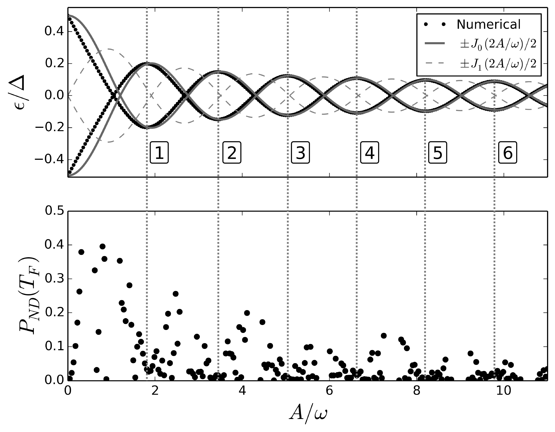
Figure 1: Top: Quasinergy spectrum for the two level hamiltonian of eq. (1) as a function of $A/\omega$. The boxed numbers $n=1,2,\ldots$ label the points of the spectrum in which the quasienergy separation is locally maximal. On top, we plot the analytical expression (4). Bottom: Non decay probability $P_{ND}$ at time $T_{F}$, defined by eq. (3), calculated by numerical simulations of the system prepared in the initial state $\left|0\right>$, as a function of $A/\omega$. Near the degeneracies, where $T_{F}$ diverges, results are not displayed. In all cases, the resonant case (i.e. $\omega=\Delta$) is studied.

When the RWA cannot be applied, a more general framework has to be used. In this case, Floquet theory bib:floquet shows that for a time-periodic hamiltonian a full set of orthonormal solutions for the corresponding Schrödinger equation exists, which are of the form $\left|\Psi_{\alpha}(t)\right>=\mathrm{exp}\left(-i\epsilon_{\alpha}t\right)\left|\Phi_{\alpha}(t)\right>$, with $\alpha=0,1$ for a TLS. The real-valued quantities $\left\{\epsilon_{\alpha}\right\}$ are called quasienergies, and the states $\left\{\left|\Phi_{\alpha}(t)\right>\right\}$, which share the periodicity of $H(t)$, are called Floquet states. The quasienergies can be obtained in an easy way by diagonalizing $U(T)$, something that can be done by numerically computing the time evolution from $t=0$ to $t=T$ of an adequate basis set. In this way, the eigenphases of $U(T)$ give the desired quasienergies, which in the case $\omega\gg\Delta$, discussed above, simply correspond to

$$\epsilon_{\pm}=\pm\frac{\Delta^{\prime}}{2}.$$ (4)

This expression implies that the spectrum contains an infinite set of degeneracies as $A/\omega$ increases, and also that expression (3) can be rewritten as $T_{F}=\pi/|\epsilon_{+}-\epsilon_{-}|$.

When computed for lower frequencies, the quasienergy spectrum changes considerably for small amplitudes bib:creffield , as shown in Fig. 1 (top) for the case $\omega=\Delta$. However, the results still show the typical ribbon structure bib:ribbon , and expression (4) remains a reasonable approximation for $A/\omega\gtrsim 3$. In order to compare the population dynamics in this model as opposed to the high-frequency regime, we study the validity of expression (3). For that purpose, we simulate the evolution of the system starting from $\left|0\right>$ for different values of amplitude, calculating the non-decay probability $P_{ND}(t)=|\left<0|\psi(t)\right>|^{2}$ at time $t=T_{F}$, in each case. The results that are shown in Fig. 1 (bottom) reflect a more complex behavior than that predicted by the high frequency model, in which $P_{ND}(T_{F})=0$ is expected for every value of $A$ corresponding to finite $T_{F}$.

More interesting is the fact that the results of Fig. 1 reveal the existence of a new outstanding feature: the points for which $P_{ND}\simeq 0$ pack around certain values of $A$, which correspond to the points of local maximum separation between quasienergies, i.e. the “peaks” of the spectrum. We have labeled these points by $n=1,2,\ldots$ in the figure. To analyze this behavior in more detail, we consider the time evolution of $P_{ND}(t)$ for different values of the driving amplitude. Some representative numerical results are shown in Fig. 2, where it can be seen that $P_{ND}$ shows a “ladder”-type structure, decreasing through a series of steps, in each of which the probability oscillates rapidly around a constant mean value. Moreover, as $n$ grows, the frequency of these oscillations increases, while the corresponding amplitude decreases. These steps occur whenever the field $\varepsilon(t)$ reaches a maximum or a minimum, and then their amount can be estimated by the ratio $2\omega/\Omega$, with $\Omega=2\pi/T_{F}$. We point out that the ocurrence of stepwise population inversion has been reported previously in this model bib:nori ; bib:vitanov , and can be accounted for using the transfer matrix approach in the limit of large amplitudes ($A/\omega\gg 1$). Here, we are interested in analyzing the particular conditions under which this behaviour takes place, specially because when $A$ is set outside the peaks, the rapid oscillations still take place, but the “stairs” become worse defined, and the probability ladder may not necessarily be decreasing at all times, as illustrated in Fig. 2 (b).

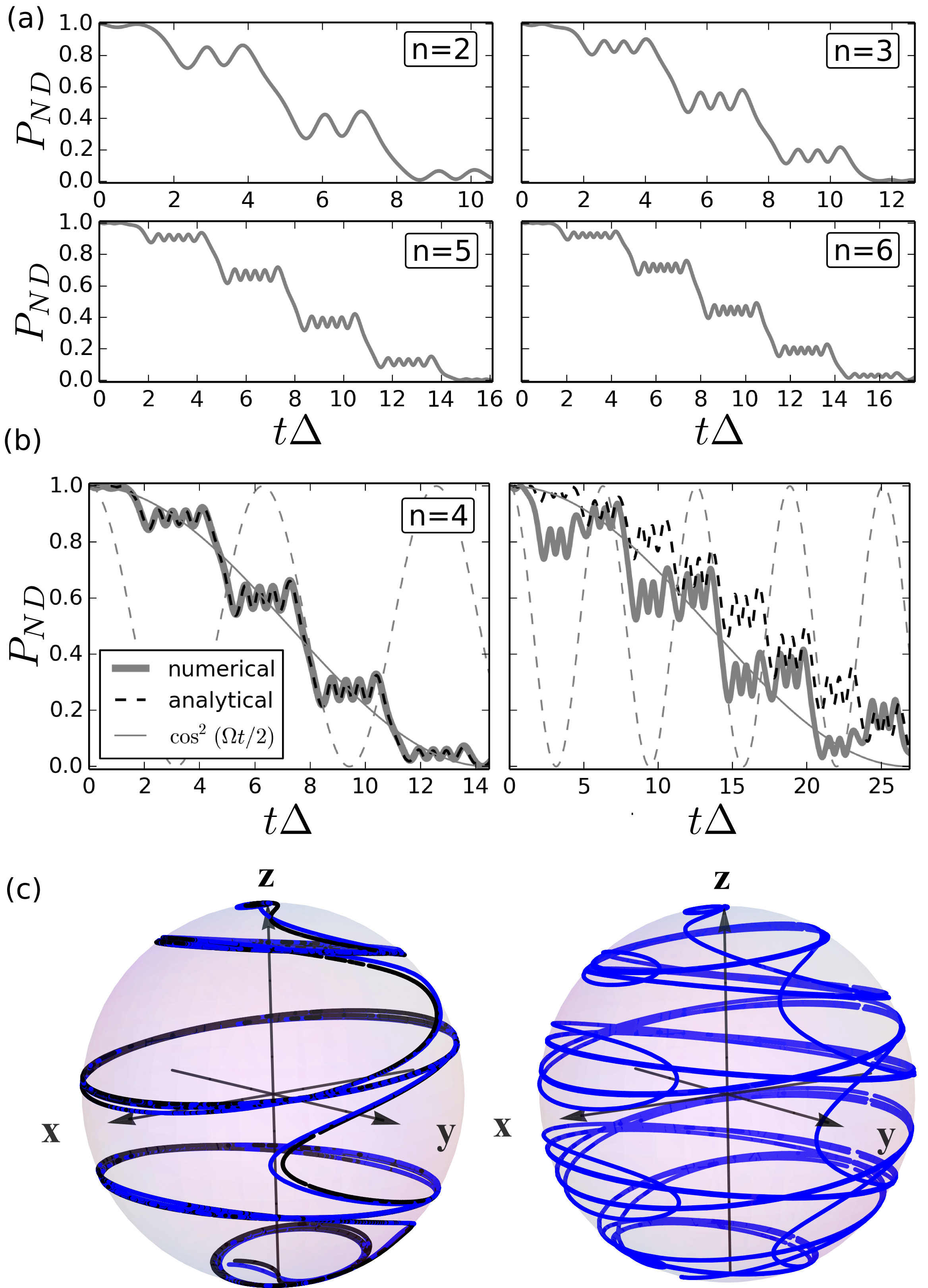
Figure 2: (Color online) Time evolution of the non decay probability for the system starting in state $\left|0\right>$, in the resonant ($\omega=\Delta$) regime. (a) Amplitudes corresponding to peaks $n=2,3,5,6$. (b) Left: Amplitude corresponding to $n=4$. Right: $A=4.5\omega$, between $n=2$ and $n=3$. Thick lines show the results given by numerical simulations, while the black dashed curve is given by the analytical solution (see text for details). For comparison, we show the solution predicted in the high frequency regime (solid light gray line), and a cosine function with the frequency of the driving field, $\omega$ (dashed light gray line). (c) Time evolution of the complete state of the system, depicted in Bloch sphere, for the cases shown in (b). The analytical solution is not shown for the case $A=4.5\omega$, for clarity.

III Maximum population transfer: Bloch sphere model and analytical solution

The singular behavior shown by the dynamics at the extrema of the quasienergy spectrum admits a (deeper) analytical explanation. Hamiltonian $H_{2}$ in eq. (2) can be regarded as equivalent to the interaction of a spin-$1/2$ particle with a unit intensity magnetic field $\vec{B(t)}$ rotating periodically but non-uniformly in the $x-y$ plane, such that the instantaneous Larmor frequency is $\Delta$. The components of this field can be expanded in Fourier series

$$B_{x}(t) \equiv \mathrm{cos}\left(\gamma_{z}\right)=J_{0}\left(\nu\right)+2\sum_{n=1}^{\infty}J_{2n}\left(\nu\right)\mathrm{cos}\left(2n\omega t\right)$$ (5)

$$B_{y}(t) \equiv \mathrm{sin}\left(\gamma_{z}\right)=2\sum_{n=1}^{\infty}J_{2n-1}\left(\nu\right)\mathrm{sin}\left[(2n-1)\omega t\right],$$ (6)

where $\nu=2A/\omega$. If considered separately, the time integrals of both components give the accumulated phase throughout the evolution. As shown in Fig. 3, the contribution $\gamma_{x}(t)\equiv\int_{0}^{t}B_{x}(s)ds$ shows the ladder structure found previously, as the result of integrating a constant term added to an oscillating series. On the other hand, integrating $B_{y}(t)$ shows that the leading term vanishes when $J_{1}(2A/\omega)=0$, this resulting in a small phase contribution of the whole series. Also notice that, because of the relation $J^{\prime}_{0}(x)=-J_{1}(x)$, the zeros of $J_{1}$ match the extrema of $J_{0}$, also giving the position of the spectrum peaks mentioned above, as long as approximation (4) holds. In this situation, $U_{2}(t)$ is well approximated by $U_{2}(t)=\mathrm{exp}\left[-\frac{i}{2}\gamma_{x}(t)\sigma_{x}\right]=\mathrm{exp}\left\{-\frac{i}{2}\left[\Delta^{\prime}t+\delta(t)\right]\sigma_{x}\right\}$ with

$$\delta(t)=\frac{\Delta}{\omega}\sum_{n}\frac{J_{2n}(2A/\omega)}{n}\>\mathrm{sin}\left(2n\omega t\right),$$ (7)

which is $T$-periodic and can be seen to vanish in the limit $\Delta/\omega\rightarrow 0$, as expected.

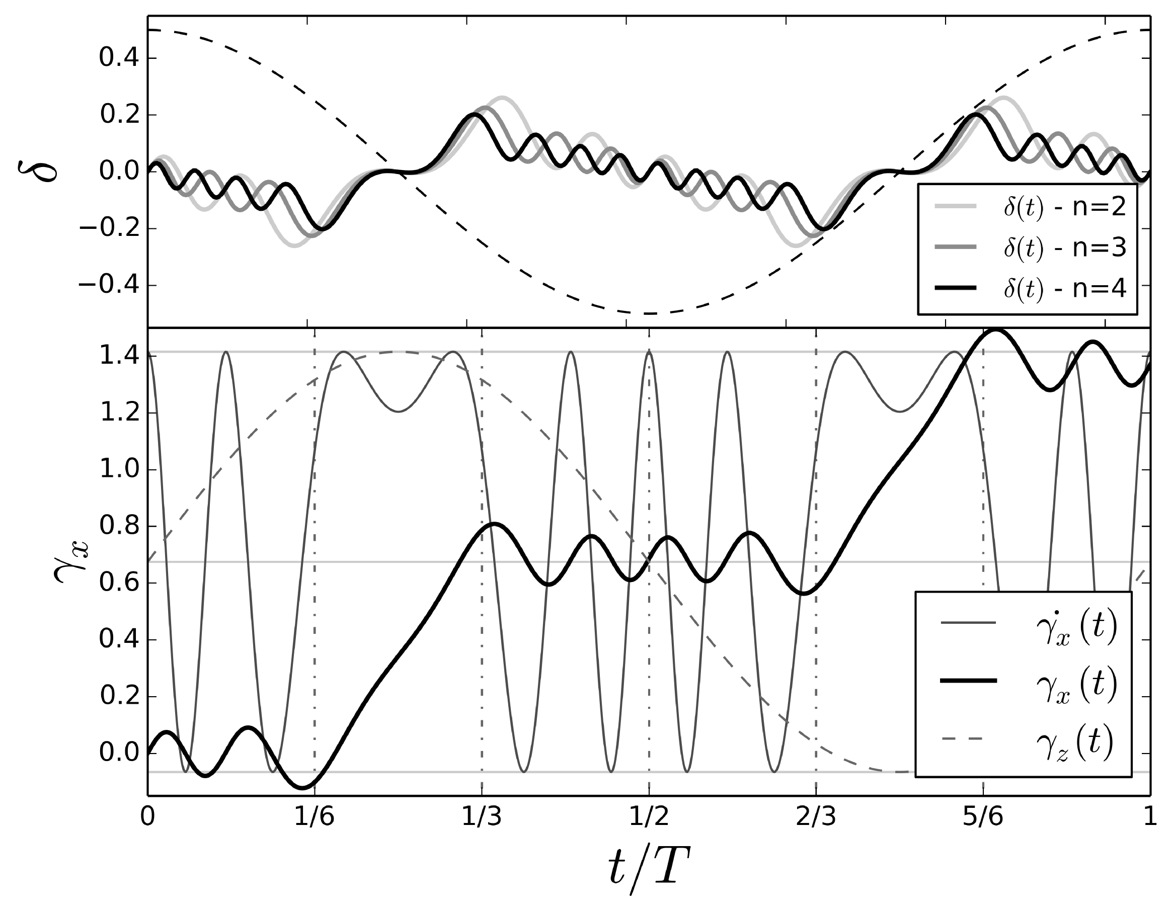
Figure 3: Top: Plots of function $\delta(t)$ defined by Eq. (7), over one period of the driving field, for different values of amplitude corresponding to $n=2,3,4$. In dashed lines a cosine function with the frequency of the driving field $\omega$ is shown. Bottom: Plot of the time-dependent phases $\gamma_{x}(t)$ and $\gamma_{z}(t)$ which appear in the analytical solution $U(t)$ proposed for the evolution operator. Also shown is $B_{x}(t)=\dot{\gamma_{x}}(t)$. Note that the left axis labels correspond only to $\gamma_{x}(t)$, the remaining functions being properly normalized for comparision.

Plots of $\delta(t)$ for different values of $n$ are displayed in Fig. 3. This model approximates very well the population dynamics when the field parameters are set at the extrema of the quasienergy spectrum. A representative example is shown in Fig. 2. In this case the full evolution operator becomes

$$U=U_{1}U_{2}=\mathrm{exp}\left[-i\gamma_{z}(t)\sigma_{z}/2\right]\mathrm{exp}\left[-i\gamma_{x}(t)\sigma_{x}/2\right],$$ (8)

and the particular time-dependence of $\gamma_{x}$ and $\gamma_{z}$ over one period of the driving field (see Fig. 3) allows to rationalize the resulting dynamics, as follows. Let us consider a partition of the driving period in six equal intervals, each one of length $T/6$. Then $\gamma_{x}(t)$ and $\gamma_{z}(t)$ can be approximated as a sequence of linear and constant pieces, both showing opposite behaviors during the interval. That is, from $t=T/6$ to $t=2T/6$, $\gamma_{z}$ is almost constant and $\gamma_{x}$ increases with a positive slope; the resulting $U(t)$ being then well approximated by a $x$-rotation in Bloch sphere. From $t=2T/6$ to $t=3T/6$ (and also in the following interval) $\gamma_{x}$ shows low-amplitude oscillations around a steady value, while $\gamma_{z}$ decreases in time almost linearly; $U(t)$ will then produce rapid rotations around the $z$-axis rendering nearly constant populations. Similarly, we can continue with the rest of the intervals in the period. Finally, note that this discussion also accounts for the phenomenon of optimal population transfer at these points, shown in Fig. 1. Using this model, a simple calculation gives $P_{ND}(T_{F})=\mathrm{sin}^{2}\left(\delta(T_{F})/2\right)$, which is numerically seen never exceeding $10^{-2}$.

IV An example: control of isomerization reactions

Let us discuss next the application of our results in a molecular control problem bib:int_prac . For this purpose, we consider the LiNC/LiCN molecular system that has been extensively studied in connection with the theoretical issue of quantum chaos bib:LiCN , and also in the simulation of the LiNC$\rightleftharpoons$LiCN isomerization reaction bib:Hase in solution, where it was proven to provide the first unambiguous example of the elusive Kramers turnover bib:Muller . In general, isomerization reactions have generated a lot interest from the theoretical side bib:Hase and also for their practical importance in many relevant chemical processes, specially of biological interest iso1 ; iso2 ; iso3 ; iso4 . For example, the control of the HCN isomerization was thoroughly studied in Refs. control_HCN_1 ; control_HCN_2 ; control_HCN_3 , and the importance of intermediate states with configurations far from the usual ones discussed.

IV.1 The LiNC/LiCN molecular system

The LiNC/LiCN isomerizing system presents two stable isomers at the linear configurations: Li–N–C and Li–C–N, which are separated by a relatively modest energy barrier of only 0.0157376 a.u. The C and N atoms are strongly bounded by a triple covalent bond, while the Li is attached to the CN moiety by mostly ionic forces, due to the large charge separation existing between them. For these reasons, the CN vibrational mode effectively decouples from the other degrees of freedom of the molecule, and it can be considered frozen at its equilibrium value, $r_{e}=2.186$. On the other hand, the relative position of Li with respect to the center of mass of the CN is much more flexible. In particular the bending along the angular coordinate is very floppy, and the corresponding vibration performs very large amplitude motions even at moderate values of the excitation energy. Accordingly, the vibrations of the whole system can be adequately described by the following 2 degrees of freedom. Using scattering or Jacobi coordinates $(R,r,\theta)$, where $R$ is the distance from the Li atom to the center of mass of the CN fragment, $r$ the C–N distance, and $\theta$ the angle formed by these two vectors, the corresponding classical ($J=0$) Hamiltonian is given by

$$H=\frac{P_{R}^{2}}{2\mu_{\mathrm{Li-CN}}}+\frac{1}{2}\left(\frac{1}{\mu_{\mathrm{Li-CN}}R^{2}}+\frac{1}{\mu_{\mathrm{CN}}r_{e}^{2}}\right)P_{\theta}^{2}+V(R,\theta),$$ (9)

where $P_{R}$ and $P_{\theta}$ are the associate conjugate momenta, and the corresponding reduced masses are given by $\mu_{\mathrm{Li-CN}}=m_{\mathrm{Li}}m_{\mathrm{CN}}/(m_{\mathrm{Li}}+m_{\mathrm{CN}})=10072$ and $\mu_{\mathrm{CN}}=m_{\mathrm{C}}m_{\mathrm{N}}/m_{\mathrm{CN}}=11780$.

Note that we assume that the isomerization process is fast compared with the rotation of the molecule. The potential interaction, $V(R,\theta)$, is given by a 10–terms expansion in Legendre polynomials,

$$V(R,\theta)=\sum_{\lambda=0}^{9}v_{\lambda}(R)P_{\lambda}(\cos\theta),$$ (10)

where the coefficients, $v_{\lambda}(R)$, are combinations of long and short–term interactions whose actual expressions have been taken from the literature LiCN.PES . This potential, which is shown in Fig. 4 (a) as a contour plot, has a global minimum at $(R,\theta)=(4.349,\pi)$, a relative minimum at $(R,\theta)=(4.795,0)$, and a saddle point at $(R,\theta)=(4.221,0.292\pi)$. The two minima correspond to the stable isomers at the linear configurations, LiNC and LiCN, respectively. The LiNC configuration, $\theta=\pi$, is more stable than that for LiCN, $\theta=0$. The minimum energy path connecting the two isomers has also been plotted superimposed in the figure with dashed line.

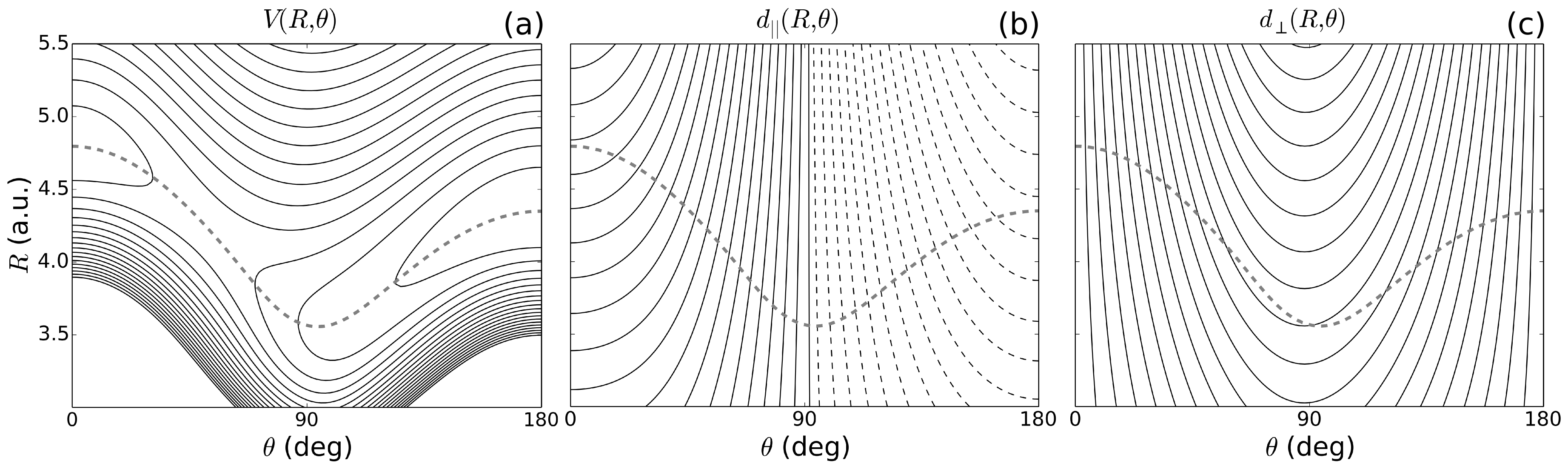
Figure 4: Contour plot representation in the configuration space $(R,\theta)$ for the following functions of the LiNC/LiCN isomerizing system: (a) Potential energy surface $V(R,\theta)$ (contours every 1000 cm^-1 starting from zero). (b) Dipole moment component parallel to the N–C bond (contours every 0.25 a.u. starting from zero, dashed lines correspond to negative values). (c) Same as (b) for the perpendicular component. The minimum energy path connecting the isomer wells has been superimposed as a grey thick dashed line in the three plots.

The LiCN molecule is a polar molecule, i.e., it has a permanent dipole moment, so that in the presence of an electric field, $\vec{{\cal E}}$, an additional potential energy term appears, this leading to the following effective Hamiltonian function

$$H=H_{\mathrm{LiCN}}-\vec{d}(R,\theta)\cdot\vec{{\cal E}},$$ (11)

where $\vec{d}(R,\theta)$ is the dipole moment of the LiNC/LiCN molecular system. For the dipole moment, we have taken from the literature the ab initio calculations fitted to an analytic expansion in associated Legendre functions of Brocks et al. bib:brocks . The corresponding components parallel and perpendicular to the N–C bond are shown in Fig. 4 (b) and (c), respectively.

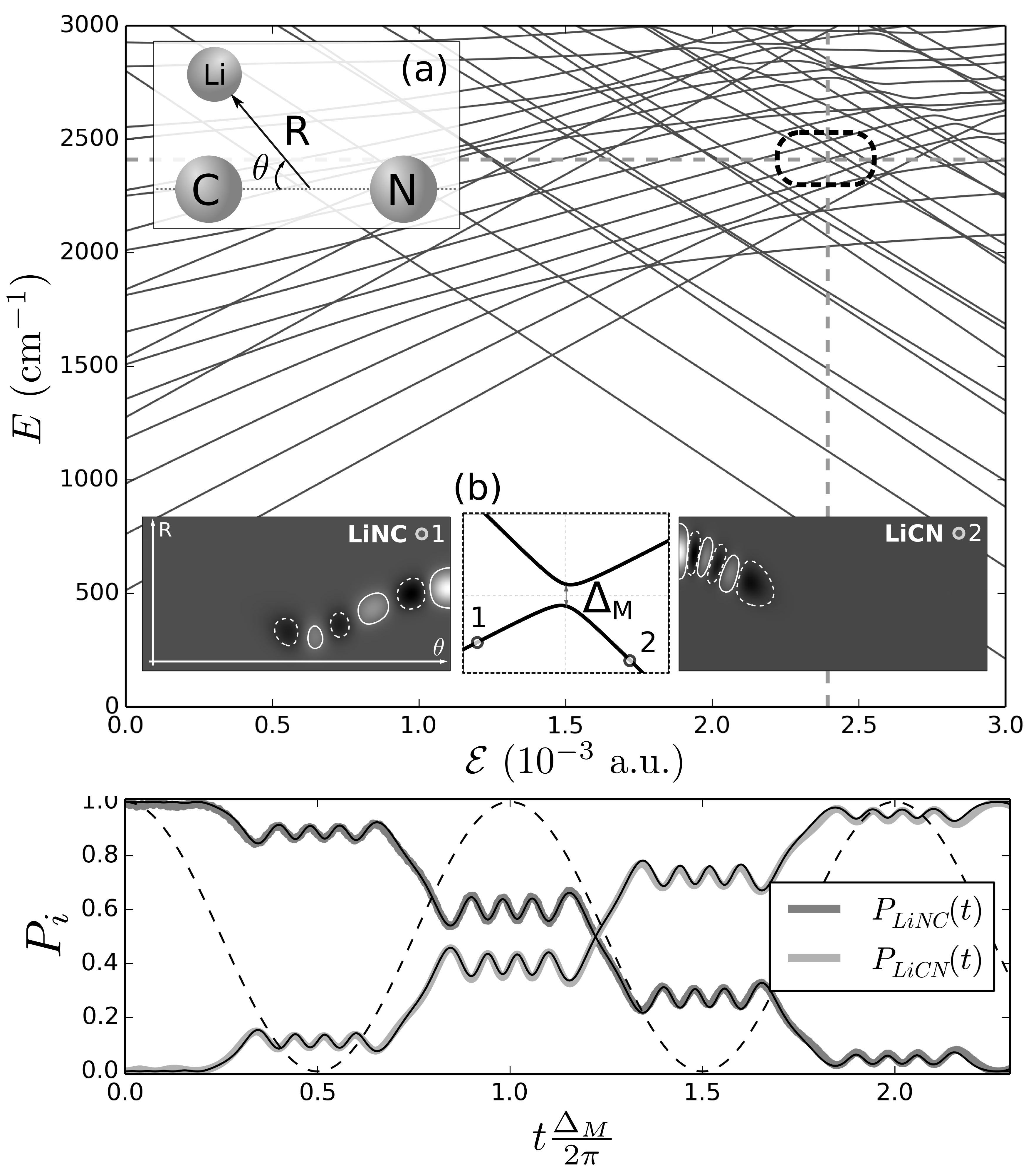
Figure 5: Top: (main) energy spectrum of the LiNC/LiCN molecular system as a function of the electric field intensity $\cal{E}$. (a) Schematic diagram of the LiCN molecule, including the set of coordinates $(R,\theta)$ used. (b) Enlarged view of the squared zone of the spectrum, showing the AC considered in the control strategy. At both sides, density plots of the wavefunctions far from the AC, which represent excited isomerized states. The axis ranges are $0<\theta<180^{\circ}$ and $3<R<5.5$ a.u. Bottom: numerically simulated population evolution, starting in state $\left|1\right>$ and setting $\omega=\Delta_{M}$ and $A=(1.23\times 10^{-2})\Delta$. Full black lines show the result predicted by the two-level analytical solution (8) applied to this system.

IV.2 Achieving isomerization via a DC+AC field

In order to design an effective control strategy, we consider the electric field to be parallel to the C$\rightarrow$N bond and compute the vibrational level spectrum as a function of the (static) electric field intensity $\cal{E}$, as previously proposed in Refs. bib:murgida ; bib:poggi . In order to do so, we used the discrete variable representation - distributed Gaussian basis (DVR-DGB) method introduced in Ref. bib:bacic . Results are shown in Fig. 5. As a rule of thumb, positive-slope energy lines correspond to LiNC states (that is, those localized in the $\theta=180^{\circ}$ well), and the negative-slope lines to LiCN states ($\theta\sim 0$). Further details on the structure of this spectrum can be found on Refs. Arranz1 ; Arranz2 .

A careful analysis of the spectrum shows that most ACs in the low-energy region are very narrow and thus correspond to interactions too weak to be useful in the control process. However, there is an AC centered at $\mathcal{E}=\mathcal{E}_{\rm{dc}}\equiv 2.39\times 10^{-3}$ a.u., with a spectral gap of $\Delta_{M}=0.15$ cm^-1 which seems suitable for our purposes. Indeed, far for from the AC, the involved eigenstates, termed $\left|\mathrm{LiNC}\right>$ and $\left|\mathrm{LiCN}\right>$, show localization in opposite wells (see Fig. 5-b) as needed in the control process. We thus analyze the use of an electric field of the form: $\mathcal{E}(t)=\mathcal{E}_{\mathrm{dc}}+A\mathrm{cos}\left(\omega t\right)$.

The main feature to be emphasized here is that the results drawn from usual high driving frequency regime could not be applied in this case. This is because the quasienergy spectrum is a function of the ratio $A/\omega$, which means that high values of $\omega$ would then imply the use of large amplitudes. Note that, in such case, the control parameter (i.e., $\mathcal{E}$ in our case) would reach zones of the energy spectrum where more levels are involved in an effective interaction. This would invalidate the two-level approximation in a many level system showing multiple ACs, like ours. This can be clearly seen in Fig. 6, where we show the quasienergy spectrum of our molecular system as a function of $A^{\prime}/{\omega}$ bib:aclaracion , for different values of driving frequency $\omega$. Note that only the region of the spectrum corresponding to the marked AC in the Fig. 4 (b) of the main text is displayed here. As can be seen, the ribbon structure typical of the kind of system considered in this work becomes clearly distorted as the frequency increases. Therefore, we propose to work in the intermediate frequency regime discussed before, so that the main results of the previous sections become relevant for this problem. Actually, setting $\omega$ equal to $\Delta_{M}$ make expressions (1) to (8) straightforwardly applicable. As an illustration, we show in the bottom panel of Fig. 5 the evolution obtained starting from state $\left|LiNC\right>$ bib:otromet for $A=(1.23\times 10^{-2})\Delta$ (corresponding to $n=4$). In terms of control efficiency and suitability, we point out that the total control time is approximately $2.3\times 2\pi/\Delta_{M}\simeq 0.51$ ps, which is well below the $400$ ps reported in Ref. bib:murgida . Nevertheless, it should be noted that this protocol would require fine tuning of the control parameters, similarly to more elemental strategies (such as applying a single pi-pulse. We remark that the results predicted by the analytical model proposed in Sec. IV are in full agreement with the numerical results, as can be seen in Fig. 5.

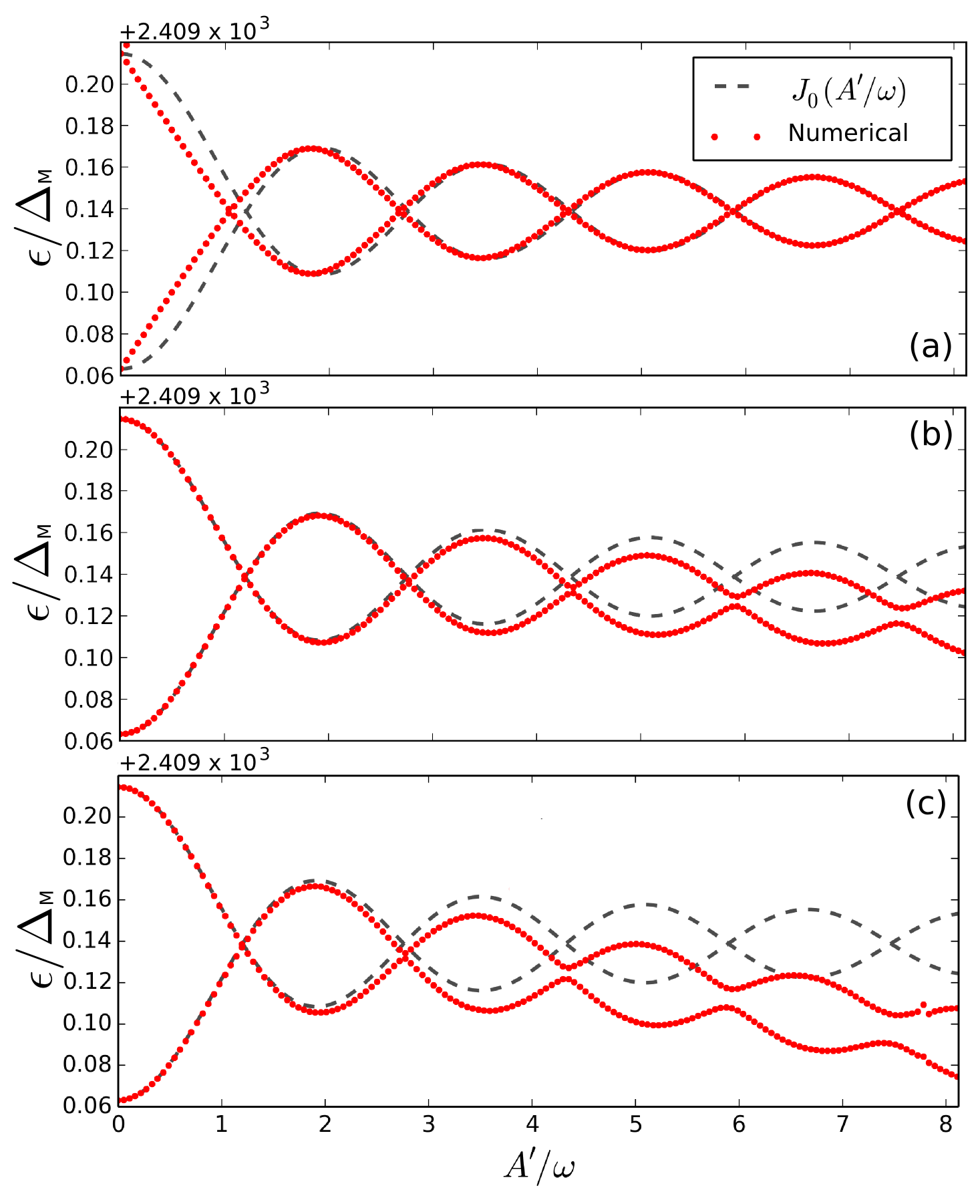
Figure 6: (Color online) Quasienergy spectrum for the LiNC/LiCN molecular system, focused in the energy range of the avoided crossing under study (see Fig. 5). The values of driving field frequency used in each case are: (a) $\omega=\Delta_{M}$, (b) $\omega=20\Delta_{M}$, (c) $\omega=30\Delta_{M}$.

V Final remarks

In summary, we have shown the existence of a set of special points in the quasienergy spectrum of a periodically-driven TLS, where the evolution of the populations takes place with maximum probability transfer. These points correspond to the maxima and minima in the typical ribbon structure exhibited by the spectrum, localized between the degeneracies predicted by the occurrence of CDT. We have also shown that for these particular combinations of the driving parameters the full evolution operator for the system can be well approximated by a very simple analytical expression, which reveals that the system evolves in a Bloch sphere following a sequence of rotations around the $x$ and $z$ axes. This behavior reflects in the appearance of a series of steps in the time evolution of the populations, whose average takes the form of a decreasing “ladder”, a behaviour which has been reported in previous works on this model bib:nori ; bib:vitanov It should be noted that these results correspond to the intermediate frequency regime ($\omega\simeq\Delta$) where the RWA does not apply. Finally, we have made use of these conclusions to study the isomerization process induced by an oscillating electric field applied to a triatomic molecule. Using this realistic model, we have shown that the regime described in this Letter is particularly relevant in many level systems showing multiple ACs, where the use of large-amplitude driving fields would make the simple two-level approximation invalid. We also believe that the results shown in this Letter could be of great interest to the vast ongoing research on driven superconducting qubits bib:valenzuela , usually modelled also by hamiltonian (1).

- (1) M. Shapiro and P. Brumer, Quantum Control of Molecular Processes (Wiley-VCH, Berlin, 2011).
- (2) H.M. Wiseman and G.J. Milburn, Quantum Measurement and Control (Cambridge University Press, Cambridge, 2009).
- (3) M.A. Nielsen and I.L. Chuang, Quantum computation and quantum information (Cambridge University Press, Cambridge, 2000).
- (4) C. Zener, Proc. R. Soc. London, Ser. A 137, 696 (1932).
- (5) S.I. Chu and D.A. Telnov, Phys. Rep. 390, 1 (2004).
- (6) S. Ashhab, J. R. Johansson, A. M. Zagoskin, and F. Nori, Phys. Rev. A 75, 063414 (2007).
- (7) Y. Wu and X. Yang, Phys. Rev. Lett. 98, 013601 (2007).
- (8) E. Barnes and S. Das Sarma, Phys. Rev. Lett. 109, 060401 (2012).
- (9) F. Grossmann, T. Dittrich, P. Jung, and P. Hänggi, Phys. Rev. Lett. 67, 516 (1991).
- (10) E. Kierig, U. Schnorrberger, A. Schietinger, J. Tomkovic, and M. K. Oberthaler, Phys. Rev. Lett. 100, 190405 (2008); A. Zenesini, H. Lignier, D. Ciampini, O. Morsch, and E. Arimondo, Phys. Rev. Lett. 102, 100403 (2009).
- (11) M. Holthaus, Phys. Rev. Lett. 69, 351 (1992); M. Holthaus and D. Hone, Phys. Rev. B 47, 6499 (1993).
- (12) Note that we set throughout the Letter.
- (13) G. Brocks, J. Tennyson, and A. van der Avoird, J. Chem. Phys. 80, 3223 (1984). Notice that there is a typo in this reference: the coefficients and for the dipole moment expansion of LiCN in Table II should be negative instead positive signed.
- (14) G. E. Murgida, D. A. Wisniacki, P. I. Tamborenea, and F. Borondo, Chem. Phys. Lett. 496, 356 (2010).
- (15) C.E. Creffield, Phys. Rev. B 67, 165301 (2003).
- (16) K. Hijii and S. Miyashita, Phys. Rev. A 81, 013403 (2010).
- (17) B.M. Garraway and N.V. Vitanov, Phys. Rev. A 55, 4418 (1997).
- (18) C. A. Arango and P. Brumer, J. Chem. Phys. 138, 071104 (2013);
- (19) F. J. Arranz, L. Seidel, C. G. Giralda, R. M. Benito, and F. Borondo, Phys. Rev. E 87, 062901 (2013); Phys. Rev. E 82, 026201 (2010); F. J. Arranz, R. M. Benito, and F. Borondo, J. Chem. Phys. 120, 6516 (2004); J. Chem. Phys. 123, 044301 (2005); F. J. Arranz, F. Borondo, and R. M. Benito, Phys. Rev. Lett. 80, 944 (1998).
- (20) T. Baer and W. H. Hase, Unimolecular Reaction Dynamics: Theory and Experiments (Oxford University Press, Oxford, 1996).
- (21) P. L. García-Müller, F. Borondo, R. Hernandez and R. M. Benito, Phys. Rev. Lett. 101, 178302 (2008); J. Chem. Phys. 137, 204301(2012).
- (22) G. Vogt, G. Krampert, P. Niklaus, P. Nuernberger, and G. Gerber, Phys. Rev. Lett. 94, 068305 (2005).
- (23) B. Dietzek, B. Brüggemann, T. Pascher, and A. Yartsev, Phys. Rev. Lett. 97, 258301 (2006).
- (24) V. I. Prokhorenk, A. M. Nagy, S. A. Waschuk, L. S. Brown, R. R. Birge, and R. J. Dwayne Miller, Science 313, 1257 (2006).
- (25) T. T. To, E. J. Heilweil, R. Duke III, K. R. Ruddick, C. E. Webster, and T. J. Burkey, J. Phys. Chem. A 113, 2666 (2009).
- (26) B. L. Lan and J. M. Bowman, J. Chem. Phys. 101, 8564 (1994).
- (27) W. Jakubetz and B. L. Lan, Chem. Phys. 217, 375 (1997).
- (28) S. P. Shah and S. A. Rice, J. Chem. Phys. 113, 15 (1999).
- (29) R. Essers, J. Tennyson, and P. E. S. Wormer, Chem. Phys. Lett. 89, 223 (1982).
- (30) P. M. Poggi, F. C. Lombardo and D. A. Wisniacki, Phys. Rev. A 87, 022315 (2013).
- (31) Z. Bacic and J.C. Light, J. Chem. Phys. 85, 4594 (1986).
- (32) F. J. Arranz, R. M. Benito, and F. Borondo, J. Chem. Phys. 123, 044301 (2005); J. Chem. Phys. 120, 6516 (2004).
- (33) F. J. Arranz, R. M. Benito, and F. Borondo, J. Chem. Phys. 107, 2395 (1997).
- (34) Note that the AC in model (1) is symmetrical; in the general case, the slopes of the diabatic branches must be taken into account. This leads to the rescaling , where is the difference of slopes between the branches (in absolute value).
- (35) Note that preparing the system in state can be done by exciting the molecule at zero field and then adiabatically tuning the field from to , as explained in Refs. bib:murgida ; bib:poggi .
- (36) M. S. Rudner, A. V. Shytov, L. S. Levitov, D. M. Berns, W. D. Oliver, S. O. Valenzuela, and T. P. Orlando, Phys. Rev. Lett. 101 190502 (2008).