Energy Driven Pattern Formation in Planar Dipole–Dipole Systems in the Presence of Weak Noise

Abstract

We study pattern formation in planar fluid systems driven by intermolecular cohesion (which manifests as a line tension) and dipole–dipole repulsion which are observed in physical systems including ferrofluids in Hele-Shaw cells and Langmuir layers. When the dipolar repulsion is sufficiently strong, domains undergo forked branching reminiscent of viscous fingering. A known difficulty with these models is that the energy associated with dipole–dipole interactions is singular at small distances. Following previous work, we demonstrate how to ameliorate this singularity and show that in the macroscopic limit only the scale of the microscopic details relative to the macroscopic extent of a system is relevant and develop an expression for the system energy that depends only on a generalized line tension, $\Lambda$, that in turn depends logarithmically on that scale. We conduct numerical studies that use energy minimization to find equilibrium states. Following the subcritical bifurcations from the circle, we find a few highly symmetric stable shapes, but nothing that resembles the observed diversity of experimental and dynamically simulated domains. The application of a weak random background to the energy landscape stabilizes a smörgåsbord of domain morphologies recovering the diversity observed experimentally. With this technique, we generate a large sample of qualitatively realistic shapes and use them to create an empirical model for extracting $\Lambda$ with high accuracy using only a shape’s perimeter and morphology .

I Introduction

A wide variety of two-dimensional systems driven by competition between strong, short-ranged attractive and long-ranged, dipole-like repulsive forces exhibit striking phenomenological similarities. This interplay leads to the formation of intricate and tree-like structures. Substantial work has been done in characterizing the physics, dynamics, and morphology of these systems Cebers (1980); Cebers and Maiorov (1980a); Cebers and Mayorov (1980); Cebers and Maiorov (1980b); Cebers and Zemitis (1983); McConnell and Moy (1988); Vanderlick and Moehwald (1990); McConnell (1990); McConnell and de Koker (1992); Langer et al. (1992); Dickstein et al. (1993); Goldstein and Jackson (1994); Jackson et al. (1994); de Koker and McConnell (1994); de Koker et al. (1995); Lubensky and Goldstein (1996); Seul and Andelman (1995); McConnell and de Koker (1996); Cebers and Drikis (1996, 1999); Mann and Primak (1999); Khattari and Fischer (2002); Elias et al. (1998); Otto (1998); Cebers and Drikis (1999); Khattari and Fischer (2002); Heinig et al. (2004); Hillier and Jackson (2007); Jackson (2008). Langmuir monolayers Vanderlick and Moehwald (1990); de Koker and McConnell (1994); Lubensky and Goldstein (1996); McConnell and de Koker (1996); Mann and Primak (1999); Khattari and Fischer (2002) and ferrofluid confined to a Hele-Shaw cell Cebers (1980); Cebers and Maiorov (1980a); Cebers and Mayorov (1980); Cebers and Maiorov (1980b); Cebers and Zemitis (1983); Vanderlick and Moehwald (1990); Langer et al. (1992); Dickstein et al. (1993); Jackson et al. (1994); Goldstein and Jackson (1994); de Koker and McConnell (1994); Lubensky and Goldstein (1996); McConnell and de Koker (1996); Cebers and Drikis (1996); Elias et al. (1998); Cebers and Drikis (1999); Khattari and Fischer (2002); Hillier and Jackson (2007); Jackson (2008) are of particular interest, and shape formation and stability in these systems have been studied extensively in experiment (see examples in Fig. 1(a–d)).

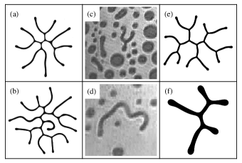
Figure 1: Examples of two-dimensional dipole-mediated systems in experiments. (a, b) Ferrofluid enclosed in a Hele-Shaw cell. Images provided by D. P. Jackson Goldstein and Jackson (1994); Dickstein et al. (1993); Langer et al. (1992). (c, d) 8–CB Langmuir films, or monolayers of polymer molecules, condensed into their fluid phase. Images provided by E. K. Mann Mann and Primak (1999). (e, f) Results of our numeric simulations.

The inherent complexity of dipole-mediated systems has also inspired numerical simulations using dynamic evolution of some particular system’s equations of motion Alexander et al. (2007); Dickstein et al. (1993); Heinig et al. (2004); Jackson et al. (1994); Lubensky and Goldstein (1996); Tucker (2008); Cebers and Drikis (1999, 1996); Cebers and Zemitis (1983); Elias et al. (1998). For example, Cebers et al. Cebers and Drikis (1999); Cebers and Maiorov (1980a) and Jackson et al. Langer et al. (1992); Dickstein et al. (1993) considered Hele-Shaw systems, providing analytic and asymptotic expressions for the energy and stability of a variety of domain structures, including circles and rectangles. McConnell et al. built an effective theoretical formalism for describing the energy of Langmuir domains, and determined analytically the stability of circular and stripe domains to harmonic perturbations Vanderlick and Moehwald (1990); McConnell (1990); McConnell and de Koker (1992); de Koker et al. (1995). McConnell et al. were able to show that the detailed physical parameters that describe Langmuir systems can be reduced to a single parameter de Koker and McConnell (1993). Though this reduction greatly simplifies the state space of these systems, it does not appear to have been used by other researchers after McConnell. The energy formalism that we will introduce here, though different from the one used by McConnell et al., proceeds along nearly identical lines to reduce the parameter space to one dimension. We use this energy formalism numerically to realize static equilibrium states via energy extremization. These methods can resolve subcritical branches for harmonic bifurcations associated with the hysteresis discovered by Cebers et al. Cebers and Zemitis (1983) and later studied by Jackson and his collaborators Hillier and Jackson (2007); Jackson (2008). In the absence of noise, we discovered stable domains are characterized by a few, highly symmetric morphologies. We argue that the rich qualitative structure seen in dynamic studies and experiment is due to the presence of random imperfections modelled as variations in the energy landscape, and show that a simple empirical rule exists for accurately determining the state parameter of dipole-mediated systems.

II Analysis

Consider a compact region $\Omega\subset\mathbb{R}^{2}$ which describes the spatial extent of a dipole-mediated domain. The energy of such a domain is given by McConnell (1990); Kent-Dobias (2014)

$$E=\alpha A+\lambda\ell+\frac{\mu^{2}}{2}\iint\limits_{\Omega}\iint\limits_{\Omega}\frac{g(\left\|\boldsymbol{\mathbf{r}}-\boldsymbol{\mathbf{r}}^{\prime}\right\|)}{\left\|\boldsymbol{\mathbf{r}}-\boldsymbol{\mathbf{r}}^{\prime}\right\|^{3}}\,d{A^{\prime}}\,dA+\iint\limits_{\Omega}V(\boldsymbol{\mathbf{r}})\,dA.$$ (1)

The first two terms are proportional to the area $A$ and the perimeter $\ell$ of $\Omega$ respectively, where $\lambda$ is the line tension. Since we only consider domains constrained to have constant area, the first term is irrelevant to system behavior and will henceforth be neglected. The third term is the energy due to the dipole–dipole interaction, a continuum approximation of mutually interacting dipole pairs. The fourth term is the energy due to an arbitrary static external potential. The constant $\mu$ is an effective dipole density, and the function $g(r)$ is the pair correlation function for the system, which gives the probability distribution that a dipole is displaced from another by $r$. In disordered systems, like the ones we consider, $g$ must be isotropic (and therefore radially symmetric), have $g(0)=0$ (as particles cannot exist atop each other), and $g(r)$ must be well approximated by $1$ if $r>\Delta$ for some interparticle length scale $\Delta$ Hansen and McDonald (1990). In order for (1) to converge, $g(r)$ must vanish at least as quickly as $r^{2}$ as $r$ tends to zero. For different physical systems $g(r)$ can take on a variety of forms, all of which are highly dependent on the microscopic details of the particular system. As we will see presently, the particular form of $g(r)$ is unimportant to the behavior of the domain when the microscopic parameter $\Delta$ is much smaller than the characteristic length scale of that domain, e.g., $\ell$.

Using Green’s theorem, we may convert (1) to a line integral over the domain’s boundary $\partial\Omega$ in an analogous fashion to that done by McConnell et al. McConnell and Moy (1988); McConnell and de Koker (1992). In this case, we have for the energy

$$E=\lambda\ell-\frac{\mu^{2}}{2}\oint\limits_{\partial\Omega}\oint\limits_{\partial\Omega}\Phi(\left\|\boldsymbol{\mathbf{r}}-\boldsymbol{\mathbf{r}}^{\prime}\right\|)(\hat{\boldsymbol{\mathbf{n}}}\cdot\hat{\boldsymbol{\mathbf{n}}}^{\prime})\,d{s^{\prime}}\,ds+\oint\limits_{\partial\Omega}\boldsymbol{\mathbf{\Psi}}(\boldsymbol{\mathbf{r}})\cdot\hat{\boldsymbol{\mathbf{n}}}\,ds.$$ (2)

Here, $\hat{\boldsymbol{\mathbf{n}}}$ is the unit normal to the parameterization $\boldsymbol{\mathbf{s}}$, $\Phi(r)$ is such that $\boldsymbol{\mathbf{\nabla}}^{2}\Phi(r)=g(r)r^{-3}$, and $\boldsymbol{\mathbf{\Psi}}(\boldsymbol{\mathbf{r}})$ is such that $\boldsymbol{\mathbf{\nabla}}\cdot\boldsymbol{\mathbf{\Psi}}=V$. We find via direct integration of the Laplacian that

$$\Phi(r) =\int_{r}^{\infty}\frac{1}{r^{\prime}}\int_{r^{\prime}}^{\infty}r^{\prime\prime}\left[\frac{g(r^{\prime\prime})}{{r^{\prime\prime}}^{3}}\right]\,d{r^{\prime\prime}}\,d{r^{\prime}}$$ (3)

$$=\frac{g(r)}{r}+\int_{r}^{\infty}\left[\frac{g^{\prime}(r^{\prime})}{r^{\prime}}+\frac{1}{r^{\prime}}\int_{r^{\prime}}^{\infty}\frac{g^{\prime}(r^{\prime\prime})}{r^{\prime\prime}}\,d{r^{\prime\prime}}\right]\,d{r^{\prime}},$$ (4)

where we have integrated by parts twice to reach the final expression. We note that $\Phi(r)$ may have a logarithmic singularity at $r=0$ which is harmless as it is integrable. We would like to simplify this expression by considering the limit of small $\Delta$. Let the double integration in (2) be represented by

$$I\equiv\frac{1}{2}\oint\limits_{\partial\Omega}\oint\limits_{\partial\Omega}\Phi(\left\|\boldsymbol{\mathbf{r}}-\boldsymbol{\mathbf{r}}^{\prime}\right\|)(\hat{\boldsymbol{\mathbf{n}}}\cdot\hat{\boldsymbol{\mathbf{n}}}^{\prime})\,d{s^{\prime}}\,ds.$$ (5)

We may now explicitly parameterize the line integral by arc length, yielding

$$I=\frac{1}{2}\int_{0}^{\ell}\int_{0}^{\ell}\Phi(\left\|\boldsymbol{\mathbf{r}}(s)-\boldsymbol{\mathbf{r}}(s^{\prime})\right\|)[\hat{\boldsymbol{\mathbf{n}}}(s)\cdot\hat{\boldsymbol{\mathbf{n}}}(s^{\prime})]\,ds^{\prime}\,ds.$$ (6)

Defining $\sigma\equiv s^{\prime}-s$, we now reparameterize the integral to the form

$$I=\frac{1}{2}\int_{0}^{\ell}\int_{-\frac{\ell}{2}}^{\frac{\ell}{2}}\Phi(\left\|\boldsymbol{\mathbf{r}}(s)-\boldsymbol{\mathbf{r}}(s+\sigma)\right\|)[\hat{\boldsymbol{\mathbf{n}}}(s)\cdot\hat{\boldsymbol{\mathbf{n}}}(s+\sigma)]\,d\sigma\,ds.$$ (7)

Consider some function $j(r,\Delta)$ with the following two properties:

$$\lim_{\Delta\to 0}j(r,\Delta)=\frac{1}{r}\quad\text{and}\quad J(\Delta)\equiv\frac{1}{2}\int_{-\frac{\ell}{2}}^{\frac{\ell}{2}}j(|\sigma|,\Delta)\,d\sigma<\infty.$$ (8)

Adding and subtracting the same quantity involving $j(r,\Delta)$ from (7) yields

$$I=\frac{1}{2}\int_{0}^{\ell}\int_{-\frac{\ell}{2}}^{\frac{\ell}{2}}\left\{\Phi(\left\|\boldsymbol{\mathbf{r}}(s)-\boldsymbol{\mathbf{r}}(s+\sigma)\right\|)[\hat{\boldsymbol{\mathbf{n}}}(s)\cdot\hat{\boldsymbol{\mathbf{n}}}(s+\sigma)]-j(|\sigma|,\Delta)\right\}\,d\sigma\,ds+J(\Delta)\ell.$$ (9)

Now take the limit as $\Delta\to 0$ in the integrand of (9). The function $j(r,\Delta)$ behaves as described in (8). Since, as $\Delta\to 0$, $g(r)$ tends to unity for all $r\in(0,\infty)$, it follows that $g^{\prime}(r)\simeq 0$ in this range as well, and (4) yields

$$\lim_{\Delta\to 0}\Phi(r)=\frac{1}{r}.$$ (10)

Carrying this limit through within the integral, we find

$$I\simeq\frac{1}{2}\int_{0}^{\ell}\int_{-\frac{\ell}{2}}^{\frac{\ell}{2}}\left[\frac{\hat{\boldsymbol{\mathbf{n}}}(s)\cdot\hat{\boldsymbol{\mathbf{n}}}(s+\sigma)}{\left\|\boldsymbol{\mathbf{r}}(s)-\boldsymbol{\mathbf{r}}(s+\sigma)\right\|}-\frac{1}{|\sigma|}\right]\,d\sigma\,ds+J(\Delta)\ell.$$ (11)

This integral, which without the addition of $j(r,\Delta)$ would be singular, now converges. This can be seen by examining the behavior of the integrand as $\sigma\to 0$, or

$$\frac{\hat{\boldsymbol{\mathbf{n}}}(s)\cdot\hat{\boldsymbol{\mathbf{n}}}(s+\sigma)}{\left\|\boldsymbol{\mathbf{r}}(s)-\boldsymbol{\mathbf{r}}(s+\sigma)\right\|}-\frac{1}{|\sigma|}=\frac{1+\mathcal{O}(\sigma^{2})}{|\sigma|+\mathcal{O}(\sigma^{3})}-\frac{1}{|\sigma|}=\mathcal{O}(\sigma^{2}).$$ (12)

We have been able to completely remove the dependence on $g(r)$ from the integration. This may seem worrisome, since $g(r)$ implicitly contained information about the microscopic parameters of the system, like the length scale $\Delta$. This parameter still enters the energy, but now through the function $J(\Delta)$, which we have yet to choose. If we pick $j(r,\Delta)=[\Theta(r-\Delta/2)+\Theta(-r-\Delta/2)]/r$, where $\Theta$ is the Heaviside function, it follows immediately from (8) that $J(\Delta)=\log\frac{\ell}{\Delta}$, and we have

$$I=\frac{1}{2}\int_{0}^{\ell}\int_{-\frac{\ell}{2}}^{\frac{\ell}{2}}\left[\frac{\hat{\boldsymbol{\mathbf{n}}}(s)\cdot\hat{\boldsymbol{\mathbf{n}}}(s+\sigma)}{\left\|\boldsymbol{\mathbf{r}}(s)-\boldsymbol{\mathbf{r}}(s+\sigma)\right\|}-\frac{1}{|\sigma|}\right]+\ell\log\frac{\ell}{\Delta}.$$ (13)

This choice of $j(r,\Delta)$ is motivated mostly by its simplicity. Many other options are available, though for consistency with the small-$\Delta$ approximation one usually must then expand $J(\Delta)$ about $\frac{\Delta}{\ell}=0$ and use the highest order term. In any such case, given the asymptotic behavior of $j(r,\Delta)$ as defined above, the highest order term will be proportional to $\log\frac{\ell}{\Delta}$, and the particular choice of $j$ will only modify the proportionality constant. The error due to taking this macroscopic limit in (11) goes as $\Delta^{3}$ Kent-Dobias (2014).

We are now able to write a more explicit form of the energy function (2),

$$E=\lambda\ell-\frac{\mu^{2}}{2}\oint\limits_{\partial\Omega}\int_{-\frac{\ell}{2}}^{\frac{\ell}{2}}\left[\frac{\hat{\boldsymbol{\mathbf{n}}}(s)\cdot\hat{\boldsymbol{\mathbf{n}}}(s+\sigma)}{\left\|\boldsymbol{\mathbf{r}}(s)-\boldsymbol{\mathbf{r}}(s+\sigma)\right\|}-\frac{1}{|\sigma|}\right]\,d\sigma\,ds-\mu^{2}\ell\log\frac{\ell}{\Delta}+\oint\limits_{\partial\Omega}\boldsymbol{\mathbf{\Psi}}(\boldsymbol{\mathbf{r}})\cdot\hat{\boldsymbol{\mathbf{n}}}\,ds.$$ (14)

To fully describe a system we are modelling, one must also enforce that the area of the domain is constant, or

$$A=\iint\limits_{\Omega}dA=\frac{1}{2}\oint\limits_{\partial\Omega}\hat{\boldsymbol{\mathbf{z}}}\cdot\bigg{(}\boldsymbol{\mathbf{r}}\times\frac{\partial\boldsymbol{\mathbf{r}}}{\partial s}\bigg{)}\;ds.$$ (15)

Note that, in the absence of the last term describing an auxiliary field, (14) is precisely what was found by McConnell et al. de Koker and McConnell (1993). However, in that study, the expression is derived for a particular $g(r)$, while we have now shown that any typical $g(r)$ will lead to a system described by the same energy. It will be convenient to non-dimensionalize this system for ease of analysis and numerics. First, define $R\equiv\sqrt{A/\pi}$, the characteristic radius of the domain. Then define

$$F\equiv\frac{E}{\mu^{2}R}, L\equiv\frac{\ell}{R}, \Lambda\equiv\frac{\lambda}{\mu^{2}}-\log\frac{R}{\Delta}, \boldsymbol{\mathbf{\rho}}\equiv\frac{\boldsymbol{\mathbf{r}}}{R}, \boldsymbol{\mathbf{\Pi}}\equiv\frac{\boldsymbol{\mathbf{\Psi}}}{\mu^{2}R}.$$ (16)

Upon substitution of these quantities into (14) and simplification, the nondimensional energy is

$$F=\Lambda L-\frac{1}{2}\oint\limits_{\partial\Omega}\int_{-\frac{L}{2}}^{\frac{L}{2}}\left[\frac{\hat{\boldsymbol{\mathbf{n}}}(s)\cdot\hat{\boldsymbol{\mathbf{n}}}(s+\sigma)}{\left\|\boldsymbol{\mathbf{\rho}}(s)-\boldsymbol{\mathbf{\rho}}(s+\sigma)\right\|}-\frac{1}{|\sigma|}\right]\,d\sigma\,ds-L\log L+\oint\limits_{\partial\Omega}\boldsymbol{\mathbf{\Pi}}(s)\cdot\hat{\boldsymbol{\mathbf{n}}}(s)\,ds.$$ (17)

When nondimensionalized, the area constraint (15) becomes

$$\pi=\frac{1}{2}\oint\limits_{\partial\Omega}\hat{\boldsymbol{\mathbf{z}}}\cdot\bigg{(}\boldsymbol{\mathbf{\rho}}\times\frac{\partial\boldsymbol{\mathbf{\rho}}}{\partial s}\bigg{)}\;ds.$$ (18)

These expressions only depend on a single parameter, $\Lambda$, and on the shape of the domain $\Omega$. The parameter $\Lambda$ can be interpreted physically as as an effective line tension, normalized by the dipole density $\mu^{2}$ and shifted by the log of the ratio of the microscopic and macroscopic length scales of the system. An interesting but perhaps unintuitive feature of this is that the instabilities we observe occur when $\Lambda$ is negative, a situation physically obtainable due to the shift.

In the limit of large $\Lambda$, the energy minimization problem is dominated by perimeter minimization and circular domains are the stable minimizer in this regime. The value of $\Lambda$ at which circular domains become unstable is of interest because it marks the transition from this simple regime to one characterized by more interesting structure. Setting $\boldsymbol{\mathbf{\rho}}(s)=\hat{\boldsymbol{\mathbf{x}}}\cos s+\hat{\boldsymbol{\mathbf{y}}}\sin s$, one can use (17) to determine the energy of a circular domain explicitly, yielding

$$F_{\circ}(\Lambda)=2\pi(\Lambda+2-\log 8)$$ (19)

matching the known result from McConnell et al. and equivalent to similar calculations by Cebers and his collaborators McConnell and Moy (1988); Cebers and Maiorov (1980a); Cebers and Mayorov (1980). Define $\Lambda_{n}$ as the critical value of $\Lambda$ at which a circular domain becomes unstable to $n$th order sinusoidal perturbations of the type $\delta\boldsymbol{\mathbf{\rho}}_{n}(\theta)=\epsilon\cos(n\theta)\boldsymbol{\mathbf{\rho}}(\theta)$. These critical values of $\Lambda$ are given by $\Lambda_{n}=\log 8-Z_{n}$, where the first few $Z_{n}$ are tabulated in McConnell (1990) and an explicit form is given in Goldstein and Jackson (1994); details of our calculation can be found in Kent-Dobias (2014). We use these critical instabilities to verify the accuracy of our numeric simulations.

Another important previous result is the calculation of the energy of a rectangular domain, which was computed previously by McConnell et al. McConnell and Moy (1988) and Langer et al. Langer et al. (1992). If $a$ is the aspect ratio of a rectangular domain, then the $x$ and $y$ dimensions of that domain are $d_{x}=\sqrt{a\pi}$ and $d_{y}=\sqrt{\frac{\pi}{a}}$, respectively. In the limit of large $a$, or high aspect ratio, we find

$$F_{\mathrm{rec}}=2\sqrt{\pi a}\left(\Lambda-\frac{1}{2}\log\frac{\pi}{a}\right)+\mathcal{O}(a^{-1/2}).$$ (20)

The value of the aspect ratio at which the above energy is minimized is $a(\Lambda)=\pi e^{-2(\Lambda+1)}$. This corresponds to a domain perimeter of $L_{\mathrm{rec}}(\Lambda)=2\pi e^{-\Lambda-1}$, and a rectangle energy of $F_{\mathrm{rec}}(\Lambda)=-2\pi e^{-\Lambda-1}$. Here, we find that as $\Lambda$ decreases, the aspect ratio of rectangular domains grows exponentially, and as a result so do their perimeters. We also find that the minimum energy of a rectangle increases exponentially with decreasing $\Lambda$. Because the energy of a rectangular domain decreases so quickly, it becomes lower than that of a circular domain when $F_{\mathrm{rec}}(\Lambda)=F_{\circ}(\Lambda)$. This transition happens at $\Lambda\simeq-1.374$. Comparing this with $\Lambda_{2}=-1.254$, the point at which the circle first becomes unstable, we see that the transition to lower rectangle energy may be related to the transition away from circles. Our numeric simulations will corroborate this, as rectangle-like domains do indeed dominate in this regime. Finally, it is important to note previous calculations of the stability of isolated stripes Cebers and Maiorov (1980a); Elias et al. (1998); de Koker et al. (1995). In our terms, they found that the critical width of a stripe, that is, the largest width for which an infinite stripe becomes unstable, is given by $d_{y}=e^{\Lambda+\gamma+2}$, where $\gamma$ is Euler’s constant. For an energy–minimized rectangle in the high aspect-ratio limit, its width is given by $w_{\mathrm{rec}}=d_{y}=e^{\Lambda+1}$, which is strictly less than the critical value for all values of $\Lambda$. This suggests that the stripe-like portions of branching structures observed in these systems are stable to perturbation.

Some researchers studying thin ferromagnetic layers use a different set of parameters than those used here Cebers and Maiorov (1980a); Jackson et al. (1994). For a magnetic fluid layer with thickness $h$, surface tension $\sigma$, and magnetic charge density $M$, our parameters translate as $\mu=Mh$, $\lambda=\sigma h$, and $\Delta\sim e^{-3/2}h$ in the limit of small thickness $h$. The generalized line tension $\Lambda$ is given, in terms of these parameters, as

$$\Lambda=\frac{3}{2}+\frac{\sigma}{M^{2}h}-\log\frac{R}{h}=\frac{3}{2}+\frac{2}{N_{B}}-\log\frac{R}{h}$$ (21)

where $N_{B}\equiv M^{2}h/\sigma$ is the magnetic bond number Jackson et al. (1994).

III Numerics

In order to perform numeric simulations of dipole-mediated domains, we discretized the boundary $\partial\Omega$ in the energy expression (17). Consider a set of $N$ points $\boldsymbol{\mathbf{x}}_{i}=(x_{i},y_{i})$, each equidistant to its adjacent neighbors. Adjacent points are kept equidistant to ensure that they are uniformly spread along the domain’s perimeter. This equidistance condition can be expressed by the $N$ consistency equations

$$\frac{L}{N}=\left\|\boldsymbol{\mathbf{x}}_{i+1}-\boldsymbol{\mathbf{x}}_{i}\right\|.$$ (22)

Define $\boldsymbol{\mathbf{\rho}}_{i}\equiv\frac{1}{2}(\boldsymbol{\mathbf{x}}_{i+1}+\boldsymbol{\mathbf{x}}_{i})$ and $\boldsymbol{\mathbf{t}}_{i}\equiv\frac{1}{2}(\boldsymbol{\mathbf{x}}_{i+1}-\boldsymbol{\mathbf{x}}_{i})$ to approximate the midpoint and tangent vectors of the polygonal sides. The normal vector $\boldsymbol{\mathbf{n}}_{i}$ is defined to be the outward facing vector orthogonal to $\boldsymbol{\mathbf{t}}_{i}$ and of the same length. The simplest discretization of the energy integration given this boundary discretization is

$$F=\Lambda L-\frac{1}{2}\sum_{i=1}^{N}\sum_{j=-N/2}^{\frac{N}{2}-1}\left(\frac{\hat{\boldsymbol{\mathbf{t}}}_{i+j}\cdot\hat{\boldsymbol{\mathbf{t}}}_{j}}{\left\|\boldsymbol{\mathbf{\rho}}_{i+j}-\boldsymbol{\mathbf{\rho}}_{j}\right\|}-\frac{1}{\frac{L}{N}|j|}\right)\frac{L^{2}}{N^{2}}-L\log L+\sum_{i=1}^{N}\boldsymbol{\mathbf{\Pi}}(\boldsymbol{\mathbf{x}}_{i})\cdot\hat{\boldsymbol{\mathbf{n}}}_{i}\frac{L}{N},$$ (23)

where the hats on some vectors denote that they have been normalized to unit length. Using (22), for instance, one can see that $\boldsymbol{\mathbf{t}}_{i}=L/N\;\hat{\boldsymbol{\mathbf{t}}}_{i}$. The expression above can be simplified considerably by computing the sum over the second term in the summand, yielding

$$F=\left(\Lambda+H_{\frac{N}{2}-1}+\frac{1}{N}\right)L-\frac{1}{2}\sum_{i=1}^{N}\sum_{\begin{subarray}{c}j=1\\ j\neq i\end{subarray}}^{N}\frac{\boldsymbol{\mathbf{t}}_{i}\cdot\boldsymbol{\mathbf{t}}_{j}}{\left\|\boldsymbol{\mathbf{\rho}}_{i}-\boldsymbol{\mathbf{\rho}}_{j}\right\|}-L\log L+\sum_{i=1}^{N}\boldsymbol{\mathbf{\Pi}}(\boldsymbol{\mathbf{x}}_{i})\cdot\boldsymbol{\mathbf{n}}_{i}.$$ (24)

where $H_{m}=\sum_{j=1}^{m}\frac{1}{j}$ is the $m$th harmonic number. In order to ensure that the area of a domain stays constant, the boundary points must fulfill the consistency expression

$$\pi=\frac{1}{2}\left\|\sum_{i=1}^{N}\boldsymbol{\mathbf{x}}_{i+1}\times\boldsymbol{\mathbf{x}}_{i}\right\|=\frac{1}{2}\left|\sum_{i=1}^{N}(x_{i}y_{i+1}-x_{i+1}y_{i})\right|.$$ (25)

We are now looking at a problem of constrained optimization; we use Lagrange multipliers to minimize (24) under the constraints (22) and (25). The Lagrangian for such a constrained system is given by

$$\mathcal{L}=F-\lambda_{0}\left[\pi-\frac{1}{2}\left|\sum_{i=1}^{N}(x_{i}y_{i+1}-x_{i+1}y_{i})\right|\right]-\sum_{i=1}^{N}\lambda_{i}\left[\frac{L^{2}}{N^{2}}-\left\|\boldsymbol{\mathbf{x}}_{i+1}-\boldsymbol{\mathbf{x}}_{i}\right\|^{2}\right],$$ (26)

where $\lambda_{0},\ldots,\lambda_{N}$ are the Lagrange multipliers. We minimize the energy of this discrete system to investigate stable domain configurations using a modified version of the Levenberg–Marquardt algorithm (LMA). Normally the LMA corresponds to a modified Newton’s method where a multiple of the identity matrix is added to the Hessian before solving for the step size. When this multiple is very large, the algorithm acts like gradient following, minimizing energy as opposed to Newton’s method which converges to any critical point. However, in a system containing Lagrange multipliers as variables, minimization of the energy with respect to all variables is impossible, since the multipliers can increase without bound and drive the algorithm to diverge. Therefore, we use LMA where, instead of an identity matrix, we add a block identity matrix to the Hessian, so that the Lagrangian is minimized with respect to the physical variables while respecting the constraints associated with the Lagrange multipliers. If $\boldsymbol{\mathbf{z}}=[x_{1},\ldots,x_{N},y_{1},\ldots,y_{N},\ell]$ is the vector of physical variables and $\boldsymbol{\mathbf{\lambda}}=[\lambda_{0},\ldots,\lambda_{N}]$ is that of Lagrange multipliers, the system is described by the state vector $[\boldsymbol{\mathbf{z}},\boldsymbol{\mathbf{\lambda}}]$. In our modified algorithm, a step is given by

$$\begin{bmatrix}\Delta\boldsymbol{\mathbf{z}}\\ \Delta\boldsymbol{\mathbf{\lambda}}\end{bmatrix}=\alpha\left(H_{\mathcal{L}}+\eta\begin{bmatrix}I_{2N+1}&0\\ 0&0\end{bmatrix}\right)^{-1}\boldsymbol{\mathbf{\nabla}}\mathcal{L}$$ (27)

where $H_{\mathcal{L}}$ and $\boldsymbol{\mathbf{\nabla}}\mathcal{L}$ are the Hessian and gradient of the Lagrangian at the previous state, $I_{n}$ is the $n\times n$ identity matrix, $\alpha$ is chosen using the Armijo rule Bertsekas (1999). The parameter $\eta$ is set to some initial value $\eta_{0}$, and then is decremented as the gradient of $\mathcal{L}$ dips below some pre-selected value.

In the absence of an external potential ($\boldsymbol{\mathbf{\Pi}}(r)=0$), we used continuation in $\Lambda$ to examine the domain shapes which are stable, i.e., energy minimizers. For sufficiently large $\Lambda$ the circular domain is the unambiguous global minimizer. Once $\Lambda\simeq\Lambda_{2}$, the phase space becomes far more interesting. We were able to follow the harmonic bifurcations from a circular domain onto their solution branches. The first five harmonic bifurcations can be seen in Fig. 2(a–f), and their branches as represented by the perimeter $L$ are plotted in the same figure. Notice that all harmonic bifurcations exhibit the same subcritical branching behavior. Stability is recovered for the $\Lambda_{2}$ branch, which corresponds to the circle to dogbone transition (see Fig. 3). This subcritical behavior has been observed previously by Cebers and his collaborators and is responsible for the hysteresis in dogbone formation and relaxation previously observed by Jackson and his collaborators Cebers and Zemitis (1983); Cebers and Drikis (1999); Hillier and Jackson (2007); Jackson (2008). We find that the value of $\Lambda$ at the tip of the upper branch is $\Lambda\simeq-1.227$. Numerically, the circle appears to be the global attractor above this point. Harmonic branches of fourfold and higher symmetries have been shown by Cebers et al. to decay into lower-symmetry shapes in magnetohydrodynamic simulations as a result of so-called vertex splitting instability Cebers and Drikis (1996, 1999). Our eigenvalue analysis confirms that these domains are unstable. We also found that the branch of threefold symmetry is unstable, despite the fact that it has not decayed in previous magnetohydrodynamic simulations Cebers and Zemitis (1983); Cebers and Drikis (1999). This inconsistency is due to the fact that the decay mechanism for the threefold symmetry is not vertex splitting—which is geometrically forbidden—and is instead caused by the atrophy of one or two of the arms, which (as we will discuss below) is a much weaker instability and would manifest itself on a much larger timescale than the vertex splitting in dynamic simulation. Moreover, previous simulations use different strategies for regularizing the dipole energy; it is plausible that this these changes effect the observed stability for, say, a small but finite magnetic layer thickness.

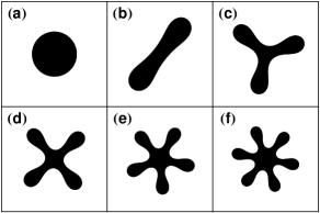
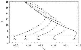
Figure 2: Bottom: The perimeters of the first five harmonic bifurcations from a circular domain. The black dots represent the theoretical bifurcation points $\Lambda_{n}$, the solid lines denote stable numeric solutions, and the dashed lines denote unstable numeric solutions. Top: A circular domain alongside those bifurcations. These shapes were taken with $\Lambda$ values of (a) $-1.2$, (b) $-1.38$, (c) $-1.52$, (d) $-1.65$, (e) $-1.69$, and (f) $-1.77$.

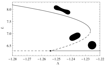
Figure 3: The subcritical bifurcation of the stripe/dogbone from the circle. The solid lines denote stable numeric solutions and the dashed lines denote unstable ones. The subcritical branch of solutions regains stability in a fold bifurcation at $\Lambda\simeq-1.227$.

If the dogbone is allowed to adiabatically evolve with decreasing $\Lambda$, it becomes long and stripe-like, very much like the rectangle we considered in the analytic section. In particular, the stripe is stable, and we suspect it is the global minimizer in the regime where the circle is no longer stable. Through bifurcation following on higher harmonic branches, we found two other stable morphologies: the forked and doubly forked domains. These are represented in Fig. 4. Notice that all three of these solutions appear like rectangles with various modifications to their ends. In fact, all three stable morphologies evolve in a similar way, becoming very long and stripe-like with large $-\Lambda$. The perimeter of these domains as a function of $\Lambda$ can be seen in Fig. 5(a). The perimeters of all three increase exponentially, and in fact almost identically to the analytic rectangle perimeter $L_{\mathrm{rec}}(\Lambda)$. The close connection between the perimeters of these stable shapes and that of $L_{\mathrm{rec}}(\Lambda)$ can be seen in Fig. 5(b), which shows the relative error between the perimeters of each stable shape and $L_{\mathrm{rec}}(\Lambda)$. As can be seen from that figure, the difference between the perimeters of these shapes and the analytic rectangle becomes less than 2% for $\Lambda\simeq-2$ and less than 1% at $\Lambda\simeq-2.5$. In fact, even the unstable higher harmonic bifurcations behave like this, approaching asymptotically the rectangle perimeter as $\Lambda$ becomes more negative.

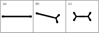
Figure 4: Representatives of (a) stripe, (b) forked, and (c) doubly forked domain morphologies at $\Lambda=-2$. These appear to be the only stable morphologies in the range of $\Lambda$ we have investigated in the absence of a random energy background.

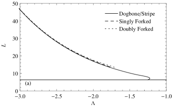
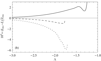
Figure 5: The asymptotic behavior of the perimeter of the three stable domain morphologies for $N=8196$. (a) The perimeter of each morphology as a function of $\Lambda$. (b) The relative error between the perimeter of each morphology and $L_{\mathrm{rec}}$, the asymptotic rectangle perimeter.

Note further that the stripe has a slightly lower perimeter than the rectangle, while the forked and doubly forked domains have progressively higher perimeters. The central bulk of the stripe is geometrically identical to the rectangle in all respects. Therefore, the curved ends of the stripe domain must be responsible for the deviation. These ends have a size proportional to the width of the stripe, which is in turn proportional to $w_{\mathrm{rec}}(\Lambda)$, the asymptotic rectangle width. The difference between the perimeters of the stripe domain and the rectangle should likewise be proportional to the size of the anomalous ends. Hence, in the limit of large negative $\Lambda$, the expressions

$$\frac{L_{\mathrm{stripe}}-L_{\mathrm{rec}}}{w_{\mathrm{rec}}} \frac{L_{\mathrm{double}}-2L_{\mathrm{forked}}-L_{\mathrm{rec}}}{w_{\mathrm{rec}}}$$ (28)

should go to the same constant $c$, loosely the energy cost per endcap. This is a nontrivial statement, since $w_{\mathrm{rec}}$ decreases exponentially as $\Lambda$ becomes more negative, so $L_{\mathrm{stripe}}-L_{\mathrm{rec}}$ will have to decrease equally exponentially in order for $c$ to converge. However, this is exactly what we see. Both expressions in (28) can be seen plotted as a function of $\Lambda$ in Fig. 6(a). The constant itself can be roughly determined by sampling along the relatively constant region between $-2.8$ and $-3.1$ and averaging, yielding $c=-0.482\pm 0.001$.

In addition, we need to account for the perimeter differences of the forked and doubly forked domains. When a junction is added to a stripe-like shape, another anomalous end is added. Like the ends, the size of the junction itself also scales with the width of the domain. Therefore, we should expect that there is a cost per threefold junction which scales like $w_{\mathrm{rec}}(\Lambda)$, so that in the limit of large negative $\Lambda$, the expressions

$$\frac{L_{\mathrm{forked}}-L_{\mathrm{stripe}}}{w_{\mathrm{rec}}} \frac{L_{\mathrm{double}}-L_{\mathrm{forked}}}{w_{\mathrm{rec}}} \frac{L_{\mathrm{double}}-L_{\mathrm{stripe}}}{2w_{\mathrm{rec}}}$$ (29)

should go to the same constant $m$. As can be seen in Fig. 6(b), this is indeed the case. All three ratios tend to the same constant, which can be determined to be $m=0.819\pm 0.001$ (see Kent-Dobias (2014) for details).

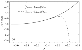
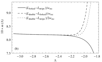
Figure 6: The ratios of the rectangle width $w_{\mathrm{rec}}$ to linear combinations of the stable perimeters that correspond, in the limit of negative $\Lambda$, to the constants (a) $c$ and (b) $m$.

Given this description, one might imagine that the perimeter of any simply connected domain with $n$ threefold junctions (and no junctions of higher order) will be,

$$L\simeq L_{\mathrm{rec}}+(c+mn)w_{\mathrm{rec}}$$ (30)

for $\Lambda$ sufficiently negative. This is a remarkably simple characterization of complicated domain structure, but, as we will see, it indeed holds for domains which resemble the intricate structure of those seen in experiment. Though this model necessarily restricts itself to domains with threefold junctions, recall that we only found stable shapes with threefold junctions. As it turns out, junctions of higher order are never seen in stable shapes in our numerics and rarely seen in experimental domains due to the vertex splitting instability, which highly disfavors vertex symmetries of fourfold symmetry and higher Cebers and Drikis (1996, 1999).

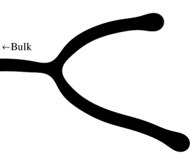
Figure 7: An example of two branches in a more complex branching domain.

Unfortunately, the stable domain structures seen in Fig. 4 lack many of the qualitative properties seen in experiment, e.g., branching structure, asymmetry, and snaking behavior. We suspect that this is because, in experimental settings, there is a nonzero effective background potential $V(\boldsymbol{\mathbf{r}})$. This could come from small inhomogeneities of the substrate, fringing or imperfect applied fields, etc. These imperfections can pin nearly stable domains. We can estimate the size of the potential needed for this pinning by considering two branches of a typical structure, like those in Fig. 7. Our analysis of the threefold harmonic shape suggests such a configuration is unstable and will decay by shortening one branch down into the other. We wish to find the energy gradient associated with this decay. Consider a small cross section of the upper branch and compute the energy it takes to move this piece onto the lower branch. Since such a move conserves the perimeter of the shape, the line tension and logarithmic terms in the energy do not change. The dipole energy of the small section with respect to the bulk scales like the area of the section, $w_{\mathrm{rec}}\cdot\Delta x$, over the cube of the mean distance of that section from the rest of material, which we expect to scale like $L_{\mathrm{rec}}$. There is a scaling constant $c_{1}$ that depends on the geometry of the bulk relative to the upper branch. Upon moving to the lower branch, the scaling behavior is identical, but the bulk relation constant changes to $c_{2}$. Therefore, we have

$$\Delta F=\frac{w_{\mathrm{rec}}\Delta x}{L_{\mathrm{rec}}^{3}}(c_{2}-c_{1})$$ (31)

Using the known scaling behavior of $L_{\mathrm{rec}}$ and $w_{\mathrm{rec}}$, this can be written

$$\frac{\Delta F}{\Delta x}\sim e^{4(\Lambda+1)}$$ (32)

Thus, as $\Lambda$ becomes negative, like it does in the regime where we see branching structures emerge, the energy gradient which destroys branching structures becomes smaller exponentially. In this regime, we should expect to see branching structures begin to emerge over random backgrounds of even modest amplitude.

The form of our random energy background is as follows. First, we choose positive real numbers $k_{0}$ and $a_{0}$ to characterize the scale of the noise and an integer $M$ to give the number of modes included. Then, we create a set of vectors $\{\boldsymbol{\mathbf{k}}_{i}\}$ and sets of scalars $\{a_{i}\}$ and $\{\phi_{i}\}$, where $i=1,\ldots M$. The $\boldsymbol{\mathbf{k}}_{i}$ are taken from a uniform distribution in the circle of radius $k_{0}$ centered at the origin, the $a_{i}$ are taken uniformly from the interval $[0,2a_{0}/M]$, and the $\phi_{i}$ are taken uniformly from the interval $[0,2\pi]$. The background energy is then given by the density

$$V(\boldsymbol{\mathbf{\rho}})=\sum_{i=1}^{M}a_{i}\cos(\boldsymbol{\mathbf{k}}_{i}\cdot\boldsymbol{\mathbf{\rho}}+\phi_{i}).$$ (33)

Consider the function $\boldsymbol{\mathbf{\Pi}}:\mathbb{R}^{2}\to\mathbb{R}^{2}$ defined by

$$\boldsymbol{\mathbf{\Pi}}(\boldsymbol{\mathbf{\rho}})=\frac{1}{2}\sum_{i=1}^{M}a_{i}\sin(\boldsymbol{\mathbf{k}}_{i}\cdot\boldsymbol{\mathbf{\rho}}+\phi_{i})\left[\frac{1}{k_{ix}},\;\frac{1}{k_{iy}}\right].$$ (34)

It follows that $\boldsymbol{\mathbf{\nabla}}\cdot\boldsymbol{\mathbf{\Pi}}=V$. This is precisely the condition we have on the external line potential $\boldsymbol{\mathbf{\Pi}}$. Therefore, the numerical approximation to the energy is given by

$$F_{\text{rand}}=\oint_{\partial\Omega}\boldsymbol{\mathbf{\Pi}}\cdot\hat{\boldsymbol{\mathbf{n}}}\,ds=\oint_{\partial\Omega}ds\;(\Pi_{x}\hat{n}_{x}+\Pi_{y}\hat{n}_{y})=\frac{1}{2}\oint_{\partial\Omega}\sum_{i=1}^{M}a_{i}\sin(\boldsymbol{\mathbf{k}}_{i}\cdot\boldsymbol{\mathbf{\rho}}+\phi_{i})\left(\frac{\hat{t}_{y}}{k_{ix}}-\frac{\hat{t}_{x}}{k_{iy}}\right)ds,$$ (35)

where we have used $\hat{n}_{x}=\hat{t}_{y}$ and $\hat{n}_{y}=-\hat{t}_{x}$, true for the tangents and normals of positively oriented domains. This means that, given the discretization of the domain boundary we used before,

$$F_{\text{rand}}=\frac{1}{2}\sum_{j=1}^{N}\sum_{i=1}^{M}a_{i}\sin(\boldsymbol{\mathbf{k}}_{i}\cdot\boldsymbol{\mathbf{\rho}}_{j}+\phi_{i})\left(\frac{y_{j+1}-x_{j}}{k_{ix}}-\frac{x_{j+1}-x_{j}}{k_{iy}}\right),$$ (36)

where the first sum is over the points making up the sides of the domain and the indices are defined cyclically. We can now simulate domains over such backgrounds in precisely the same way as we did in the case without the background.

With this modification, we are able to recover many of the qualitative features seen in experiment that were not seen for the minimizers we observe in the absence of noise. See, for instance, Fig. 8, which shows samples of these shapes at a variety of $\Lambda$ values and background intensities. Moreover, we found that the perimeters of these shapes continue to correspond, to a large degree, with the rectangle relationship $L_{\mathrm{rec}}(\Lambda)$ that we found before. In Fig. 9, we have plotted the perimeter of arbitrary shapes over a random background as a function of $\Lambda$. The color of each point corresponds to the intensity of the random background it was generated in. Notice first that the nature of the background does not seem to influence domain perimeter in a regular way. Next, notice that despite the relative complexity of these shapes, their perimeters remain very close to the rectangular idealization. However, there is an upward trend with increasing negative $\Lambda$.

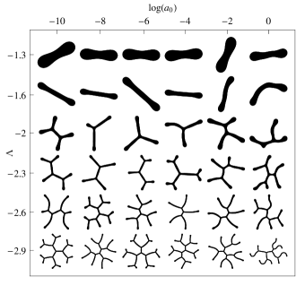
Figure 8: A sampling of stable solutions to our numeric model over random external potentials. Travelling down the vertical axis corresponds to decreasing $\Lambda$ and travelling to the right on the horizontal axis corresponds to increasing background intensity.

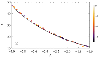
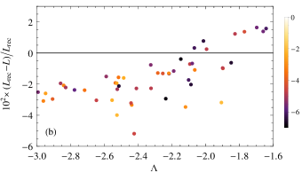
Figure 9: (Color online) The top plot shows the perimeter $L$ of stable domains as a function of $\Lambda$. The color of each point denotes the value of $\log_{10}(a_{0})$, the order of magnitude of the random background, as detailed by the legend. The solid black line is a plot of $L_{\mathrm{rec}}(\Lambda)$. The lower plot shows the relative error of each perimeter from $L_{\mathrm{rec}}$.

A similar upward trend exists in another shape-relevant morphological parameter: the number of junctions in the domain. This trend is shown in Fig. 10. Given the simple model (30), one would expect a greater number of junctions to correspondingly cause inflation in the observed perimeter from that of the rectangle. By inverting that model, we can make a prediction $\Lambda^{\prime}$ of a domain’s true value of $\Lambda$, i.e., that at which it was generated. This prediction is given by

$$\Lambda^{\prime}=\log\left[\frac{L-\sqrt{L^{2}-8\pi(c+mn)}}{2(c+mn)}\right]-1.$$ (37)

We tested this model at values of $\Lambda$ between $-3$ and $-1.6$ for sets of $50$ domains minimized over random backgrounds. Fig. 11 shows the error in those predictions. As can be seen there, for all $\Lambda$ tested the error in our model was less than 1%. The upward trend for $\Lambda\sim-3$ may be due to numerical under-resolution Kent-Dobias (2014).

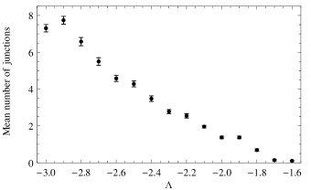
Figure 10: The average number of junctions in numeric domains as a function $\Lambda$. The error bars denote standard error.

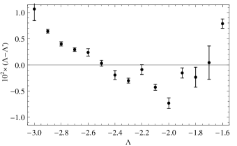
Figure 11: The difference between the generating value $\Lambda$ and the mean predicted value $\Lambda^{\prime}$ for sets of $50$ domains. The error bars denote standard error.

IV Conclusions

In this work, we have developed a way to express the energy of a dipole-mediated system that depends only on a single non-dimensional parameter, $\Lambda$. Numeric simulations using energy minimization were developed. We used these simulations to track the bifurcations of domains from a circle, and resolve subcritical branches for the first five harmonic bifurcations, and in particular for that of the circle to dogbone transition. Using the same methodology, we found three stable domain morphologies beyond the circle, all of which resemble a rectangular domain in appearance and behavior. Among these, the stripe, which evolves from a dogbone, is suspected to be the global energy minimizer in the unstable-circle regime.

The fact that these observed domains lack the qualitative features of experimental domains led to the conclusion that those features necessarily depend on the presence of an imperfect background energy landscape, and we confirmed this by recovering those features in our numerics. Using these domains, we found that a simple model suggested by the stable domains continues to work well in deriving the value of $\Lambda$ from the shape of an arbitrary domain. This model is especially powerful, because it only relies on the area-normalized perimeter and number of junctions present in the shape. These features can extracted from photographs of experiments, and so recovery of $\Lambda$, which contains ratios of physical variables, is straightforward in practice. An experimentalist could use this technique while varying some known parameter, e.g., the magnetic field or domain area, to work out other, unknown parameters by a fit of the system’s $\Lambda$-dependence. We hope to explore the possibility of our model being used in this way through collaboration with experimentalists.

V Acknowledgements

This work was done in part under NSF grants CBET-07306630 and DMS-1009633. The authors would like to thank Elizabeth Mann and David Jackson for the experimental images they generously contributed, the Mathematics and Biology departments of Harvey Mudd College for the use of their computing resources, and Professor Chad Higdon-Topaz for his support.

References

- Cebers (1980) A. Cebers, Magnetohydrodynamics 16, 236 (1980).
- Cebers and Maiorov (1980a) A. Cebers and M. Maiorov, Magnetohydrodynamics 16, 21 (1980a).
- Cebers and Mayorov (1980) A. Cebers and M. Mayorov, Magnetohydrodynamics 16, 231 (1980).
- Cebers and Maiorov (1980b) A. Cebers and M. Maiorov, Magnetohydrodynamics 16, 126 (1980b).
- Cebers and Zemitis (1983) A. Cebers and A. Zemitis, Magnetohydrodynamics 19, 360 (1983).
- McConnell and Moy (1988) H. M. McConnell and V. T. Moy, The Journal of Physical Chemistry 92, 4520 (1988), http://pubs.acs.org/doi/pdf/10.1021/j100326a053 .
- Vanderlick and Moehwald (1990) T. Vanderlick and H. Moehwald, Journal of Physical Chemistry 94, 886 (1990).
- McConnell (1990) H. M. McConnell, Journal of Physical Chemistry 94, 4728 (1990).
- McConnell and de Koker (1992) H. M. McConnell and R. de Koker, The Journal of Physical Chemistry 96, 7101 (1992).
- Langer et al. (1992) S. A. Langer, R. E. Goldstein, and D. P. Jackson, Physical Review A 46, 4894 (1992).
- Dickstein et al. (1993) A. J. Dickstein, S. Erramilli, R. E. Goldstein, D. P. Jackson, and S. A. Langer, Science 261, 1012 (1993), http://www.sciencemag.org/content/261/5124/1012.full.pdf .
- Goldstein and Jackson (1994) R. E. Goldstein and D. P. Jackson, The Journal of Physical Chemistry 98, 9626 (1994).
- Jackson et al. (1994) D. P. Jackson, R. E. Goldstein, and A. O. Cebers, Physical Review E 50, 298 (1994).
- de Koker and McConnell (1994) R. de Koker and H. M. McConnell, The Journal of Physical Chemistry 98, 5389 (1994).
- de Koker et al. (1995) R. de Koker, W. Jiang, and H. M. McConnell, The Journal of Physical Chemistry 99, 6251 (1995).
- Lubensky and Goldstein (1996) D. K. Lubensky and R. E. Goldstein, Physics of Fluids (1994-present) 8, 843 (1996).
- Seul and Andelman (1995) M. Seul and D. Andelman, Science 267, 476 (1995).
- McConnell and de Koker (1996) H. M. McConnell and R. de Koker, Langmuir 12, 4897 (1996).
- Cebers and Drikis (1996) A. Cebers and I. Drikis, Magnetohydrodynamics 32, 8 (1996).
- Cebers and Drikis (1999) A. Cebers and I. Drikis, in Free Boundary Problems: theory and applications, Vol. 409, edited by I. Athanasopoulos, J. F. Rodrigues, and G. Makrakis (CRC Press, 1999) pp. 14–38.
- Mann and Primak (1999) E. K. Mann and S. V. Primak, Physical Review Letters 83, 5397 (1999).
- Khattari and Fischer (2002) Z. Khattari and T. M. Fischer, The Journal of Physical Chemistry B 106, 1677 (2002).
- Elias et al. (1998) F. Elias, I. Drikis, A. Cebers, C. Flament, and J.-C. Bacri, The European Physical Journal B-Condensed Matter and Complex Systems 3, 203 (1998).
- Otto (1998) F. Otto, Archive for Rational Mechanics and Analysis 141, 63 (1998).
- Heinig et al. (2004) P. Heinig, L. E. Helseth, and T. M. Fischer, New Journal of Physics 6, 189 (2004).
- Hillier and Jackson (2007) N. J. Hillier and D. P. Jackson, Physical Review E 75, 036314 (2007).
- Jackson (2008) D. P. Jackson, Journal of Physics: Condensed Matter 20, 204140 (2008).
- Alexander et al. (2007) J. C. Alexander, A. J. Bernoff, E. K. Mann, J. A. Mann, J. R. Wintersmith, and L. Zou, Journal of Fluid Mechanics 571, 191 (2007).
- Tucker (2008) G. Tucker, Harvey Mudd College Senior Theses (2008).
- de Koker and McConnell (1993) R. de Koker and H. M. McConnell, The Journal of Physical Chemistry 97, 13419 (1993), http://pubs.acs.org/doi/pdf/10.1021/j100152a057 .
- Kent-Dobias (2014) J. Kent-Dobias, Harvey Mudd College Senior Theses (2014).
- Hansen and McDonald (1990) J.-P. Hansen and I. R. McDonald, Theory of simple liquids (Elsevier, 1990).
- Bertsekas (1999) D. P. Bertsekas, Nonlinear Programming, 2nd ed. (Athena Scientific, Belmont, MA, 1999).