A Very Simple Cusped Halo Model

Abstract

We introduce a very simple model of a dark halo. It is a close relative of Hernquist’s model, being generated by the same transformation but this time applied to the logarithmic potential rather than the point mass. The density is proportiional to (distance)^-1 at small radii, whilst the rotation curve is flat at large radii. Isotropic and radially anisotropic distributions functions are readily found, and the intrinsic and line of sight kinematical quantities are available as simple formulae. We also provide an analytical approximation to the Hamiltonian as a function of the actions. As an application, we study the kinematic properties of stellar haloes and tracers in elliptical galaxies. We show that the radial velocity dispersion of a power-law population in a galaxy with a flat rotation curve always tends to the constant value. This holds true irrespective of the anisotropy or the lengthscales of the dark or luminous matter. An analogous result holds for the line of sight or projected velocity dispersion of a power-law surface brightness profile. The radial velocity dispersion of Population II stars in the Milky Way is a strongly declining function of Galactocentric radius. So, if the rotation curve is flat, we conclude that the stellar halo density cannot follow a power-law at large radii, but must decrease more sharply (like an Einasto profile) or be abruptly truncated at large radii. Both the starcount and kinematic data of the Milky Way stellar halo are well-represented by an Einasto profile with index $m\approx 2$ and effective radius $\approx 20$ kpc.

1 INTRODUCTION

Hernquist (1990) devised a very simple spherical model with potential- density pair

$$\psi = {GM\over r+a},$$

$$\rho = {M\over 2\pi}{a\over r(r+a)^{3}}.$$ (1)

Here $M$ is the mass of the model and $a$ is a scalelength related to the half mass radius. Hernquist’s model provides a beguiling combination of simplicity and realism. It has become well-known as a representation of elliptical galaxies and bulges. It has also become widely used in $N$ body calculations, as the forces are analytic and so ease numerical orbit integrations. We note that the model is obtained from the familiar Keplerian potential of a point mass by the straightforward transformation $r\rightarrow r+a$.

Here, we will provide a very simple spherical model of a galaxy with a flat rotation curve generated by the exact same transformation – but this time applied to the logarithmic potential of the singular isothermal sphere. This gives the potential-density pair

$$\psi = -v_{0}^{2}\log(r+a)+{\rm constant},$$

$$\rho = {v_{0}^{2}\over 4\pi G}{2a+r\over r(r+a)^{2}}.$$ (2)

The similarity with Hernquist’s original model is evident. Henceforth, we choose the constant as $v_{0}^{2}\log a$ so that the potential $\psi$ is zero at the centre.

The model has an asymptotically flat rotation curve. But – like Hernquist’s model – it has a $1/r$ cusp in the density. This is of course highly desirable given the findings of Navarro, Frenk & White (1996) that galaxy formation via hierarchical merging in a cold dark matter (CDM) dominated universe gives rise to density cusps of the form $\rho\propto 1/r$ at small radii. The NFW profile probably does not describe the haloes of large galaxies like the Milky Way or M31 (e.g., Binney & Evans 2001) or small dwarf irregulars and spheroidals (e.g., Oh et al. 2008; Agnello & Evans 2012). This is thought to be the result of baryonic processes that may modify the central regions (e.g., Pontzen & Governato 2014). Nonetheless, models with $1/r$ density cusps are still invaluable as an approximation to equilibrium configurations of dark matter in dissipationless simulations.

In Section 2, we describe the properties of our new halo model (2), providing formulae for the kinematic quantities, distribution functions and actions. Section 3 looks at the properties of tracer populations with an eye on the kinematics of stellar haloes and elliptical galaxies. Section 4 sums up, comparing our halo model with a number of familiar faces from the literature.

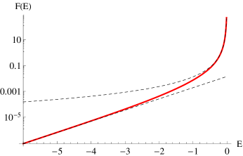
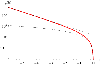
Figure 1: Distribution function $f$ and density of states $g$ as a function of binding energy $E$ for the isotropic model ($v_{0}=1=a=G$). The full results are shown in red, whilst the asymptotic and cusp approximations are shown as dashed lines.

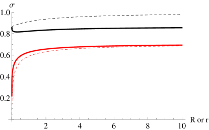
Figure 2: Radial (dashed) and line of sight (unbroken) velocity dispersion as a function of intrinsic radius $r$ and projected radius $R$ respectively. The isotropic model ($\beta=0$) is shown in red and the radially anisotropic model ($\beta=1/2$) in black. Note that the line of sight velocity distribution picks up contributions from the tangential velocity dispersion, and so the full line lies above the dashed for the isotropic model, but below the dashed for the radially anisotropic model. Units are chosen so that $v_{0}=a=1$.

2 Properties of the Model

First, we will derive some properties of the self-consistent model. Our results apply to the total (baryonic plus dark matter) content of the galaxy.

2.1 Preliminaries

The phase space distribution function (henceforth DF) is of fundamental dynamical importance. By Jeans (1919) theorem, the DF is a function of the isolating integrals of motion only. As the model is spherical, the DF may depend on the binding energy per unit mass $E$ and the modulus of the angular momentum $L$

$$E = -\tfrac{1}{2}(v_{r}^{2}+v_{\theta}^{2}+v_{\phi}^{2})-v_{0}^{2}\log(1+r/a),$$

$$L^{2} = r^{2}(v_{\theta}^{2}+v_{\phi}^{2}).$$ (3)

Isotropic DFs depend only on $E$, whereas anisotropic DFs depend on $L$ as well.

We look for DFs in which the anisotropy parameter

$$\beta=1-{\langle v_{\theta}^{2}\rangle\over\langle v_{r}^{2}\rangle},$$ (4)

takes a constant value. Of course, for a spherical density distribution in a spherical potential, it must be the case that $\langle v_{\phi}^{2}\rangle=\langle v_{\theta}^{2}\rangle$. The parameter $\beta$ may take values in the range $-\infty\leq\beta\leq 1$. The isotropic model corresponds to the case $\beta=0$. Models with $\beta>0$ are radially anisotropic with $\beta\rightarrow 1$ being the radial orbit model. Models with $\beta<0$ are tangentially anisotropic with $\beta\rightarrow-\infty$ being the circular orbit model.

The DF of a spherical system with constant anisotropy is

$$f(E,L)=L^{-2\beta}f_{E}(E).$$ (5)

The unknown function $f_{E}(E)$ can be recovered from the integral inversion formula (e.g., Wilkinson & Evans 1999, Evans & An 2006)

$$f_{E}(E)=\frac{2^{\beta}(2\pi)^{-3/2}}{\Gamma(1-\lambda)\Gamma(1-\beta)}\ \frac{d}{dE}\!\int_{0}^{E}\frac{d\psi}{(E-\psi)^{\lambda}}\frac{d^{n}h}{d\psi^{n}}$$ (6)

where $h=r^{2\beta}\rho$ is expressed as a function of $\psi$, and $n=\lfloor(3/2-\beta)\rfloor$ and $\lambda=3/2-\beta-n$ are the integer floor and the fractional part of $3/2-\beta$. This includes Eddington’s (1916) formula for the isotropic DF as a special case ($\beta=0$).

If $\beta$ is a half-integer constant (i.e., $\beta=$ $1/2$, $-1/2$, and so on), the expression for DF further reduces to

$$f(E,L)=\frac{1}{2\pi^{2}}\frac{L^{-2\beta}}{(-2\beta)!!}\ \left.\frac{d^{3/2-\beta}h}{d\psi^{3/2-\beta}}\right|_{\psi=E}.$$ (7)

Rather remarkably, this involves only differentiations. The expression for the differential energy distribution is

$$\frac{dM}{dE}=f_{E}(E)g(E)\,$$ (8)

where the density of states $g(E)$ is

$$g(E)=\frac{(2\pi)^{5/2}\Gamma(1-\beta)}{2^{\beta-1}\Gamma(3/2-\beta)}\int_{0}^{r_{E}}(\psi-E)^{1/2-\beta}r^{2(1-\beta)}dr,$$ (9)

generalizing the formula in Binney & Tremaine (2008) for the isotropic case. Here, $r_{E}$ is the radius of the largest orbit of a particle with energy $E$, that is to say, $\psi(r_{E})=E$.

2.2 Distribution Functions

The key to the simplicity of our model is that $\psi(r)$ can be easily inverted to give $r(\psi)$, namely

$$r=a\exp(-\psi/v_{0}^{2})-a.$$ (10)

This means that $\rho(\psi)$ can also be easily constructed.

$$\rho(\psi)={v_{0}^{2}\over 4\pi Ga^{2}}{\exp(2\psi/v_{0}^{2})+\exp(3\psi/v_{0}^{2})\over 1-\exp(\psi/v_{0}^{2})}.$$ (11)

The general constant anisotropy DF can be found using eq. (6) as

$$F(E,L)=AL^{-2\beta}\exp((2-2\beta)E/v_{0}^{2})\left[1+\sum_{j=1}^{\infty}C_{j}\exp(jE/v_{0}^{2})\right],$$ (12)

where the constants $A$ and $C_{j}$ are defined in the Appendix. Note that the DF is only positive definite if $\beta\leq 1/2$. If $\beta$ exceeds this value, the DF is negative at the centre. This is in accord with the cusp-anisotropy theorem of An & Evans (2005), which states that in spherical symmetry models with a cusp like $r^{-\gamma}$ at the centre must satisfy $\beta\leq 2\gamma$.

The asymptotic forms of the DF in the cusp ($r\ll a$) and in the outer parts ($r\gg a$) are a power-law in energy or an exponential in energy respectively:

$${F_{\rm cusp}}(E,L) = {v_{0}^{4-4\beta}\Gamma(5/2-3\beta)\over 2^{5/2-\beta}Ga^{2-2\beta}L^{2\beta}\Gamma(1-\beta)\Gamma(2-2\beta)}(-E)^{-5/2+3\beta}$$

$${F_{\rm asym}}(E,L) = AL^{2\beta}\exp(2-2\beta)E/v_{0}^{2}.$$ (13)

2.3 Special Cases: Isotropy and Radial Anisotropy

When $\beta=0$, the isotropic DF is an infinite sum of exponentials

$$F(E)={\exp(2E/v_{0}^{2})\over 4\pi^{5/2}Gv_{0}a^{2}}\left[1+2^{-1/2}\sum_{j=1}^{\infty}(2+j)^{3/2}\exp(jE/v_{0}^{2})\right].$$ (14)

The density of states is

$$g(E) = 8a^{3}v_{0}\pi^{5/2}\Biggl{[}\sqrt{2}Y(E/v_{0}^{2})-Y(2E/v_{0}^{2})$$ (15)

$$+ {\sqrt{2}\over 3\sqrt{3}}Y(3E/v_{0}^{2})-{2\over 3}\sqrt{{-2E\over\pi v_{0}^{2}}}\Biggr{]},$$

where $Y(s)=\exp(-s){\rm erf}(\sqrt{-s})$. Again, we can develop simple approximations valid for the far-field and the cusp, namely

$${g_{\rm cusp}}(E) = {256\sqrt{2}\over 105}{\pi^{2}a^{3}\over v_{0}^{6}}(-E)^{7/2},$$ (16)

$${g_{\rm asym}}(E) = {8\sqrt{2}\over 3\sqrt{3}}\pi^{5/2}v_{0}a^{3}\exp(-3E/v_{0}^{2}).$$ (17)

Plots of the isotropic distribution function and density of states are shown in Fig. 1, together with the approximations that hold good in the cusp and in the far-field.

The isotropic ($\beta=0$) velocity dispersions are

$$\langle v_{r}^{2}\rangle=\langle v_{\theta}^{2}\rangle=\langle v_{\phi}^{2}\rangle={v_{0}^{2}\over 2}\,{4r(a+r)^{2}\log\left(1+r/a\right)-ar(5a+4r)\over a^{2}(2a+r)}.$$ (18)

As $r\rightarrow 0$, the velocity dispersions tend to zero, whilst as $r\rightarrow\infty$, the velocity dispersions tend to $v_{0}/\sqrt{2}$.

When $\beta=1/2$, the DF is particularly simple, as the infinite series reduces to just two terms. (In fact, whenever $\beta$ is a half-integer, the DF has a simple closed form). We find that

$$F(E,L)={1\over 8\pi^{3}Ga|L|}\left[\exp(E/v_{0}^{2})+2\exp(2E/v_{0}^{2})\right].$$ (19)

This is analogous to the very simple DF for the Hernquist model (Baes & Dejonghe 2002, Evans & An 2005). Evidence from numerical simulations suggests that the velocity distribution of the dark matter is radially anisotropic with $\beta\approx 1/2$ (e.g., Hansen & Moore 2006), so this is a cosmologically realistic DF. The density of states is

$$g(E)=4\pi^{3}a^{2}(\exp(-E/v_{0}^{2})-1)^{2}.$$ (20)

For the radially anisotropic ($\beta=1/2$) model, the velocity dispersions are

$$\langle v_{r}^{2}\rangle={v_{0}^{2}\over 2}{3a+2r\over 2a+r},\qquad\langle v_{\theta}^{2}\rangle=\langle v_{\phi}^{2}\rangle={v_{0}^{2}\over 4}{3a+2r\over 2a+r}.$$ (21)

As $r\rightarrow 0$, the radial velocity dispersion tends to $\sqrt{3}v_{0}/2$, whilst as $r\rightarrow\infty$, it tends to $v_{0}$.

Let us check that our models obey the virial theorem. In both cases, the potential energy is

$$\Omega(r) = 4\pi\int_{0}^{r}r^{3}\rho{d\psi\over dr}dr$$

$$= -{v_{0}^{4}\over 2G(a+r)^{2}}\left[r(2a^{2}+3ar+2r^{2})-2a(a+r)^{2}\log(1+r/a)\right].$$

The kinetic energy of the isotropic ($\beta=0$) model is

$$T(r) = 6\pi\int_{0}^{r}r^{2}\rho\langle v_{r}^{2}\rangle dr={v_{0}^{4}\over 4Ga^{2}(a+r)}\left[ar(2a^{2}+ar-4r^{2})\right.$$ (23)

$$+ 4(a+r)r^{3}\log(1+a/r)-\left.2(a+r)a^{3}\log(1+r/a)\right],$$

so that, as $r\rightarrow\infty$, $T\rightarrow 3v_{0}^{4}r/(4G)$ and $\Omega\rightarrow-v_{0}^{4}r/G$.

By contrast, the kinetic energy of the radially anisotropic ($\beta=1/2$) model is

$$T(r) = (6-4\beta)\pi\int_{0}^{r}r^{2}\rho\langle v_{r}^{2}\rangle dr$$ (24)

$$= {v_{0}^{4}\over 2G(a+r)}\left[r(a+2r)-a(a+r)\log(1+r/a)\right]$$

so that, as $r\rightarrow\infty$, $T\rightarrow v_{0}^{4}r/G$.

The virial theorem reads

$${2T(r)+\Omega(r)}=4\pi r^{3}\rho\langle v_{r}^{2}\rangle.$$ (25)

As $r\rightarrow\infty$, the virial theorem does not take its familiar form, but instead:

$$2T+\Omega\rightarrow\begin{cases}{v_{0}^{4}r\over 2G},&\mbox{if }\beta=0,\\ {v_{0}^{4}r\over G},&\mbox{if }\beta=1/2.\end{cases}$$ (26)

Just like the isothermal sphere, the models do not obey the virial theorem unless the surface term is included.

2.4 Projected and Line of Sight Quantities

The projected surface density $\Sigma(s)$ is best written as

$$\Sigma(R)={v_{0}^{2}\over 2\pi Ga(s^{2}-1)}(1+(s^{2}-2)X(s)).$$ (27)

Here, $s=R/a$, and, following Hernquist (1990), we have used the notation

$$X(s)=\begin{cases}{\displaystyle{1\over\sqrt{1-s^{2}}}{\rm arcsech}s},&0\leq s\leq 1,\\ {\displaystyle{1\over\sqrt{s^{2}-1}}{\rm arcsec}s},&s\geq 1.\end{cases}$$

Note that $X(1)=1$.

At the centre, $\Sigma(R)$ diverges logarithmically, whereas it falls like $1/R$ at large radii, viz.,

$$\Sigma_{\rm cusp}(R) = {v_{0}^{2}\over\pi Ga}\log\left({2a\over R}\right),$$

$$\Sigma_{\rm asym}(R) = {v_{0}^{2}\over 4G}{1\over R}.$$ (28)

The line of sight or projected velocity dispersion of the isotropic model ($\beta=0$) is

$$\langle v_{\rm los}^{2}\rangle = {2\over\Sigma(R)}\int_{R}^{\infty}\rho\langle v_{r}^{2}\rangle{rdr\over\sqrt{R^{2}-r^{2}}}$$ (29)

$$= {v_{0}^{2}\over 2}{(4s^{2}+2\pi s-3-2\pi s^{3})+s^{2}(4s^{2}-5)X(s)\over 1+(s^{2}-2)X(s)}$$

which tends to $v_{0}/\sqrt{2}$ at large radii. At small radii, the projected velocity dispersion tends to zero logarithmically

$$\langle v_{\rm los}^{2}\rangle\rightarrow{3v_{0}^{2}\over 4}{1\over\log(2a/R)}$$ (30)

Finally, the line of sight velocity dispersion of the radially anisotropic ($\beta=1/2$) model is

$$\langle v_{\rm los}^{2}\rangle = {2\over\Sigma(R)}\int_{R}^{\infty}\rho\langle v_{r}^{2}\rangle\left(1-{R^{2}\over 2r^{2}}\right){rdr\over\sqrt{R^{2}-r^{2}}}$$

$$= {v_{0}^{2}\over 4}{(5+2\pi s^{\textsterling}-4s^{2}-2\pi s)-(6-9s^{2}+4s^{4})X(s)\over 1+(s^{2}-2)X(s)}$$

At both small and large radii, the velocity dispersion tends to the value $\sqrt{3}v_{0}/2$. The intrinsic and line of sight velocity dispersions are shown in Fig. 2.

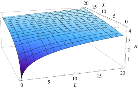
Figure 3: A surface plot of $\mathcal{H}$ for the case $a=v_{0}=1$.

2.5 The Hamiltonian and the Actions

Action-angles are an extremely useful set of coordinates in which to visualize the form of a Hamiltonian. Since actions are integrals of motion, they automatically satisfy $\dot{J_{i}}=0$, and the canonically conjugate angle variables evolve in time in a trivial fashion:

$$\theta_{i}(t)=\theta_{i}(0)+\Omega_{i}t,\qquad\qquad\Omega_{i}=\frac{\partial H}{\partial J_{i}}.$$ (32)

In a spherical potential, the radial action $J_{r}$ is:

$$J_{r}=\oint\sqrt{2\psi-2E-L^{2}/r^{2}}\mathrm{d}r,.$$ (33)

The angular actions are related to the angular momentum components via $J_{\phi}=L_{z}$ and $J_{\theta}=L-L_{z}$, where $L$ is given by eq. (3), whilst $L_{z}$ is the angular momentum about the $z$-axis. We then have a complete set of canonical coordinates when the actions are complemented by their respective angles. In the spherical case, the Hamiltonian can then be regarded as a function of just two quantities: $H\equiv H(L,J_{r})$ (see Binney & Tremaine 2008). However, due to the difficulty in evaluating the integral in equation (33), we cannot generally find $J_{r}(E,L)$ and therefore $H(L,J_{r})$. In fact, Evans, Lynden-Bell & de Zeeuw (1990) showed that the most general potential for which the actions are available as elementary functions is the isochrone.

For our model, it is therefore no surprise that $J_{r}(E,L)$ and $L(E,J_{r})$ cannot be found in the general case. However, progress can be made by using the approximations found in Williams, Evans & Bowden (2014) (hereafter WEB). The method described in WEB approximates $H(L,J_{r})$ for scale-free spherical potentials by calculating the energy of purely radial orbits

$$J_{r}=\dfrac{1}{2\pi}\oint\sqrt{2\psi(r)-2E(0,J_{r})}\mathrm{d}r,$$ (34)

and of circular orbits

$$L(r)=rv_{\rm c}(r),\qquad\qquad E(L,0)=\psi(r)-\frac{1}{2}v_{\rm c}(r)^{2}.$$ (35)

Each of these equations gives a solution with the same functional form, $-E(J_{i},J_{j}=0)=f(a_{i}J_{i})$, and WEB create an approximate Hamiltonian by analytically interpolating between these two limiting cases in a very simple way, so that

$$\mathcal{H}(L,J_{r})=f(aL+bJ_{r}).$$ (36)

Of course, the potential considered here is spherically symmetric but not scale free. For example, the radial action of a general radial orbit is given by

$$J_{r}=\frac{\sqrt{2}av_{0}}{\pi}\exp(-E/v_{0}^{2})\gamma(3/2,-E/v_{0}^{2}),$$ (37)

where $\gamma(s,x)$ is the lower incomplete gamma function. This integral equation cannot be solved in the general case, so we look to find specific solutions in the limiting cases. The obvious limits to consider are orbits in the cusp of the model ($r\ll a$) and orbits in the outer halo ($r\gg a$). Using these limiting cases, we can then use analytical interpolation to find a function $\mathcal{H}$ that well approximates the true Hamiltonian $H$ everywhere in action space.

2.5.1 The Cusp

In the cusp of the potential ($r\ll a$), we Taylor expand the potential as

$$\psi(r)=-\dfrac{v_{0}^{2}r}{a}+\mathcal{O}(r^{2}),$$ (38)

demonstrating that the potential is a scale-free power-law potential in this regime. As a result, we can employ the results from WEB to find an accurate analytical form for $H_{\mathrm{cusp}}(L,J_{r})$. We use their equation (12) with $\alpha=1$ to find

$$\mathcal{H}_{\mathrm{cusp}}(L,J_{r})=\dfrac{3v_{0}^{4/3}}{2a^{2/3}}\bigg{(}L+\frac{\pi}{\sqrt{3}}J_{r}\bigg{)}^{2/3}.$$ (39)

For a more accurate result, we can employ the first-order corrected version of this formula to give

$$\mathcal{H}_{\mathrm{cusp}}(L,J_{r})=\dfrac{3v_{0}^{4/3}}{2a^{2/3}}\bigg{(}L+\frac{\pi}{\sqrt{3}}J_{r}+\epsilon\sqrt{LJ_{r}}\bigg{)}^{2/3},$$ (40)

where $\epsilon=-0.0412$. This approximation is valid for orbits that spend the majority of their time in the region in the cusp regime. Numerically, we find that this corresponds to $|\boldsymbol{J}|=\sqrt{L^{2}+J_{r}^{2}}\lesssim 0.06av_{0}$. Given this expression for the Hamiltonian, we may then approximate the distribution function in this region of phase space by substituting $\mathcal{H}_{\mathrm{cusp}}$ into equation (13):

$${F_{\rm cusp}}(L,J_{r})=\mathcal{N}L^{2\beta}\bigg{(}L+\frac{\pi}{\sqrt{3}}J_{r}+\epsilon\sqrt{LJ_{r}}\bigg{)}^{-5/3+2\beta},$$ (41)

where $\mathcal{N}$ is the normalisation factor.

2.5.2 The Far-Field

If we instead consider the case when $r\gg a$, then the potential takes the form

$$\psi(r)\simeq-v_{0}^{2}\log r/a,$$ (42)

so this potential coincides with the singular isothermal sphere at large radii. In this case, the approximate Hamiltonian is given by

$$\mathcal{H}_{\mathrm{asym}}(L,J_{r})=v_{0}^{2}\log\bigg{(}\dfrac{\sqrt{e}L+\sqrt{2\pi}J_{r}}{av_{0}}\bigg{)}.$$ (43)

As in the cusp, we can also improve this approximation if need be. The first-order corrected formula is

$$\mathcal{H}_{\mathrm{asym}}(L,J_{r})=v_{0}^{2}\log\bigg{(}\dfrac{\sqrt{e}L+\sqrt{2\pi}J_{r}+\epsilon\sqrt{LJ_{r}}}{av_{0}}\bigg{)}$$ (44)

with $\epsilon=-0.1009$. If we insert this expression into the far-field limit of the distribution function in eqn (13), we find

$${F_{\rm asym}}(L,J_{r})=\mathcal{M}L^{2\beta}\bigg{(}\sqrt{e}L+\sqrt{2\pi}J_{r}+\epsilon\sqrt{LJ_{r}}\bigg{)}^{2-2\beta},$$ (45)

where $\mathcal{M}$ is again the normalisation factor. Hence, we have shown that, in both the cusp and outer halo of this potential, the distribution function as a function of the actions is well approximated by a simple power law.

2.5.3 Generalisation to all action space

Now that we know the functional forms of $\mathcal{H}_{\mathrm{cusp}}$ and $\mathcal{H}_{\mathrm{asym}}$, we are in a position to construct a function ${\mathcal{H}}$ that approximates the full Hamiltonian $H$ everywhere in action space. Consider the following function

$${\mathcal{H}}(L,J_{r})=\dfrac{3v_{0}^{2}}{2}\log\left(1+\left(\dfrac{A(L)L+B(J_{r})J_{r}}{av_{0}}\right)^{2/3}\right)$$ (46)

where

$$A(L)=\dfrac{\sqrt{e}L+av_{0}}{L+av_{0}}\quad;\quad B(J_{r})=\dfrac{\sqrt{6\pi}J_{r}+\pi av_{0}}{\sqrt{3}(J_{r}+av_{0})}.$$ (47)

If we evaluate ${\mathcal{H}}(L,J_{r})$ in the limits $|\boldsymbol{J}|<<av_{0}$ and $|\boldsymbol{J}|>>av_{0}$, we find:

$${\mathcal{H}}(L,J_{r})=\begin{cases}\dfrac{3v_{0}^{4/3}}{2a^{2/3}}\bigg{(}L+\dfrac{\pi}{\sqrt{3}}J_{r}\bigg{)}^{2/3}\quad|\boldsymbol{J}|<<av_{0},\\ \\ v_{0}^{2}\log\bigg{(}\dfrac{\sqrt{e}L+\sqrt{2\pi}J_{r}}{av_{0}}\bigg{)}\quad|\boldsymbol{J}|>>av_{0}.\end{cases}$$ (48)

Hence, we find that ${\mathcal{H}}$ coincides with ${\mathcal{H}_{\mathrm{cusp}}}$ and ${\mathcal{H}_{\mathrm{asym}}}$ in the corresponding limits. The appearance of ${\mathcal{H}}$ can be seen in Figure 3. To test the accuracy of this approximation, we generated a finely spaced grid in action space, with $0\leq|\boldsymbol{J}|\leq 30av_{0}$. We find that the maximum absolute error on our grid is 5.48 percent, and the mean error is 1.61 percent. Predictably, the errors are largest in the regime $|\boldsymbol{J}|\sim av_{0}$, in which we transit between ${\mathcal{H}_{\mathrm{cusp}}}$ and ${\mathcal{H}_{\mathrm{asym}}}$, and lowest in the regimes where ${\mathcal{H}_{\mathrm{cusp}}}$ and ${\mathcal{H}_{\mathrm{asym}}}$ apply. The error distribution for the region $0\leq|\boldsymbol{J}|\leq 10av_{0}$ is given in Fig. 4, where one can clearly see that the error is worst close the the $L$–axis. This suggests that a correction term in $L$ might be prudent in eq. (46).

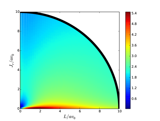
Figure 4: Distribution of absolute percentage error in $H$ in the region $0\leq|\boldsymbol{J}|\leq 10av_{0}$. One can see that the error peaks at $\sim 5$ percent close to the $L$–axis.

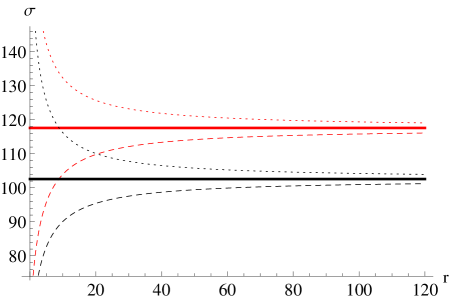
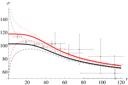
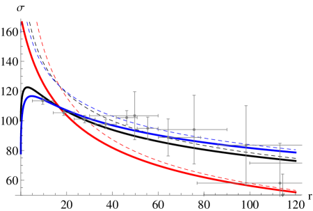
Figure 5: Radial velocity dispersion (in kms${-1}$) as a function of spherical polar radius $r$ (in kpc). Upper panel: When the rotation curve is flat, the radial velocity dispersion of an asymptotically power-law population is constant, as shown for $n=3.5$ (red) and $n=4.6$ (black). If the lengthscales of the dark matter is greater than (less than) that of the luminous matter, then the constant value is approached from below (above), as shown by the dashed (dotted) lines. Middle panel: The power-law densities are now modulated by a taper function that causes exponential decline beyond the taper radius ${r_{\rm t}}$, as in eq. (51). The effect of truncation of the density of the stellar population causes the isotropic velocity dispersion to decline. The colour coding is the same as in the upper panel, and the truncation parameters are ${r_{\rm t}}=40$ kpc and $p=10$. In this and the following panel, the datapoints of Deason et al. (2012) are overplotted in grey. Lower panel: The populations have Einasto profiles with an effective radius ${R_{\rm e}}=20$ kpc and isotropic velocity distributions. Red, black and blue curves refer to Einasto indices of 1, 1.7 and 2 respectively. Full (dashed) curves denote the case when the dark matter lengthscale $a$ is 1 (7.5) kpc. An Einasto model with $m=2$ and ${R_{\rm e}}=20$ kpc gives a good description of Deason et al’s data out to $\sim 110$ kpc.

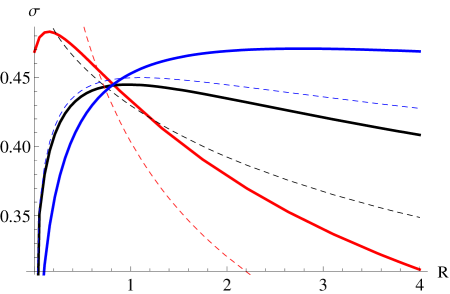
Figure 6: Line of sight velocity dispersion (in units of $v_{0}$) versus projected radius (in units of effective radius $R_{\rm e}$) for Sersic tracers. The isotropic cases are shown as thick lines, the radial anisotorpic cases as dotted. The models vary from exponential or $m=1$ (red), $m=2$ (black) to de Vaucouleurs or $m=4$ (blue).

3 Tracer Populations

So far, we have given properties of the self-consistent model. From the point of view of comparison with observational data, it is interesting to look at the properties of tracer populations. These might represent the stellar halos of disc galaxies or even entire elliptical galaxies embedded in a dark halo. In what follows, the total potential (dark matter and baryons) is always described by eq. (2), whilst the kinematic properties of the baryons are deduced from their light profiles using the Jeans equations.

3.1 Stellar Haloes

First, let us assume the stars follow the density-law

$$\rho_{\star}={\rho_{0}b^{n}\over(b+r)^{n}}.$$ (49)

Here, $b$ is the lengthscale of the luminous matter, as compared to $a$ which is the lengthscale in the potential, and hence of the dark matter. Power-laws are often used to describe populations in stellar haloes. Traditionally, in our own Galaxy, the density of Population II stars has often been described as a power-law with $n\approx 3.5$ (e.g., Freeman 1987). However, recent studies tend to find a faster fall-off (e.g., Watkins et al. 2009, Sesar et al. 2011). For example, using blue horizontal branch and blue straggler stars extracted from the Sloan Digital Sky Survey data, Deason et al. (2011) showed that the stellar halo is well fitted by a power-law with $n\approx 4.6$ for Galactocentric radii beyond $\approx 27$ kpc. Re-visiting the problem with Sloan Data Releases 9, Deason et al. (2014) argue that an even steeper power-law slope ($n\sim 6-10$) is favoured at larger radii ($r\sim 50-100$ kpc).

When $a=b$, the isotropic ($\beta=0$) distribution function of the stars is an isothermal and therefore the velocity distribution is a Gaussian with dispersion $v_{0}/\sqrt{n}$. This property of isothermals was already known to Smart (1938). More generally, for arbitrary anisotropy $\beta$ and arbitrary lengthscales for the dark and luminous matter $a$ and $b$, we can derive the asymptotic result

$$\langle v_{r}^{2}\rangle={v_{0}\over\sqrt{n-\beta}}\left[1+{n(b-a)+a\beta\over 2(n+1-\beta)}{1\over r}\right].$$ (50)

The radial velocity dispersion of an asymptotically power-law population in a galaxy with a flat rotation-curve always tends to a constant value. This finding is unaffected by velocity anisotropy $\beta$, which simply changes the constant asymptotic value to $v_{0}/\sqrt{n-\beta}$. For the isotropic case, the radial velocity dispersion reaches its asymptotic value from above (below) according to whether the lengthscale of the dark matter is less than (greater than) the lengthscale of the luminous matter. This can be deduced from eq (50) and is illustrated in the upper panel of Fig. 5.

However, this is very different to the behaviour of the radial velocity dispersion of populations in our own Galaxy’s halo. Deason et al. (2012) show that the radial velocity dispersion at 100 kpc has fallen to at least 40 per cent of its central value (see their Figure 9). If the rotation curve is flat, then it immediately follows that the stellar halo cannot have any power-law decline, but must fall off much more abruptly. This is because there is no sign in the data of a velocity dispersion tending to a constant value, at least within 100 kpc.

To illustrate this, let us consider truncated power-laws of the form

$$\rho_{\star}={\rho_{0}b^{n}\over(b+r)^{n}}\Biggl{[}1-\tanh^{p}(r/{r_{\rm t}})\Biggr{]}.$$ (51)

Here, ${r_{\rm t}}$ is a truncation radius. For $r\ll{r_{\rm t}}$, the tracer density has a power-law decline, but for $r\gg{r_{\rm t}}$ the power-law is modulated by a faster exponential decline with scalelength ${r_{\rm t}}/p$. The higher the value of $p$, the sharper the truncation. The middle panel of Fig. 5 shows the radial velocity dispersion, inferred from numerical integrations. To obtain the decline reported by Deason et al. (2012), the stellar halo must be abruptly truncated ($p=10$) beyond ${r_{\rm t}}=40$ kpc.

Another possibility is that the stellar halo is described by an Einasto profile

$$\rho_{\star}(r)=\rho_{0}\exp\Biggl{[}-d_{m}[(r/{R_{\rm e}})^{1/m}-1]\Biggr{]},$$ (52)

where ${R_{\rm e}}$ is the effective radius and the constant $d_{m}$ is well-approximated by (e.g., Merritt et al. 2006, Mamon & Lokas 2005)

$$d_{m}=3m-1/3-0.0079/m.$$ (53)

Deason et al. (2012) considered this possibility and found that ${R_{\rm e}}=20$ kpc and $m=1.7$ provided the best fit to the SDSS starcount data. As shown in the final panel of Fig. 5, the radial velocity dispersons of Einasto profiles can provide good matches to the kinematic data provided $m\approx 1.7-2$. Slightly higher Einasto indices than 1.7 provide a somewhat better fit (blue curve), as the dispersion decreases less rapidly at large radii. This conclusion is supported by the most recent analysis of A-type stars from SDSS (Deason et al. 2014). In fact, these authors do not fit an Einasto profile to the stellar density data, but rather a broken power-law model with index $n\approx 5$ favoured at 50 kpc and still steeper indices at larger radii. However, Deason (2014, private communication) finds that the steepening of the density law found with the deepest SDSS data can also be extremely well-fit by an Einasto profile with $m\approx 1.7-2$.

It is striking that the power-law and Einasto profiles both give very good matches to the SDSS starcount data, but provide rather different predictions for the velocity dispersions. A combination of photometric and kinematic data is therefore a much more discriminating diagnostic than starcount data alone.

3.2 Elliptical Galaxies

Finally, we discuss the line of sight velocity dispersion of tracer populations, which has applications to populations (e.g., globular clusters or planetary nebulae) in the outer parts of elliptical galaxies.

We start by assuming that the light profile is a power-law

$$I_{\star}(R)=I_{0}{b^{n-1}\over(b+R)^{n-1}},$$ (54)

where $R$ is again the projected radius. This is inspired by analogy with eq. (50). The three dimensional density $\rho_{\star}$ falls off asymptotically like $r^{-n}$. We can show by solving the spherical Jeans equation that the line of sight velocity dispersion tends to a constant value at large projected radii

$$\sigma_{\rm p}^{2}=v_{0}^{2}{n+\beta(1-n)\over n(n-2\beta)}$$ (55)

In other words, the line of sight velocity dispersion of an asymptotically power-law population in a galaxy with a flat rotation-curve always tends to a constant value. Again, this result is unaffected by velocity anisotropy $\beta$, which merely changes the constant value. This is the projected analogue of our earlier result.

Now, we will assume the light profile is a Sersic (1968) Law

$$I_{\star}(R)=I_{0}\exp\Biggl{[}-d_{m}[(R/{R_{\rm e}})^{1/m}-1]\Biggr{]}.$$ (56)

Of course, this gives an exponential if $m=1$ and a de Vaucouleurs profile if $m=4$. We shall use the helpful approximation developed by Prugniel & Simien (1997), namely

$$d_{m}=2m-1/3+0.009876/m.$$ (57)

Agnello, Evans & Romanowsky (2014) showed how to calculate the line of sight velocity dispersion from the surface brightness without the rigmarole of deprojection, solution of the Jeans equations and subsequent reprojection. Using their equation (10), we have

$$I_{\star}\sigma_{\rm p}^{2}(R)=\frac{2G}{\pi}\int_{R}^{\infty}sI_{\star}(s)\int_{R}^{s}\frac{\partial_{r}\left(M(r)\sqrt{r^{2}-R^{2}}/r^{3}\right)}{\sqrt{s^{2}-r^{2}}}\mathrm{d}r\mathrm{d}s\$$

$$+\frac{2G}{\pi}\int_{R}^{\infty}sI_{\star}(s)\int_{R}^{s}\frac{\partial_{r}\left(M(r)k_{\beta}(R,r)/r^{3}\right)}{\sqrt{s^{2}-r^{2}}}\mathrm{d}r\mathrm{d}s\ .$$ (58)

For our model, the enclosed mass is

$$M(r)={v_{0}^{2}\over G}{r^{2}\over a+r}.$$ (59)

When the model is isotropic ($\beta=0$), then $k_{\beta}=0$ and only the first term in eq (58) remains. For radial anisotropy ($\beta=1/2$), we have:

$$k_{\beta}(R,r)=r\log\left({r+\sqrt{r^{2}-R^{2}}\over R}\right)-\frac{3}{2}\sqrt{r^{2}-R^{2}}$$ (60)

Fig. 6 shows the line of sight velocity dispersion as a function of radius for Sersic models with $m=1$ (exponetial law), $m=2$ and $m=4$ (de Vaucoulers law) for the isotropic and radially anisotropic cases. The profiles always fall at large radii, with the radially anisotopic models ($\beta=1/2$) declining more strngly than the isotropic. The behaviour at the centre is may be declining or increasing, though this will be smeared out by the finite aperture size for real data.

4 Conclusions

We have presented a new and very simple halo model. It has an flat rotation curve at large radii, but the matter density is cusped like $1/r$ at small radii. We have found simple isotropic and radially anisotropic phase space distribution functions (DFs), whilst the second moments and projected kinematic quantities are analytic. The new model is closely related to Hernquist’s (1990) model, from which it can be derived by the same procedure used recently by Evans & Bowden (2014) to find the missing model in the Miyamoto & Nagai (1975) sequence. The model also has properties in common with the famous NFW profile, which is the endpoint of collisionless dark matter simulations in hierarchically merging cosmologies. However, it is much simpler than the NFW profile, whose awkward potential means that some properties, such as the DFs or the actions, can be calculated only numerically (e.g., Lokas & Mamon 2001).

It is helpful to compare our new model with two other widely used representations of haloes. The first is the spherical limit of Binney’s logarithmic potential (Binney 1981, Evans 1993, Binney & Tremaine 2008)

$$\psi = -{v_{0}^{2}\over 2}\log(r^{2}+a^{2})/a^{2},$$

$$\rho = {v_{0}^{2}\over 4\pi G}{r^{2}+3a^{2}\over(r^{2}+a^{2})^{2}}.$$ (61)

Note the main difference is that our model (2) has a $1/r$ density cusp, whereas (61) is cored at the centre. The properties at large radii of both models are similar, as they both tend towards isothermal. The second is Jaffe’s (1983) model, which has potential-density pair:

$$\psi = v_{0}^{2}\log\left[{a+r\over r}\right]=v_{0}^{2}\log(a+r)-v_{0}^{2}\log r$$

$$\rho = {v_{0}^{2}\over 4\pi G}{a^{2}\over r^{2}(a+r)^{2}}.\textsection$$ (62)

So, the model introduced in this paper is therefore the difference of the Jaffe model and the isothermal sphere!

We note that there is still scope for further exploration in this area. Binney’s spherical logarithmic potential, the model in this paper, the singular isothermal sphere and the Jaffe model form part of a larger family with

$$\psi=-{v_{0}^{2}\over p}\log(r^{p}+a^{p})/a^{p},$$ (63)

when $p=2,1,0$ and $-1$ respectively. The properties of this large class of halo models – the doubloon family – we investigate in a related publication.

As an application, we have considered tracer populations in the outer parts of the model. With power-law or Einasto density profiles, these may represent population II stars or globular clusters in the stellar halo of a spiral galaxy like our own.ŧ With Sersic surface brightness profiles, they may represent stellar populations in elliptical galaxies. We show that Рfor a galaxy with a flat rotation curve Рdensity laws that tend to power-laws at large radii always have asymptotically constant radial velocity dispersion, irrespective of the anisotropy or the lengthscales characteristic of the luminous and dark matter. We use this result to demonstrate that the stellar halo of our own Galaxy must fall off more quickly than a power-law. Truncated power-laws and Einasto profiles give a much better representation of the observed decline of the velocity dispersion. In particular, both the starcount and kinematic data of the Milky Way stellar halo are well-represented by an Einasto profile with index $m\approx 2$ and effective radius $\approx 20$ kpc, if the dark halo has a flat rotation curve.

Appendix A Auxiliary Formulae

Here, we list the general formulae for the constants in the distribution function (12):

$$A = {(2-2\beta)^{3/2-\beta}\over 2^{7/2-\beta}\pi^{5/2}\Gamma(1-\beta)Ga(av_{0})^{1-2\beta}}$$

$$C_{j} = {\displaystyle(-1)^{j}(1+\frac{j}{2-2\beta})^{3/2-\beta}\left[{2\beta-1\choose j}-{2\beta-1,\choose j-1}\right]}$$ (64)

The cases $\beta=0$ and $\beta=1/2$ are discussed in the body of the paper.

References

- [Agnello & Evans(2012)] Agnello, A., & Evans, N. W. 2012, ApJL, 754, L39
- [Agnello et al.(2014)] Agnello, A. Evans, N.W., Romanowsky, A., 2014, MNRAS, in press (arXiv:1401.4462)
- [An & Evans(2006)] An, J.H., Evans, N.W. 2006, ApJ, 642, 752
- [Baes & Dejonghe(2002)] Baes, M., Dejonghe, H. 2002, AA, 393, 485
- [Binney(1981)] Binney, J.J. 1981, MNRAS, 196, 455
- [Binney(2014)] Binney, J. 2014, MNRAS, 440, 787
- [Binney & Evans(2001)] Binney, J.J., Evans, N.W. 2001, MNRAS, 327, L27
- [Binney & Tremaine(2008)] Binney, J., Tremaine, S. 2008, Galactic Dynamics, Princeton University Press, Princeton
- [Deason et al.(2011)] Deason, A.J., Belokurov, V., Evans, N.W., 2011, MNRAS, 416, 2903
- [Deason et al.(2012)] Deason, A.J., Belokurov, V., Evans, N.W., Koposov, S.E., Cooke, R.J., Penarrubia, J., Laporte, C.F.P., Fellhauer M., Walker, M.G., Olszewski, E. 2012, MNRAS, 425, 2840
- [Deason et al.(2014)] Deason, A. J., Belokurov, V., Koposov, S. E., & Rockosi, C. M. 2014, ApJ, in press, arXiv:1403.7205
- [Eddington(1916)] Eddington, A.S. 1916, MNRAS, 76, 572
- [Evans(1993)] Evans, N.W. 1993, MNRAS, 260, 191
- [Evans & An(2005)] Evans, N.W., An, J.H. 2005, MNRAS,
- [Evans & An(2006)] Evans, N.W., An, J.H. 2006, Phys. Rev. D., 73, 023524
- [Evans & Bowden(2014)] Evans, N.W., Bowden, A. 2014, MNRAS, in press.
- [Evans et al.(1990)] Evans, N. W., de Zeeuw, P. T., & Lynden-Bell, D. 1990, MNRAS, 244, 111
- [Freeman(1987)] Freeman, K.C. 1987, ARAA, 25, 603
- [Hansen & Moore(2006)] Hansen, S., Moore B 2006, New Ast, 11, 333
- [Hernquist(1990)] Hernquist, L. 1990, ApJ, 356, 359
- [Jaffe(1983)] Jaffe, W.. 1983, MNRAS, 202, 995
- [Jeans(1919)] Jeans, J.H. 1919, Problems of Cosmogony and Stellar Dynamics, CUP, Cambridge
- [Lokas & Mamon] Lokas, E., Mamon, G. 2001, MNRAS, 321, 155
- [Mamon & Łokas(2005)] Mamon, G. A., & Łokas, E. L. 2005, MNRAS, 362, 95
- [Merritt et al.(2006)] Merritt, D., Graham, A. W., Moore, B., Diemand, J., & Terzić, B. 2006, AJ, 132, 2685
- [Miyamoto & Nagai(1975)] Miyamoto, M., Nagai, R. 1975, PASJ, 27, 533
- [Navarro, Frenk & White(1996)] Navarro, J., Frenk, C.S., White, S.D.M. 1996, ApJ, 462, 563
- [Oh et al.(2008)] Oh, S.-H., de Blok, W. J. G., Walter, F., Brinks, E., & Kennicutt, R. C., Jr. 2008, AJ, 136, 2761
- [Pontzen & Governato(2014)] Pontzen, A., & Governato, F. 2014, Nature, 506, 171
- [Prugniel & Simien(1997)] Prugniel, J.P., Simien, F. 1997, AA, 321, 111
- [Sersic(1969)] Sersic, J.L. 1968, Atlas de Galaxias Australes, Cordoba Univ, Cordoba
- [Sesar et al.(2011)] Sesar, B., Jurić, M., & Ivezić, Ž. 2011, ApJ, 731, 4
- [Smart(1938)] Smart, W.M. 1983, Stellar Dynamics, CUP, Cambridge
- [Watkins et al.(2009)] Watkins, L. L., Evans, N. W., Belokurov, V., et al. 2009, MNRAS, 398, 1757
- [Wilkinson & Evans (1999)] Wilkinson, M.I., Evans, N.W. 1999, MNRAS, 310, 645
- [Williams, Evans & Bowden (2014)] Williams, A.A., Evans, N.W., Bowden, A. 2014, MNRAS, in press (arXiv:1405.1065)