Hysteretic transitions in the Kuramoto model with inertia

Abstract

We report finite size numerical investigations and mean field analysis of a Kuramoto model with inertia for fully coupled and diluted systems. In particular, we examine for a Gaussian distribution of the frequencies the transition from incoherence to coherence for increasingly large system size and inertia. For sufficiently large inertia the transition is hysteretic and within the hysteretic region clusters of locked oscillators of various sizes and different levels of synchronization coexist. A modification of the mean field theory developed by Tanaka, Lichtenberg, and Oishi [Physica D, 100 (1997) 279] allows to derive the synchronization profile associated to each of these clusters. We have also investigated numerically the limits of existence of the coherent and of the incoherent solutions. The minimal coupling required to observe the coherent state is largely independent of the system size and it saturates to a constant value already for moderately large inertia values. The incoherent state is observable up to a critical coupling whose value saturates for large inertia and for finite system sizes, while in the thermodinamic limit this critical value diverges proportionally to the mass. By increasing the inertia the transition becomes more complex, and the synchronization occurs via the emergence of clusters of whirling oscillators. The presence of these groups of coherently drifting oscillators induces oscillations in the order parameter. We have shown that the transition remains hysteretic even for randomly diluted networks up to a level of connectivity corresponding to few links per oscillator. Finally, an application to the Italian high-voltage power grid is reported, which reveals the emergence of quasi-periodic oscillations in the order parameter due to the simultaneous presence of many competing whirling clusters.

I Introduction

Synchronization phenomena in phase oscillator networks are usally addressed by considering the paradagmatic Kuramoto model Kuramoto (2003); Strogatz (2000); Pikovsky et al. (2003); Acebrón et al. (2005). This model has been applied in many contexts ranging from crowd synchrony Strogatz et al. (2005) to synchronization, learning and multistability in neuronal systems Cumin and Unsworth (2007); Niyogi and English (2009); Maistrenko et al. (2007). Furthermore, the model has been considered with different topologies ranging from homogeneous fully coupled networks to scale-free inhomogeneous systems Arenas et al. (2008). Recently, it has been employed as a prototypical example to analyze low dimensional behaviour in a single large population of phase oscillators with a global sinusoidal coupling Ott and Antonsen (2008); Marvel et al. (2009), as well as in many hierarchically coupled sub-populations Pikovsky and Rosenblum (2008). The study of the Kuramoto model for non-locally coupled arrays  Kuramoto and Battogtokh (2002); Abrams and Strogatz (2004) and for two populations of symmetrically globally coupled oscillators Abrams et al. (2008) lead to the discover of the so-called Chimera states, whose existence has been revealed also experimentally in the very last years Hagerstrom et al. (2012); Tinsley et al. (2012); Martens et al. (2013); Larger et al. (2013).

In this paper we will examine the dynamics and synchronization properties of a generalized Kuramoto model for phase oscillators with an inertial term both for fully coupled and for diluted systems. The modification of the Kuramoto model with an additional inertial term was firstly reported in Tanaka et al. (1997a, b) by Tanaka, Lichtenberg and Oishi (TLO). These authors have been inspired in their modelization by a previous phase model developed by Ermentrout to mimic the synchronization mechanisms observed among the fireflies Pteroptix Malaccae Ermentrout (1991). These fireflies synchronize their flashing activity by entraining to the forcing frequency with almost zero phase lag, even for stimulating frequencies different from their own intrinsic flashing frequency. The main ingredient to allow for the adaptation of the flashing frequency to the forcing one is to include an inertial term in a standard phase model for synchronization. Furthermore, networks of phase coupled oscillators with inertia have been recently employed to investigate the self-synchronization in power grids Salam et al. (1984); Filatrella et al. (2008); Rohden et al. (2012), as well as in disordered arrays of underdamped Josephson junctions Trees et al. (2005). Explosive synchronization have been reported for a complex system made of phase oscillators with inertia, where the natural frequency of each oscillator is assumed to be proportional to the degree of its node Ji et al. (2013). In particular, the authors have shown that the TLO mean field approach reproduces very well the numerical results for their system.

Our aim is to describe from a dynamical point of view the hysteretic transition observed in the TLO model for finite size systems and for various values of the inertia; we will devote a particular emphasis to the description and characterization of coexisting clusters. Furthermore, the analysis is extended to random networks for different level of dilution and to a realistic case, represented by the high-voltage power grid in Italy. In particular, in Sect. II we will introduce the model and we will describe our simulation protocols as well as the order parameter employed to characterize the level of coherence in the system. The mean field theory developed by TLO is presented in Sect. III together with a generalization able to capture the emergence of clusters of locked oscillators of any size induced by the presence of the inertial term. The theoretical mean field results are compared with finite size simulations of fully coupled systems in Sect. IV; in the same Section the stability limits of the coherent and incoherent phase are numerically investigated for various simulation protocols as a function of the mass value and of the system size. A last subsection is devoted to the emergence of clusters of drifting oscillators and to their influence on the collective level of coherence. The hysteretic transition for random diluted networks is examined in the Sect. V. As a last point the behaviour of the model is analyzed for a network architecture corresponding to the Italian high-voltage power grid in Sect. VI. Finally, the reported results are briefly summarized and discussed in Sect. VII.

II Simulation Protocols and Coherence Indicators

By following Refs. Tanaka et al. (1997b, a), we study the following version of the Kuramoto model with inertia:

$$m\ddot{\theta}_{i}+\dot{\theta}_{i}=\Omega_{i}+\frac{K}{N_{i}}\sum_{j}C_{i,j}\sin(\theta_{j}-\theta_{i})$$ (1)

where $\theta_{i}$ and $\Omega_{i}$ are, respectively, the instantaneous phase and the natural frequency of the $i$-th oscillator, $K$ is the coupling, the matrix element $C_{i,j}$ takes the value one (zero) depending if the link between oscillator $i$ and $j$ is present (absent) and $N_{i}$ is the in-degree of the $i$-th oscillator. For a fully connected networks $C_{i,j}\equiv 1$ and $N_{i}=N$; for the diluted case we have considered undirected random graphs with a constant in-degree $N_{i}=N_{c}$, therefore each node has exactly $N_{c}$ random connections and $C_{i,j}=C_{j,i}$. In the following we will mainly consider natural frequencies $\Omega_{i}$ randomly distributed according to a Gaussian distribution $g(\Omega)=\frac{1}{\sqrt{2\pi}}{\rm e}^{-\Omega^{2}/2}$ with zero average and an unitary standard deviation.

To measure the level of coherence between the oscillators, we employ the complex order parameter Winfree (1980)

$$r(t)e^{i\phi(t)}=\frac{1}{N}\sum_{j}e^{i\theta_{j}}\enskip;$$ (2)

where $r(t)\in[0:1]$ is the modulus and $\phi(t)$ the phase of the considered indicator. An asynchronous state, in a finite network, is characterized by $r\simeq\frac{1}{\sqrt{N}}$, while for $r\equiv 1$ the oscillators are fully synchronized and intermediate $r$-values correspond to partial synchronization. Another relevant indicator for the state of the network is the number of locked oscillators $N_{L}$, characterized by the same (vanishingly) small average phase velocity $<\theta_{i}>$, and the maximal locking frequency $\Omega_{M}$, which corresponds to the maximal natural frequency $|\Omega_{i}|$ of the locked oscillators.

In general we will perform sequences of simulations by varying adiabatically the coupling parameter $K$ with two different protocols. Namely, for the first protocol (I) the series of simulations is initialized for the decoupled system by considering random initial conditions for $\{\theta_{i}\}$ and $\{\dot{\theta}_{i}\}$. Afterwards the coupling is increased in steps $\Delta K$ until a maximal coupling $K_{M}$ is reached. For each value of $K$, apart the very first one, the simulations is initialized by employing the last configuration of the previous simulation in the sequence. For the second protocol (II), starting from the final coupling $K_{M}$ achieved by employing the protocol (I) simulation, the coupling is reduced in steps $\Delta K$ until $K=0$ is recovered. At each step the system is simulated for a transient time $T_{R}$ followed by a period $T_{W}$ during which the average value of the order parameter ${\bar{r}}$ and of the velocities $\{\langle\dot{\theta}\rangle\}$, as well as $\Omega_{M}$, are estimated.

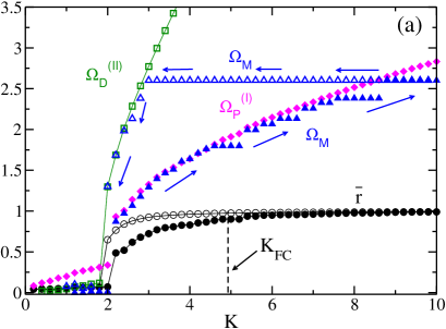
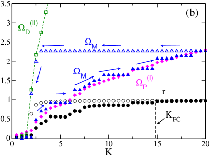
Figure 1: (Color Online) Average order parameter ${\bar{r}}$ (black circles) and maximal locking frequency $\Omega_{M}$ (blue triangles) as a function of the coupling $K$ for two series of simulations performed following the protocol (I) (filled symbols) and the protocol (II) (empty symbols). The data refer to mass: $m=2$ (a) and $m=6$ (b). For $m=2$ ($m=6$) we set $\Delta K=0.2$ ($\Delta K=0.5$) and $K_{M}=10$ ($K_{M}=20$), in both cases $N=500$, $T_{R}=5,000$ and $T_{W}=200$. The (magenta) diamonds indicate $\Omega_{P}^{(I)}=\frac{4}{\pi}\sqrt{\frac{K\bar{r}}{m}}$ for protocol (I), the (green) squares $\Omega_{D}^{(II)}=K\bar{r}$ for protocol (II), and the (black) dashed vertical line the coupling constant $K^{G}_{FC}$, whose expression is reported in Eq. (14).

An example of the outcome obtained by performing the sequence of simulations of protocol (I) followed by protocol (II) is reported in Fig. 1 for not negligible inertia, namely, $m=2$ and $m=6$. During the first series of simulations (I) the system remains desynchronized up to a threshold $K=K_{1}^{c}\simeq 2$, above this value $\bar{r}$ shows a jump to a finite value and then increases with $K$, saturating to $\bar{r}\simeq 1$ at sufficiently large coupling . By decresing $K$ one observes that the value of $\bar{r}$ assumes larger values than during protocol (I), while the system desynchronizes at a smaller coupling, namely $K_{2}^{c}<K_{1}^{c}$. Therefore, the limit of stability of the asynchronous state is given by $K_{1}^{c}$, while the partially synchronized state can exist down to $K_{2}^{c}$, thus asynchronous and partially synchronous states coexist in the interval $[K_{2}^{c};K_{1}^{c}]$.

The maximal locking frequency $\Omega_{M}$ increases with $K$ during the first phase. In particular, for sufficiently large coupling, $\Omega_{M}$ displays plateaus followed by jumps for large coupling: this indicates that the oscillators frequencies $\Omega_{i}$ are grouped in small clusters. Finally, for $\bar{r}\simeq 1$ the frequency $\Omega_{M}$ attains a maximal value. By reducing the coupling, following now the protocol (II), $\Omega_{M}$ remains stucked to such a value for a large $K$ interval. Then $\Omega_{M}$ reveals a rapid decrease towards zero for small coupling $K\simeq K_{2}^{c}$. In the next Section, we will give an interpretation of this behaviour.

We will also perform a series of simulations with a different protocol (S), to test for the independence of the results reported for $K_{1}^{c}$ and $K_{2}^{c}$ from the chosen initial conditions. In particular, for a certain coupling $K$ we consider an asynchronous initial condition and we perturb such a state by forcing all the neurons with natural frequency $|\Omega_{i}|<\omega_{S}$ to be locked. Namely, we initially set their velocities and phase to zero, then we let evolve the system for a transient time $T_{R}$ followed by a period $T_{W}$ during which ${\bar{r}}$ and the other quantities of interest are measured. These simulations will be employed to identify the interval of coupling parameters over which the coherent and incoherent solutions can be numerically observed.

In more details, to measure with this approach $K_{1}^{c}$, which represents the upper coupling value for which the incoherent state can be observed, we fix the coupling $K$ and we perform a series of simulations for increasing $\omega_{S}$ values, namely from $\omega_{S}=0$ to $\omega_{S}=3$ in steps $\Delta\omega_{S}=0.05$. For each simulation we measure the order parameter $\bar{r}$, whenever it is finite for some $\omega_{S}>0$, the corresponding coupling is associated to a partially synchronized state, the smallest coupling for which this occurs is identified as $K_{c}^{1}$.

In order to identify $K_{2}^{c}$, which is the lower value of the coupling for which the coherent state is numerically observable, we measure the minimal $K$ for which the unperturbed asynchronous state (corresponding to $\omega_{S}=0$) spontaneously evolves towards a partially synchronized solution. To give a statistically meaningfull estimation of $K_{c}^{1}$ and $K_{2}^{c}$, we have averaged the results obtained for various different initial conditions, ranging from 5 to 8, for all the considered system sizes and masses.

In principle, this approach cannot test rigorously for the stability of the coherent and incoherent states, since it deals with a very specific perturbation of the initial state. However, as we will show the estimations of the critical couplings obtained with protocol (S) coincide with those given by protocols (I) and (II), thus indicating that the reported results are not critically dependent on the chosen initial conditions.

Figure 2: (Color Online) Minimal $\omega_{S}$ giving rise to a state characterized by a finite level of synchronization (i.e. $\bar{r}>0$) as a function of the coupling constant $K$. The inset reports the minimal number $N_{S}$ of oscillators which should be initially locked in order to lead to the emergence of a coherent state, as a function of $K$. The vertical (green) dot-dashed line refers to the estimated $K_{1}^{c}$ and the (blue) dashed line indicates the estimated $K_{2}^{c}$. The data refer to simulations performed with protocol (S) for $N=16,000$, $m=6$, with $T_{W}=2,000$ and $T_{R}=20,000$.

III Mean Field Theory

In the fully coupled case Eq. (1) can be rewritten, by employing the order parameter definition (2) as follows

$$m\ddot{\theta}_{i}+\dot{\theta}_{i}=\Omega_{i}-Kr\sin(\theta_{i}-\phi)\qquad;$$ (3)

which corresponds to a damped driven pendulum equation. This equation admits for sufficiently small forcing frequency $\Omega_{i}$ two fixed points: a stable node and a saddle. At larger frequencies $\Omega_{i}>\Omega_{P}\simeq\frac{4}{\pi}\sqrt{\frac{Kr}{m}}$ a homoclinic bifurcation leads to the emergence of a limit cycle from the saddle. The stable limit cycle and the stable fixed point coexist until a saddle node bifurcation, taking place at $\Omega_{i}=\Omega_{D}=Kr$, leads to the disappearence of the fixed points and for $\Omega_{i}>\Omega_{D}$ only the oscillating solution is presents. This scenario is correct for sufficiently large masses, at small $m$ one have a direct transition from a stable node to a periodic oscillating orbit at $\Omega_{i}=\Omega_{D}=Kr$ Strogatz (2006).

Therefore for sufficiently large $m$ there is a coexistence regime where, depending on the initial conditions, the single oscillator can rotate or stay quiet. How this single unit property will reflect in the self-consistent collective dynamics of the coupled systems is the topic of this paper.

III.1 The Theory of Tanaka, Lichtenberg, and Oishi

Tanaka, Lichtenberg, and Oishi in their seminal papers Tanaka et al. (1997b, a) have examined the origin of the first order hysteretic transition observed for Lorentzian and flat (bounded) frequency distributions $g(\Omega)$ by considering two different initial states for the network : (I) the completely desynchronized state ($r=0$) and (II) the fully synchronized one ($r\equiv 1$). Furthermore, in case I (II) they studied how the level of synchronization, measured by $r$, varies due to the increase (decrease) of the coupling $K$. In the first case the oscillators are all initially drifting with finite velocities $\langle\dot{\theta}_{i}\rangle$; by increasing $K$ the oscillators with smaller natural frequencies $|\Omega_{i}|<\Omega_{P}$ begin to lock ($\langle\dot{\theta}_{i}\rangle=0$), while the other continue to drift. This picture is confirmed by the data reported in Fig. 1, where the maximal value $\Omega_{M}$ of the frequencies of the locked oscillators is well approximated by $\Omega_{P}$. The process continues until all the oscillators are finally locked leading to $r=1$.

In the case (II), TLO assumed that initially all the oscillators were already locked, with an associated order parameter $r\equiv 1$. Therefore, the oscillators can start to drift only when the stable fixed point solution will disappear, leaving the system only with the limit cycle solution. This happens, by decreasing $K$, whenever $|\Omega_{i}|\geq\Omega_{D}=Kr$. This is numerically verified, indeed, as shown in Fig. 1, the maximal locked frequency $\Omega_{M}$ remains constant until, by decreasing $K$, it encounters the curve $\Omega_{D}$ and then $\Omega_{M}$ follows this latter curve down to the desynchronized state. The case (II) corresponds to the situation observable for the usual Kuramoto model, where there is no bistability Kuramoto (2003).

In both the examined cases there is a group of desynchronized oscillators and one of locked oscillators separated by a frequency, $\Omega_{P}$ in the first case and $\Omega_{D}$ in the second one. These groups contribute differently to the total level of synchronization of the system, namely

$$r=r_{L}+r_{D}$$ (4)

where $r_{L}$ ($r_{D}$) is the contribution of the locked (drifting) population.

For the locked population, one gets

$$r_{L}^{I,II}=Kr\int_{-\theta_{P,D}}^{\theta_{P,D}}\cos^{2}\theta g(Kr\sin\theta)d\theta\qquad;$$ (5)

where $\theta_{P}=\sin^{-1}(\Omega_{P}/Kr)$ and $\theta_{D}=\sin^{-1}(\Omega_{D}/Kr)\equiv\pi/2$.

The drifting oscillators contribute to the total order parameter with a negative contribution; the self-consistent integral defining $r_{D}$ has been estimated by TLO in a perturbative manner by performing an expansion up to the fourth order in $1/(mK)$ and $1/(m\Omega)$. Therefore the obtained expression is correct in the limit of sufficiently large masses and it reads as

$$r_{D}^{I,II}\simeq-mKr\int_{\Omega_{P,D}}^{\infty}\frac{1}{(m\Omega)^{3}}g(\Omega)d\Omega\qquad;$$ (6)

where $g(\Omega)=g(-\Omega)$.

By considering an initially desynchronized (fully synchronized) system and by increasing (decreasing) $K$ one can get a theoretical approximation for the level of synchronization in the system by employing the mean-field expression (5), (6) and (4) for case I (II). In this way, two curves are obtained in the phase plane $(K,r)$, namely $r^{I}(K)$ and $r^{II}(K)$. In the following, we will show that these are not the unique admissible solutions in the mentioned plane, and these curves represent the lower and upper bound for the possible states characterized by a partial level of synchronization.

Let us notice that the expression for $r_{L}$ and $r_{D}$ reported in Eqs. (5) and (6) are the same for case (I) and (II), only the integration extrema have been changed. These are defined by the frequency which discriminates locked from drifting neuron, that in case (I) is $\Omega_{P}$ and in case (II) $\Omega_{D}$. The value of these frequencies is a function of the order parameter $r$ and of the coupling constant $K$, therefore by increasing (decreasing) $K$ they change accordingly.

However, in principle one could fix the discriminating frequency to some arbitrary value $\Omega_{0}$ and solve self-consistently the equations Eqs. (4), (5), and (6) for different values of the coupling $K$. This amounts to solve the following equation

$$\int_{-\theta_{0}}^{\theta_{0}}\cos^{2}\theta g(Kr^{0}\sin\theta)d\theta-m\int_{\Omega_{0}}^{\infty}\frac{1}{(m\Omega)^{3}}g(\Omega)d\Omega=\frac{1}{K}\qquad;$$ (7)

with $\theta_{0}=\sin^{-1}(\Omega_{0}/Kr^{0})$. Thus obtaining a solution $r^{0}=r^{0}(K,\Omega_{0})$, which exists provided that $\Omega_{0}\leq\Omega_{D}(K)=r^{0}K$. Therefore a portion of the $(K,r)$ plane, delimited by the curve $r^{II}(K)$, will be filled with the curves $r_{0}(K)$ obtained for different $\Omega_{0}$ values (as shown in Fig. 3 for fully coupled systems and in Fig. 14 for diluted ones.). These solutions represent clusters of $N_{L}$ oscillators for which the maximal locking frequency and $N_{L}$ do not vary upon changing the coupling strength. These states will be the subject of numerical investigation of the next Sections. In particular, we will show via numerical simulations that for $K>K_{2}^{c}$ these states are numerically observables within the portion of the phase space delimited by the two curves $r^{I}(K)$ and $r^{II}(K)$ (see Fig. 3 and Fig. 14).

III.2 Linear Stability Limit for the Incoherent Solution

As a final aspect, we will report the results of a recent theoretical mean field approach based on the Kramers description of the evolution of the single oscillator distributions for coupled oscillators with inertia and noise Acebrón et al. (2000); Gupta et al. (2014). In particular, the authors in Gupta et al. (2014) have derived an analytic expression for the coupling $K_{1}^{MF}$, which delimits the range of linear stability for the asynchronous state. In the limit of zero noise, $K_{1}^{MF}$ can be obtained by solving the following equation

$$\frac{1}{K_{1}^{MF}}=\frac{\pi g(0)}{2}-\frac{m}{2}\int_{-\infty}^{\infty}\frac{g(\Omega)d\Omega}{1+m^{2}\Omega^{2}}\qquad;$$ (8)

where $g(\Omega)$ is an unimodal distribution of width $\sigma$. In the limit $m\to 0$ one recovers the value of the critical coupling for the usual Kuramoto model Kuramoto (2003), namely $K_{1}^{MF}(m\equiv 0)=2/(\pi g(0))$. For a Lorentzian distribution an explicit espression for any value of the mass can be obtained

$$K_{1}^{MF}=2\sigma(1+m\sigma)\quad;$$ (9)

which coincides with the one reported by Acebrón et al Acebrón et al. (2000). For a Gaussian distribution it is not possible to find an explicit expression for any $m$, however one can derive the first corrective terms to the zero mass limit, namely

$$K_{1}^{MF}=2\sigma\sqrt{\frac{2}{\pi}}\left\{1+\sqrt{\frac{2}{\pi}}m\sigma+\frac{2}{\pi}m^{2}\sigma^{2}+\sqrt{\left(\frac{2}{\pi}\right)^{3}-\frac{2}{\pi}}m^{3}\sigma^{3}\right\}+{\cal O}(m^{4}\sigma^{4})\quad.$$ (10)

On the opposite limit one can analytically show that the critical coupling diverges as

$$K_{1}^{MF}\propto 2m\sigma^{2}\qquad{\rm for}\qquad m\sigma\to\infty\quad.$$ (11)

It can be seen that this scaling is already valid for not too large masses, indeed the analytical results obtained via Eq. (8) are very well approximated, in the range $m\in[1:30]$, by the following expression

$$K_{1}^{MF}\simeq 2\sigma(0.64+m\sigma)\quad.$$ (12)

This result, together with Eq. (9), indicates that for both the Lorentzian and the Gaussian distribution the critical coupling diverges linearly with the mass and quadratically with the width of the frequency distribution.

In the next Section we will compare our numerical results for various system sizes with the mean-field result (8).

III.3 Limit of Complete Synchronization

Complete synchronization can be achieved, in the ideal case of infinite oscillators with a distribution $g(\Omega)$ with infinite support, only in the limit of infinite coupling. However, in finite systems an (almost) complete synchronization is attainable already at finite coupling, to give an estimation of this effective coupling $K_{FC}$ one can proceed as follows. Let us estimate the pinning frequency ${\bar{\Omega}}_{P}$ required to have a large percentage of oscillators locked, this can be implicitely defined as, e.g.

$$\int_{-{\bar{\Omega}}_{P}}^{{\bar{\Omega}}_{P}}g(\Omega)d\Omega=0.954\qquad;$$ (13)

where by assuming $r\simeq 1$ one sets ${\bar{\Omega}}_{P}\simeq\frac{4}{\pi}\sqrt{\frac{K_{FC}}{m}}$ and from Eq. (13) one can derive the coupling $K_{FC}$. For a Gaussian distribution the integral reported in Eq. (13) amounts to consider two standard deviations, and therefore one gets

$$K_{FC}^{G}\simeq\left(\frac{\pi}{2}\right)^{2}m\sigma^{2}\qquad;$$ (14)

while for a Lorentzian distribution $g(\Omega)=\frac{\sigma}{\pi}\frac{1}{\sigma^{2}+\Omega^{2}}$ this corresponds to

$$K_{FC}^{L}\simeq\left(\frac{13.815\pi}{4}\right)^{2}m\sigma^{2}\qquad.$$ (15)

These results reveal that for increasing mass and width of the frequency distribution the system becomes harder and harder to fully synchronize and that to achieve the same level of synchronization a much larger coupling is required for the Lorentzian distribution (for the same $m$ and $\sigma$).

IV Fully Coupled System

In this Section we will compare the analytical results with finite $N$ simulations for the fully coupled system: a first comparison is reported in Fig. 3 for two different masses, namely $m=2$ and $m=6$. We observe that the data obtained by employing the procedure (II) are quite well reproduced from the mean field approximation $r^{II}$ for both masses (solid red curve in Fig. 3). This is not the case for the theoretical estimation $r^{I}$ (dashed red curve), which for $m=2$ is larger than the numerical data up to quite large coupling, namely $K\simeq 5$; while for $m=6$, a better agreement is observable at smaller $K$, however now $\bar{r}$ reveals a step-wise structure for the data corresponding to procol (I). This step-wise structure at large masses is due to the break down of the independence of the whirling oscillators: namely, to the formation of locked clusters at non zero velocities Tanaka et al. (1997a). Therefore, oscillators join in small groups to the locked solution and not individually as it happens for smaller masses; this is clearly revealed by the behaviour of $N_{L}$ versus the coupling $K$ as reported in the insets of Fig. 3(b).

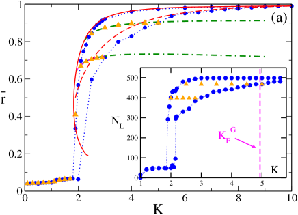
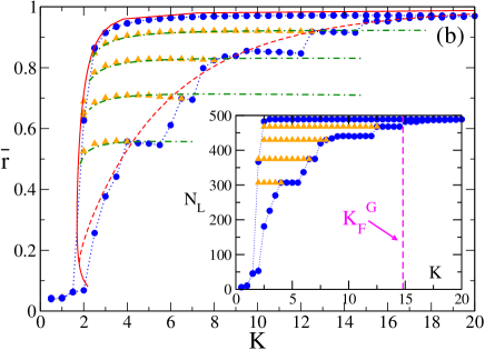
Figure 3: (Color Online) Average order parameter ${\bar{r}}$ versus the coupling constant $K$ for $m=2$ (a) and $m=6$ (b). Mean field estimates: the dashed (solid) red curves refer to $r^{I}=r^{I}_{L}+r^{I}_{D}$ ($r^{II}=r^{II}_{L}+r^{II}_{D}$) as obtained by employing Eqs. (5) and (6) following protocol (I) (protocol (II)); the (green) dot-dashed curves are the solutions $r^{0}(K,\Omega_{0})$ of Eq. (7) for different $\Omega_{0}$ values. The employed values from bottom to top are: $\Omega_{0}=1.21$ and 1.71 in (a) and $\Omega_{0}=0.79$, 1.09, 1.31, and 1.79 in (b).Numerical simulations: (blue) filled circles have been obtained by following protocol (I) and then (II) starting from $K=0$ until $K_{M}=10$ ($K_{M}=20$) for mass $m=2$ ($m=6$) with steps $\Delta K=0.2$ ($\Delta K=0.5$); (orange) filled triangles refer to simulations performed by starting from a final configuration obtained during protocol (I) and by decreasing the coupling from such initial configurations. The insets display $N_{L}$ vs $K$ for the numerical simulations reported in the main figures, the value of $K_{F}^{G}$ (eq.(14)) is also reported in the two cases. The numerical data refer to $N=500$, $T_{R}=5000$, and $T_{W}=200$.

IV.1 Hysteretic Behaviour

As already mentioned, we would like to better investigate the nature of the hysteresis observed by performing simulations accordingly to protocol (I) or protocol (II). In particular, we consider as initial condition a partially synchronized state obtained during protocol (I) for a certain coupling $K_{S}>K_{1}$, then we perform a sequence of consecutive simulations by reducing the coupling at regular steps $\Delta K$. Some example of the obtained results are shown in Fig. 3, where we report $\bar{r}$ and $N_{L}$ measured during such simulations as a function of the coupling (orange filled triangles). From the simulations it is evident that the number of locked oscillators $N_{L}$ remains constant until we do not reach the descending curve obtained with protocol (II). On the other hand $\bar{r}$ decreases slightly with $K$, this decrease can be well approximated by the mean field solutions of Eq. (7), namely $r^{0}(K,\Omega_{0})$ with $\Omega_{0}=\Omega_{P}(K_{s},r^{I}(K_{S}))=\frac{4}{\pi}\sqrt{\frac{K_{s}r^{I}}{m}}$, see the green dot-dashed lines in Fig. 3 for $m=2$ and $m=6$. However, as soon as, by decreasing $K$, the frequency $\Omega_{0}$ becomes equal or smaller than $\Omega_{D}$, the order parameter has a rapid drop towards zero following the upper limit curve $r^{II}$.

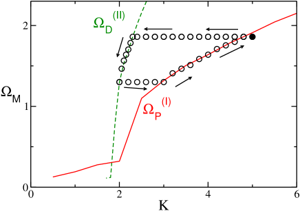
Figure 4: (Color Online) Maximal locking frequency $\Omega_{M}$ versus the coupling constant $K$. The initial state is denoted by the filled circle at $K_{I}=5$. The solid (red) curve indicates the frequency $\Omega_{P}^{(I)}$ and the dashed (green) curve the frequency $\Omega_{D}^{(II)}$. The numerical data refer to $N=500$, $T_{R}=5000$, $T_{W}=200$, $m=2$, and $\Delta K=0.1-0.05$.

To better interpret these results, let us focus on a simple numerical experiment. We consider a partially synchronized state obtained for $K_{I}=5$ with $N=500$ oscillators, then we first decrease the coupling in steps $\Delta K$ up to a coupling $K_{F}=2$ and then we increase again $K$ to return to the initial value $K_{I}$. During such cyclic simulation we measure $\Omega_{M}$ for each examined states, the results are reported in Fig. 4. It is clear that initially $\Omega_{M}$ does not vary and it remains identical to its initial value at $K_{I}=5$. Furthermore, also the number of locked oscillators $N_{L}$ remains constant. The maximal locking frequency (as well as $N_{L}$) starts to decrease with $K$ only after $\Omega_{M}$ has reached the curve $\Omega_{D}^{(II)}$, then it follows exactly this curve, corresponding to protocol (II), until $K=K_{F}$. At this point we increase again the coupling: the measured $\Omega_{M}$ stays constant at the value $\Omega_{D}^{(II)}=2*r^{II}(K_{F})$. The frequency $\Omega_{M}$ starts to increase only after its encounter with the curve $\Omega_{P}^{(I)}(K)$. In the final part of the simulation $\Omega_{M}$ recovers its initial value by following this latter curve. From these simulations it is clear that a synchronized cluster can be modified by varying the coupling, only by following protocol (I) or protocol (II), otherwise the coupling seems not to have any relevant effect on the cluster itself. In other words, all the states $(K,\Omega_{M})$ contained between the curves $\Omega_{D}^{(II)}$ and $\Omega_{P}^{(I)}$ are reachable for the system dynamics, however they are quite peculiar.

We have verified that the path connecting the initial state at $K_{I}$ to the curve $\Omega_{D}^{(II)}(K)$, as well as the one connecting $K_{F}$ to the curve $\Omega_{P}^{(I)}(K)$, are completely reversible. We can increase (decrease) the coupling from $K_{I}$ ($K_{F}$) up to any intermediate coupling value in steps of any size $\Delta K$ and then decrease (increase) the coupling to return to $K_{I}$ ($K_{F}$) by performing the same steps and the system will pass exactly from the same states, characterized for each examined $K$ by the values of $\bar{r}$ and $\Omega_{M}$. Furthermore, as mentioned, there is no dependence on the employed step $\Delta K$, apart the restriction that the reached states should be contained within the phase space portion delimited by the two curves $\Omega_{D}^{(II)}$ and $\Omega_{P}^{(I)}$. As soon as the coupling variations would eventually lead the system outside this portion of the phase space, one should follow a hysteretic loop to return to the initial state, similar to the one reported in Fig. 4. Therefore, we can affirm that hysteretic loop of any size are possible within this region of the phase space. For what concerns the stability of these states, we can only affirm that from a numerical point of view they appear to be stable within the considered integration times. However, a (linear) stability analysis of these solutions is required to confirm our numerical observations.

IV.2 Finite Size Effects

Let us now examine the influence of the system size on the studied transitions, in particular we will estimate the transition points $K_{1}^{c}$ ($K_{2}^{c}$) by considering either a sequence of simulations obtained accordingly to protocol (I) (protocol (II)) or asynchronous (synchronous) initial conditions and by averaging over different realizations of the distributions of the forcing frequencies $\{\Omega_{i}\}$.

The results for the protocol (I) , protocol (II) simulations are reported in Fig. 5 for sizes ranging from $N=500$ up to $N=16,000$. It is immediately evident that $K_{2}^{c}$ does not depend heavily on $N$, while the value of $K_{1}^{c}$ is strongly influenced by the size of the system. Starting from the asynchronous state the system synchronizes at larger and larger coupling $K_{1}^{c}$ with an associated jump in the order parameter which increases with $N$. Whenever the system starts to synchronize, then it follows reasonably well the mean field TLO prediction and this is particularly true on the way back towards the asynchronous state along the path associated to protocol (II) procedure. However, TLO theory largely fails in giving an estimation of $K_{1}^{c}$ for large system sizes, as shown in Fig. 5.

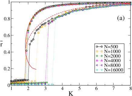
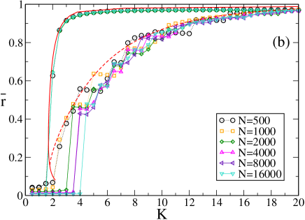
Figure 5: (Color Online) Average order parameter $\bar{r}$ versus the coupling constant $K$ for various system sizes $N$: (a) $m=2$ and (b) $m=6$. The (red) solid and dashed curves are the theoretical estimates already reported in Fig. 3. The numerical data have been obtained by following protocol (I) and then protocol (II) from $K=0$ up to $K_{M}=10$ ($K_{M}=20$) for mass $m=2$ ($m=6$) with $\Delta K=0.2$ ($\Delta K=0.5$). Data have been obtained by averaging the order parameter over a time window $T_{W}=200$, after discarding a transient time $T_{R}\simeq 1,000-80,000$ depending on the system size, the larger $T_{R}$ have been employed for the larger $N$.

In the following, we will analyze if the reported finite size results, and in particular the values of the critical couplings $K_{1}^{c}$ and $K_{2}^{c}$, depend on the initial conditions and on the simulation protocols. For this analysis we focus on two masses, namely $m=2$ and $m=6$, and we consider system sizes ranging from $N=500$ to $N=16,000$. For each size and mass we evaluate $K_{1}^{c}$ ($K_{2}^{c}$) by following protocol (I) (protocol (II)), as already shown in Fig. 5; furthermore now the critical coupling are also estimated by considering random initial conditions and by applying the protocol (S).

The results are reported in Fig. 6 for four different values of the mass; it is clear, by looking at the data displayed in Figs. 6(c) and (d), that protocol (I) (protocol (II)) and protocol (S) give essentially the same critical couplings, suggesting that their values are not dependent on the chosen initial conditions. Furthermore, while $K_{2}^{c}$ reveals a weak dependence on $N$, $K_{1}^{c}$ increases steadily with the system size. On the basis of our numerical data, it seems that the growth slow down at large $N$, but we are unable to judge if $K_{1}^{c}$ is already saturated to an asymptotic value at the maximal reached system size, namely $N=16,000$. To clarify this issue we compare our numerical results for $K_{1}^{c}$ with the mean field estimated $K_{1}^{MF}$ reported in Eq. (8). The mean field result is always larger than the finite size measurements, however for small masses, namely $m=0.8$ and $m=1.0$, $K_{1}^{c}$ seems to approach this asymptotic value already for the considered number of oscillators, as shown in Figs. 6(a) and (b). Therefore, in these two cases we attempt to identify the scaling law ruling the approach of $K_{1}^{c}$ to its mean field value for increasing system sizes. The results reported in Fig. 7 suggest the following power law

$$[K_{1}^{MF}-K_{1}^{c}(N)]\propto N^{-\gamma}\quad;$$ (16)

with $\gamma\simeq 0.22-0.23$.

Let us now consider several different values of the mass in the range $0.8\leq m\leq 30$; the data for the critical couplings are reported in Fig 8 for different system sizes ranging from $N=1,000$ to $N=16,000$. It is evident that $K_{1}^{c}$ grows with $N$ for all masses, while $K_{2}^{c}$ varies in a more limited manner. In particular, the estimated $K_{2}^{c}$ shows an initial decrease with $m$ followed by a constant plateau at larger masses (as shown in Fig 8 (b)). A possible mean field estimation for $K_{2}^{c}$ can be given by the minimal value $K^{II}_{m}$ reached by the coupling along the TLO curve $r^{II}(K)$. This value is reported in Fig 8 (b) together with the finite size data: at small masses $K^{II}_{m}$ gives a reasonable approximation of the numerical data, while at larger masses it is always smaller than the finite size results and it saturates to a constant value for $m\to\infty$. These results indicate that finite size fluctuations destabilizes the coherent state at larger coupling than those expected from a mean field theory.

On the other hand $K_{1}^{c}$ appears to increase with $m$ up to some maximal value and then to decrease at large masses. However, this is clearly a finite size effect, since by increasing $N$ the position of the maximum shifts to larger masses. The finite size curves $K_{1}^{c}=K_{1}^{c}(m,N)$ are always smaller than the mean field result $K_{1}^{MF}$ (dashed orange line in Fig 8 (a)) for all considered system sizes and masses. However, as shown in the inset of Fig 8 (a), such curves collapse one over the other if the variables are properly rescaled, suggesting the following functional dependence

$$\xi\equiv\frac{K_{1}^{MF}-K_{1}^{c}(m,N)}{K_{1}^{MF}}=G\left(\frac{m}{N^{\gamma}}\right)\quad;$$ (17)

where $\gamma=1/5$. This result is consistent with the values of the scaling exponent $\gamma$ found for fixed mass by fitting the data with the expression reported in Eq. (16). However, we are unable to provide any argument to justify such scaling and further analysis are required to intepret these results. A possible strategy could be to extend the approach reported in  Hong et al. (2007) for the finite size analysis of the usual Kuramoto transition to the Kuramoto model with inertia.

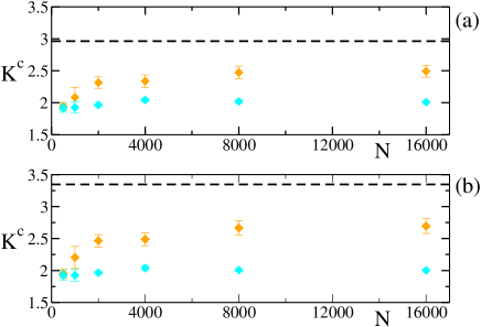
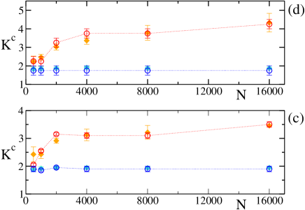
Figure 6: (Color Online) Critical couplings $K_{1}^{c}$ (orange filled diamonds and red empty circles) and $K_{2}^{c}$ (cyan filled diamonds and blue empty circles) versus the system size $N$: (a) $m=0.8$, (b) $m=1$, (c) $m=2$, and (d) $m=6$. The filled symbols refer to estimates performed with protocol (S), while empty symbols, in panels (c) and (d), have been obtained with protocol (I) (protocol (II)) for $K^{c}_{1}$ ($K_{2}^{c}$). The dashed (black) lines in panels (a) and (b) are the mean field values $K_{1}^{MF}$. This quantity is not reported in panels (c) and (d) for clarity reasons, due to its large value, namely, $K_{1}^{MF}=5.31$ for $m=2$ and $K_{1}^{MF}=13.27$ for $m=6$. For all panels the data have been derived by averaging in time over a window $T_{W}=2,000$ and over 8 (5) different initial conditions for the protocol (S) (protocol (I) and (II)). For each simulation an initial a transient time $T_{R}\simeq 20,000$ ($T_{R}\simeq 1,000-80,000$) has been discarded for protocol (S) (protocol (I) and (II)).

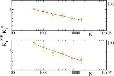
Figure 7: (Color Online) The differences $K_{1}^{MF}-K_{1}^{c}(N)$ (filled orange diamonds) are reported versus the system size $N$ for (a) $m=0.8$ and (b) $m=1$. The dashed (black) lines in both panels are power-law fits to the data: the difference vanishes as $0.42\times N^{-0.23}$ for $m=0.8$ (a) and as $5.27\times N^{-0.22}$. for $m=1$ (b). The data for $K_{1}^{c}$ are the same reported in panel (a) and (b) in Fig. 6.

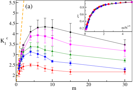
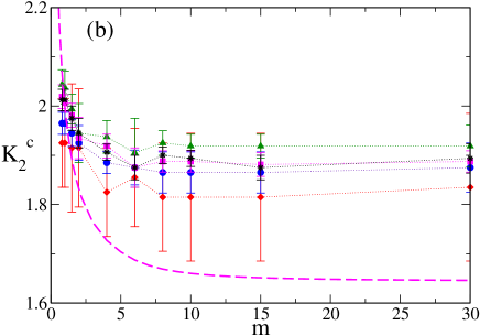
Figure 8: (Color Online) Critical couplings $K_{1}^{c}$ (a) and $K_{2}^{c}$ (b) versus the mass $m$ for different system sizes $N$. Namely, $N=1,000$ (red diamond), 2,000 (blue circles), 4,000 (green triangles), 8,000 (magenta squares) and 16,000 (black asteriskes). The dashed (orange) line in (a) is the mean field estimates $K_{1}^{MF}$; while the dashed (magenta) line in (b) is the value $K^{II}_{m}$ obtained by the TLO theory. The inset in panel (a) report the critical rescaled couplings $\xi=(K_{1}^{MF}-K_{1}^{c})/K_{1}^{MF}$ as a function of $m/N^{1/5}$. The estimates have been obtained with protocol (S), by averaging in time over a window $T_{W}=2,000-4,000$ and over 8 different initial conditions. For each simulation an initial transient time $T_{R}\simeq 20,000$ has been discarded.

IV.3 Drifting Clusters

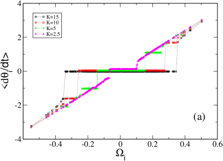
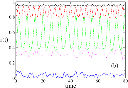
Figure 9: (Color Online) (a) Average phase velocity $\langle\dot{\theta}_{i}\rangle$ of the oscillators versus their natural frequencies $\Omega_{i}$: (magenta) triangles refer to $K=2.5$, (green) diamond to $K=5$, (red) squares to $K=10$ and (black) circles to $K=15$. For each simulation an initial transient $T_{R}\simeq 5,500$ has been discarded and the estimates have been obtained with protocol (I), by averaging in time over a window $T_{W}=5,000$. (b) Order parameter $r(t)$ versus time for $m=6$ and $N=500$ and different coupling constants $K$: the (blue) solid curve corresponds to $K=1$; the (magenta) dot-dashed line to $K=2.5$, the (green) dashed line to $K=5$, the (red) dashed line to $K=10$ and the (black) solid line to $K=15$. The data have been obtained by employing protocol (I) and for each simulation an initial transient time $T_{R}\simeq 1,500$ has been discarded and data are averaged over a time $T_{W}=5000$.

As already noticed in Tanaka et al. (1997a), for sufficiently large value of the mass one observes that the partially synchronized phase, obtained by following protocol (I), is characterized not only by the presence of the cluster of locked oscillators with $\langle\dot{\theta}\rangle\simeq 0$, but also by the emergence of clusters composed by drifting oscillators with finite average velocities. This is particularly clear in Fig. 9 (a), where we report the data for mass $m=6$. By increasing the coupling $K$ one observes for $K>3$ the emergence of a cluster of whirling oscillators with a finite velocity $|\langle\dot{\theta}\rangle|\simeq 1.05$, these oscillators have natural frequencies in the range $|\Omega_{i}|\simeq 0.15-0.25$. The number of oscillators in this secondary cluster $N_{DC}$ increases up to $K\simeq 5$, then it declines, finally the cluster is absorbed in the main locked group for $K\simeq 7$. At the same time a second smaller cluster emerges characterized by a larger average velocity $|\langle\dot{\theta}\rangle|\simeq 1.6$ (corresponding to larger $|\Omega_{i}|\simeq 0.27-0.34$). This second cluster merges with the locked oscillators for $K\simeq 12.5$, while a third one, composed of oscillators with even larger frequencies $|\Omega_{i}|$ and characterized by larger average phase velocity, arises. This process repeats until the full synchronization of the system is achieved.

The effect of these extra clusters on the collective dynamics is to induce oscillations in the temporal evolution of the order parameter, as one can see from Fig.  9 (b). In presence of drifting clusters characterized by the same average velocity (in absolute value), as for $m=6$ and $K=5$ in Fig.  9 (b), $r$ exhibits almost regular oscillations and the period of these oscillations is related to the one associated to the oscillators in the whirling cluster. This can be appreciated from Fig.  10 (b), where we compare the evolution of the istantaneuous velocity $\dot{\theta}_{i}$ for three oscillators and the time course of $r(t)$. We consider one oscillator $O_{1}$ in the locked cluster, and 2 oscillator $O_{2}$ and $O_{3}$ in the drifting cluster. We observe that these latter oscillators display essentially synchronized motions, while the phase velocity of $O_{1}$ oscillates irregularly around zero. Furthermore, the almost periodic oscillations of the order parameter $r(t)$ are clearly driven by the periodic oscillations of $O_{2}$ and $O_{3}$ (see Fig.  10 (b)).

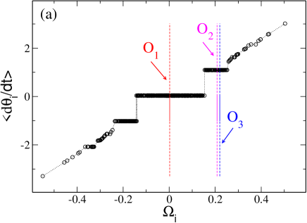
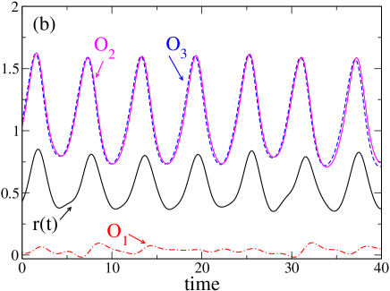
Figure 10: (Color Online) (a) Average phase velocity $\langle\dot{\theta}_{i}\rangle$ of the oscillators versus the corresponding natural frequency $\Omega_{i}$. The vertical dashed lines denote the three oscillators, $O_{1}$, $O_{2}$ and $O_{3}$, whose dynamical evolution is shown in (b). (b) The black curve represents the order parameter ${r}$ versus time, the other curves refer to the time evolution of the phase velocities $\dot{\theta}(t)$ of the three oscillators $O_{1}$ (red dot-dashed curve), $O_{2}$ (magenta solid line) and $O_{3}$ (dashed blue curve). For each simulation an initial transient time $T_{R}\simeq 1,000$ has been discarded, the averages reported in (a) have been obtained over a time window $T_{W}=20,000$. In both panels $K=5$, $m=6$ and $N=500$.

We have also verified that the amplitude of the oscillations of $r(t)$ (measured as the difference between the maximal $r_{max}$ and the minimal $r_{min}$ value of the order parameter) and the number of oscillators in the drifting clusters $N_{DC}$ correlates in an almost linear manner, as shown in Fig. 11 (b). Therefore we can conclude that the oscillations observable in the order parameter are induced by the presence of large secondary clusters characterized by finite whirling velocities. At smaller masses (e.g. $m=2$) oscillations in the order parameter are present, but they are much more smaller and irregular (data not shown). These oscillations are probably due to finite size effects, since in this case we do not observe any cluster of drifting oscillators in the whole range from asynchronous to fully synchronized state.

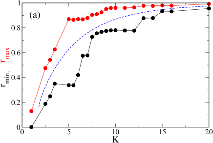
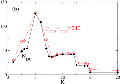
Figure 11: (Color Online) (a) Minima and maxima of the order parameter $r$ as a function of the coupling constant $K$. The (blue) dashed line refer to the theoretical estimate $r^{I}$, as obtained by employing Eqs. (5) and (6). (b) The number of oscillators in the drifting clusters $N_{DC}$ (filled black diamond) is reported versus the coupling $K$ together with the amplitude of the oscillations of the order parameter $r_{max}-r_{min}$ (empty red circles) rescaled by a factor 240. For each simulation an initial transient time $T_{R}\simeq 1,500$ has been discarded. The estimates have been obtained with protocol (I), by averaging in time over a window $T_{W}=5000$, $m=6$, $N=500$.

The situation was quite different in the study reported in Tanaka et al. (1997b), where the authors considered natural frequencies $\{\Omega_{i}\}$ uniformly distributed over a finite interval and not Gaussian distributed as in the present study. In that case, by considering an initially clusterized state, similar to what done for protocol (S), $r(t)$ revealed regular oscillations even for masses as small as $m=0.85$. In agreement with our results, the amplitude of the oscillations measured in Tanaka et al. (1997b) decreases by approaching the fully synchronized state (as shown in Fig.11). However, the authors in Tanaka et al. (1997b) did not relate the observed oscillations in $r(t)$ with the formation of drifting clusters.

As a final aspect, as one can appreciate from Fig. 5, for larger masses the discrepancies between the measured $\bar{r}$, obtained by employing protocol (I), and the theoretical mean field result $r^{I}$ increase. In order to better investigate the origin of these discrepancies, we report in Fig.11 the minimal and maximal value of $r$ as a function of the coupling $K$ and we compare these values to the estimated mean field value $r^{I}$. The comparison clearly reveals that $r^{I}$ is always contained between $r_{min}$ and $r_{max}$, therefore the mean field theory captures correctly the average increase of the order parameter, but it is unable to foresee the oscillations in $r$. A new version of the theory developed by TLO in Tanaka et al. (1997a) is required in order to include also the effect of clusters of whirling oscillators. A similar synchronization scenario, where oscillations in $r(t)$ are induced by the coexistence of several drifting clusters, has been recently reported for the Kuramoto model with degree assortativity Restrepo and Ott (2014).

V Diluted networks

In this Section we will analyze diluted neural networks obtained by considering random realizations of the coupling matrix $C_{i,j}$ with the constraints that the matrix should remain symmetric and the in-degree should be constant and equal to $N_{c}$ . In particular, we will examine if the introduction of the random dilution in the network will alter the results obtained by the mean-field theory and if the transition will remains hysteretic or not. For this analysis we limit ourselves to a single value of the mass, namely $m=2$.

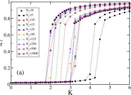
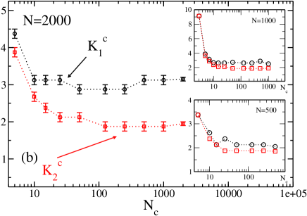
Figure 12: (Color Online) (a) Average order parameter ${\bar{r}}$ versus the coupling constant $K$ for diluted neural networks for various $N_{c}$: $5$ (filled black circlesa); 10 (red squares); 15 (green diamond); 25 (blue up triangles); 50 (orange left triangles); 125 (turquoise down triangles); 250 (right magenta triangles); 500 (violet crosses); 1,000 (empty maroon circles); 2,000 (black asteriskes). (b) Critical constants $K_{1}^{c}$ and $K_{2}^{c}$ estimated for various values of the in-degree. The numerical data refer to $N=2,000$; the upper inset refer to $N=1,000$, the lower one to $N=500$. For all simulations $m=2$, $T_{R}=10,000$, and $T_{W}=2,000$; each series of simulations have been obtained by following protocol (I) and then (II) starting from $K=0$ until $K_{M}=20$ with steps $\Delta K=0.25$. The reported data have been obtained by averaging over 10 - 20 different series of simulations, each corresponding to a different realization of the random network and of the distribution of the frequencies $\{\Omega_{i}\}$. The error bars in panel (b) correspond to $\Delta K/2$.

Let us first consider how the dependence of the order parameter $\bar{r}$ on the coupling constant $K$ will be modified in the diluted systems. In particular, we examine the outcomes of simulations performed with protocol (I) and (II) for a system size $N=2,000$ and different realizations of the diluted network ranging from the fully coupled case to $N_{c}=5$. The results, reported in Fig. 12, reveal that as far $N\geq 125$ (corresponding to the $\simeq 94\%$ of cutted links) it is difficult to distinguish among the fully coupled situation and the diluted ones. The small observed discrepancies can be due to finite size fluctuations. For larger dilution, the curves obtained with protocol (II) reveal a more rapid decay at larger coupling. Therefore $K_{2}^{c}$ increases by decreasing $N_{c}$ and approaches $K_{1}^{c}$ as shown in Fig. 12 (b). The dilution has almost no effect on the curve obtained with protocol (I), in particular $K_{1}^{c}$ remains unchanged (apart fluctuations within the error bars) until the percentage of incoming links $N_{c}/N$ reduces below the $0.5\%$. For smaller connectivities both $K_{1}^{c}$ and $K_{2}^{c}$ shift to larger coupling and they approach one another, indicating that the synchronization transition from hysteretic tends to become continuous. Indeed this happens for $N=1,000$ and $N=500$ (as shown in the inset of Fig. 12 (b)): for such system sizes we observe essentially the same scenario as for $N=2,000$, but already for in-degrees $N_{c}\leq 5$ the transition is no more hysteretic. This seems to suggest that by increasing the system size the transition will stay hysteretic for vanishingly small percentages of connected (incoming) links. This is confirmed by the data shown in Fig. 13, where we report the width of the hysteretic loop $W_{h}$, measured at a fixed value of the order parameter, namely we considered $\bar{r}=0.9$. For increasing system sizes $W_{h}$, measured for the same fraction of connected links $N_{c}/N$, increases, while the continuous transition, corresponding to $W_{h}\equiv 0$, is eventually reached for smaller and smaller value of $N_{c}/N$. Unfortunately, due to the CPU costs, we are unable to investigate in details diluted systems larger than $N=2,000$.

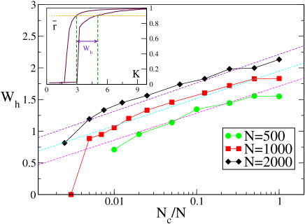
Figure 13: (Color Online) Width of the hysteretic loop $W_{h}$, measured in correspondence of a order parameter value $\bar{r}=0.9$, as a function of the percentage of connected links $N_{c}/N$. The (green) circles refer to $N=500$, the (red) squares to $N=1000$ and the (black) diamond to $N=2,000$. The dashed lines refer to logarithmic fitting to the data in the range $0.01<N_{c}/N\leq 1$. In the inset is graphically explained how $W_{h}$ has been estimated, starting from one of the curves reported in Fig. 12 (a). The data refer to the same parameters and simulation protocols as in Fig. 12.

Therefore, from this first analysis it emerges that the diluted or fully coupled systems, whenever the coupling is properly rescaled with the in-degree, as in Eq. 1, display the same phase diagram in the $(\bar{r},K)$-plane even for very large dilution. In the following we will examine if the mean-field results obtained by following the TLO approach still apply to the diluted system. The comparison reported in figure Fig. 14 confirms the good agreement between the numerical results obtained for a quite diluted system (namely, with 70 % of broken links) and the mean-field predictions (5) and (6). Furthermore, the data reported in Fig. 14 show that also in the diluted case all the states between the synchronization curves obtained following protocol (I) and protocol (II) are reachable and numerically stable, analogously to what shown in Subsect IV A for the fully coupled system. These states, displayed as orange filled triangles in Fig. 14, are characterized by a cluster composed by a constant number $N_{L}$ of locked oscillators with frequencies smaller than a value $\Omega_{M}$. The number of oscillators in the cluster $N_{L}$ remains constant by varying the coupling between the two synchronization curves (I) and (II). Finally, the generalized mean-field solution $r^{0}(K,\Omega_{0})$ (see Eq. (7)) is able, also in the diluted case, to well reproduce the numerically obtained paths connecting the synchronization curves (I) and (II) (see Fig. 14 and the inset).

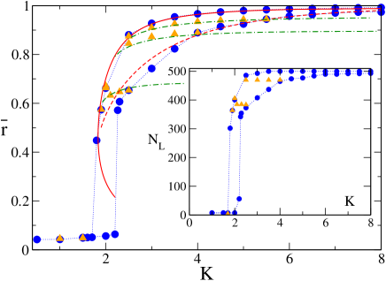
Figure 14: (Color Online) Average order parameter ${\bar{r}}$ versus the coupling constant $K$ for a diluted network with 70% of cutted links. Mean field estimates: the dashed (solid) red curves refer to $r^{I}=r^{I}_{L}+r^{I}_{D}$ ($r^{II}=r^{II}_{L}+r^{II}_{D}$) as obtained by employing Eqs. (5) and (6) following protocol I (protocol (II)); the (green) dot-dashed curves are the solutions $r^{0}(K,\Omega_{0})$ of Eq. (7) for different $\Omega_{0}$ values. The employed values from bottom to top are: $\Omega_{0}=2.05$, 1.69 and 1.10. Numerical simulations: (blue) filled circles have been obtained by following protocol (I) and then (II) starting from $K=0$ until $K_{M}=20$ with steps $\Delta K=0.5$; (orange) filled triangles refer to simulations performed by starting from a final configuration obtained during protocol (I) and by decreasing the coupling from such initial configurations. The insets display $N_{L}$ vs $K$ for the numerical simulations reported in the main figures. The numerical data refer to $m=2$, $N=500$, $N_{c}=150$, $T_{R}=5000$, and $T_{W}=200$.

VI A realistic network: the italian high-voltage power grid

In this Section, we examine if the previously reported features of the synchronization transition persist in a somehow more realistic setup. As we mentioned in the introduction a highly simplified model for a power grid composed of generators and consumers, resembling a Kuramoto model with inertia, can be obtained whenever the generator dynamics can be expressed in terms of the so-called swing equation Salam et al. (1984); Filatrella et al. (2008). The self-synchronization emerging in this model has been recently object of investigation for different network topologies Rohden et al. (2012); Fortuna et al. (2012); Rohden et al. (2014). In this paper we will concentrate on the Italian high-voltage (380 kV) power grid (Sardinia excluded), which is composed of $N=127$ nodes, divided in 34 sources (hydroelectric and thermal power plants) and 93 consumers, connected by 342 links Fortuna et al. (2012). This network is characterized by a quite low average connectivity $\langle N_{c}\rangle=2.865$, due to the geographical distributions of the nodes along Italy map .

In this extremely simplified picture, each node can be described by its phase $\phi_{i}(t)=\omega_{\rm AC}t+\theta_{i}(t)$, where $\omega_{\rm AC}=2\pi\times 50$ Hz or $2\pi\times 60$ Hz is the standard AC frequency and $\theta_{i}$ represents the phase deviation of the node $i$ from the uniform rotation at frequency $\omega_{\rm AC}$. Furthermore, the equation of motion for each node is assumed to be the same for consumers and generators; these are distiguished by the sign of a quantity $P_{i}$ associated each node: a positive (negative) $P_{i}$ corresponds to generated (consumed) power. By employing the conservation of energy and by assuming that the grid operates in proximity of the AC frequency (i.e. $|\dot{\theta}|<<\omega_{\rm AC}$) and that the rate at which the energy is stored (in the kinetic term) is much smaller than the rate at which is dissipated, the evolution equations for the phase deviations take the following expression Filatrella et al. (2008),

$$\ddot{\theta}_{i}=\alpha\left[-\dot{\theta}_{i}+P_{i}+K\sum_{j}C_{i,j}\sin(\theta_{j}-\theta_{i})\right]\qquad.$$ (18)

To maintain a parallel with the previously studied model (1), we have multiplied the left-hand side by a term $\alpha$, which in (18) represents the dissipations in the grid, while in (1) corresponds to the inverse of the mass. The parameter $\alpha\times K$ now represents the maximal power which can be transmitted between two connected nodes. More details on the model are reported in Salam et al. (1984); Filatrella et al. (2008); Rohden et al. (2014). It is important to stress that in order to have a stable, fully locked state, as possible solution of (18), it is necessary that the sum of the generated power equal the sum of the consumed power. Thus, by assuming that all the generators are identical as well as all the consumers, the distribution of the $P_{i}$ is made of two $\delta$-function located at $P_{i}=-C$ and $P_{i}=+G$. In our simulations we have set $C=1.0$, $G=2.7353$ and $\alpha=1/6$. This set-up corresponds to a Kuramoto model with inertia with a bimodal distribution of the frequencies.

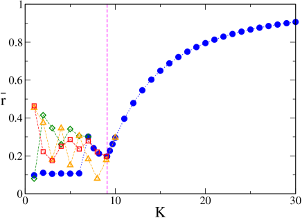
Figure 15: (Color Online) Average order parameter $\bar{r}$ versus the parameter $K$ for the Italian high-voltage power grid network. The (blue) circles data have been obtained by following protocol (I) from $K=1$ up to $K_{M}=40$ with $\Delta K=1$. The other symbols refer to simulations performed following protocol (II) starting from different intial coupling $K_{I}$ down to $K=1$, namely (orange) triangles $K_{I}=10$, (red) squares $K_{I}=9$ and (green) diamond $K_{I}=7$. The dashed vertical (magenta) line idicates the value $K=9$. The reported data have been obtained by averaging the order parameter over a time window $T_{W}=5,000$, after discarding an initial transient time $T_{R}\simeq 60,000$. The numerical data refer to $\alpha=1/6$, N=127, $<N_{c}>=2.865$.

As a first analysis we have performed simulations with protocol (I) for the model (18) by varying the parameter $K$ and we have measured the corresponding average order parameter $\bar{r}$. As shown in Fig. 15 the behaviour of $\bar{r}$ with $K$ is non-monotonic. For small $K$ the state is asynchronous with $\bar{r}\simeq 1/\sqrt{N}$, then $\bar{r}$ shows an abrupt jump for $K\simeq 7$ to a finite value, then it decreases reaching a minimum at $K\simeq 9$. For larger $K$ the order parameter increases steadily with $K$ tending towards the fully synchronized regime.

Figure 16: (Color Online) Average phase velocity of each oscillator $\langle\dot{\theta}_{i}\rangle$ versus the oscillator index for different values of the coupling $K$. The oscillators have been reordered so that the first 93 are consumers and the last 34 sources. The data have been obtained by employing protocol (I), starting from zero coupling $K=0$ and with $\Delta K=1$. For each simulation an initial transient time $T_{R}\simeq 5,000$ has been discarded and the average is taken over a window $T_{W}=5,000$. The numerical data refer to the same parameters as in Fig. 15.

This behaviour can be understood by examining the average phase velocity of the oscillators $\langle\dot{\theta}_{i}\rangle$. As shown in Fig. 16, for coupling $K<7$ the system is splitted in 2 clusters: one composed by the sources which oscillates with their proper frequency $G$ and the other one containing the consumers, which rotates with average velocity $-C$. The oscillators in the two clusters rotate indipendently one from the other, therefore $\bar{r}\simeq 1/\sqrt{N}$. For $K\simeq 7$ the oscillators get entrained (as shown in Fig. 16) and most of them are locked with almost zero average velocity, however a large part (50 over 127) form a secondary cluster of whirling oscillators with a velocity $\langle\dot{\theta}\rangle\simeq-0.127$. This secondary cluster has a geographical origin, since it includes power stations and consumers located in the central part and south part of Italy, Sicily included. The presence of this whirling cluster induces large oscillations in the order parameter (see Fig. 18 (a)), reflecting almost regular transitions from a desynchronized to a partially synchronized state. By increasing the coupling to $K=8$ the two clusters merge in an unique cluster with few scattered oscillators, however the average velocity is small but not zero, namely $\langle\dot{\theta}\rangle\simeq-0.05$ (as reported in Fig. 16). Therefore the average value of the order parameter $\bar{r}$ decreases with respect to $K=7$, where a large part of the oscillators was exactly locked. Up to $K=9$, the really last node of the network, corresponding to one generator in Sicily connected with only one link to the rest of the Italian grid, still continues to oscillate indipendently from the other nodes, as shown in Fig. 16. Above $K=9$ all the oscillators are finally locked in an unique cluster and the increase in the coupling is reflected in a monotounous increase in $\bar{r}$, similar to the one observed in standard Kuramoto models (see Fig. 15).

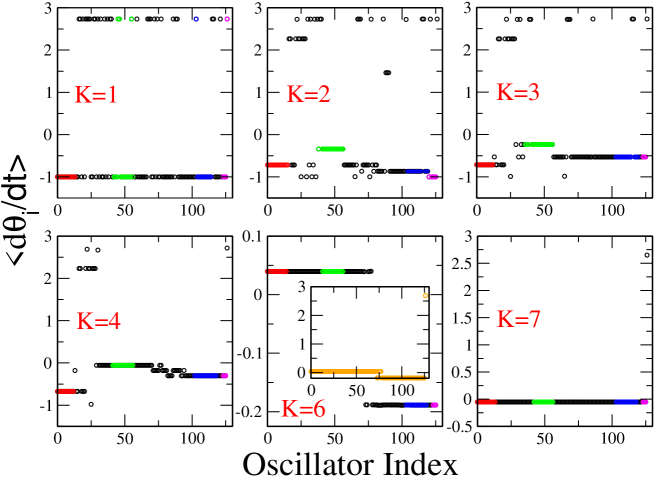
Figure 17: (Color Online) Average phase velocity of each oscillator $\langle\dot{\theta}_{i}\rangle$ versus the corresponding oscillator index, ordered following the geographical distribution from north Italy to Sicily. The panels refer to different couplings. The colored clusters indicate Italian regions which remains connected for all the considered simulations: red symbols refer to Piedmont and Liguria; green symbols to Veneto and Friuli Venetia Giulia; blue symbols to Campania and Apulia; magenta symbols to Sicily. The data have been obtained by employing protocol (II) starting from $K_{I}=12$ with $\Delta K=1$ down to $K=1$. For each simulation an initial transient time $T_{R}\simeq 50,000$ has been discarded and the averages performed over a window $T_{W}=5000$. The numerical data refer to the same parameters as in Fig. 15.

By applying protocol (II) we do not observe any hysteretic behaviour or multistability down to $K=9$; instead for smaller coupling a quite intricated behaviour is observable. As shown in Fig. 17 starting from $K_{I}=12$ and decreasing the coupling in steps of amplitude $\Delta K=1$, the system stays mainly in one single cluster up to $K=7$, apart the last node of the network which already detached from the network at some larger $K$. Indeed at $K=7$ the order parameter has a constant value around 0.2 and no oscillations. As shown in Fig.18 (b), by decreasing the coupling to $K=6$, wide oscillations emerge in $r(t)$ due to the fact that the locked cluster has splitted in two clusters, the separation is similar to the one reported for $K=7$ in Fig. 16. By further lowering $K$, several small whirling clusters appear and the behaviour of $r(t)$ becomes seemingly irregular for $2\leq K\leq 5$ as reported in Fig.18 (b). An accurate analysis of the dynamics in terms of the maximal Lyapunov exponent has revealed that the irregular oscillations in $r(t)$ reflect quasi-periodic motions, since the measured maximal Lyapunov is always zero for the whole range of the considered couplings. The presence of the inertial term, together with an architecture which favours a splitting based on the proximity of the oscillators, lead to the formation of several whirling clusters characterized by different average phase velocities. The value of the order parameter arises as a combination of these different contributions, each corresponding to a different oscillatory frequency. The splitting in different clusters is probably also at the origin of the multistability observed for $K<7$: depending on the past history the grid splits in clusters formed by different groups of oscillators and this gives rise to different average values of the order parameter (see Fig. 15).

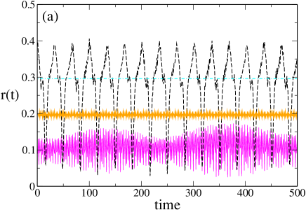
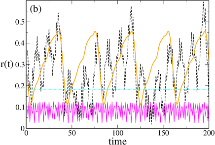
Figure 18: (Color Online) Order parameter $r(t)$ versus time for the Italian high-voltage power grid network for different values of the parameter $K$.Panel (a): the dotted (magenta) curve corresponds to K=4; the dashed (black) line to K=7; the solid (orange) line to K=9; the dot-dashed (cyan) line to K=10. The data have been obtained by employing protocol (I) and for each simulation an initial transient time $T_{R}\simeq 5,000$ has been discarded. Panel (b): the solid (magenta) curve corresponds to K=1; the dashed (black) line to K=4; the solid (orange) thick line to K=6; the dot-dashed (cyan) line to K=7. The data have been obtained by employing protocol (II) and for each simulation an initial transient time $T_{R}\simeq 50,000$ has been discarded. The simulations refer to the same parameters employed in Fig. 15.

We have verified that the emergence of several whirling clusters, with an associated quasi-periodic behaviour of the order parameter, is observable also by considering an unimodal (Gaussian) distribution of the $P_{i}$. This confirms that the main ingredients at the origin of this phenomenon are the inertial term together with a short-range connectivity. Thus the bimodal distribution, here employed, seems not to be crucial and it can only lead to an enhancement of such effect.

VII Conclusions

We have studied the synchronization transition for a globally coupled Kuramoto model with inertia for different system sizes and inertia values. The transition from incoherent to coherent state is hysteretic for sufficiently large masses. In particular, the upper value of the coupling constant ($K_{1}^{c}$), for which an incoherent state is observable, increases with the system sizes for all the examined masses. The estimated finite size value $K_{1}^{c}$ has a non monotonic dependence on the mass $m$, exhibiting a maximum at some intermediate value of $m$. However, all the data obtained for different masses and sizes collapse onto an universal curve, whenever the distance of $K_{1}^{c}$ with respect to its mean field value Gupta et al. (2014) is reported as a function of the mass divided by $N^{1/5}$. On the other hand, the coherent phase is attainable above a minimal critical coupling ($K_{2}^{c}$) which exhibits a weak dependence on the system size and it saturates to a constant asymptotic value for sufficiently large inertia values.

Furthermore, we have shown that clusters of locked oscillators of any size coexist within the hysteretic region. This region is delimited by two curves in the plane individuared by the coupling and the average value of the order parameter. Each curve corresponds to the synchronization (desynchronization) profile obtained starting from the fully desynchronized (synchronized) state. The original mean field theory developed by Tanaka, Lichtenberg, and Oishi in 1997 Tanaka et al. (1997a, b) gives a reasonable estimate of both these limiting curves, while a generalization of such theory is capable to reproduce all the possible synchronization/desynchronization hysteretic loops. However, the TLO theory does not take into account the presence of clusters composed by drifting oscillators emerging for sufficiently large masses. The coexistence of these clusters with the cluster of locked oscillator induces oscillatory behaviour in the order parameter.

The properties of the hysteretic transition have been examined also for random diluted network; the main properties of the transition are not affected by the dilution up to extremely high values. The transition appears to become continuous only when the number of links per node becomes of the order of few units. By increasing the system size the transition to the continuous case (if any) shifts to smaller and smaller values of the connectivity.

In this paper we focused on Gaussian distribution of the natural frequencies, however we have obtained similar results also for Lorentzian distributions. It would be however interesting to examine how the transition modifies in presence of non-unimodal distributions for the natural frequencies, like bimodal ones. Preliminary indications in this direction can be obtained by the reported analysis of the self-synchronization process occurring in the Italian high-voltage power grid, when the generators and consumers are mimicked in terms of a Kuramoto model with inertia Filatrella et al. (2008). In this case the transition is largely non hysteretic, probably this is due to the low value of the average connectivity in such a network. Coexistence of different states made of whirling and locked clusters, formed on regional basis, is observable only for electrical lines with a low value of the maximal transmissible power. These states are characterized by quasi-periodic oscillations in the order parameter due to the coexistence of several clusters of drifting oscillators.

A natural prosecution of the presented analysis would be the study of the stability of the observed clusters of locked and/or whirling oscillators in presence of noise. In this respect, exact mean-field results have been reported recently for fully coupled phase rotors with inertia and additive noise Gupta et al. (2014); Komarov et al. (2014). However, the emergence of clusters in such systems has been not yet addressed neither on a theoretical basis nor via direct simulations.