On linear convergence of a distributed dual gradient algorithm for linearly constrained separable convex problems

Abstract

In this paper we propose a distributed dual gradient algorithm for minimizing linearly constrained separable convex problems and analyze its rate of convergence. In particular, we prove that under the assumption of strong convexity and Lipshitz continuity of the gradient of the primal objective function we have a global error bound type property for the dual problem. Using this error bound property we devise a fully distributed dual gradient scheme, i.e. a gradient scheme based on a weighted step size, for which we derive global linear rate of convergence for both dual and primal suboptimality and for primal feasibility violation. Many real applications, e.g. distributed model predictive control, network utility maximization or optimal power flow, can be posed as linearly constrained separable convex problems for which dual gradient type methods from literature have sublinear convergence rate. In the present paper we prove for the first time that in fact we can achieve linear convergence rate for such algorithms when they are used for solving these applications. Numerical simulations are also provided to confirm our theory.

1 Introduction

Nowadays, many engineering applications which appear in the context of communications networks or networked systems can be posed as large scale linearly constrained separable convex problems. Several important applications that can be modeled in this framework, distributed model predictive control (DMPC) problem for networked systems [16], the network utility maximization (NUM) problem [2], and the direct current optimal power flow (DC-OPF) problem for a power system [1], have attracted great attention lately. Due to the large dimension and the separable structure of these problems, distributed optimization methods have become an appropriate tool for solving them.

Distributed optimization methods are based on decomposition [16]. Decomposition methods represent a powerful tool for solving these types of problems due to their ability of dividing the original large scale problem into smaller subproblems which are coordinated by a master problem. Decomposition methods can be divided into two main classes: primal and dual decomposition. While in the primal decomposition methods the optimization problem is solved using the original formulation and variables [5, 16], in dual decomposition the constraints are moved into the cost using the Lagrange multipliers and then the dual problem is solved [27, 18]. In many applications, such as (DMPC), (NUM) and (DC-OPF) problems, when the constraints set is complicated (i.e. the projection on this set is hard to compute), dual decomposition is more effective since a primal approach would require at each iteration a projection onto the feasible set, operation that is numerically expensive.

First order decomposition methods for solving dual problems have been extensively studied in the literature. Dual subgradient methods based on averaging, that produce primal solutions in the limit, can be found e.g. in [27]. Convergence rate analysis for the dual subgradient method is given e.g. in [21], where estimates of order $\mathcal{O}(1/\sqrt{k})$ for suboptimality and feasibility violation of an average primal sequence are provided, with $k$ denoting the iteration counter. In [18] the authors derive a dual decomposition method based on a fast gradient algorithm and a smoothing technique and prove rate of convergence of order $\mathcal{O}\left(\frac{1}{k}\right)$ for primal suboptimality and feasibility violation for an average primal sequence. Also, in [15, 20] ([24]) the authors propose inexact (exact) dual fast gradient algorithms for which estimates of order $\mathcal{O}\left(\frac{1}{k^{2}}\right)$ in an average primal sequence are provided for primal suboptimality and feasibility violation. For the special case of QP problems, dual fast gradient algorithms were also analyzed in [6, 9]. To our knowledge, the first result on the linear convergence of dual gradient methods was provided in [11]. However, the authors in [11] were able to show linear convergence only locally using a local error bound condition that estimates the distance from the dual optimal solution set in terms of norm of a proximal residual. Another strand of this literature uses alternating direction method of multipliers (ADMM) [8, 29] or Newton methods [30, 19]. For example, [8] established a linear convergence rate of (ADMM) using an error bound condition that holds under specific assumptions on the primal problem, while in [29] sublinear rate of convergence is proved for (ADMM), but for more general assumptions on the primal objective function. In [30, 19] distributed Newton algorithms are derived with fast convergence under the assumption that the primal objective function is self-concordant. Finally, very few results were known in the literature on distributed implementations of dual gradient type methods since most of the papers enumerated above require a centralized step size. Recently, in [14] (​[2]), distributed (dual fast) gradient algorithms are given, where the step size is chosen distributively, and estimates of order $\mathcal{O}\left(\frac{1}{k}\right)$ for primal suboptimality and infeasibility in the last primal iterate (linear) are given.

Despite widespread use of gradient methods for solving dual problems, there are some aspects that have not been fully studied. In particular, in applications the main interest is in finding primal vectors that are near-feasible and near-optimal. We also need to devise algorithms with fast convergence rate, e.g. linear convergence. Finally, we are interested in providing distributed schemes, i.e. methods based on distributed computations. These represent the main issues that we pursue in this paper.

Contributions: In this paper we propose a distributed dual gradient method generating approximate primal feasible and optimal solutions but with great improvement on the convergence rate w.r.t. existing results. Under the assumptions of strong convexity and Lipschitz continuity of the gradient of the primal objective function, which are often satisfied in practical applications (e.g. (DMPC), (NUM) or (DC-OPF)), we prove that the corresponding dual problem satisfies a certain global error bound property that estimates the distance from the dual optimal solution set in terms of the norm of a proximal residual. In order to prove such a result we extend the approach developed in [28, 11], where the authors show such a property for objective functions having a certain structure and constraints set defined in terms of bounded polyhedra, to the case where the objective function is more general and the constraints set is an unbounded polyhedron. This nontrivial extension also allows us to tackle dual problems, where e.g. the constraints are defined in terms of the nonnegative orthant. In these settings we analyze the convergence behavior of a distributed dual gradient algorithm, for which we are able to provide for the first time global linear convergence rate on primal suboptimality and feasibility violation for the last primal iterate, as opposed to the results in [11] where only local linear convergence was derived for such an algorithm. Moreover, our algorithm is fully distributed since is based on a weighted step size, as opposed to typical dual distributed schemes existing in literature, where a centralized step size is used and sublinear convergence is proved [3, 6, 15, 13]. Note that our results are also related to those in [8]: in particular, paper [8] established an error bound property for the augmented dual function and then proved linear convergence for the (ADMM) method. However, the main drawbacks with (ADMM) consist of the difficulty in tuning the penalty parameter in the augmented Lagrangian and the centralized choice of it.

Paper Outline: In Section 2 we introduce our optimization model and discuss the (DMPC) problem for a networked system. In Section 3 we prove a certain error bound property of the dual function which allows us to derive global linear converge for a fully distributed dual gradient method in Section 4. In Sections 5 we discuss implementation issues, in particular in the context of (DMPC), and finally in Section 6 we provide some numerical simulations that confirm our theory.

Notations: For $z,y\in\mathbb{R}^{n}$ we denote the Euclidean inner product $\langle z,y\rangle=z^{T}y=\sum_{i=1}^{n}z_{i}y_{i}$, the Euclidean norm $\left\|z\right\|=\sqrt{\langle z,z\rangle}$ and the infinity norm $\|z\|_{\infty}=\sup_{i}|z_{i}|$. For a matrix $G\in\mathbb{R}^{m\times n}$, $\|G\|$ denotes its spectral norm. Also, we denote the orthogonal projection onto the nonnegative orthant $\mathbb{R}^{n}_{+}$ by $\left[z\right]_{+}$ and the orthogonal projection onto the convex set $D$ by $[z]_{D}$. For a positive definite matrix $W$ we define norm $\|z\|_{W}=\sqrt{z^{T}Wz}$ and the projection of vector $z$ onto a convex set $D$ w.r.t. norm $\|\cdot\|_{W}$ by $[z]_{D}^{W}$. For a matrix $A$, $A_{i}$ is its $i$th (block) column.

2 Problem formulation

We consider the following large scale linearly constrained separable convex optimization problem:

$$f^{*}= \min_{z_{i}\in\mathbb{R}^{n_{i}}}f(z)~{}~{}~{}\left(=\sum_{i=1}^{M}f_{i}(z_{i})\right)$$ (1)

$$\text{s.t.:}~{}~{}Az=b,~{}~{}Cz\leq c,$$

where $f_{i}:\mathbb{R}^{n_{i}}\to\mathbb{R}$ are convex functions, $z=\left[z_{1}^{T}\cdots z_{M}^{T}\right]^{T}\in\mathbb{R}^{n}$, $A\in\mathbb{R}^{p\times n}$, $C\in\mathbb{R}^{q\times n}$, $b\in\mathbb{R}^{p}$ and $c\in\mathbb{R}^{q}$. To our problem (1) we associate a bipartite communication graph $\mathcal{G}=\left(V_{1},V_{2},E\right)$, where $V_{1}=\left\{1,\dots,M\right\}$, $V_{2}=\left\{1,\dots,\bar{M}\right\}$ and $E\in\left\{0,1\right\}^{\bar{M}\times M}$ represents the incidence matrix. E.g., in the context of (NUM) and (DC-OPF), $V_{1}$ denotes the set of sources, $V_{2}$ the set of links between sources and the incidence matrix $E$ models the way sources interact. In (DMPC), $V_{1}=V_{2}$ represents the set of interacting subsystems, while the incidence matrix $E$ indicates the dynamic couplings between these subsystems. We assume that $A$ and $C$ are block matrices with the blocks $A_{ji}\in\mathbb{R}^{p_{j}\times n_{i}}$ and $C_{ji}\in\mathbb{R}^{q_{j}\times n_{i}}$, where $\sum_{i=1}^{M}n_{i}=n$, $\sum_{j=1}^{\bar{M}}p_{j}=p$ and $\sum_{j=1}^{\bar{M}}q_{j}=q$. We also assume that if $E_{ji}=0$, then both blocks $A_{ji}$ and $C_{ji}$ are zero. In these settings we allow a block $A_{ji}$ or $C_{ji}$ to be zero even if $E_{ji}=1$. We also introduce the index sets:

$$\bar{\mathcal{N}}_{i}=\left\{j\in V_{2}:E_{ji}\neq 0\right\}\;\;\text{and}\;\;\mathcal{N}_{j}=\left\{i\in V_{1}:E_{ji}\neq 0\right\}$$

for all $i\in V_{1},j\in V_{2}$, which describe the local information flow in the graph. Note that the cardinality of the sets $\bar{\mathcal{N}}_{i}$ and $\mathcal{N}_{j}$ can be viewed as a measure for the degree of separability of problem (1). Therefore, the local information structure imposed by the graph $\mathcal{G}$ should be considered as part of the problem formulation. Further, we make the following assumptions regarding the optimization problem (1):

Assumption 2.1.

$(a)~{}$ The functions $f_{i}$ have Lipschitz continuous gradient with constants $L_{i}$ and are $\sigma_{i}$-strongly convex w.r.t. the Euclidean norm $\|\cdot\|$ on $\mathbb{R}^{n_{i}}$ [22].
$(b)~{}$ Matrix $A$ has full row rank and there exists a feasible point $\tilde{z}$ for problem (1) such that $A\tilde{z}=b$ and $C\tilde{z}<c$.

Note that if Assumption 2.1 $(a)$ does not hold, we can apply smoothing techniques by adding a regularization term to the function $f_{i}$ in order to obtain a strongly convex approximation of it (see e.g. [18] for more details). Assumption 2.1 $(b)$ implies that strong duality holds for optimization problem (1) and the set of optimal Lagrange multipliers is bounded [7, Theorem 2.3.2]. Note that Assumption 2.1 $(b)$ is not restrictive: we can always remove the redundant equalities so that matrix $A$ has full row rank and strict feasibility for the inequality constraints is usually satisfied in applications (e.g. (DMPC), (NUM) or (DC-OPF)). In particular, we have:

$$f^{*}=\max_{\nu\in\mathbb{R}^{p},\mu\in\mathbb{R}^{q}_{+}}d(\nu,\mu),$$ (2)

where $d(\nu,\mu)$ denotes the dual function of (1):

$$d(\nu,\mu)=\min_{z\in\mathbb{R}^{n}}\mathcal{L}(z,\nu,\mu),$$ (3)

with the Lagrangian function

$$\mathcal{L}(z,\nu,\mu)=f(z)+\langle\nu,Az-b\rangle+\langle\mu,Cz-c\rangle.$$

For simplicity of the exposition we introduce further the following notations:

$$G=\left[\begin{array}[]{c}A\\ C\\ \end{array}\right]~{}\text{and}~{}g=\left[\begin{array}[]{c}b\\ c\\ \end{array}\right].$$ (4)

Since $f_{i}$ are strongly convex functions, then $f$ is also strongly convex w.r.t. the Euclidean norm $\|\cdot\|$ on $\mathbb{R}^{n}$, with convexity parameter e.g. $\sigma_{\mathrm{f}}=\min\limits_{i=1,\dots,M}\sigma_{i}$. Further, the dual function $d$ is differentiable and its gradient is given by the following expression [15]:

$$\nabla d(\nu,\mu)=Gz(\nu,\mu)-g,$$

where $z(\nu,\mu)$ denotes the unique optimal solution of the inner problem (3), i.e.:

$$z(\nu,\mu)=\arg\min_{z\in\mathbb{R}^{n}}\mathcal{L}(z,\nu,\mu).$$ (5)

Moreover, the gradient $\nabla d$ of the dual function is Lipschitz continuous w.r.t. Euclidean norm $\|\cdot\|$, with constant [15]:

$$L_{\text{d}}=\frac{\left\|G\right\|^{2}}{\sigma_{\mathrm{f}}}.$$

If we denote by $\nu_{\bar{\mathcal{N}}_{i}}=\left[\nu_{j}\right]_{j\in\bar{\mathcal{N}}_{i}}$ and by $\mu_{\bar{\mathcal{N}}_{i}}=\left[\mu_{j}\right]_{j\in\bar{\mathcal{N}}_{i}}$ we can observe that the dual function can be written in the following separable form:

$$d(\nu,\mu)=\sum_{i=1}^{M}d_{i}(\nu_{\bar{\mathcal{N}}_{i}},\mu_{\bar{\mathcal{N}}_{i}})-\langle\nu,b\rangle-\langle\mu,c\rangle,$$

with

$$d_{i}(\nu_{\bar{\mathcal{N}}_{i}},\mu_{\bar{\mathcal{N}}_{i}}) =\min_{z_{i}\in\mathbb{R}^{n_{i}}}f_{i}(z_{i})+\langle\nu,A_{i}z_{i}\rangle+\langle\mu,C_{i}z_{i}\rangle$$ (6)

$$=\min_{z_{i}\in\mathbb{R}^{n_{i}}}f_{i}(z_{i})+\sum_{j\in\bar{\mathcal{N}}_{i}}\left\langle A_{ji}^{T}\nu_{j}+C_{ji}^{T}\mu_{j},z_{i}\right\rangle.$$

In these settings, we have that the gradient $\nabla d_{i}$ is:

$$\nabla d_{i}(\nu_{\bar{\mathcal{N}}_{i}},\mu_{\bar{\mathcal{N}}_{i}})=\left[\begin{array}[]{c}\left[A_{ji}\right]_{j\in\bar{\mathcal{N}}_{i}}\\ \left[C_{ji}\right]_{j\in\bar{\mathcal{N}}_{i}}\\ \end{array}\right]z_{i}(\nu_{\bar{\mathcal{N}}_{i}},\mu_{\bar{\mathcal{N}}_{i}}),$$

where $z_{i}(\nu_{\bar{\mathcal{N}}_{i}},\mu_{\bar{\mathcal{N}}_{i}})$ denotes the unique optimal solution in (6). Note that $\nabla d_{i}$ is Lipschitz continuous w.r.t. Euclidean norm $\|\cdot\|$, with constant [15]:

$$L_{\text{d}_{i}}=\frac{\left\|\left[\begin{array}[]{c}\left[A_{ji}\right]_{j\in\bar{\mathcal{N}}_{i}}\\ \left[C_{ji}\right]_{j\in\bar{\mathcal{N}}_{i}}\\ \end{array}\right]\right\|^{2}}{\sigma_{i}}.$$ (7)

For simplicity of the exposition we will consider the notation $\lambda=\left[\nu^{T}\mu^{T}\right]^{T}$ and we will also denote the effective domain of the dual function by $\mathbb{D}=\mathbb{R}^{p}\times\mathbb{R}^{q}_{+}$. The following result, which is a distributed version of descent lemma is central in our derivations of a distributed dual algorithm and in the proofs of its convergence rate.

Lemma 2.2.

Let Assumption 2.1 $(a)$ hold. Then, the following inequality is valid:

$$d(\lambda)\!\geq\!d(\bar{\lambda})+\left\langle\nabla d(\bar{\lambda}),\lambda\!-\!\bar{\lambda}\right\rangle-\frac{1}{2}\|\lambda-\!\bar{\lambda}\|_{W}^{2}~{}~{}\forall\lambda,\bar{\lambda}\in\mathbb{D},$$ (8)

where the matrix $W=\text{diag}(W_{\nu},W_{\mu})$ with the matrices $W_{\nu}=\text{diag}\left(\sum_{i\in\mathcal{N}_{j}}L_{\text{d}_{i}}I_{p_{j}};j\in V_{2}\right)$ and $W_{\mu}=\text{diag}\left(\sum_{i\in\mathcal{N}_{j}}L_{\text{d}_{i}}I_{q_{j}};j\in V_{2}\right)$.

A similar result for the case of inequality constraints was given in [2, 14]. Let us first denote $\lambda_{\bar{\mathcal{N}}_{i}}=\left[\nu_{\bar{\mathcal{N}}_{i}}^{T}~{}\mu_{\bar{\mathcal{N}}_{i}}^{T}\right]^{T}$. Using now the continuous Lipschitz gradient property of $d_{i}$ we can write for each $i=1,\dots,M$ [22]:

$$d_{i}(\lambda_{\bar{\mathcal{N}}_{i}}) \geq d_{i}(\bar{\lambda}_{\bar{\mathcal{N}}_{i}})+\left\langle\nabla d_{i}(\bar{\lambda}_{\bar{\mathcal{N}}_{i}}),\lambda_{\bar{\mathcal{N}}_{i}}-\bar{\lambda}_{\bar{\mathcal{N}}_{i}}\right\rangle$$

$$\qquad-\frac{L_{\text{d}_{i}}}{2}\|\lambda_{\bar{\mathcal{N}}_{i}}-\bar{\lambda}_{\bar{\mathcal{N}}_{i}}\|^{2}~{}~{}~{}\forall\lambda_{\bar{\mathcal{N}}_{i}},\bar{\lambda}_{\bar{\mathcal{N}}_{i}}.$$

Summing up these inequalities for all $i=1,\dots,M$ and adding $\langle\lambda,\left[b^{T}c^{T}\right]^{T}\rangle$ to both sides of the previous inequality we obtain:

$$d(\lambda)\geq d(\bar{\lambda})+\left\langle\nabla d(\bar{\lambda}),\lambda-\bar{\lambda}\right\rangle-\sum_{i=1}^{M}\frac{L_{\text{d}_{i}}}{2}\|\lambda_{\bar{\mathcal{N}}_{i}}-\bar{\lambda}_{\bar{\mathcal{N}}_{i}}\|^{2}.$$

Using now the definition of $\lambda_{\bar{\mathcal{N}}_{i}}$ we can write:

$$\sum_{i=1}^{M}L_{\text{d}_{i}}\|\lambda_{\bar{\mathcal{N}}_{i}}-\bar{\lambda}_{\bar{\mathcal{N}}_{i}}\|^{2}$$

$$=\sum_{i=1}^{M}L_{\text{d}_{i}}\sum_{j=1}^{\bar{M}}E_{ji}\left(\|\nu_{j}-\bar{\nu}_{j}\|^{2}+\|\mu_{j}-\bar{\mu}_{j}\|^{2}\right)$$

$$=\sum_{j=1}^{\bar{M}}\left(\|\nu_{j}-\bar{\nu}_{j}\|^{2}+\|\mu_{j}-\bar{\mu}_{j}\|^{2}\right)\left(\sum_{i=1}^{M}L_{\text{d}_{i}}E_{ji}\right)$$

Introducing this result into the previous inequality and using the definition of $W$ we conclude the statement. ∎

Tightness of the descent lemma. Our descent lemma (Lemma 2.2) is “tight” in the following sense: there are functions for which $W$ in (8) cannot be replaced by smaller diagonal matrices in positive definite sense. We show this on a simple example. Let $f_{i}(z_{i})=\frac{\sigma_{i}}{2}z_{i}^{T}z_{i}$ and $n_{i}=1$. In this case $d(\lambda)=-\frac{1}{2}\lambda^{T}\left(GQ^{-1}G^{T}\right)\lambda-g^{T}\lambda$, where $Q=\text{diag}(\sigma_{i};i\in V_{1})$. Note that we can write $d(\lambda)=d(\bar{\lambda})+\left\langle\nabla d(\bar{\lambda}),\lambda-\bar{\lambda}\right\rangle-\frac{1}{2}\|\lambda-\bar{\lambda}\|_{GQ^{-1}G^{T}}^{2}$. Let us define $\lambda-\bar{\lambda}=h$. We need to show that there exists a matrix $G$ for which $\max_{h\not=0}\frac{\|h\|_{GQ^{-1}G^{T}}^{2}}{\|h\|_{W}^{2}}=1$. Since we know that the maximal value in the previous optimization problem is always smaller than $1$ (otherwise (8) would not hold), we have to show that there exists matrix $G$ and vector $h$ for which:

$$\|h\|_{GQ^{-1}G^{T}}^{2}=\|h\|_{W}^{2}.$$ (9)

Let us consider matrices $G$ with $0/\sqrt{\sigma_{i}}$ entries and that have exactly $\omega$ nonzeros on each row and on each column. If we let $h$ be the vector with all entries equal to $1$, then (9) holds.

We denote by $\Lambda^{*}$ the set of optimal solutions of dual problem (2). According to [7, Theorem 2.3.2], if Assumption 2.1 holds for our original problem (1), then $\Lambda^{*}$ is nonempty, convex and bounded. For any $\lambda\in\mathbb{R}^{p+q}$, we can define the following finite quantity:

$$\mathcal{R}(\lambda)=\min\limits_{\lambda^{*}\in\Lambda^{*}}\|\lambda^{*}-\lambda\|_{W}.$$ (10)

In this paper we propose a distributed dual gradient method for which we are interested in deriving estimates for both dual and primal suboptimality and also for primal feasibility violation, i.e. for a given accuracy $\epsilon$ find a primal-dual pair $\left(\hat{z},\hat{\lambda}\right)$ such that:

$$\|\left[G\hat{z}-g\right]_{\mathbb{D}}\|_{W^{-1}}\leq\mathcal{O}(\epsilon),\;\;\;\|\hat{z}-z^{*}\|^{2}\leq\mathcal{O}(\epsilon),$$

(11)

$$-\mathcal{O}(\epsilon)\!\leq\!f(\hat{z})-\!f^{*}\!\!\leq\!\mathcal{O}(\epsilon)~{}\text{and}~{}f^{*}-d(\hat{\lambda})\leq\mathcal{O}(\epsilon).$$

2.1 Motivation: Distributed MPC (DMPC) for networked systems

We consider a discrete time networked system, modeled by a directed graph $\mathcal{G}=\left(V,E\right)$, for which the set $V=\left\{1,\dots,M\right\}$ represents the subsystems and the adjacency matrix $E$ indicates the dynamic couplings between these subsystems. Note that in these settings, the graph $\mathcal{G}$ is a particular case of the bipartite graph previously presented for which we have $V_{1}=V_{2}=V$. The dynamics of the subsystems can be defined by the following linear state equations [16]:

$$x_{i}(t+1)=\sum_{j\in\mathcal{N}_{i}}\bar{A}_{ij}x_{j}(t)+\bar{B}_{ij}u_{j}(t)\qquad\forall i\in V,$$ (12)

where $x_{i}(t)\in\mathbb{R}^{n_{x_{i}}}$ and $u_{i}(t)\in\mathbb{R}^{n_{u_{i}}}$ represent the state and the input of $i$th subsystem at time $t$, $\bar{A}_{ij}\in\mathbb{R}^{n_{x_{i}}\times n_{x_{j}}}$ and $\bar{B}_{ij}\in\mathbb{R}^{n_{x_{i}}\times n_{u_{j}}}$. Note that in this case $\mathcal{N}_{j}$ denotes the set of subsystems, including $j$, whose dynamics directly affect the dynamics of subsystem $j$ and $\bar{\mathcal{N}}_{i}$ represents the set of subsystems, including $i$, whose dynamics are affected by the dynamics of subsystem $i$. We also impose coupled state and input constraints:

$$\sum_{j\in\mathcal{N}_{i}}\bar{C}_{ij}x_{j}(t)+\tilde{C}_{ij}u_{j}(t)\leq c_{i}\qquad\forall i\in V,\;\;t\geq 0.$$ (13)

For a prediction horizon of length $N$, we consider strongly convex stage and final costs for each subsystem: $\sum_{t=0}^{N-1}\ell_{i}(x_{i}(t),u_{i}(t))+\ell_{i}^{\mathrm{f}}(x_{i}(N))$, where the final costs $\ell_{i}^{\mathrm{f}}$ and the terminal sets $X_{i}^{\mathrm{f}}$ are chosen such that the control scheme ensures closed-loop stability [12].

The centralized MPC problem for the networked system (12), for a given initial state $x=\left[x_{1}^{T}\cdots x_{M}^{T}\right]^{T}$, can be posed as the following separable convex optimization problem [16]:

$$\min_{x_{i}(t),u_{i}(t)}\sum_{i=1}^{M}\sum_{t=0}^{N-1}\ell_{i}(x_{i}(t),u_{i}(t))+\ell_{i}^{\mathrm{f}}(x_{i}(N))$$ (14)

$$\text{s.t.:}\;\;x_{i}(t+1)=\sum_{j\in\mathcal{N}^{i}}\bar{A}_{ij}x_{j}(t)+\bar{B}_{ij}u_{j}(t),\;x_{i}(0)=x_{i},$$

$$\;\;\sum_{j\in\mathcal{N}_{i}}\bar{C}_{ij}x_{j}(t)+\tilde{C}_{ij}u_{j}(t)\leq\bar{c}_{i},\;x_{i}(N)\in X_{i}^{\mathrm{f}}~{}\forall i\in V,~{}\forall t.$$

For the state and input trajectory of subsystem $i$ and the overall state and input trajectory we use the notations:

$$z_{i}\!=\!\!\left[u_{i}(0)^{T}\!x_{i}(1)^{T}\!\cdots\!u_{i}(N\!-\!1)^{T}\!x_{i}(N)^{T}\right]^{T}\!\!\!,\ z\!\!=\!\!\left[z_{1}^{T}\!\cdots\!z_{M}^{T}\right]^{T}$$

and for the total local cost over the prediction horizon

$$f_{i}(z_{i})=\sum_{t=0}^{N-1}\ell_{i}(x_{i}(t),u_{i}(t))+\ell_{i}^{\mathrm{f}}(x_{i}(N)).$$

In these settings, the centralized MPC problem for the networked system (12), for a given initial state $x=\left[x_{1}^{T}\cdots x_{M}^{T}\right]^{T}$, can be posed as the separable convex optimization problem (1), where $n_{i}=N(n_{u_{i}}+n_{x_{i}})$, the equality constraints $Az=b$ are obtained by stacking all the dynamics (12) together, while the inequality constraints $Cz\leq c$ are obtained by writing the state and input constraints (13) in compact form, over the prediction horizon (see e.g. [19]). Note also that for the matrices $A$ and $C$, each block $A_{ji}$ and $C_{ji}$ is zero when $E_{ji}=0$.

In the following sections, we analyze the structural properties of the dual problem (2) and then we propose a fully distributed dual gradient method for solving this problem which exploits the separability of the dual function and allow us to recover a suboptimal and nearly feasible solution for our original problem (1) in linear time.

3 Error bound property of the dual problem

In this section, under Assumption 2.1, we prove an error bound type property on the corresponding dual problem (2). For completeness, first we briefly review the existing results on error bound properties for a convex problem in the form:

$$\min_{y\in D}\psi(y),$$

where $\psi(\cdot)$ is convex function, with Lipschitz continuous gradient, and $D$ is a polyhedral set. We are interested in finding optimal points for this problem, i.e. points $y$ satisfying $y=[y-\nabla\psi(y)]_{D}$. Typically, in order to show linear convergence for gradient based methods used for solving the above problem, we need to require some nondegeneracy assumption on the problem (e.g. strong convexity) which does not hold for many practical applications (e.g. (DMPC), (NUM) or (DC-OPF) problems). A new line of analysis, that circumvents these difficulties, was developed using the notion of error bound, which estimates the distance to the solution set from an $y\in D$ by the norm of the proximal residual $\nabla^{+}\psi(y)=[y-\nabla\psi(y)]_{D}-y$ (in [4] $\nabla^{+}\psi(y)$ is referred to as the natural map). For objective functions of the form $\psi(y)=\bar{\psi}(G^{T}y)$, with $\bar{\psi}(\cdot)$ strongly convex function and $G$ a general matrix, the authors in [10] show a local error bound property that holds in a neighborhood of the solution set, while in [28] the authors show a global error bound property provided that the set $D$ is a bounded polyhedron or the entire space.

Our approach for proving a global error bound property for the dual problem (2) is in a way similar to the one in [10, 11, 28]. However, our results are more general in the sense that: we derive a global error bound property as opposed to the results in [10, 11] where the authors show this property only locally in a neighborhood of the solution set, and we allow the constraints set to be an unbounded polyhedron, as opposed to the results in [28] where the authors show an error bound property only for constraints defined in terms of bounded polyhedra. Also, our proximal residual introduced below is more general than the one used in the standard analysis of the error bound property (see e.g. [10, 11, 28]). Last but not least important is that our approach also works for dual problems, which allows us to prove for the first time a global error bound property for such problems.

For the convex function $f$, we denote its conjugate [26]:

$$\tilde{f}(y)=\sum_{i=1}^{M}\tilde{f}_{i}(y),$$

where $\tilde{f}_{i}(y)=\max\limits_{z_{i}\in\mathbb{R}^{n_{i}}}\langle y,z_{i}\rangle-f_{i}(z_{i})$. According to Proposition 12.60 in [26], under the Assumption 2.1 $(a)$ (in particular, under the assumption that $f_{i}$ has Lipschitz gradient), each function $\tilde{f}_{i}(y)$ is strongly convex w.r.t. Euclidean norm, with constant $\frac{1}{L_{i}}$, which implies that function $\tilde{f}$ is strongly convex w.r.t. the same norm, with constant:

$$\sigma_{\tilde{\mathrm{f}}}=\sum_{i=1}^{M}\frac{1}{L}_{i}.$$

Note that in these settings our dual function can be written as:

$$d(\lambda)=-\tilde{f}(-G^{T}\lambda)-g^{T}\lambda.$$ (15)

Note that if $G$ has full row rank (and thus $p+q\leq n$), then it follows immediately that the dual function $d$ is strongly concave. Therefore, we consider below the nontrivial case when $p+q>n$, i.e. $G$ has not full row rank. Recall that for the projection of $z$ onto the set $\mathbb{D}$ w.r.t. the norm $\|\cdot\|_{W}$ we use $\left[z\right]_{\mathbb{D}}^{W}$. We denote further the proximal residual:

$$\nabla^{+}d(\lambda)=\left[\lambda+W^{-1}\nabla d(\lambda)\right]_{\mathbb{D}}^{W}-\lambda~{}~{}~{}\forall\lambda\in\mathbb{D}.$$ (16)

The following lemma whose proof can be found e.g. in [14, Lemma 6.4] (see also [28, 10]) will help us prove the desired error bound property for our dual problem (2).

Lemma 3.1.

Let Assumption 2.1 hold. Then, there exists a unique $y^{*}\in\mathbb{R}^{n}$ such that:

$$G^{T}\lambda^{*}=y^{*}\quad\forall\lambda^{*}\in\Lambda^{*}.$$ (17)

Moreover, $\nabla d(\lambda)=G\nabla\tilde{f}(-y^{*})-g$ is constant for all $\lambda\in\Lambda$, where the set $\Lambda=\left\{\lambda\in\mathbb{D}:G^{T}\lambda=y^{*}\right\}$.

The following theorem, which is one of the main results of the paper, establishes a global error bound like property for our dual problem (2):

Theorem 3.2.

Let Assumption 2.1 hold. Then, there exists a constant $\kappa$, depending on the data of problem (1) and the term $\mathcal{T}(\lambda)=\max\limits_{\lambda^{*}\in\Lambda^{*}}\|\lambda-\lambda^{*}\|_{W}$, such that the following error bound property holds for dual problem (2):

$$\|\lambda-\bar{\lambda}\|_{W}\leq\kappa\left(\mathcal{T}(\lambda)\right)\|\nabla^{+}d(\lambda)\|_{W}~{}~{}\forall\lambda\in\mathbb{D},$$ (18)

where $\bar{\lambda}=\left[\lambda\right]_{\Lambda^{*}}^{W}$ and $\kappa\left(\mathcal{T}(\lambda)\right)$ is given by $\kappa\left(\mathcal{T}(\lambda)\right)=\theta_{1}^{2}\frac{4}{\sigma_{\tilde{\mathrm{f}}}}+12\theta_{2}^{2}\!\left(2\mathcal{T}^{2}(\lambda)\!+\!2\|\nabla d(\bar{\lambda})\|_{W}^{2}\!\right)\!\left(\!1\!+\!3\theta_{1}^{2}\frac{2}{\sigma_{\tilde{\mathrm{f}}}}\right)$, with $\theta_{1}$ and $\theta_{2}$ positive constants depending on problem data.

Since the proof is involved and makes use of some technical results, for clarity of the exposition we present it in the Appendix. ∎

In general, it is difficult to derive good estimates for the constant $\kappa$ which depends on the Hoffman’s bound for polyhedra [25]. However, there are special classes of optimization problems when $\kappa$ can be computed explicitly: e.g., if matrix $G$ has full row rank, then $d$ is $\sigma_{d,W}$ - strongly concave w.r.t. the norm $\|\cdot\|_{W}$ and $\kappa$ was already computed in Pang [23] as $\kappa=\frac{2}{\sigma_{d,W}}$; for other special cases see e.g. [14, 28].

Based on Theorem 3.2 we will prove in the following section the linear rate of convergence of a distributed dual gradient method. To our knowledge this is the first result showing global linear convergence rate on primal suboptimality and infeasibility for the last primal iterate of a dual gradient algorithm, as opposed e.g. to the results in [11] where only local linear convergence was derived for such an algorithm or results in [2, 6, 9, 15, 21, 24] where sublinear convergence is proved.

4 Linear convergence for dual distributed gradient method under an error bound property

The existing convergence results from the literature on dual gradient methods either show sublinear rate of convergence [2, 6, 9, 15, 21, 24] or at most local linear convergence [11]. In this section we show, that under the error bound property for the dual problem as proved in Theorem 3.2, which is valid for quite general assumptions (see Assumption 2.1), we have linear convergence for a distributed dual gradient method. Thus, we now introduce the following fully distributed dual gradient method:

Algorithm (DG) Initialization: $\lambda^{0}\in\mathbb{D}$. For $k\geq 0$ compute: 1. $z^{k}=\arg\min\limits_{z\in\mathbb{R}^{n}}\mathcal{L}(z,\lambda^{k})$. 2. ${\lambda}^{k+1}=\left[\lambda^{k}+W^{-1}\nabla d(\lambda^{k})\right]_{\mathbb{D}}$.

Note that if we cannot solve the inner problem (step 1) exactly, but with some inner accuracy, then our framework allows us to use approximate solutions $z^{k}$ and inexact dual gradients. This is beyond the scope of the present paper, but for more details see e.g. [15]. The main difference between our Algorithm (DG) and the algorithms proposed in literature [3, 6, 15, 18, 21, 13] consists in the way we update the sequence $\lambda^{k}$. Instead of using a classical projected gradient step with a scalar centralized step size as in [3, 6, 15, 18, 21, 13], we update $\lambda^{k}$ using a projected weighted gradient step which allows us to obtain a fully distributed scheme. The following relation, which is a generalization of a standard result for gradient methods shows that Algorithm (DG) is an ascent method [22]:

$$d(\lambda^{k+1})\geq d(\lambda^{k})+\frac{1}{2}\|\lambda^{k}-\lambda^{k+1}\|_{W}^{2}\quad\forall k\geq 0.$$ (19)

Using further Lemma 2.2 with $\lambda=\lambda^{1}$ and $\bar{\lambda}=\lambda^{0}$ we have:

$$d(\lambda^{1}) \geq d(\lambda^{0})+\langle\nabla d(\lambda^{0}),\lambda^{1}-\lambda^{0}\rangle-\frac{1}{2}\|\lambda^{1}-\lambda^{0}\|_{W}^{2}$$

$$=\max\limits_{\lambda\in\mathbb{D}}d(\lambda^{0})+\langle\nabla d(\lambda^{0}),\lambda-\lambda^{0}\rangle-\frac{1}{2}\|\lambda-\lambda^{0}\|_{W}^{2}$$

$$\geq\max\limits_{\lambda\in\mathbb{D}}d(\lambda)-\frac{1}{2}\|\lambda-\lambda^{0}\|_{W}^{2}\geq f^{*}-\frac{1}{2}\mathcal{R}^{2}(\lambda^{0}),$$

where the first equality follows from the definition of $\lambda^{1}$ in Algorithm (DG), the second inequality from the concavity of function $d$ and the last inequality from $\Lambda^{*}\subseteq\mathbb{D}$ and definition of $\max$. Using now the previous relation we obtain:

$$f^{*}-d(\lambda^{1})\leq\frac{1}{2}\mathcal{R}^{2}(\lambda^{0}).$$ (20)

The next lemma will help us analyze the convergence of the Algorithm (DG):

Lemma 4.1.

Let Assumption 2.1 hold and the sequence $\{\lambda^{k}\}_{k\geq 0}$ be generated by Algorithm (DG). Then, the following inequalities hold:

$$\!\|\lambda^{k}-\lambda^{*}\|_{W}\!\leq\!\cdots\leq\|\lambda^{0}-\lambda^{*}\|_{W}\quad\forall\lambda^{*}\in\Lambda^{*},k\geq 0.$$ (21)

First we notice that the update ${\lambda}^{k+1}$ can be also viewed as the unique optimal solution of the maximization of the following quadratic approximation of $d$:

$$\max\limits_{\lambda\in\mathbb{D}}d(\lambda^{k})+\langle\nabla d(\lambda^{k}),\lambda-\lambda^{k}\rangle-\frac{1}{2}\|\lambda-\lambda^{k}\|_{W}^{2}.$$ (22)

Taking now $\lambda=\lambda^{*}$ in the optimality condition of (22), we obtain the following inequality:

$$\langle\nabla d(\lambda^{k})-W(\lambda^{k+1}-\lambda^{k}),\lambda^{*}-\lambda^{k+1}\rangle\leq 0.$$ (23)

Further, we can write:

$$\|\lambda^{k+1}\!\!-\!\lambda^{*}\|_{W}^{2}\!=\!\|\lambda^{k+1}-\lambda^{k}+\lambda^{k}-\lambda^{*}\|_{W}^{2}$$ (24)

$$=\!\|\lambda^{k}\!\!-\!\lambda^{*}\|_{W}^{2}\!+\!2\langle W(\lambda^{k+1}\!\!-\!\lambda^{k}),\lambda^{k}\!\!-\!\lambda^{k+1}\!\!+\!\lambda^{k+1}\!\!-\!\lambda^{*}\rangle\!$$

$$\qquad\qquad+\!\|\lambda^{k+1}\!\!-\!\lambda^{k}\|_{W}^{2}$$

$$=\!\|\lambda^{k}\!\!-\!\!\lambda^{*}\|^{2}_{W}\!+\!2\langle W(\lambda^{k+1}\!\!-\!\!\lambda^{k}),\!\lambda^{k+1}\!\!-\!\!\lambda^{*}\rangle\!-\!\|\lambda^{k+1}\!\!-\!\!\lambda^{k}\|_{W}^{2}$$

$$\!\leq\|\lambda^{k}-\lambda^{*}\|^{2}_{W}-2\langle\nabla d(\lambda^{k}),\lambda^{*}-\lambda^{k}\rangle$$

$$\qquad+2\left(\langle\nabla d(\lambda^{k}),\lambda^{k+1}-\lambda^{k}\rangle\!-\frac{1}{2}\|\lambda^{k+1}\!\!-\lambda^{k}\|^{2}_{W}\right)$$

$$\!\leq\|\lambda^{k}-\lambda^{*}\|^{2}_{W}+\!2\left(d(\lambda^{k})\!-\!d(\lambda^{*})\right)\!+\!2\left(d(\lambda^{k+1})-d(\lambda^{k})\right)$$

$$\!=\|\lambda^{k}-\lambda^{*}\|^{2}_{W}+2\left(d(\lambda^{k+1})-d(\lambda^{*})\right)\leq\|\lambda^{k}-\lambda^{*}\|^{2}_{W},$$

where the first inequality follows from (23) and the second one is derived from the concavity of the function $d$ and Lemma 2.2. ∎

Using now inequality (21) in (18) we obtain one important relation that estimates the distance from the dual optimal solution set of the sequence $\lambda^{k}$ in terms of the norm of a proximal residual:

$$\|\lambda^{k}-\bar{\lambda}^{k}\|_{W}\leq\overline{\kappa}\;\|\nabla^{+}d(\lambda^{k})\|_{W}\quad\forall k\geq 0,$$ (25)

where from Theorem 3.2 we have:

$$\overline{\kappa}=\theta_{1}^{2}\frac{4}{\sigma_{\tilde{\mathrm{f}}}}\!+\!12\theta_{2}^{2}\left(2\mathcal{T}^{2}(\lambda^{0})\!+\!2\mathcal{T}^{2}_{1}(\Lambda^{*})\right)\left(1\!+\!3\theta_{1}^{2}\frac{2}{\sigma_{\tilde{\mathrm{f}}}}\right),$$

where we have defined the positive constant $\mathcal{T}(\lambda^{0})=\max\limits_{\lambda^{*}\in\Lambda^{*}}\|\lambda^{0}-\lambda^{*}\|_{W}$, which is finite since $\Lambda^{*}$ is a bounded set. Moreover, from Lemma 3.1 we have that $\nabla d(\bar{\lambda})$ is constant for all $\bar{\lambda}\in\Lambda^{*}$ and thus we can define the positive constant $\mathcal{T}_{1}(\Lambda^{*})=\|\nabla d(\bar{\lambda})\|_{W}$ for all $\bar{\lambda}\in\Lambda^{*}$. Further, since $W$ is a positive definite diagonal matrix, the following relation is straightforward:

$$\|\nabla^{+}d(\lambda^{k})\|_{W}=\|\lambda^{k+1}-\lambda^{k}\|_{W}.$$ (26)

Combining now (25) with (26), we can write:

$$\|\lambda^{k}-\bar{\lambda}^{k}\|_{W}\leq\overline{\kappa}\|\nabla^{+}d(\lambda^{k})\|_{W}=\overline{\kappa}\|\lambda^{k+1}-\lambda^{k}\|_{W}.$$ (27)

The following theorem provides an estimate on the dual suboptimality for Algorithm (DG) and follows similar lines as in [28, 11, 14]:

Theorem 4.2.

Let Assumption 2.1 hold and sequences $\left(z^{k},\lambda^{k}\right)_{k\geq 0}$ be generated by Algorithm (DG). Then, an estimate on dual suboptimality for (2) is given by:

$$f^{*}-d({\lambda}^{k+1})\leq\frac{1}{2}\left(\frac{4(1+\overline{\kappa})}{1+4(1+\overline{\kappa})}\right)^{k-1}\mathcal{R}^{2}(\lambda^{0}).$$ (28)

From the optimality conditions of problem (22) we have:

$$\langle\nabla d(\lambda^{k}),\bar{\lambda}^{k}\!-\!\lambda^{k+1}\rangle\!\leq\!\langle W(\lambda^{k+1}\!-\!\lambda^{k}),\bar{\lambda}^{k}\!-\!\lambda^{k+1}\rangle\!\leq\!0,$$ (29)

where we recall that $\bar{\lambda}^{k}=[\lambda^{k}]^{W}_{\Lambda^{*}}$. Further, since the optimal value of the dual function is unique we can write:

$$f^{*}\!-\!d(\lambda^{k+1})=d(\bar{\lambda}^{k})\!-\!d(\lambda^{k+1})\leq\langle\nabla d(\lambda^{k+1}),\bar{\lambda}^{k}\!-\!\lambda^{k+1}\rangle$$

$$=\langle\nabla d(\lambda^{k+1})\!-\!\nabla d(\lambda^{k}),\bar{\lambda}^{k}\!-\!\lambda^{k+1}\rangle\!+\!\langle\nabla d(\lambda^{k}),\bar{\lambda}^{k}\!\!-\!\lambda^{k+1}\rangle$$

$$\leq\|\nabla d(\lambda^{k+1})-\nabla d(\lambda^{k})\|_{W^{-1}}\|\bar{\lambda}^{k}-\lambda^{k+1}\|_{W}$$

$$\qquad\qquad\qquad+\langle W(\lambda^{k+1}-\lambda^{k}),\bar{\lambda}^{k}-\lambda^{k+1}\rangle$$

$$\leq\|\lambda^{k+1}-\lambda^{k}\|_{W}\|\bar{\lambda}^{k}-\lambda^{k+1}\|_{W}$$

$$\qquad\qquad+\|\lambda^{k+1}-\lambda^{k}\|_{W}\|\bar{\lambda}^{k}-\lambda^{k+1}\|_{W}$$

$$=2\|\lambda^{k+1}-\lambda^{k}\|_{W}\|\bar{\lambda}^{k}-\lambda^{k+1}\|_{W},$$ (30)

where the second inequality follows from (29). Using now relation (27) we can write:

$$\|\bar{\lambda}^{k}-\lambda^{k+1}\|_{W} \leq\|\bar{\lambda}^{k}-\lambda^{k}\|_{W}+\|{\lambda}^{k}-\lambda^{k+1}\|_{W}$$

$$\leq\left(1+\overline{\kappa}\right)\|{\lambda}^{k}-\lambda^{k+1}\|_{W}.$$

Introducing now the previous inequality in (4) and using (19) we have:

$$f^{*}-d(\lambda^{k+1}) \leq 2\left(1+\overline{\kappa}\right)\|{\lambda}^{k}-\lambda^{k+1}\|_{W}^{2}$$

$$\leq 4\left(1+\overline{\kappa}\right)\left(d(\lambda^{k+1})-d(\lambda^{k})\right).$$

Rearranging the terms in the previous inequality we obtain:

$$f^{*}-d(\lambda^{k+1})\leq\frac{4(1+\overline{\kappa})}{1+4(1+\overline{\kappa})}\left(f^{*}-d(\lambda^{k})\right).$$ (31)

Applying now (31) recursively and using (20) we obtain (28). ∎

The following theorems give estimates on the primal feasibility violation and suboptimality for Algorithm (DG). Note that usually, for recovering an approximate primal solution from dual gradient based methods, we need to use averaging (see e.g. [3, 9, 15, 18, 21, 24]). In what follows, we do not consider averaging and we prove linear convergence for the last primal iterate, a result which appears to be new.

Theorem 4.3.

Under the assumptions of Theorem 4.2, the following estimate holds for the primal infeasibility:

$$\left\|\left[Gz^{k}\!-\!g\right]_{\mathbb{D}}\right\|_{W^{-1}}\!\leq\!\left(\frac{4(1+\overline{\kappa})}{1+4(1+\overline{\kappa})}\right)^{\frac{k-2}{2}}\mathcal{R}(\lambda^{0}).$$

Using the descent property of dual gradient method (19) we have:

$$\|\lambda^{k}\!-\!\lambda^{k+1}\|_{W}^{2} \leq 2\left(d(\lambda^{k+1})-d(\lambda^{k})\right)\leq 2\left(f^{*}\!-\!d(\lambda^{k})\right)$$

$$\leq\!\!\left(\!\frac{4(1+\overline{\kappa})}{1\!+\!4(1\!+\!\overline{\kappa})}\!\right)^{k-2}\mathcal{R}^{2}(\lambda^{0}),$$ (32)

where in the last inequality we used Theorem 4.2. In order to prove the statement of the theorem we will first show that $\left\|\left[\nabla d(\lambda^{k})\right]_{\mathbb{D}}\right\|_{W^{-1}}^{2}\leq\|\lambda^{k}\!\!-\!\lambda^{k+1}\|_{W}^{2}$. We will prove this inequality componentwise. First, we recall that $\mathbb{D}=\mathbb{R}^{p}\times\mathbb{R}^{q}_{+}$. Thus, for all $i=1,\dots,p$ we have:

$$\left|\left[\nabla_{i}d(\lambda^{k})\right]_{\mathbb{R}}\right|_{W_{ii}^{-1}}^{2}\!\!=\left|\nabla_{i}d(\lambda^{k})\right|_{W_{ii}^{-1}}^{2}$$ (33)

$$~{}~{}=\left|\lambda^{k}_{i}-\lambda^{k}_{i}-W_{ii}^{-1}\nabla_{i}d(\lambda^{k})\right|_{W_{ii}}^{2}=\left|\lambda^{k}_{i}-\lambda^{k+1}_{i}\right|_{W_{ii}}^{2},$$

where in the last equality we used the definition of $\lambda^{k+1}$. We now introduce the following disjoint sets: $I_{-}=\left\{i\in[p+1,p+q]:\nabla_{i}d(\lambda^{k})<0\right\}$ and $I_{+}=\left\{i\in[p+1,p+q]:\nabla_{i}d(\lambda^{k})\geq 0\right\}$. Using these notations and the definition of $\mathbb{D}$, we can write:

$$\left|\left[\nabla_{i}d(\lambda^{k})\right]_{\mathbb{R}_{+}}\right|_{W_{ii}^{-1}}^{2}\!\!=\!0\leq\left|\lambda^{k}_{i}-\lambda^{k+1}_{i}\right|_{W_{ii}}^{2}~{}\forall i\in I_{-}.$$ (34)

On the other hand, for all $i\in I_{+}$ we have:

$$\left|\!\left[\nabla_{i}d(\lambda^{k})\right]_{\mathbb{R}_{+}}\right|_{W_{ii}^{-1}}^{2}\!\!=\!\left|\nabla_{i}d(\lambda^{k})\right|_{W_{ii}^{-1}}^{2}$$ (35)

$$\qquad\quad=\left|\!\left[W_{ii}^{-1}\nabla_{i}d(\lambda^{k})\right]_{\mathbb{R}_{+}}\right|_{W_{ii}}^{2}=\left|\lambda^{k}_{i}-\lambda^{k+1}_{i}\right|_{W_{ii}}^{2}.$$

Summing up the relations (33),(34) and (35) for all $i=1,\dots,p+q$ we obtain:

$$\left\|\left[\nabla d(\lambda^{k})\right]_{\mathbb{D}}\right\|_{W^{-1}}^{2}\leq\left\|\lambda^{k}-\lambda^{k+1}\right\|_{W}^{2}.$$ (36)

Combining now (36) and (4) we obtain:

$$\left\|\left[\nabla d(\lambda^{k})\right]_{\mathbb{D}}\right\|_{W^{-1}}^{2} \leq\|\lambda^{k}-\lambda^{k+1}\|_{W}^{2}$$

$$\leq\left(\frac{4(1+\overline{\kappa})}{1+4(1+\overline{\kappa})}\right)^{k-2}\mathcal{R}^{2}(\lambda^{0}).$$

Taking into account the definition of $\nabla d$ we conclude the statement. ∎

We now characterize the primal suboptimality and the distance from the last iterate $z^{k}$, generated by Algorithm (DG), to the optimal solution $z^{*}$.

Theorem 4.4.

Under the assumptions of Theorem 4.3, the following estimate on primal suboptimality for problem (1) can be derived:

$$-\left(\frac{4(1+\overline{\kappa})}{1+4(1+\overline{\kappa})}\right)^{\frac{k-2}{2}} \left(\mathcal{R}^{2}(\lambda^{0})+\mathcal{R}(\lambda^{0})\|\lambda^{0}\|_{W}\right)$$

$$\leq f(z^{k})-f^{*}\leq v(k),$$ (37)

where

$$v(k) =\frac{\left(\mathcal{R}^{2}(\lambda^{0})+\mathcal{R}(\lambda^{0})\|\lambda^{0}\|_{W}\right)}{\underline{w}\sqrt{\sigma_{\text{f}}}}\|G\|\!\!\left(\frac{4(1+\overline{\kappa})}{1+4(1+\overline{\kappa})}\right)^{\frac{k-2}{2}}$$

$$\qquad+\frac{\max\limits_{i=1,\dots,M}L_{i}}{2\sigma_{\text{f}}}\left(\frac{4(1+\overline{\kappa})}{1+4(1+\overline{\kappa})}\right)^{k-2}\mathcal{R}^{2}(\lambda^{0}),$$

with $\underline{w}=\lambda_{\text{min}}(W)$. Moreover, the sequence $z^{k}$ converges to the unique optimal solution $z^{*}$ of (1) with the following rate:

$$\|z^{k}-z^{*}\|\leq\sqrt{\frac{1}{\sigma_{\text{f}}}}\left(\frac{4(1+\overline{\kappa})}{1+4(1+\overline{\kappa})}\right)^{\frac{k-2}{2}}\mathcal{R}(\lambda^{0}).$$ (38)

In order to prove the left-hand side inequality of (4.4) we can write:

$$f^{*} =d(\lambda^{*})=\min_{z\in\mathbb{R}^{n}}f(z)+\langle\lambda^{*},Gz-g\rangle$$ (39)

$$\leq f(z^{k})+\langle\lambda^{*},Gz^{k}-g\rangle$$

$$\leq f(z^{k})+\langle\lambda^{*},\left[Gz^{k}-g\right]_{\mathbb{D}}\rangle$$

$$\leq f(z^{k})+\|\lambda^{*}\|_{W}\left\|\left[Gz^{k}-g\right]_{\mathbb{D}}\right\|_{W^{-1}}$$

$$\leq f(z^{k})+\left(\mathcal{R}(\lambda^{0})+\|\lambda^{0}\|_{W}\right)\left\|\left[Gz^{k}-g\right]_{\mathbb{D}}\right\|_{W^{-1}},$$

where the second inequality follows from the fact that $\lambda^{*}\in\mathbb{D}$ and the third one from the Cauchy-Schwartz inequality. Using now Theorem 4.3 we obtain the result.

For proving the right hand-side inequality of (4.4) we first show (38). First, let us note that since $f$ is $\sigma_{\mathrm{f}}$-strongly convex w.r.t. Euclidean norm, it follows that $\mathcal{L}(z,\lambda^{k})$ is also $\sigma_{\mathrm{f}}$-strongly convex in the variable $z$ in the same norm. We recall that $d(\lambda^{k})=f(z^{k})+\langle\lambda^{k},Gz^{k}-g\rangle$ and $\nabla d(\lambda^{k})=Gz^{k}-g$. Taking now into account that $z^{k}=\arg\min_{z\in\mathbb{R}^{n}}\mathcal{L}(z,\lambda^{k})$ and the fact that $\langle\lambda^{k},\nabla d(\lambda^{*})\rangle\leq 0$, from the strong convexity of $\mathcal{L}$ we have:

$$\frac{\sigma_{\mathrm{f}}}{2}\|z^{k}\!-\!z^{*}\|^{2}\! \leq\!\mathcal{L}(z^{*},\lambda^{k})\!-\!\mathcal{L}(z^{k},\lambda^{k})$$

$$=\!f(z^{*})\!+\!\langle\lambda^{k},\!\!\nabla d(\lambda^{*})\rangle\!-\!\!f(z^{k})\!-\!\langle\lambda^{k},\!\nabla d(\lambda^{k})\rangle$$

$$=f^{*}\!+\!\langle\lambda^{k},\!\!\nabla d(\lambda^{*})\rangle\!-d(\lambda^{k})$$

$$\leq f^{*}-d(\lambda^{k}).$$

Using further Theorem 4.2 in the previous inequality we obtain (38). From the Lipschitz continuity property of $\nabla f$ we obtain:

$$f(z^{k})-f^{*} \leq\langle\nabla f(z^{*}),z^{k}-z^{*}\rangle+\frac{\max_{i}L_{i}}{2}\|z^{k}-z^{*}\|^{2}$$

$$=\langle-G^{T}\lambda^{*},z^{k}-z^{*}\rangle+\frac{\max_{i}L_{i}}{2}\|z^{k}-z^{*}\|^{2}$$

$$\leq\!\frac{\|\lambda^{*}\|_{W}\|G\|}{\underline{w}}\|z^{k}\!-\!z^{*}\|\!+\!\frac{\max_{i}L_{i}}{2}\|z^{k}\!-\!z^{*}\|^{2},$$

where the first equality is deduced from the optimality conditions of problem $z^{*}=\arg\min f(z)+\langle\lambda^{*},Gz-g\rangle$ and in the last inequality we used the Cauchy-Schwartz inequality and the fact that $\|\cdot\|\leq\frac{1}{\underline{w}}\|\cdot\|_{W}$ and $\|G^{T}\lambda^{*}\|\leq\|G\|\|\lambda^{*}\|$. Using now the definition of $\mathcal{R}(\lambda^{0})$ and (38) we obtain the result. ∎

5 Distributed implementation

In this section we analyze the distributed implementation of Algorithm (DG). We look first at step $1$ of the algorithm. According to (6), for all $i\in V_{1}$ we have:

$$z_{i}^{k} =\arg\min_{z_{i}\in\mathbb{R}^{n_{i}}}f_{i}(z_{i})+\left\langle\lambda^{k},\left[A_{i}^{T}C_{i}^{T}\right]^{T}z_{i}\right\rangle$$

$$=\arg\min_{z_{i}\in\mathbb{R}^{n_{i}}}f_{i}(z_{i})+\sum_{j\in\bar{\mathcal{N}}_{i}}\left(\left[A_{ji}^{T}C_{ji}^{T}\right]\lambda_{j}^{k}\right)^{T}z_{i}.$$ (40)

Thus, in order to compute $z_{i}^{k}$ the algorithm requires only local information, namely $\left\{A_{ji},C_{ji},\lambda^{k}_{j}\right\}_{j\in\bar{\mathcal{N}}_{i}}$. Using now the definitions of $W$ and $\nabla d$, step $2$ in Algorithm (DG) can be written in the following form for all $j\in V_{2}$:

$$\lambda_{j}^{k+1}=\left[\lambda_{j}^{k}+\left[\begin{array}[]{c}W_{\nu,jj}^{-1}\sum_{i\in\mathcal{N}_{j}}A_{ji}z_{i}^{k}\\ W_{\mu,jj}^{-1}\sum_{i\in\mathcal{N}_{j}}C_{ji}z_{i}^{k}\\ \end{array}\right]\right]_{\mathbb{R}^{p_{j}}\times\mathbb{R}^{q_{j}}_{+}},$$ (41)

where $W_{\nu,jj}$ and $W_{\mu,jj}$ denote the $j$th block-diagonal element of matrix $W_{\nu}$ and $W_{\mu}$, respectively. Taking into account the definitions of $W_{\nu,jj}$ and $W_{\mu,jj}$ we can conclude that in order to update the dual variable $\lambda_{j}^{k+1}$ in step $2$ of Algorithm (DG) we require only local information $\left\{L_{\text{d}_{i}},A_{ji},C_{ji},z_{i}^{k}\right\}_{i\in\mathcal{N}_{j}}$.

We discuss further some implementation issues for the case of (DMPC) problems. A standard approach for such problems is to consider quadratic stage and final costs for each subsystem, i.e.:

$$\ell_{i}(x_{i}(t),u_{i}(t)) =0.5\|x_{i}(t)\|^{2}_{\bar{Q}_{i}}+0.5\|u_{i}(t)\|^{2}_{\bar{R}_{i}}~{}\text{and}$$

$$\ell_{i}^{\text{f}}(x_{i}(N)) =0.5\|x_{i}(N)\|^{2}_{\bar{P}_{i}},$$

where $\bar{Q}_{i}$, $\bar{R}_{i}$ and $\bar{P}_{i}$ are positive definite matrices of appropriate dimensions. In this case, each objective function is quadratic, i.e. $f_{i}(z_{i})=0.5\|z_{i}\|^{2}_{Q_{i}}$, where $Q_{i}$ is given by: $Q_{i}=diag\left(I_{N-1}\otimes\left[\begin{array}[]{cc}{\bar{R}}_{i}&0\\ 0&{\bar{Q}}_{i}\\ \end{array}\right],{\bar{R}}_{i},{\bar{P}}_{i}\right)$. Further, note that the matrices $A$ and $C$ are block-sparse having each block $(i,j)$ zero for every subsystem $i$ which is not influenced by subsystem $j$. According to (5), the update $z_{i}^{k}$ of subsystem $i$ can be done in closed form:

$$z_{i}^{k}=Q_{i}^{-1}\sum_{j\in\bar{\mathcal{N}}_{i}}\left(\left[A_{ji}^{T}C_{ji}^{T}\right]\lambda_{j}^{k}\right),$$

and requires only information from those subsystems that are influenced by subsystem $i$, i.e. $\bar{\mathcal{N}}_{i}$. Similarly, for updating $\lambda_{j}^{k+1}$ corresponding to subsystem $j$, we need information from its neighbors, i.e. $\mathcal{N}_{j}$ (those subsystems that affect subsystem $j$). Moreover, if we define the measure of sparsity for the incidence matrix $E$ as:

$$\omega=\max_{i,j\in V}\left\{|\bar{\mathcal{N}}_{i}|,|\mathcal{N}_{j}|\right\},$$

then due to the structure of block matrices $Q_{i},A_{ji}$ and $C_{ji}$, the computational complexity of one step of Algorithm (DG) for (DMPC) is linear in both, the number of subsystems $M$ and the horizon length $N$, i.e. $\mathcal{O}(MN)$, provided that $\omega\ll M$. Finally, our algorithm is scalable in the sense that removing or adding a new node (subsystem) can be done immediately using only local information.

Further, we note that all the estimates for the convergence rate for primal and dual suboptimality and primal feasibility violation derived in Section 4 depends on the upper bound on the norm of the optimal Lagrange multipliers $\mathcal{R}$, which at its turn depends on the degree of separability of problem (1), characterized by the sets $\mathcal{N}_{i}$ and $\bar{\mathcal{N}}_{j}$. In order to see this dependence we can write further:

$$\mathcal{R}^{2}(\lambda^{0})\!=\!\!\max_{\lambda^{*}\in\Lambda^{*}}\!\|\lambda^{*}\!-\lambda^{0}\|_{W}^{2}=\!\!\max_{\lambda^{*}\in\Lambda^{*}}\sum_{j=1}^{\bar{M}}\sum_{i\in\bar{\mathcal{N}}_{j}}\!L_{\mathrm{d}_{i}}\|\lambda^{*}_{j}-\lambda_{j}^{0}\|^{2},$$

from which it is straightforward to notice that $\mathcal{R}$ depends on the cardinality of each $\bar{\mathcal{N}}_{j}$. On the other hand, for each $i$ we recall that:

$$L_{\text{d}_{i}}=\frac{\left\|\left[\begin{array}[]{c}\left[A_{ji}\right]_{j\in\mathcal{N}_{i}}\\ \left[C_{ji}\right]_{j\in\mathcal{N}_{i}}\\ \end{array}\right]\right\|^{2}}{\sigma_{i}},$$

which depends on the cardinality of the set $\mathcal{N}_{i}$. Thus, we can conclude that $\mathcal{R}$ depends on the cardinality of $\mathcal{N}_{i}$ and $\bar{\mathcal{N}}_{j}$ which represent a natural measure for the degree of separability of our original problem (1).

6 Numerical simulations

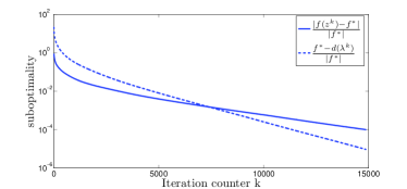
(a) Primal and dual suboptimality along iterations.

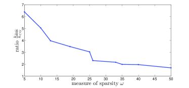
(b) Ratio $k_{DG}/k_{CG}$ w.r.t. sparsity measure $\omega$.

Figure 1: Behavior of Algorithm (DG).

In this section we consider problems of the form (1), where the objective functions are given by:

$$f_{i}(z_{i})=0.5\|z_{i}\|_{Q_{i}}^{2}+q_{i}^{T}z_{i}+\gamma_{i}\log\left(1+e^{\langle a_{i},z_{i}\rangle}\right).$$

Note that this type of function satisfies Assumption 2.1 (a), provided that $Q_{i}$ are positive definite matrices, and are intensively used in (DMPC) applications for $\gamma_{i}=0$ or (NUM) applications for $\gamma_{i}>0$. We first generate a sparse communication graph $\mathcal{G}=\left(V,E\right)$ characterized by an incidence matrix $E\in\mathbb{R}^{M\times M}$ generated randomly with different degrees of sparsity given by $\bar{\mathcal{N}}_{i}$ and $\mathcal{N}_{j}$. Recall that we have defined the measure of sparsity of the incidence matrix $E$ as: $\omega=\max_{i,j\in V}\left\{|\bar{\mathcal{N}}_{i}|,|\mathcal{N}_{j}|\right\}$. We take $n_{i}=n_{j}$ for all $i,j$. Matrices $Q_{i}\in\mathbb{R}^{n_{i}\times n_{i}}$, $A_{ji}\in\mathbb{R}^{\lceil\frac{3n_{i}}{4}\rceil\times n_{i}}$ and $C_{ji}\in\mathbb{R}^{\lceil\frac{3n_{i}}{2}\rceil\times n_{i}}$ are taken from a normal distribution with zero mean and unit variance. Matrix $Q_{i}$ is then made positive definite by transformations $Q_{i}\leftarrow Q_{i}^{T}Q_{i}+\sigma_{i}I_{n_{i}}$, where $\sigma_{i}$ are randomly generated from the interval $[1,10]$. Further, vectors $b$, $c$ are chosen such that the problem is feasible, and $q_{i}$ and $a_{i}$ are taken from an uniform distribution and $\gamma_{i}=1$ for all $i$.

In order to analyze the behavior of Algorithm (DG) we first consider a problem with the number of subsystems $M=100$, the dimension of local variables $n_{i}=10$ for all $i\in\left\{1,\dots,100\right\}$ and $\omega=15$. We are interested in analyzing the evolution of both, primal and dual suboptimality, w.r.t. the number of iterations. We consider an accuracy $\epsilon=10^{-4}$ and impose a stopping criterion of the form:

$$\frac{|f(z^{k})-f^{*}|}{|f^{*}|}\leq\epsilon,$$ (42)

where $f^{*}$ is computed using CVX. We plot the results in logarithmic scale in Figure 1a. We can observe that both dual and primal suboptimality converge linearly, which confirms the theoretical results derived in Section 4. Moreover, in one of our recent papers [17] we have proved that dual gradient algorithm in the last primal iterate is converging sublinearly (order $\mathcal{O}(1/\sqrt{k})$) in terms of primal suboptimality and infeasibility, provided that the primal objective function $f$ is only strongly convex (i.e. $f$ has not Lipschitz gradient and thus no error bound property holds for the dual problem). In particular, we have proved that primal suboptimality is of order $\mathcal{O}(\frac{\mathcal{R}^{2}(\lambda^{0})}{\sqrt{k}})$ and primal infeasibility is of order $\mathcal{O}(\frac{\mathcal{R}(\lambda^{0})}{\sqrt{k}})$. From Figure 2 we again observe linear convergence. In the same figure we also plot the theoretical sublinear estimates for the convergence rate of order $\mathcal{O}(1/\sqrt{k})$ for Algorithm (DG) in the last iterate as described above (see [17] for more details). The plot clearly confirms our theoretical findings, i.e. linear convergence of Algorithm (DG) in the last iterate.

We are also interested in comparing the performances of Algorithm (DG) with the ones of the centralized dual gradient method, called Algorithm (CG), where for updating the dual variable $\lambda$ we use the centralized step size $L_{\text{d}}^{-1}I_{p+q}$ (see also [15]):

$$(\textbf{CG}):\quad{\lambda}^{k+1}=\left[\lambda^{k}+L_{\text{d}}^{-1}\nabla d(\lambda^{k})\right]_{\mathbb{D}}.$$

For this purpose, we consider a set of 10 problems with fixed dimension, $M=100$ and $n=10$, accuracy $\epsilon=10^{-2}$ and the measure of sparsity $\omega$ ranging from $5$ to $50$. We plot in Figure 1b the ratio between the number of iterations performed by Algorithm (DG) ($k_{DG}$) and by Algorithm (CG) ($k_{CG}$), respectively. On the one hand, we observe that for small values of the sparsity measure $\omega$, Algorithm (DG) clearly outperforms Algorithm (CG). On the other hand, by increasing the sparsity measure $\omega$ we observe a reduction in the ratio between the number of iterations performed by the two algorithms.

Further, we consider problems of different dimensions, having the measure of sparsity $\omega=0.15M$, and compare the Algorithms (DG) and (CG) in terms of number of iterations performed for obtaining a suboptimal solution with accuracy $\epsilon=10^{-2}$. In Table 1 we present the average results obtained for 10 randomly generated problems for each dimension. We use the notation $\overline{w}=\lambda_{\text{max}}(W)$ and we recall that $\underline{w}=\lambda_{\text{min}}(W)$. We can observe that for all dimensions, Algorithm (DG) outperforms Algorithm (CG) due to the reduced level of sparsity $\omega$ and smaller values of the entries of weighted step size $W$ compared to the centralized one $L_{\text{d}}$.

	$(200,10)$	$(100,20)$	(50,40)
$k_{DG}$	3861	4117	4936
$k_{CG}$	16121	19541	27973
$L_{\text{d}}$	691	802	1346
$\overline{w}$	653	854	1433
$\underline{w}$	21	49	79

Table 1: Average number of iterations for finding an $\epsilon$-solution.

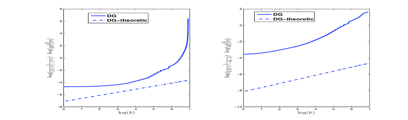
(a) Linear convergence of Algorithm (DG) in the last iterate: logarithmic scale of primal suboptimality and infeasibility. We also compare with the theoretical sublinear estimates (dot lines) for the convergence rate of order ${\mathcal{O}}(1/\sqrt{k})$. The plot clearly shows our theoretical findings, i.e. linear convergence.

Figure 2: Algorithm (DG): theoretical vs. practical behavior.

7 Conclusions

In this paper we have proposed and analyzed a fully distributed dual gradient method for solving the Lagrangian dual of a primal separable convex optimization problem with linear constraints. Under the strong convexity and Lipschitz continuous gradient property assumptions of the primal objective function we have provided a global error bound for the dual problem. Using this property, we have proved global linear convergence rate for both primal and dual suboptimality and for primal feasibility violation for our distributed dual gradient algorithm. We have also discussed distributed implementation aspects for our method and provided several numerical simulations which confirm the theoretical results and the efficiency of our approach.

Appendix

In order to prove Theorem 3.2 we first need some technical results. First we recall from Lemma 3.1 that there exists a unique $y^{*}\in\mathbb{R}^{n}$ such that:

$$G^{T}\lambda^{*}=y^{*}\quad\forall\lambda^{*}\in\Lambda^{*}.$$

Moreover, $\nabla d(\lambda)=G\nabla\tilde{f}(-y^{*})-g$ is constant for all $\lambda\in\Lambda$, where we have defined the set:

$$\Lambda=\left\{\lambda\in\mathbb{D}:G^{T}\lambda=y^{*}\right\}.$$

We introduce further the following notations:

$$r=\left[\lambda\right]_{\Lambda}^{W}~{}\text{and}~{}\bar{r}=\left[r\right]_{\Lambda^{*}}^{W}\qquad\forall\lambda\in\mathbb{D}.$$ (43)

Using now the notations (43) and $\bar{\lambda}=\left[\lambda\right]_{\Lambda^{*}}^{W}$ we can write:

$$\|\lambda-\bar{\lambda}\|^{2}_{W} \!\leq\left\|\lambda-\bar{r}\right\|^{2}_{W}\leq\left(\|\lambda-r\|_{W}+\|r-\bar{r}\|_{W}\right)^{2}$$

$$\!\leq 2\|\lambda-r\|_{W}^{2}\!+2\|r-\bar{r}\|^{2}_{W}\quad\forall\lambda\in\mathbb{D}.$$ (44)

In what follows we show how we can find upper bounds on $\|\lambda-r\|_{W}$ and $\|r-\bar{r}\|_{W}$ such that we will be able to establish the error bound property on the dual problem (2) given in Theorem 3.2.

Lemma 7.1.

Let Assumption 2.1 hold and $\nabla^{+}d$ given in (16). Then, the following inequality holds for all $\lambda,\omega\in\mathbb{D}$:

$$\langle\nabla d(\omega)-\nabla d(\lambda),\!\lambda-\omega\rangle\!\!\leq\!2\|\nabla^{+}\!d(\lambda)-\nabla^{+}\!d(\omega)\|_{W}\;\|\lambda-\omega\|_{W}.$$

First, let us recall that $\left[\lambda+W^{-1}\nabla d(\lambda)\right]^{W}_{\mathbb{D}}$ is the unique solution of the optimization problem:

$$\min_{\xi\in\mathbb{D}}\|\xi-\lambda-W^{-1}\nabla d(\lambda)\|_{W}^{2},$$ (45)

for which the optimality conditions reads:

$$\!\!\!\!\!\!\!\left\langle W\!\left(\!\left[\lambda\!+\!W^{-1}\nabla d(\lambda)\right]^{W}_{\mathbb{D}}\!\!-\!\left(\!\lambda\!+\!W^{-1}\nabla d(\lambda)\right)\!\!\right),\right.$$

$$\qquad\qquad\left.\xi-\left[\lambda\!+\!W^{-1}\nabla d(\lambda)\right]^{W}_{\mathbb{D}}\right\rangle\geq 0\quad\forall\xi\in\mathbb{D}.$$

Taking now $\xi=\left[\omega+W^{-1}\nabla d(\omega)\right]^{W}_{\mathbb{D}}$ in the previous inequality, adding and subtracting both, $\lambda$ and $\omega$, in the right term of the scalar product and using the definition of $\nabla^{+}d$ we obtain:

$$\langle W\!\left(\nabla^{+}\!d(\lambda)\!-\!W^{-1}\nabla d(\lambda)\right)\!,\!\nabla^{+}\!d(\lambda)+\lambda-\omega-\nabla^{+}\!d(\omega)\rangle\!\!\leq\!0,$$

and the symmetry of matrix $W$ leads to:

$$\langle\nabla^{+}d(\lambda)-W^{-1}\nabla d(\lambda),$$

$$\qquad\qquad~{}~{}W\left(\lambda-\omega\right)+W\left(\nabla^{+}d(\lambda)-\nabla^{+}d(\omega)\right)\rangle\leq 0.$$

Rearranging the terms in the previous inequality we get:

$$- \langle\nabla d(\lambda),\lambda-\omega\rangle$$

$$\leq\!\!-\langle\nabla^{+}d(\lambda),W\!(\lambda\!-\!\omega)\rangle\!+\!\langle\nabla d(\lambda),\nabla^{+}d(\lambda)\!-\!\nabla^{+}d(\omega)\rangle$$

$$\qquad\qquad-\langle\nabla^{+}d(\lambda),W\left(\nabla^{+}d(\lambda)-\nabla^{+}d(\omega)\right)\rangle.$$

Writing now the previous inequality with $\lambda$ and $\xi$ interchanged and summing them up we can write:

$$\langle\nabla d(\xi)\!-\!\nabla d(\lambda),\lambda\!-\!\xi\rangle$$

$$\leq\!\langle\nabla^{+}\!d(\xi)\!-\!\nabla^{+}\!d(\lambda),W(\lambda\!-\!\xi)\rangle\!$$

$$\qquad+\langle\nabla d(\lambda)\!-\!\nabla d(\xi),\nabla^{+}\!d(\lambda)\!-\!\nabla^{+}\!d(\xi)\rangle\!$$

$$\qquad-\!\|\nabla^{+}d(\lambda)\!-\!\nabla^{+}d(\xi)\|_{W}^{2}$$

$$\leq\langle\nabla^{+}\!d(\xi)\!-\!\nabla^{+}\!d(\lambda),W(\lambda\!-\!\xi)\rangle\!$$

$$\qquad+\langle\nabla d(\lambda)\!-\!\nabla d(\xi),\nabla^{+}\!d(\lambda)-\nabla^{+}d(\xi)\rangle$$

$$\leq\|\nabla^{+}d(\lambda)-\nabla^{+}d(\xi)\|_{W}\|W(\lambda-\xi)\|_{W^{-1}}$$

$$\qquad+\|\nabla^{+}d(\lambda)-\nabla^{+}d(\xi)\|_{W}\|\nabla d(\lambda)-\nabla d(\xi)\|_{W^{-1}}$$

$$\leq 2\|\nabla^{+}d(\lambda)-\nabla^{+}d(\xi)\|_{W}\|\lambda-\xi\|_{W},$$

which concludes the statement. ∎

The next lemma gives un upper bound on $\|\lambda-r\|_{W}$:

Lemma 7.2.

Under Assumption 2.1 there exists a constant $\kappa_{1}$ such that the following inequality holds:

$$\|\lambda-r\|^{2}_{W}\leq\kappa_{1}\;\|\nabla^{+}d(\lambda)\|_{W}\;\|\lambda-\bar{\lambda}\|_{W}\quad\forall\lambda\in\mathbb{D},$$ (46)

where $\kappa_{1}=\frac{2}{\sigma_{\tilde{\mathrm{f}}}}\theta_{1}^{2}$ and $\theta_{1}$ depends on the matrix $G$.

First, let us notice that we can write the set $\Lambda$ explicitly as:

$$\Lambda =\left\{\omega\in\mathbb{R}^{p+q}:~{}F\omega\leq 0,~{}~{}G^{T}\omega=y^{*}\right\},$$ (47)

where $F=\left[0_{q,p}~{}-I_{q}\right]$. Since $\lambda\in\mathbb{D}$, it implies $F\lambda\leq 0$ and therefore, according to Theorem 2 in [25], we can bound the distance between a vector $\lambda$ and the polyhedron $\Lambda$ as follows:

$$\|\lambda-r\|_{W}\leq\theta_{1}\|G^{T}\lambda-y^{*}\|_{\infty}\leq\theta_{1}\|G^{T}\lambda-y^{*}\|,$$ (48)

where $\theta_{1}$ is the Hoffman’s bound depending on the matrix $G$ and on the norms $\|\cdot\|_{W}$ and $\|\cdot\|_{\infty}$ (see eq. (6) in [25] for a formula to compute Hoffman’s bound). From the strong convexity property of $\tilde{f}$ combined with the fact that $G^{T}\bar{\lambda}=y^{*}$ we have:

$$\sigma_{\tilde{\mathrm{f}}}\|G^{T}\lambda-y^{*}\|^{2}$$ (49)

$$\leq\langle\nabla\tilde{f}(-G^{T}\lambda)-\nabla\tilde{f}(-G^{T}\bar{\lambda}),-G^{T}\lambda+G^{T}\bar{\lambda}\rangle$$

$$=\langle-G\nabla\tilde{f}(-G^{T}\lambda)+g+G\nabla\tilde{f}(-G^{T}\bar{\lambda})-g,\lambda-\bar{\lambda}\rangle$$

$$=\langle\nabla d(\bar{\lambda})-\nabla d(\lambda),\lambda-\bar{\lambda}\rangle$$

$$\leq 2\|\nabla^{+}d(\lambda)-\nabla^{+}d(\bar{\lambda})\|_{W}\|\lambda-\bar{\lambda}\|_{W}$$

$$=2\|\nabla^{+}d(\lambda)\|_{W}\|\lambda-\bar{\lambda}\|_{W},$$

where the last inequality follows from Lemma 7.1 and the last equality follows from the fact that $\nabla^{+}d(\bar{\lambda})=0$ for $\bar{\lambda}\in\Lambda^{*}$. Combining now (48) with (49) we obtain the result. ∎

The next result establishes an upper bound on $\|r-\bar{r}\|_{W}$:

Lemma 7.3.

Let Assumption 2.1 be satisfied. Then, the following inequality is valid:

$$\|r-\bar{r}\|_{W}^{2}\!\leq\!\kappa_{2}(\mathcal{T}(\lambda))\|\nabla^{+}\!d(\lambda)\|_{W}\|\lambda-\bar{\lambda}\|_{W}\!\!\!\quad\forall\lambda\!\in\!\mathbb{D},$$ (50)

where $r,\bar{r}$ are given in (43), $\bar{\lambda}=\left[\lambda\right]_{\Lambda^{*}}^{W}$ and

$$\kappa_{2}(\mathcal{T}(\lambda))\!=6\theta_{2}^{2}\left(2\mathcal{T}^{2}(\lambda)+2\|\nabla d(\bar{\lambda})\|_{W^{-1}}^{2}\right)\!\left(1\!+\!3\theta_{1}^{2}\frac{2}{\sigma_{\tilde{\mathrm{f}}}}\right),$$

with $\mathcal{T}(\lambda)=\max\limits_{\lambda^{*}\in\Lambda^{*}}\|\lambda-\lambda^{*}\|_{W}$ and $\theta_{2}$ being a constant depending on $C$, $\nabla d(\bar{\lambda})$ and $y^{*}$.

Since $\Lambda^{*}\subseteq\Lambda\subseteq\mathbb{D}$ and $G^{T}\xi=y^{*}$ for all $\xi\in\Lambda$, the dual problem (2) has the same optimal solutions as the following linear program:

$$\arg\max_{\lambda\in\mathbb{D}}d(\lambda) \!=\!\arg\max_{\xi\in\Lambda}d(\xi)\!=\!\arg\max_{\xi\in\Lambda}-\tilde{f}(-y^{*})-\langle g,\xi\rangle$$

$$\!=\!\arg\max_{\xi\in\Lambda}-\langle g,\xi\rangle.$$ (51)

Further, let us recall that $\nabla d(\zeta)=G\nabla\tilde{f}(-y^{*})-g$ for any $\zeta\in\Lambda$ and thus we have that $\langle\nabla d(\zeta),\xi\rangle=\langle\nabla\tilde{f}(-y^{*}),y^{*}\rangle-\langle g,\xi\rangle$ for all $\zeta,\xi\in\Lambda$. Therefore, we can write further for any $\zeta\in\Lambda$:

$$\arg\max_{\xi\in\Lambda}\langle\nabla d(\zeta),\xi\rangle =\arg\max_{\xi\in\Lambda}\langle\nabla\tilde{f}(-y^{*}),y^{*}\rangle-\langle g,\xi\rangle$$

$$=\arg\max_{\xi\in\Lambda}-\langle g,\xi\rangle.$$ (52)

Combining now (Appendix) with (Appendix), we can conclude that any solution of the dual problem (2) $\bar{\xi}=[\xi]_{\Lambda^{*}}^{W}$, with $\xi\in\Lambda$, is also a solution of linear program (Appendix). Since $\Lambda^{*}\subseteq\Lambda$, then for any $\left[\lambda\right]_{\Lambda^{*}}^{W}=\bar{\lambda}\in\Lambda^{*}$ we have that $\nabla_{\nu}d(\bar{\lambda})=Az^{*}-b=0$ and $\nabla_{\mu}d(\bar{\lambda})=Cz^{*}-c\leq 0$, and thus we also have that the maximum in (Appendix) is finite for any $\zeta=\bar{\lambda}=\left[\lambda\right]_{\Lambda^{*}}^{W}\in\Lambda^{*}$. Thus problem (Appendix) is solvable for any $\zeta=\bar{\lambda}=\left[\lambda\right]_{\Lambda^{*}}^{W}\in\Lambda^{*}$. Applying now Theorem 2 in [25] to the optimality conditions of problem (Appendix) and its dual we obtain:

$$\|\xi-\bar{\xi}\|_{W}\leq\theta_{2}|\langle\nabla d(\bar{\lambda}),\xi\rangle-\langle\nabla d(\bar{\lambda}),\bar{\xi}\rangle|\quad\forall\xi\in\Lambda,$$ (53)

where $\theta_{2}$ is Hoffman’s bound depending only on the matrix $C$ and vectors $\nabla d(\bar{\lambda})$ and $y^{*}$ (see eq. (6) in [25] for details). Using the previous relation we have:

$$\|\xi-\bar{\xi}\|_{W} \leq\theta_{2}|\langle\nabla d(\bar{\lambda}),\xi\rangle-\langle\nabla d(\bar{\lambda}),\bar{\xi}\rangle|$$

$$=\theta_{2}\langle\nabla d(\bar{\lambda}),\bar{\xi}-\xi\rangle.$$ (54)

For any $\xi\in\Lambda$ the optimality conditions of the following projection problem $\min\limits_{\omega\in\Lambda}\|\omega-\xi-W^{-1}\nabla d(\bar{\lambda})\|_{W}^{2}$ become:

$$\!\!\!\!\!\!\!\!\!\left\langle W\left(\left[\xi+W^{-1}\nabla d(\bar{\lambda})\right]_{\Lambda}^{W}-\xi-W^{-1}\nabla d(\bar{\lambda})\right),\right.$$

$$\qquad\qquad\left.\left[\xi+W^{-1}\nabla d(\bar{\lambda})\right]_{\Lambda}^{W}-\omega\right\rangle\leq 0,~{}~{}\forall\omega\in\Lambda.$$

Taking now $\omega=\bar{\xi}=[\xi]^{W}_{\Lambda^{*}}$ and since $W$ is a symmetric matrix we obtain:

$$\langle\nabla d(\bar{\lambda}),\bar{\xi}\!-\!\xi\rangle$$

$$\leq\left\langle\left[\xi\!+\!W^{-1}\nabla d(\bar{\lambda})\right]_{\Lambda}^{W}\!\!\!-\!\xi,\right.$$

$$\quad\qquad\qquad\qquad\left.W\!\left(\bar{\xi}\!-\!\left[\xi\!+\!W^{-1}\nabla d(\bar{\lambda})\right]_{\Lambda}^{W}\right)\!+\!\nabla d(\bar{\lambda})\right\rangle$$

$$=\!\left\langle\left[\xi\!+\!W^{-1}\nabla d(\bar{\lambda})\right]_{\Lambda}^{W}\!\!-\xi,\right.$$

$$~{}\quad\quad\left.W\!\left(\xi\!-\!\left[\xi\!+\!W^{-1}\nabla d(\bar{\lambda})\right]_{\Lambda}^{W}\right)+W(\bar{\xi}\!-\!\xi)\!+\!\nabla d(\bar{\lambda})\right\rangle$$

$$\leq\langle\left[\xi+W^{-1}\nabla d(\bar{\lambda})\right]_{\Lambda}^{W}-\xi,W(\bar{\xi}-\xi)+\nabla d(\bar{\lambda})\rangle$$

$$\leq\left\|\left[\xi+W^{-1}\nabla d(\bar{\lambda})\right]_{\Lambda}^{W}-\xi\right\|_{W}\|W(\bar{\xi}-\xi)\|_{W^{-1}}$$

$$\qquad+\left\|\left[\xi+W^{-1}\nabla d(\bar{\lambda})\right]_{\Lambda}^{W}-\xi\right\|_{W}\|\nabla d(\bar{\lambda})\|_{W^{-1}}$$

$$=\|\nabla^{+}d(\xi)\|_{W}\left(\|\xi-\bar{\xi}\|_{W}+\|\nabla d(\bar{\lambda})\|_{W^{-1}}\right),$$

where in the last equality we used the definition of $\nabla^{+}d$ and the fact that $\nabla d(\bar{\lambda})=\nabla d(\xi)$ for all $\xi\in\Lambda$ (see Lemma 3.1). Combining now the previous inequality with (Appendix) and taking $\xi=r\in\Lambda$ we obtain:

$$\|r\!-\!\bar{r}\|_{W}^{2}\!\!\leq\!\!\theta_{2}^{2}\!\!\left(\|r\!-\!\bar{r}\|_{W}\!\!+\!\!\|\nabla d(\bar{\lambda})\|_{W^{-1}}\!\right)^{2}\!\|\nabla^{+}\!d(r)\|_{W}^{2}.$$ (55)

Since $\bar{r}=\left[r\right]_{\Lambda^{*}}^{W}$ and $\Lambda^{*}\subseteq\Lambda$ we also have $\bar{r}=\left[\bar{r}\right]_{\Lambda}^{W}$. Thus, using the nonexpansive property of the projection we can bound the term $\|r-\bar{r}\|_{W}$ from above with a finite positive constant $\mathcal{T}(\lambda)=\max\limits_{\lambda^{*}\in\Lambda^{*}}\|\lambda-\lambda^{*}\|_{W}$:

$$\|r-\bar{r}\|_{W}\leq\|\lambda-\bar{r}\|_{W}\leq\max\limits_{\lambda^{*}\in\Lambda^{*}}\|\lambda-\lambda^{*}\|_{W}=\mathcal{T}(\lambda).$$ (56)

Note that $\mathcal{T}(\lambda)$ is finite for any $\lambda\in\mathbb{D}$, provided that $\Lambda^{*}$ is a bounded set. Further, our goal is to find an upper bound for $\|\nabla^{+}d(r)\|_{W}$ in terms of $\|\lambda-\bar{\lambda}\|_{W}$ and $\|\nabla^{+}d(\lambda)\|_{W}$. To this purpose, let us first prove that $\nabla^{+}d$ is Lipschitz continuous with constant $3$ w.r.t. the norm $\|\cdot\|_{W}$. For any $\lambda,\tilde{\lambda}\in\mathbb{D}$ we can write:

$$\|\nabla^{+}d(\lambda)\!-\!\nabla^{+}d(\tilde{\lambda})\|_{W}\leq\|\lambda\!-\!\tilde{\lambda}\|_{W}$$ (57)

$$\qquad\qquad+\left\|\left[\lambda\!+\!W^{-1}\nabla d(\lambda)\right]_{\mathbb{D}}^{W}-\left[\tilde{\lambda}\!+\!W^{-1}\nabla d(\tilde{\lambda})\right]_{\mathbb{D}}^{W}\right\|$$

$$\leq\|\lambda\!-\!\tilde{\lambda}\|_{W}\!+\!\|\lambda+W^{-1}\nabla d(\lambda)\!-\!\tilde{\lambda}\!-\!W^{-1}\nabla d(\tilde{\lambda})\|_{W}$$

$$\leq 2\|\lambda-\tilde{\lambda}\|_{W}+\|\nabla d(\lambda)-\nabla d(\tilde{\lambda})\|_{W^{-1}}\leq 3\|\lambda-\tilde{\lambda}\|_{W}.$$

Using now (57) with $\tilde{\lambda}=\bar{\lambda}$ and taking into account that $\nabla^{+}d(\bar{\lambda})=0$, we have:

$$\|\nabla^{+}\!d(\lambda)\|_{W}\!=\!\|\nabla^{+}d(\lambda)\!-\!\nabla^{+}d(\bar{\lambda})\|_{W}\!\leq\!3\|\lambda\!-\!\bar{\lambda}\|_{W}.$$

Using now again (57) and the previous inequality we get:

$$\|\nabla^{+}\!d(r)\|_{W}^{2} \!\leq\left(\|\nabla^{+}d(\lambda)\|_{W}\!+\!\|\nabla^{+}d(r)\!-\!\nabla^{+}d(\lambda)\|_{W}\right)^{2}$$

$$\!\leq 2\|\nabla^{+}d(\lambda)\|_{W}^{2}+2\|\nabla^{+}d(r)-\nabla^{+}d(\lambda)\|_{W}^{2}$$

$$\!\leq 6\|\nabla^{+}d(\lambda)\|_{W}\|\lambda-\bar{\lambda}\|_{W}+18\|\lambda-r\|_{W}^{2}$$

$$\!\leq 6\!\left[1\!+\!3\theta_{1}^{2}\frac{2}{\sigma_{\tilde{\mathrm{f}}}}\right]\!\|\nabla^{+}\!d(\lambda)\|_{W}\|\lambda\!-\!\bar{\lambda}\|_{W},$$ (58)

where in the last inequality we used (46). Introducing now (56) and (Appendix) in (55) and using the inequality $(\alpha+\beta)^{2}\leq 2\alpha^{2}+2\beta^{2}$ we obtain the result. ∎

(Proof of Theorem 3.2) The result given in Theorem 3.2 follows immediately by using (46) from Lemma 7.2 and (50) from Lemma 7.3 in (Appendix) and dividing both sides by $\|\lambda-\bar{\lambda}\|_{W}$. ∎

References

• [1] A.G. Bakirtzis and P.N. Biskas. A decentralized solution to the dc-opf of interconnected power systems. IEEE Transactions on Power Systems, 18(3):1007–1013, 2003.
• [2] A. Beck, A. Nedic, A. Ozdaglar, and M. Teboulle. Optimal distributed gradient methods for network resource allocation problems. IEEE Transactions on Control of Network Systems, to appear, 2014.
• [3] M.D. Doan, T. Keviczky, and B. De Schutter. A distributed optimization-based approach for hierarchical mpc of large-scale systems with coupled dynamics and constraints. In Proceedings of 50th Conference on Decision and Control, pages 5236–5241, 2011.
• [4] F. Facchinei and J-S. Pang. Finite–dimensional variational inequalities and complementarity problems, volume Springer Series in Operations Research. Springer–Verlag, NY, 2003.
• [5] M. Farina and R. Scattolini. Distributed predictive control: a non-cooperative algorithm with neighbor-to-neighbor communication for linear systems. Automatica, 48(6):1088–1096, 2012.
• [6] P. Giselsson, M. D. Doan, T. Keviczky, B. De Schutter, and A. Rantzer. Accelerated gradient methods and dual decomposition in distributed model predictive control. Automatica, 49:829–833, 2013.
• [7] J.B. Hiriart-Urruty and C. Lemarechal. Convex analysis and minimization algorithms: vol. I. Springer-Verlag, 1996.
• [8] M. Hong and Z.Q. Luo. On the linear convergence of the alternating direction method of multipliers. Technical Report arxiv preprint: 1208.3922, 2013.
• [9] M. Kogel and R. Findeisen. Fast predictive control of linear systems combining nesterov’s gradient method and the method of multipliers. In Proceedings of 50th Conference on Decision and Control, pages 501–506, 2011.
• [10] Z.Q. Luo and P. Tseng. Error bounds and convergence analysis of feasible descent methods: A general approach. Annals of Operations Research, 46–47(1):157–178, 1993.
• [11] Z.Q. Luo and P. Tseng. On the convergence rate of dual ascent methods for linearly constrained convex minimization. Mathematics of Operations Research, 18(4):846–867, 1993.
• [12] D.Q. Mayne, J.B. Rawlings, C.V. Rao, and P.O.M. Scokaert. Constrained model predictive control: Stability and optimality. Automatica, 36(6):789–814, 2000.
• [13] M.C. Meinel, M. Ulbrich, and S. Albrecht. A class of distributed optimization methods with event-triggered communication. Computational Optimization and Applications, 57:517–553, 2014.
• [14] I. Necoara and D. Clipici. Efficient distributed coordinate descent methods on smooth and error bound convex minimization. SIAM J. Optimization, submitted, 2013.
• [15] I. Necoara and V. Nedelcu. Rate analysis of inexact dual first order methods: application to dual decomposition. IEEE Transactions on Automatic Control, 59(5):1232–1243, 2014.
• [16] I. Necoara, V. Nedelcu, and I. Dumitrache. Parallel and distributed optimization methods for estimation and control in networks. Journal of Process Control, 21(5):756–766, 2011.
• [17] I. Necoara and A. Patrascu. Iteration complexity analysis of dual first order methods for convex programming. Technical report, University Politehnica Bucharest, June 2014.
• [18] I. Necoara and J.A.K. Suykens. Application of a smoothing technique to decomposition in convex optimization. IEEE Transactions on Automatic Control, 53(11):2674–2679, 2008.
• [19] I. Necoara and J.A.K. Suykens. An interior-point lagrangian decomposition method for separable convex optimization. Journal of Optimization Theory and Applications, 143(3):567–588, 2009.
• [20] V. Nedelcu, I. Necoara, and D. Q. Quoc. Computational complexity of inexact gradient augmented lagrangian methods: application to constrained mpc. SIAM Journal on Control and Optimization, to appear:1–26, 2014.
• [21] A. Nedic and A. Ozdaglar. Approximate primal solutions and rate analysis for dual subgradient methods. SIAM Journal on Optimization, 19(4):1757–1780, 2009.
• [22] Y. Nesterov. Introductory Lectures on Convex Optimization: A Basic Course. Kluwer, Boston, USA, 2004.
• [23] J.-S. Pang. A posteriori error bounds for the linearly constrained variational inequality problem. Mathematics Of Operations Research, 12(3):474–484, 1987.
• [24] P. Patrinos and A. Bemporad. An accelerated dual gradient-projection algorithm for embedded linear MPC. IEEE Transactions on Automatic Control, 59(1):18–33, 2014.
• [25] S. M. Robinson. Bounds for error in the solution set of a perturbed linear program. Linear Algebra and its Applications, 6:69–81, 1973.
• [26] R.T. Rockafellar and R.J. Wets. Variational Analysis. Springer-Verlag, New York, 1998.
• [27] S. Sen and H.D. Sherali. A class of convergent primal-dual subgradient algorithms for decomposable convex programs. Mathematical Programming, 35(3):279–297, 1986.
• [28] P.W. Wang and C.J. Lin. Iteration complexity of feasible descent methods for convex optimization. Technical report, National Taiwan University, 2013.
• [29] E. Wei and A. Ozdaglar. On the o(1/k) convergence of asynchronous distributed alternating direction method of multipliers. Technical report, MIT, 2013.
• [30] E. Wei, A. Ozdaglar, and A. Jadbabaie. A distributed newton method for network utility maximization – part I and II. IEEE Transactions on Automatic Control, 58(9), 2013.