Linear programming analysis of the -parity violation within EDM-constraints
Abstract
The constraint on the -parity violating supersymmetric interactions is discussed in the light of current experimental data of the electric dipole moment of neutron, 129Xe , 205Tl, and 199Hg atoms, and YbF and ThO molecules. To investigate the constraints without relying upon the assumption of the dominance of a particular combination of couplings over all the rest, an extensive use is made of the linear programming method in the scan of the parameter space. We give maximally possible values for the EDMs of the proton, deuteron, 3He nucleus, 211Rn, 225Ra, 210Fr, and the -correlation of the neutron beta decay within the constraints from the current experimental data of the EDMs of neutron, 129Xe, 205Tl, and 199Hg atoms, and YbF and ThO molecules using the linear programming method. It is found that the -correlation of the neutron beta decay and hadronic EDMs are very useful observables to constrain definite regions of the parameter space of the -parity violating supersymmetry.
pacs:
12.60.Jv, 11.30.Er, 13.40.Em, 14.80.LyI Introduction
The supersymmetric (SUSY) extension of the Standard Model (SM) has widely been discussed as a good candidate of the new physics mssm . One of the important aspects of the supersymmetric SM is that it allows room for baryon and lepton number violation. The conservation of -parity is often introduced to forbid such violation. We must say, however, that this conservation has never been put on a strong convincing basis, and many phenomenological analyses of the -parity violation were done so far rpvphenomenology .
In spite of dedicated efforts in LHC experiment, an evidence of suparparticles is yet to come. The LHC data have so far placed only tight constraints on the SUSY parameter space. It is to be noted, however, that most of the SUSY analyses of LHC results have been performed, assuming the -parity conservation. If this assumption is relaxed, decay modes of superparticles become different and the constrained parameter space could be significantly altered. The principal reason for our renewed interest in RPV SUSY models is to extend the scope of looking at LHC data and of groping our way towards new physics.
One of the promising experimental approach to search for new physics beyond the SM is the electric dipole moment (EDM) edmreview ; khriplovichbook ; ginges ; pospelovreview ; yamanakabook . The advantages of the EDM are almost obvious and far-reaching. Namely, the EDM can be measured with high accuracy in a variety of systems. The representative experimental data are the EDMs of 129Xe atom () rosenberry , 205Tl atom () regan , neutron () baker , 199Hg atom () griffith , muon () muong2 , YbF molecule () hudson , ThO molecule () acme . There are also many future experimental prospects such as the measurement of the EDMs of proton storage ; bnl , deuteron storage ; bnl , muon storage ; bnl , 225Ra atom mueller , neutron ucn , 129Xe atom xeasahi , 210Fr atom sakemi , etc. All these EDMs are expected to receive very small contributions from SM smedm , which makes them to be an excellent probe of the new physics. The EDM is so sensitive to the new physics that the supersymmetric models with susyedm1-loop ; susyedm2-loop ; susyedmgeneral ; falk ; hisano ; degrassi ; susyedmflavorchange ; yamanakarainbow1 ; pospelovreview ; ellisgeometricapproach ; dekens and without -parity barbieri ; godbole ; chang ; herczege-n ; choi ; cch ; faessler ; yamanaka1 ; rpvedmsfermion have been analyzed to a considerable extent, and many supersymmetric CP phases were constrained so far.
The parameter space of the -parity violation is quite large, and the analysis of the whole parameter space including the usual -parity conserving parameters is discouragingly difficult. In such situations, we often restrict the parameter space only to few parameters to allow for feasible phenomenological analyses, as done in many previous works (under the assumptions of a single coupling dominance), and many tight constraints on the RPV couplings have been derived so far. This approach assuming a single coupling dominance, however, cannot exhaust all corners of the RPV parameter space in which interferences could occur, and thereby some couplings may be sufficiently larger than upper limits derived with this assumption. In the -parity conserving sector, a systematic analysis of the SUSY CP phases was done by Ellis et al. (for the minimally flavor violating maximally CP violating model), and they obtained a possible large prediction for many prepared experiments such as the EDMs of the deuteron or 225Ra atom ellisgeometricapproach . If the supersymmetric theory is extended with RPV, an equally full analysis for RPV interactions seems to be needed. Our aim is then to do a systematic analysis of the full space of the CP violating RPV interactions on the basis of the linear programming method by using the constraints due to the existing experimental data (neutron, 129Xe, 205Tl, 199Hg, YbF and ThO EDMs plus other CP conserving experimental data of fundamental precision tests rpvphenomenology ), and to present the maximal expectations for P, CP-odd observables in preparation. In the present analysis, we will predict the EDMs of the proton, deuteron, 3He nucleus, 210Fr, 211Rn, 225Ra atoms, muon, and the -correlation of the neutron beta decay with the linear programming method.
This paper is organized as follows. We first present in Section II the RPV interactions and their contribution to the EDM observables. The elementary level RPV processes as well as the hadronic and many-body physics needed in the computation are explained in detail. We then give a brief review of the linear programming algorithm in Section III. In Section IV, we provide the whole setup of the input parameters. There the complete formulae of the EDMs used in this analysis are shown. We then analyze the constraints to RPV couplings in Section V, and also the prospective values of the future EDM experiments. The last part is devoted to the summary.
II RPV contributions to the EDMs
II.1 Elementary level contribution
We first review the RPV contribution at the elementary level. The derivation of the RPV contribution to the EDM observables is based on our previous papers yamanaka1 ; rpvedmsfermion .
The RPV superpotential relevant in our discussion is the following:
| (1) |
with indicating the generation, the indices. and denote the lepton doublet and singlet left-chiral superfields, respectively. and denote respectively the quark doublet and down quark singlet left-chiral superfields.
In the presence of the bilinear RPV interactions, the authors of choi made a suitable use of the flavor basis in which only one of the four doublet fields bears vacuum expectation value SVP . In this work, however, we assume that the bilinear RPV interactions are absent. There could also be baryon number violating RPV interactions, but they were omitted in Eq. (1) to avoid rapid proton decay.
In connection with the choice of flavor basis, we also note that the RPV interactions (1) give rise to a new aspect in the neutrino mass matrix. Majorana neutrino masses are generated by loop diagrams due to (1), in which -quark and -squark are encircling. The coupling constants are responsible for these mass terms and it has been argued in sallydawson that is strongly constrained. In principle we are always using the mass basis for quarks and leptons in (1), and the mixing matrices necessarily show up when we evaluate loop diagrams. In practice, however, our numerical calculations are insensitive to the neutrino mixing matrix, since we will always assume common values for the squark and slepton masses.
The RPV lagrangian that follows from the superpotential (1) is then
| (2) | |||||
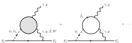
These RPV interactions are of Yukawa type, and are lepton number violating. The RPV interactions with CP phase contribute to those of the fermion EDM
| (3) |
and the quark chromo-EDM
| (4) |
from the two-loop level Barr-Zee type diagrams (see Fig. 1) susyedm2-loop ; barr-zee ; godbole ; chang ; faessler ; yamanaka1 ; rpvedmsfermion . Here the coefficients in (3) and (4) are expressed in terms of the RPV couplings as
| (5) | |||||
| (6) |
where and are defined in Eqs. (65) and (71) of Appendix A, respectively. The indices and are the generation of the inner loop and external fermions, respectively. The RPV couplings and are defined as follows: if the inner loop fermion is a lepton, if the inner loop fermion is a (down-type) quark, if is a lepton, and if is a (down-type) quark. It should be noted that, if there were the bilinear RPV interactions, the leading RPV effect would appear at the one-loop level choi ; cch .
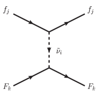
The EDM and the chromo-EDM of fermions seen above are P, CP-odd quantities generated in a straightforward way by elementary processes of a single fermion. For the case of composite systems such as hadrons, nuclei and atoms on the other hand, their EDMs are produced through the P, CP-odd four-fermion interactions. The trilinear RPV interactions (2) contribute to the P, CP-odd four-fermion interaction at the tree level as shown in Fig. 2 herczege-n ; faessler . The four-fermion interaction can be written as follows:
| (7) |
where or , depending on whether the fermion is a lepton or quark. Also, or when the fermion is a lepton or quark, respectively.
In this analysis, the sparticle mass (to be denoted generically by ) is taken to be TeV, in accordance with the exclusion region of the LHC experiment susylhc . We also assume that the flavor off-diagonal terms of the soft SUSY breaking terms are small gabbiani . We assume that the CP violation in the -parity conserving sector is minimal. The -term is removed with Peccei-Quinn symmetry peccei . In addition, we assume that the sfermion masses are degenerate. Under this condition, the contribution from the 2-loop level rainbowlike diagram vanishes yamanakarainbow1 ; yamanakarainbow2 .
II.2 Classification of the RPV contribution
As we see in Eqs. (5) and (7), fermion EDMs and CP-odd four-fermion interactions depend on imaginary parts of certain combinations of bilinear products of and/or . The combinations depend on EDM-measured objects and it will be helpful to classify the bilinear products before we start detailed analyses. With these purposes in our mind, we have classified, in the previous work yamanakabook , the RPV contributions to the EDMs into 6 types:
-
•
Type 1: Leptonic bilinears which contribute only to the electron EDM via the Barr-Zee diagram [Im() and Im()]. The EDM of paramagnetic atoms and molecules are very sensitive to them.
-
•
Type 2: Semi-leptonic bilinears involving electron which contribute both to the electron EDM and P, CP-odd electron-nucleon (e-N) interactions [Im(), Im() and Im() ()]. Atomic EDMs (paramagnetic and diamagnetic) are very sensitive to them.
-
•
Type 3: Semi-leptonic bilinears involving d-quark and heavy leptons. These can be only constrained via nucleon EDM [Im() () and Im() ()].
-
•
Type 4: Hadronic bilinears. They contribute to the d-quark EDM, choromo-EDM and P, CP-odd 4-quark interactions [Im(), Im() and Im() ()]. Purely hadronic EDMs (nucleon EDMs, bare nuclear EDMs) are highly sensitive to them.
-
•
Type 5: Bilinears which contribute only to muon EDM [Im(), Im() and Im() ()].
-
•
Type 6: Remaining RPV bilinears which cannot be constrained in this analysis [Im() and Im() ()]. They are expected to contribute to the EDMs of lepton, and quarks.
We are well aware of experiments trying to measure the muon and lepton EDM pdg , and they could provide us with stringent constraints in the near future raidal . However for now, we have not considered the Type 5 and Type 6 contributions in our analysis, which can be studied independently from the atomic and nuclear EDM’s.
II.3 P, CP-odd electron-nucleon and pion-nucleon interactions
In the present subsection, we would like to outline the derivation of the P- and CP-odd electron-nucleon and pion-nucleon interactions which are both indispensable for computation of nuclear and atomic EDMs in Section II.5.
Let us begin with the P, CP-odd electron-nucleon (e-N) interactions e-nint ; khriplovichbook ; yamanakabook described by
| (8) | |||||
These interactions originally come from the P, CP-odd electron-quark interactions with the same Lorentz structure, i.e.,
| (9) | |||||
The coefficients and are obtained by looking at the r.h.s. of Eq. (7). The coefficients , , and in (8) are extracted simply by attaching a factor of the quark content of the nucleon to the corresponding ones, i.e., , , and in Eq. (9). We are thus led to the formulae
| (10) | |||||
| (11) | |||||
| (12) |
The detail of the nucleon matrix elements will be given below. The tensor-type P, CP-odd e-N interaction of Eq. (8) does not receive the RPV contribution at the level of our discussion. It is however useful to mention it since some P, CP-odd atomic level effects can be calculated using the tensor-type P, CP-odd e-N interaction (see Section II.5).
Next let us turn to the P, CP-odd pion-nucleon interactions described effectively by
| (13) | |||||
where denotes the isospin index. The third term in Eq. (13) is of tensor-type and will not be discussed because its effect is negligibly small. The first two terms with coefficients and , respectively receive two types of contributions. One is due to the quark chromo-EDM and the other is due to P, CP-odd four-quark interactions. As to the former we do not know available lattice QCD data. In this work, we use therefore the result of the QCD sum rules qcdsumrules ; pospelovreview . The contributions of the quark chromo-EDM to and have been shown pospelovreview ; pospelov as
| (14) | |||||
| (15) |
where
| (16) | |||||
| (17) |
Here and hereafter we set belayev
| (18) | |||||
The effect of the P, CP-odd four-quark interaction to on the other hand is given by the factorization approximation pospelovreview ; yamanakabook ; 4-quark :
| (19) | |||||
where the P, CP-odd four-quark coupling has to be matched with the coefficient of Eq. (7). Here we also need the data of the scalar content of nucleon. We should note that in this paper, only the isovector P, CP-odd pion-nucleon interaction receives contribution from the P, CP-odd four-quark interactions.
We are now in a position to present the detailed quark contents in nucleons which are necessary to evaluate (10), (11) and (19) and the EDM of the composite system. The hadron level calculation, which is the integral part in the EDM predictions, has some subtleties, and we have to explain it in detail. It is most favorable that the hadronic matrix elements are given by the lattice QCD calculation yamanakabook ; bhattacharya . In our calculation, we have used the lattice QCD result for the quark scalar contents of nucleon lattice ; lattice_charm_content ; bhattacharya2 . We use the following nucleon matrix elements renormalized at GeV:
| (20) | |||||
| (21) | |||||
| (22) |
For the up and down contents, we have set the value of the nucleon sigma term
| (23) |
favored by lattice QCD studies lattice and the isovector content , also derived from the analysis of several lattice QCD results alonso ; rpvbetadecay . The strange quark content was given by the lattice QCD studies lattice ; lattice_charm_content . The quark masses that we use are pdg
| (24) | |||||
| (25) | |||||
| (26) |
The scalar density of the neutron is also necessary when we compute (10), (11) and (19). To obtain the neutron matrix elements, we simply use the isospin symmetry, i.e. (), and .
Another lattice QCD result we quote is the tensor content of the nucleon latticetensorcharge ; bhattacharya2 . The proton tensor charge is expressed in terms of the momentum and the proton spin by
| (27) |
where () is the tensor content (charge) of the proton. The tensor charge of the nucleon gives the linear coefficients of the contribution of the quark EDM to the nucleon EDM bhattacharya ; yamanakabook
| (28) |
and also the linear coefficient of the contribution of the tensor-type P, CP-odd electron-quark interaction to the P, CP-odd e-N interaction khriplovichbook [see Eq. (12)]. The lattice QCD result of the proton tensor charge is latticetensorcharge
| (29) | |||||
| (30) | |||||
| (31) |
By using the isospin symmetry, we have
| (32) | |||
| (33) | |||
| (34) |
It should be noted that the tensor charge obtained from lattice QCD is smaller than the nonrelativistic quark model predictions and , often used in the literature adler . The small values of the tensor charge is explained by the superposition of the processes in which the gluon emission and absorption of the quark flip the quark tensor charge tensorsde .
The pseudoscalar contents of nucleon have been calculated phenomenologically, as cheng ; herczege-n ; yamanakabook ; alonso
| (35) | |||||
| (36) | |||||
| (37) |
where the recent experimental data of the nucleon axial charge were used as input compass ; ucna . The large value of the pseudoscalar condensates for the light quarks is due to the pion pole contribution axialsde . For the detailed derivation, see Appendix B.
The scalar and pseudoscalar bottom contents of the nucleon can be obtained via the heavy quark expansion zhitnitsky . In this work, we use
| (38) | |||||
| (39) |
Here we also assume the isospin symmetry, i.e. and . See Appendix C for the derivation.
II.4 The chromo-EDM and the nucleon EDM
We now evaluate the chromo-EDM contribution [see Eq. (4)] to the nucleon EDM gunion . In this case again we do not have any lattice QCD results at our disposal, but there are many model calculations gunion ; chemtob ; falk ; pospelovchromoedm ; hisano ; faessler ; hisanochromoedm ; fuyuto ; yamanakabook ; chiraledm , despite the large theoretical uncertainty. As the two main ways often used to discuss the chromo-EDM contribution to the nucleon EDM, we know the chiral and QCD sum rules approaches pospelovreview . The first approach is the traditional one, which has its origin in the investigation of the observability of the -term effect peccei ; crewther ; pich ; chiraledm . There it was argued that the leading contribution of the -term to the nucleon EDM is given by the pion cloud effect. The chromo-EDM is known to contribute to the nucleon EDM in a similar way. The second approach is a more recent one, focusing on the elementary level quark-gluon processes pospelovchromoedm ; hisanochromoedm .
In this work, we consider the chiral approach to highlight physical contents of the nucleon EDM. The reason is as follows. In the phenomenological determination of the pseudoscalar contents of nucleon (35), (36), and (37), we have pointed out the importance of the pion pole contribution which gives very large matrix elements axialsde . In a similar way, it is natural to consider the Nambu-Goldstone boson contribution in this case, where the nucleon EDM is enhanced by a chiral logarithm. The result of the calculation actually yields larger coefficients than those obtained from the QCD sum rules analysis fuyuto ; yamanakabook . The recent investigations in the chiral approach are pursued by using the chiral effective theory chiraledm . In this work, we have quoted the result of Ref. fuyuto . The contribution of the quark chromo-EDM to the neutron EDM is given by
| (40) |
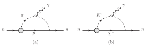
where , , and . This result was obtained by taking the leading chiral logarithm of the Nambu-Goldstone boson loop diagram as shown in Fig. 3. The Peccei-Quinn symmetry peccei was assumed, so that the quark chromo-EDM contributes also through the -term. In this derivation, the P, CP-odd pion-nucleon coupling was evaluated in the QCD sum rules.
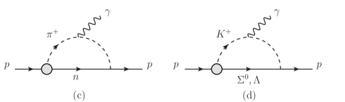
In our analysis, the expression of the proton EDM is also needed. The calculation of the proton EDM can be done in a similar way, by evaluating Fig. 4 yamanakabook . At the leading order of chiral logarithm, the convenient relations and hold. Moreover, at this order the coefficient is related to the by
| (41) |
where , and (see Appendix D for details). If we use the input parameters of Eqs. (20), (21), and (22), we obtain , so that . The coincidence of these two relations should be considered as accidental. We should note that the renormalization scale of Ref. fuyuto ( GeV) is different from that of this paper ( GeV). This difference should not be considered seriously as the theoretical uncertainty is large. If we express the proton EDM explicitly, we have
| (42) |
where , , and . The important feature of the results of the chiral approach is that the strange quark chromo-EDM contribution is not small.
In this work, we have neglected the effect of the QCD renormalization, which would give a mixing between P, CP-odd quark level operators under the change of the renormalization scale degrassi ; renormalizationedm . It should be noted in particular that the effect of the Weinberg operator weinbergoperator ; chemtob appears from the renormalization, although the RPV interactions do not generate it at the leading order. The hadron matrix elements calculated in this work however involve a large theoretical uncertainty, and the mixing effect should be well within it. We therefore neglect the renormalization of the operators together with the Weinberg operator.
II.5 Many-body physics
To determine the EDM of the nuclear and atomic level many-body systems, we need to calculate their wave functions. The leading P, CP-odd contribution used as input is the P, CP-odd pion-nucleon interactions [see Eq. (13)] and the nucleon EDM. The linear coefficients in the relation between these P, CP-odd nucleon level interactions to the nuclear EDM has to be worked out. For the calculation of the few-body systems such as the deuteron or the 3He nucleus, the ab initio approach is possible and in fact turns out to be effective liu ; gudkov ; stetcu . On the other hand, the wave functions of the systems with more than -body cannot be calculated without any approximations.
For heavy nuclei in atoms, the P, CP-odd effect is suppressed by the screening phenomenon of Schiff schiff , but the finite volume effect can generate the atomic EDM through the nuclear Schiff moment ginges . In the evaluation of the nuclear Schiff moment, we also calculate the linear coefficients between the nuclear Schiff moment and the P, CP-odd pion-nucleon interactions [see Eq. (13)] or the nucleon EDM. The general expression of the nuclear Schiff moment of the nucleus is given as
where , , and are the isoscalar, isovector, and isotensor P, CP-odd pion-nucleon couplings, respectively. The CP-even pion-nucleon coupling is given by ericson .
For the calculations of the coefficients of , and in Eq. (LABEL:eq:nuclearschiffmoment) for 129Xe nucleus, we use the result of the shell model yoshinaga1 ; yoshinaga2 . For the calculations of the nuclear Schiff moments of the 199Hg, 211Rn, and 225Ra, we use the results of the many-body calculation with mean-field approximation taking into account the deformation ban ; dobaczewski . There are currently variety of phenomenological interactions available. Calculations were made using the computer code HFODD hfodd within several models of phenomenological Skyrme interactions: SkO’ sko , SkM∗ skm , SLy4 sly4 , SV sv and SIII sv . The results for 199Hg, 211Rn, and 225Ra nuclei are shown in Table 1.
In Ref. ban , the dependence of the 199Hg and 211Rn nuclear Schiff moments on the valence neutron EDM, namely the coefficients in (LABEL:eq:nuclearschiffmoment), is given by the parameter which can be converted to owing to the formula ban
| (44) |
To obtain the coefficient of the proton EDM dependence in Eq. (LABEL:eq:nuclearschiffmoment), we have to replace the nucleon spin matrix element as in Eq. (44). The nuclear spin matrix elements will be calculated below. For the 199Hg and 211Rn nuclei, we take the average of the coefficients calculated with different phenomenological interactions ban . For the 225Ra nucleus, we take the result obtained with the SkO’ interaction, as recommended in Ref. dobaczewski . We see that the results have a large theoretical uncertainty.
| 199Hg | ||||
|---|---|---|---|---|
| SkM∗ (HFB) | 0.041 | 0.027 | 0.069 | 0.013 |
| SLy4 (HFB) | 0.013 | 0.006 | 0.024 | 0.007 |
| SLy4 (HF) | 0.013 | 0.006 | 0.022 | 0.003 |
| SV (HF) | 0.009 | 0.0001 | 0.016 | 0.002 |
| SIII (HF) | 0.012 | 0.005 | 0.016 | 0.004 |
| Average | 0.018 | 0.007 | 0.029 | 0.0058 |
| 211Rn | ||||
|---|---|---|---|---|
| SkM∗ | 0.042 | 0.028 | 0.078 | 0.015 |
| SLy4 | 0.042 | 0.018 | 0.071 | 0.016 |
| SIII | 0.034 | 0.0004 | 0.064 | 0.015 |
| Average | 0.039 | 0.0015 | 0.071 | 0.0015 |
| 225Ra | ||||
|---|---|---|---|---|
| SkM∗ | 4.7 | 21.5 | 11.0 | |
| SLy4 | 3.0 | 16.9 | 8.8 | |
| SIII | 1.0 | 7.0 | 3.9 | |
| SkO’ | 1.0 | 6.0 | 4.0 |
We also introduce the way to calculate the spin matrix elements of the valence proton and neutron and using the nuclear magnetic moment. These elements are needed to separate the CP-odd effect for the valence nucleon EDM contribution to the nuclear Schiff moment and for the pseudoscalar-type P, CP-odd e-N interaction [see Eq. (8)]. Phenomenologically, the valence nucleon is a superposition of the proton and neutron due to the configuration mixing. The mixing coefficients and can be obtained using the magnetic moment of the nucleus as follows:
| (45) |
where is the nuclear magnetic moment (in unit of the nuclear magneton). Here the matrix element is 1 for nuclei, and for nuclei. The magnetic moment of the proton is and that of the neutron is .
The final matter is the EDMs of atoms and molecules. In the atomic level evaluation of the EDM, we calculate the linear coefficients between the atomic (or molecular) EDMs and the nuclear Schiff moment, the P, CP-odd e-N interactions [see Eq. (8)] or the electron EDM.
For the paramagnetic systems such as the 205Tl, 210Fr atoms, YbF and ThO molecules, the enhancement factor of the electron EDM and the scalar-type P, CP-odd electron-nucleon interaction [see Eq. (8)] are calculated directly using the Relativistic Hartree-Fock approach flambaumtl ; flambaumfr ; flambaumybftho . The EDM of the paramagnetic atom or molecule is expressed as
| (46) |
where , , and are the proton, neutron and the total nucleon numbers of the nucleus , respectively. For the case of the paramagnetic molecule, , and are those of the biggest nucleus. The first term is the contribution of the electron EDM, with the enhancement factor , and the second term that from the scalar-type P, CP-odd e-N interactions. The effect of the P, CP-odd e-N interactions was expressed relative to the electron EDM contribution, because the experimental data of the paramagnetic systems are often written in terms of the electron EDM. In this work, we neglect the contribution of the pseudoscalar-type P, CP-odd e-N interaction and the nuclear Schiff moment for the 205Tl atoms and the YbF molecule. The theoretical uncertainty of the input parameters for the paramagnetic systems is known to be small, within few percents, and the results given by other approach kelly ; porsev ; mukherjee ; ybfkozlov ; nayak are more or less consistent.
The EDM of diamagnetic atoms has a moderate sensitivity on the electron EDM or the scalar-type P, CP-odd e-N interaction, due to the closed electron shell. It is therefore important to also consider the effect of other P, CP-odd effects such as the nuclear Schiff moment or the pseudoscalar-type P, CP-odd e-N interaction. In this work, the EDM of the diamagnetic atoms is expressed as
| (47) | |||||
where is the nuclear spin matrix element of the nucleus , which can be calculated using Eq. (45). For the diamagnetic atoms relevant in this work (129Xe, 199Hg, 211Rn, and 225Ra), the contributions from the nuclear Schiff moment, the pseudoscalar-type and the tensor-type P, CP-odd electron-nucleon interactions are calculated directly. We have quoted the results of the Relativistic Hartree-Fock approach improved with random phase approximation or configuration interaction plus many-body perturbation theory flambaumdiamagnetic . The theoretical uncertainty of the input parameters for the diamagnetic atoms is also small, and the results given by other approach lathaxerayb are almost consistent. The detail of the parameters used in this paper is presented in the formula of the Section IV.
The other contributions such as the effects of the electron EDM or the scalar-type P, CP-odd e-N interactions are derived from the approximate analytic formulae in terms of the tensor-type P, CP-odd e-N interactions flambaumformula . The contribution of the electron EDM and the scalar-type P, CP-odd e-N interaction to the EDM of diamagnetic atoms can be analytically related to the effect of the tensor-type P, CP-odd e-N interaction. The electron EDM contribution in diamagnetic atoms can be written as ginges ; flambaumformula
| (48) |
where ( is the Bohr radius), the spin of the nucleus , and the nuclear magnetic moment in unit of the nuclear magneton. The scalar-type P, CP-odd e-N interaction can be written as ginges ; flambaumformula
| (49) | |||||
The above two relations are accurate to . For the diamagnetic atom EDM, the coefficient of the tensor-type P, CP-odd e-N interaction [see Table 4] is often calculated. The atomic EDM generated from the electron EDM and the scalar-type P, CP-odd e-N interaction are, respectively,
| (50) | |||||
| (51) | |||||
III The linear programming method
In phenomenological perturbative analysis in general, we often encounter with constraint relations linear in physical observables. To derive the maximum of some value (relation) constrained by these relations, we have to solve the set of inequalities, and find the maximum in the allowed region. To do this, we can do a naive scan of the full parameter space by either dotting and checking or by either yes or no, the discretized space which is included in the regions constrained by input inequalities. However, this naive method looses efficiency when the parameter space becomes large, in particular when the dimension increases in number.
An efficient way to derive the maximum is the linear programming method. This method is based on the observation that the maximum is located at one of the corners of the multidimensional polygon made out of inequality constraints (if the solution exists). This can be understood as follows. The linear relation we want to maximize constitutes a constant gradient. Starting from somewhere in the allowed region, we follow the direction of the gradient to increase the linear relation. When we reach one of the “wall” (hyperplane) of constraint inequality, we follow then the direction of the projection of the gradient onto the wall. The dimension of the hyperplane we hit in going along the projected gradient diminishes in turn, and we arrive finally at some of the corners of the multidimensional polygonal allowed region. This is the point where the linear relation is maximized (of course if the gradient is found to be orthogonal with the final “hyperwall” we strike in going along the projected gradient, the whole hyperwall will be a degenerate solution of the problem). This is exactly the algorithm of the linear programming. The schematic picture of the 2-dimensional example is shown in Fig. 5.
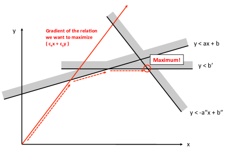
In our case, we want to predict the possible maximal value of the prepared experimental observables within the EDM-constraints. The linear inequalities and observables must be expressed by variables, which are the combination of the RPV bilinears.
IV Calculational Procedures
Let us now define all the input inequalities. We first define the relevant degrees of freedom which are the imaginary parts of the bilinear of RPV couplings. We then give the phenomenological upper bounds to the RPV couplings due to the known experimental data. We finally present the linear relations between the RPV bilinears and the CP-odd observables in questions, which are needed to yield constraints.
IV.1 RPV degrees of freedom
Let us define the set of RPV degrees of freedom in the linear programming. It is adequate to choose linearly independent combinations of RPV bilinears that appear in the relation of EDMs as our variables. The type 5 and 6 can be omitted from our analysis, since they are not related at all with the other observables. We then obtain ten variables which span the RPV parameter space relevant in our discussion. We define them as
| (52) |
These variables are the minimal set of variables linearly independent in the EDM relations (to see the relation, see Ref. yamanaka1 ). According to the classification of RPV bilinears, and belongs to the type 1. Variables , and are of the type 2, and of the type 3 and finally , and of the type 4. We must note that this decomposition has been made possible since we have assumed that the sneutrino masses (and charged slepton also) are degenerate. If this would not be the case, the combinations of RPV couplings (52) would be much more involved.
IV.2 Phenomenological constraints on RPV couplings
The above set of RPV bilinears are bounded in absolute values from other experimental data. As we are considering the full RPV parameter space which can be constrained by EDM experiments, these absolute upper limits provided by other experiments should also be taken into account. They are essentially derived from the fundamental precision test in experiments and are given in Table 2.
| RPV coupling | Upper limit | Source |
|---|---|---|
| , | Universality kao | |
| , | Universality kao | |
| , | Universality kao | |
| , | rpvkdecay ; expkdecay ; smkdecay | |
| rpvkdecay ; expkdecay ; smkdecay | ||
| Collider rpvcollider | ||
| rpvdoublebeta | ||
| mass sallydawson | ||
| decay rpvbdecay |
These limits are quite useful because the multidimensional region of the RPV coupling parameter space is now bounded by them. Thanks to these limits, we obtain the 20 linear inequalities which corresponds to a finite “box” in 10 dimensional RPV parameter space as follows:
| (53) |
All in (53) are given by assuming the SUSY masses to be equal 1 TeV. In particular, sneutrino masses are assumed to degenerate.
The P, CP-odd observables can be expressed, to the leading order in RPV bilinears, as
| (54) |
where is the label of the system (for example, He for 3He nucleus). are coefficients of the linear dependences of the P, CP-odd observable on the RPV bilinears. The EDM-constraints are then expressed in the form of inequalities
| (55) |
for Xe, Hg, Tl, YbF, ThO and . is the current experimental upper limits of the corresponding EDM observables:
| (56) |
where and are the electron EDM enhancement factors for which explicit values are not needed in this work.
IV.3 Linear coefficients of CP-odd observables
The final step of the setup is to set the inequalities due to the EDM-constraints from 129Xe, 205Tl, 199Hg atoms, YbF, ThO molecules, and neutron, and relations of the P, CP-odd observables we want to maximize (EDMs of the proton, deuteron, 3He nucleus, 211Rn, 225Ra, 210Fr atoms, muon, and the -correlation of the neutron beta decay). In this part, the scalar content of nucleon is abreviated as .
They are given as follows.
Paramagnetic atoms, molecules
Here we present the linear coefficients of the EDM of the paramagnetic atoms and molecules (205Tl, 210Fr, YbF and ThO).
| (57) | |||||
where . The atomic level parameters are given in Table 3.
| 205Tl | 582 | cm | 81 | 124 |
|---|---|---|---|---|
| 210Fr | 910 | cm | 87 | 123 |
| YbF | cm | 70 | 104 | |
| ThO | cm | 90 | 142 |
Diamagnetic atoms
The linear coefficients for the diamagnetic atoms on the other hand are given as follows:
| (58) | |||||
where . The atomic level parameters are given in Tables 4 and 5. The nuclear level parameters for the , , and nuclei are given in Table 1. For the nuclear level input parameters of the 129Xe atom, we have used the result of the shell model analysis where the nucleon spin coefficients are given by and yoshinaga1 , and the dependence of the 129Xe nuclear Schiff moment on the P, CP-odd pion-nucleon interactions is given by and yoshinaga2 .
| ( cm) | ( cm) | (cm/fm3) | |||||
|---|---|---|---|---|---|---|---|
| 129Xe | 54 | 75 | 1 | -0.7778 | |||
| 199Hg | 80 | 119 | 0.5059 | ||||
| 211Rn | 86 | 125 | 0.601 | ||||
| 225Ra | 88 | 137 | 1 | -0.734 |
| ( cm) | ||
|---|---|---|
| 129Xe | ||
| 199Hg | ||
| 211Rn | ||
| 225Ra |
Nucleon EDM
The linear coefficients for the neutron EDM are given by
| (59) |
For the proton EDM, the coefficients are obtained just by the replacement , , and in (59).
Light nuclei
The linear coefficients for the light nuclear EDM are
| (60) | |||||
where . The nuclear level parameters are given in Table 6.
-correlation
Finally the -correlation in the neutron beta decay is given simply by
| (61) |
where
| (62) |
and the ratio is given by ucna
| (63) |
| Obs. | ||||||
|---|---|---|---|---|---|---|
V Results and analysis
V.1 Constraints to RPV couplings
After performing the analysis using the linear programming method, we have found the upper limits on bilinears of RPV couplings listed in Table 9. We see that the RPV bilinears , , , , and are constrained in such a way that the limits obtained are apparently looser than those obtained in the previous analysis based on the dominance of a single RPV bilinear (see Table 10). This illustrates the large degree of freedom of the RPV supersymmetric models which accommodate much larger regions of the couplings while keeping consistency with tight EDM-constraints. Note that this analysis gives in some cases tighter upper bounds than the limits listed in Eq. (53) on the basis of other experimental sources in Table 2. We can safely say that the analysis leading to (53) gives cruder upper bounds on the RPV couplings.
| RPV bilinears | Limits () | Limits () | Limits () |
|---|---|---|---|
| 0.15 | 3.75 | 15 | |
| 0.12 | 3.0 | 12 | |
| 0.33 | 1.4 | ||
| 0.19 | 5.8 | 25 | |
| 2.6 | 14 | ||
| 2.2 | 11 | ||
| 0.38 | 2.0 | ||
| 0.76 | 3.1 | ||
| 0.15 | 3.7 | 15 |
| RPV bilinears | Limits () | Limits () | Limits () |
|---|---|---|---|
| 0.18 | 3.5 | 13 | |
| 0.26 | 0.93 | ||
V.2 Maximal prediction of the EDMs of the proton, deuteron, 3He nucleus, 211Rn, 225Ra, 210Fr atoms, and the -correlation
Next, we have made a prediction of the maximal value of the EDMs of the proton, deuteron, 3He nucleus, 211Rn, 225Ra, 210Fr atoms, and the -correlation within the linear programming method. This can be achieved by maximizing the linear relations constructed out of the coefficients of the above systems within the EDM-constraints of 205Tl, 199Hg, 129Xe, YbF, ThO, and neutron.
| Max. | |||||||
|---|---|---|---|---|---|---|---|
| 0.15 | 0.15 | 0.15 | 0.15 | 0.15 | |||
| 0.19 | 0.19 | 0.19 | 0.19 | 0.19 | |||
The obtained maximal predictions are summarized in Table 11 for . We also show the result in Table 12 obtained exactly in the same way, but with TeV. The predictions obtained here are on the same order of magnitude, since the constraints on biliears of RPV couplings given by EDMs and by other experiments (see Table 2) have similar scaling in sparticle masses.
| Max. |
|---|
Let us compare our analysis with the previous ones relying on the assumption of the dominance of one single RPV bilinear summarized in Table 10. Using these limits in Table 10, we obtain the upper limits for P, CP-odd observables as in Table 13, which are going to be inspected in next generation experiments (see also Table 14 for TeV).
| Max. |
|---|
| Max. |
|---|
We see that all predictions with the assumption of the dominance of one single RPV bilinear are well below our maximal predictions using the linear programming method, by two to four orders of magnitudes. This huge difference implies that choosing one of the couplings as the dominant one is not put on a sound basis and that there could occur conspiracy among several couplings so that the EDM constraints are satisfied. These configurations of RPV couplings have never been shed light in the previous analyses. The linear programming method shows efficiency in finding such configurations for RPV parameters. Below, we will try to explain in more detail the reasons for this large difference.
V.2.1 RPV couplings satisfying EDM-constraints of atoms and molecules
As we have argued in Chapter II.2, the atoms and molecules have a strong sensitivity to the type 2 ( and ) semi-leptonic RPV bilinears. Let us see how the RPV bilinears arrange themselves and become large consistently with the EDM-constraints. The EDM of the paramagnetic systems (205Tl atom, YbF, and ThO molecules) are sensitive to the type 2 RPV bilinears, and also to the type 1 leptonic RPV bilinears ( and ). Thus, to be consistent with the constraint provided by the paramagnetic systems, it suffices to cancel the type 1 and type 2 contributions mutually. As we can see, this is exactly what is happening in Table 11.
The constraints from the EDM of diamagnetic atoms (199Hg and 129Xe) also have strong sensitivity to type 2 RPV bilinears, since it is generated by P, CP-odd e-N interactions. Diamagnetic atoms have, however, a moderate sensitivity to type 1 bilinears. They also receive contribution from type 4 ( and ). To be consistent with experimental upper bounds, we have to cancel the type 2 and type 4 contributions. The large cancellation occurs among and . The remaining small part is cancelled with the type 4 RPV components originating in the nuclear Schiff moment. Within the above constraints, it is possible to enlarge the (=) component up to . The coefficients of the EDM of diamagnetic atoms for type 2 RPV bilinears are aligned. This explains the relatively small maximal prediction for the EDM of 211Rn atom. The same analysis does not hold for the 225Ra atom, since the EDM of 225Ra has strong sensitivity on the hadronic sector (type 4). The above inspection means that even by introducing the future experimental constraints from 211Rn and 225Ra atoms, which will be explained in Sec. V.3, it is not possible to give tight upper bounds on RPV bilinears of type 2. To rule out the type 2 bilinears, we need another observable with coefficients and not aligned with those of the diamagnetic atoms. This is possible when we use the -correlation of the neutron beta decay, which will be discussed later.
V.2.2 Limits to type 3
Throughout this analysis, the type 3 RPV bilinears are supposed to take the same value (, ). This is simply because the type 3 cannot be constrained from the linear programming analysis due to the suppression of the quark EDM by the electromagnetic coupling constant in the Barr-Zee type contribution. The limits coming from other experiments are therefore dominant in this case.
V.2.3 Hadronic observables
The purely hadronic observables (such as EDMs of the neutron, proton, deuteron and 3He nucleus) have a large sensitivity against hadronic P, CP violating RPV interactions (type 4). This is due to the absence of the screening electrons and also to the large sensitivity of the near-future experiments with novel techniques using the storage ring storage . The absence of the electrons also suppresses the semi-leptonic contribution, so that it serves to probe a fixed region of the RPV parameter space. One of the important characteristics of the purely hadronic EDMs is that they depend approximately only on type 4 RPV bilinears (type 3 contribution is relatively small). As they have restricted sensitivity against RPV bilinears, they can be used as a good probe to rule out a specific region of the RPV parameter space. This also means that accumulating the EDM experimental data of pure hadronic EDMs is an efficient way to constrain the RPV parameter space, since they receive no cancellation from other sector than type 4 RPV bilinears. We must note that the prediction of the hadronic EDMs suffers from large theoretical uncertainty due to the use of model calculations at the hadronic level, and we would not be quite sure even of the order of magnitude. To do a quantitative analysis, we must improve the accuracy of the QCD level calculation.
V.2.4 -correlation
With the assumption of the single coupling dominance, one might perhaps argue that the -correlation is not particularly useful due to the strong constraint of the atomic EDMs against CP violation. For example, within the dominance of one single bilinear of RPV couplings, the EDM of 199Hg atom can constrain the same combination Im up to with the current experimental data, whereas the -correlation can constrain only up to in the current experimental prospect of the 8Li murata , well below the EDM experimental sensitivity. The result of our analysis, however, shows the potential importance of this observable. By virtue of the fact that the -correlation depends only on one combination (at least at the tree level), it can be “safely” large without conflicting with EDM observables which depend on several couplings. The -correlation is an important probe of the absolute size of Im(). We have seen that Im() is the most sensitive RPV bilinear for the atomic EDMs, and combined with the EDM-constraints of paramagnetic and diamagnetic atoms, we can fully constrain the type 2 RPV bilinears. If the -correlation can be measured with sufficient accuracy, it is possible to rule out the large prediction of atomic EDMs from Im(), thus reducing a large portion of the contribution to them. The experimental development in searching for the -correlation should therefore be strongly urged.
V.2.5 Muon EDM
The muon EDM is out of the scope of the present paper, but this observable sits in a special position, so we should add some comment. The muon EDM depends on Im, Im, and Im via the two-loop level Barr-Zee type diagram, but these combinations do not contribute to the other available P, CP-odd observables. In RPV, the muon EDM is actually completely independent of other observables and can constrain its own RPV parameter space exclusively. As we do not have any other resource of EDM experimental data which can constrain the RPV couplings under consideration, the maximal prediction is just the sum of the upper bounds of RPV bilinears which can be probed with the muon EDM, and is of order . The present experimental sensitivity ( muong2 ) is well below the existing limits to the RPV couplings from other experiments. The future muon EDM experiments is prepared to aim at the order of storage , but the maximal value predicted in this analysis is also of the same order. Thus it will be difficult to either probe or constrain these RPV bilinears.
V.2.6 Theoretical uncertainties
Let us briefly mention theoretical uncertainties of this analysis. The first source of large theoretical uncertainty is the nuclear level calculations. The actual results of the Schiff moment calculations are not always consistent with each other (see Table 1). We have tested the dependence of the linear programming analysis on the different results presented in Ref. ban . The results may vary by one or two orders of magnitude. This illustrates the large uncertainty due to the nuclear level calculation of the Schiff moments of nuclei with deformation. The reduction of the theoretical uncertainty associated with odd numbered nuclei with deformation is one of the problems that challenges us.
The second large theoretical uncertainty comes from the hadron level calculation. To derive the hadronic contribution of the chromo-EDM operator, we have used the chiral techniques, which have a strong dependence on the cutoff scale hisano ; fuyuto and are not considered to be accurate better than 100%. In the hadron sector, the final result may also change by an order of magnitude. To reduce these theoretical uncertainties, the lattice QCD study is absolutely needed bhattacharya .
By considering these sources of theoretical error, we have to say that coefficients , , , and could differ by an order of magnitude.
V.2.7 Improvement of constraints on RPV couplings from other experiments
We must note that the limits on RPV couplings can be tightened possibly by improving the constraints provided by other experiments in the linear programming analysis. This is because the reductions of the allowed region of the (absolute values of) RPV couplings can be expected to constrain the degrees of freedom left for the rearrangement of parameters within (EDM-)constraints. Here we mention the possible potentiality of other experiments.
The first possibility is to improve the experimental accuracy of the measurements of lepton decays (universality test) and hadron decays (, ) (see Table 2).
The second possibility is the constraint from the absolute mass of neutrinos. All lepton number violating RPV interactions contribute to the Majorana mass of the neutrinos, so the improvement of experimental constraints on their masses has a large potential to limit RPV bilinears relevant in our analysis.
The third interesting possibility is the limit to be afforded by collider experiments. Actually, resonances of sneutrino arise in the presence of the RPV interactions at collider experiments rpvcollider . The parton distributions for strange and bottom quarks also allow to probe the RPV interactions and . The lepton collider is sensitive to the resonances of sneutrino generated by leptonic RPV interactions (electron collision), (muon collision) and ( lepton collision).
V.3 Prospective upper limits of EDMs
Finaly we would like to supplement a rather peripheral analyses. Namely we add an estimate of the constraints on RPV bilinears when the prospective upper limits of the EDMs of 129Xe, neutron, proton, deuteron, 3He nucleus, 211Rn, 225Ra, and 210Fr atoms are imposed. We will set the following limits, regarding the prospects of the experimental sensitivity storage ; bnl ; mueller ; sakemi ; ucn ; xeasahi :
| (64) |
Let us first see the limits on RPV bilinears with a combined use of (64) and the linear programming method for the six EDM-constraints (205Tl, 199Hg, 129Xe, YbF, ThO and neutron) seen previously. The result is shown in Table 15.
| RPV bilinear | All | ||||||||
|---|---|---|---|---|---|---|---|---|---|
| 0.15 | 0.15 | 0.15 | 0.15 | 0.15 | 0.15 | 0.15 | 0.15 | 0.15 | |
| 0.12 | 0.12 | ||||||||
| 0.19 | 0.10 | 0.19 | |||||||
| 0.15 | 0.15 | 0.15 | 0.15 |
By comparing Tables 9 and 15, we see that many RPV bilinears (, , , , , , and ) can further be constrained by considering experimental data that are expected to come in the future. This result shows the importance of the prospective experiments. The following observations can be done:
-
•
RPV bilinears and cannot be constrained at all. This is due to the small contribution of the Barr-Zee type diagram with the second generation fermion in the inner loop (the Barr-Zee type diagram is sensitive to the inner loop fermion mass).
-
•
The expected bound on the proton EDM in (64) is only effective for limiting , in spite of the strong dependence of the proton EDM on the purely hadronic bilinears (type 4). This is due to the alignment of the coefficients with the neutron EDM.
-
•
By taking into account of the EDM-constraints of the deuteron, 3He nucleus and 225Ra atom in (64), the hadronic RPV bilinears and are constrained by two orders of magnitude tighter. This shows the strong sensitivity of hadronic EDMs (deuteron and 3He) against and . The EDM of 225Ra atom is also sensitive to the hadronic -parity violation, due to the strong enhancement of the nuclear Schiff moment.
-
•
The leptonic and semi-leptonic RPV bilinears , and , although moderate, can be constrained with any additional prospective EDM constraints. Naïvely, this fact is not obvious, since the purely hadronic EDMs ( and ) are not sensitive to , and . This can be understood by the interplay between the additional future EDM-constraints and the existing constraints of diamagnetic atoms (199Hg and 129Xe). This fact shows the importance of considering as many systems of the experimental EDM-constraints as possible.
-
•
The experimental limit of the 211Rn EDM can give tighter constraints on , , , and . This is realized thanks to the strong (prospective) EDM-constraints.
-
•
As we see from Tables 9 and 15, improved measurements of neutron EDM will not necessarily provide us with more precise information of ’s. This is simply explained by the fact that the location of the maximum point in the parameter space is away from the hyperplane determined by the constraints of the neutron dipole moment.
We have also given upper limits when all prospective EDM-constraints are applied simultaneously, and the result gives very strong limits on RPV couplings. We understand that, when the number of constraints exceeds the number of the RPV bilinears, these strong limitations often occur. It is to be noted that by considering all prospective limits, we can constrain the RPV bilinear . We can conclude from these results that the combination of many EDM-constraints are useful in setting upper bounds on the RPV interactions.
VI Conclusion
In summary, we have done an extensive analysis having a careful look at every corner of the full CP violating RPV parameter space. We have developed a new calculational technique based on the linear programming method, have given limits on the imaginary parts of RPV bilinears, and have predicted the maximally possible values for observables of prepared or on-going experiments (proton, deuteron, 3He nucleus, 211Rn, 225Ra, 210Fr atoms, muon, and the -correlation of the neutron beta decay) under the currently available experimental constraints (56) (in addition to other CP conserving experimental data of fundamental precision tests listed in Table 2). We have found through this analysis that the RPV bilinears , , , and can be constrained by the current available experimental EDM-constraints.
The upper limits for ’s obtained by linear programming method differ from those obtained under the hypothesis of the single-coupling dominance by a few orders of magnitudes. The larger upper limits in the linear programing method has been made possible because of the destructive interference among the terms in Eq. (54), thereby we have looked for the maximum parameter space of within the constrains of EDM data. On the other hand, destructive cancellation in Eq. (54) was avoided as much as possible when we looked for maximally possible values of EDMs of proton, deuteron, He, Rn, Ra, and Fr in Table 11 and Table 12. Only for the EDM of proton and Fr, the cancellation is of two and one digits respectively.
When we look at the numbers of in Table 11, we notice that is much smaller than other ’s. This means that among the two terms in the sum large cancellation could admittedly be occurring.
The upper limits on the above-mentioned RPV-bilinears , , , , and together with , , and can be tightened with additional prospective EDM-constraints of the proton, deuteron, 3He nucleus, 211Rn and 225Ra atoms given in (64). In particular, and can be strongly constrained due to the high sensitivity of the planned EDM experiments. RPV bilinears and have not yet been constrained due to the rather poor sensitivity of the EDMs of the relevant systems.
For the prediction of prospective experiments, we have found that very large values are still allowed. This result is encouraging for experimentalists, since there is still a possibility to observe large EDM for prospective experiments. We have made a comparison of our analyses with the “classic” ones which assume the dominance of only one or a few combinations of couplings among several others. We have demonstrated the potential importance of the regions in the parameter space which had never been given due consideration. As it has turned out in this work, intriguing observables are the -correlation, the purely hadronic EDMs and the muon EDM which have sensitivity to the restricted area of the RPV parameter space. We have also obtained the useful information that the -correlation is an important probe to rule out the type 2 RPV bilinears. Although we believe that applications of linear programming method in this work is quite successful, we have to admit some troubles due to the theoretical uncertainties. The reduction of them, in particular at the hadronic and nuclear level, are urgently required.
Finally we would like to mention a subject which is left open for our future work. In the present work, we have analyzed the EDM-constraints as linear relations in the linear programming, but the absolute limits on the RPV couplings taken from other experimental data were assumed to hold only for a single RPV coupling. As a future subject, we have to treat also these absolute limits offered by other experiments as linear relation inputs in the analysis of linear programming.
Acknowledgements.
The authors thank T. Hatsuda for useful discussion and comments. This work is in part supported by the Grant for Scientific Research [Priority Areas “New Hadrons” (E01:21105006), (C) No.23540306] from the Ministry of Education, Culture, Science and Technology (MEXT) of Japan and JSPS KAKENHI Grant No. 24540273 and 25105010(T.S.). This is also supported by the RIKEN iTHES Project.Appendix A Barr-Zee type contribution to the fermion EDM and quark chromo-EDM
The contribution to the EDM of a fermion due to the photon exchange RPV Barr-Zee type graph (see Fig. 1) is given by rpvedmsfermion
| (65) | |||||
where and are respectively the flavor index and the electric charge in unit of of the external fermion . Likewise and are respectively the flavor index and electric charge in unit of of the the inner loop fermion (or sfermion ). In the left-hand side of (65), , , and are the Barr-Zee type contributions with photon, and boson exchange, respectively, to be defined below. Note that the electric charge is positively defined, in contrast to Refs. yamanakabook ; yamanaka1 ; rpvedmsfermion .
The photon exchange RPV effect is
| (66) | |||||
where is the color number of the inner loop fermion or sfermion ( if inner loop fermion is a quark, otherwise ). The mass of the exchanged sneutrino is given by . The function is defined as
| (67) | |||||
The last approximation holds for small . Note that the Barr-Zee type diagram gives EDM contribution only to down-type quarks (the same property holds also for the chromo-EDM seen below).
The contribution to the EDM of the fermion from the boson exchange RPV Barr-Zee type graph is given by rpvedmsfermion
where the weak coupling for being a charged lepton, and for being a down-type quarks. For the sfermion weak coupling, we have and , where for being a charged lepton or down-type quark. The integral is defined as
| (69) | |||||
The exchange RPV Barr-Zee diagram contribution turns out to be rpvedmsfermion
where is the Cabibbo-Kobayashi-Maskawa matrix element, and denote the down- and up-type inner loop fermions, respectively. The mass of the selectron is denoted by . Here we have again used the integral of Eq. (69).
The Barr-Zee type graph contribution to the down-type quark chromo-EDM is
| (71) | |||||
where and are again the flavor indices of the quark and the fermion of the inner loop, respectively.
Appendix B Phenomenological pseudoscalar contents of nucleon
The derivation of the pseudoscalar condensates goes along the line of Ref. cheng . The anomalous Ward identity requires
| (72) | |||||
| (73) | |||||
| (74) |
where , , and compass . The anomaly contribution is defined as , and is given by
| (75) | |||||
where compass , and . Here is the correction to the Goldberger-Treiman relation, where we have used ericson . By equating the above equations, we obtain Eqs. (35), (36), and (37).
Appendix C Heavy quark contents of nucleon
Here we calculate the heavy quark content of the nucleon. The scalar content of nucleon satisfies the following relation
| (76) |
where with . The first term on the right hand side of (76) is the contribution in the chiral limit, and the other terms the finite quark mass contribution to the nucleon mass. In the heavy quark expansion, the scalar heavy quark condensates are given by zhitnitsky
| (77) |
where . By equating Eqs. (76) and (77), we obtain (renormalization scale GeV)
| (78) | |||||
| (79) | |||||
| (80) | |||||
| (81) |
where we have used the result of the lattice QCD study of the nucleon sigma term MeV lattice , and numerical values (20) - (22) input parameters. The result of the charm quark content is to be compared with the recent lattice QCD result lattice_charm_content , which is on the same order of magnitude.
The pseudoscalar heavy quark contents of nucleon can be written in the leading order of the heavy quark expansion zhitnitsky as
| (82) | |||||
By using Eq. (75), we obtain
| (83) | |||||
| (84) | |||||
| (85) |
Appendix D Quark chromo-EDM contribution to the nucleon EDM
The leading contribution of the quark chromo-EDM to the neutron and proton EDMs is given by the chiral logarithm of the meson-loop diagrams shown in Figs. 3 and 4. The dependence of the nucleon EDMs on the quark chromo-EDM is given by hisano ; fuyuto ; yamanakabook
| (86) | |||||
with
where , , , , and . By assuming , we find Eq. (41).
Appendix E RPV contribution to the -correlation
We briefly present the -correlation of the neutron beta decay, a powerful probe of the new physics with the small SM background betadecaybeyondsm ; ckmbetadecay . This observable, like the EDMs, is also sensitive to the P and CP violations of the underlying theory. The angular distribution of the neutron beta decay can be written as jacksontreiman
| (88) |
where -correlation is the last term, the triple product of the initial neutron polarization, emitted electron polarization and momentum. This observable is odd under P and CP.
The tree level RPV contribution to the -correlation of the neutron beta decay is given by the diagram given in Fig. 6.
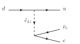
The nucleon level effective interaction is then
| (89) |
where has been obtained by taking the isospin breaking to the first order alonso ; rpvbetadecay . The lattice QCD study of also gives a consistent result bhattacharya2 . We finally obtain the -correlation formula presented previously in (61) and (62)
| (90) |
where is given by (63). One of the important characteristics of the -correlation relevant in this discussion is that it depends only on the RPV combinations Im().
References
- (1) H. E. Haber and G. L. Kane, Phys. Rep. 117, 75 (1985); J. F. Gunion and H. E. Haber, Nucl. Phys. B 272, 1 (1986); S. P. Martin, in Perspectives on Supersymmetry II, edited by G. L. Kane (World Scientific, Singapore, 2010), p. 1 [arXiv:hep-ph/9709356].
- (2) G. Bhattacharyya, arXiv:hep-ph/9709395; H. K. Dreiner, in Perspectives on Supersymmetry II, edited by G. L. Kane (World Scientific, Singapore, 1997), p. 565 [arXiv:hep-ph/9707435]; M. Chemtob, Prog. Part. Nucl. Phys. 54, 71 (2005); R. Barbier et al., Phys. Rep. 420, 1 (2005); H. K. Dreiner, M. Kramer, and B. O’Leary, Phys. Rev. D 75, 114016 (2007); Y. Kao and T. Takeuchi, arXiv:0910.4980 [hep-ph]; H. K. Dreiner, K. Nickel, F. Staub, and A. Vicente, Phys. Rev. D 86, 015003 (2012).
- (3) X.-G. He, B. H. J. McKellar, and S. Pakvasa, Int. J. Mod. Phys. A 4, 5011 (1989) [Erratum-ibid. A 6, 1063 (1991)]; W. Bernreuther and M. Suzuki, Rev. Mod. Phys. 63, 313 (1991); T. Fukuyama, Int. J. Mod. Phys. A 27, 1230015 (2012); O. Naviliat-Cuncic and R. G. E. Timmermans, Comptes Rendus Physique 13, 168 (2012); J. Engel, M. J. Ramsey-Musolf, and U. van Kolck, Prog. Part. Nucl. Phys. 71, 21 (2013); K. Jungmann, Ann. Phys. (Berlin) 525, 550 (2013).
- (4) I. B. Khriplovich and S. K. Lamoreaux, CP Vioaltion Without Strangeness, Springer, Berlin (1997).
- (5) M. Pospelov and A. Ritz, Ann. Phys. 318, 119 (2005).
- (6) J. S. M. Ginges and V. V. Flambaum, Phys. Rep. 397, 63 (2004).
- (7) N. Yamanaka, “Analysis of the Electric Dipole Moment in the R-parity Violating Supersymmetric Standard Model”, Springer, Berlin, Germany (2014).
- (8) M. A. Rosenberry and T. E. Chupp, Phys. Rev. Lett. 86, 22 (2001).
- (9) B. C. Regan, ,E. D. Commins, C. J. Schmidt, and D. DeMille, Phys. Rev. Lett. 88, 071805 (2002).
- (10) C. A. Baker et al., Phys. Rev. Lett. 97, 131801 (2006).
- (11) W. C. Griffith, M. D. Swallows, T. H. Loftus, M. V. Romalis, B. R. Heckel, and E. N. Fortson, Phys. Rev. Lett. 102, 101601 (2009).
- (12) G. W. Bennett et al. (Muon () Collaboration), Phys. Rev. D 80, 052008 (2009).
- (13) J. J. Hudson, D. M. Kara, I. J. Smallman, B. E. Sauer, M. R. Tarbutt, and E. A. Hinds, Nature (London) 473, 493 (2011); New J. Phys. 14, 103051 (2012).
- (14) J. Baron et al. (ACME Collaboration), Science, (2013); arXiv:1310.7534 [physics.atom-ph].
- (15) Storage Ring EDM Collaboration, http://www.bnl.gov/edm/.
- (16) I. B. Khriplovich, Phys. Lett. B 444, 98 (1998); F. J. M. Farley et al., Phys. Rev. Lett. 93, 052001 (2004); Y. K. Semertzidis et al., AIP Conf. Proc. 698, 200 (2004); Y. F. Orlov, W. M. Morse, and Y. K. Semertzidis, Phys. Rev. Lett. 96, 214802 (2006).
- (17) P. Mueller et al., Talk given at the 5th International conference on ”Fundamental Physics Using Atoms”, Okayama (October, 2011).
- (18) H. Abele, Prog. Part. Nucl. Phys. 60, 1 (2008); D. Dubbers and M. G. Schmidt, Rev. Mod. Phys. 83, 1111 (2011); J.W. Martin et al., Talk given at the 5th International conference on ”Fundamental Physics Using Atoms”, Okayama (October, 2011).
- (19) A. Yoshimi et al., Phys. Lett. A 376, 1924 (2012).
- (20) Y. Sakemi et al., J. Phys. Conf. Ser. 302, 012051 (2011).
- (21) J. R. Ellis, M. K. Gaillard, and D. V. Nanopoulos, Nucl. Phys. B 109, 213 (1976); E. P. Shabalin, Yad. Fiz. 28, 151 (1978) [Sov. J. Nucl. Phys. 28, 75 (1978)]; Yad. Fiz. 31, 1665 (1980) [Sov. J. Nucl. Phys. 31, 864 (1980)]; Yad. Fiz. 32, 443 (1980) [Sov. J. Nucl. Phys. 32, 228 (1980)]; J. Ellis and M. K. Gaillard, Nucl. Phys. B 150, 141 (1979); D. V. Nanopoulos, A. Yildiz, and P. H. Cox, Phys. Lett. B 87, 53 (1979); M. B. Gavela, A. Le Yaouanc, L. Oliver, O. Pène, J.-C. Raynal, and T. N. Pham, Phys. Lett. B 109, 215 (1982); N. G. Deshpande, G. Eilam, and W. L. Spence, Phys. Lett. B 108, 42 (1982); I. B. Khriplovich and A. R. Zhitnitsky, Phys. Lett. B 109, 490 (1982); J. O. Eeg and I. Picek, Nucl. Phys. B 244, 77 (1984); C. Hamzaoui, and A. Barroso, Phys. Lett. B 154, 202 (1985); I. B. Khriplovich, Yad. Fiz. 44, 1019 (1986) [Sov. J. Nucl. Phys. 44, 659 (1986)]; Phys. Lett. B 173, 193 (1986); J. F. Donoghue, B. R. Holstein, and M. J. Musolf, Phys. Lett. B 196, 196 (1987); M. E. Pospelov and I. B. Khriplovich, Yad. Fiz. 53, 1030 (1991) [Sov. J. Nucl. Phys. 53, 638 (1991)]; X.-G. He and B. McKellar, Phys. Rev. D 46, 2131 (1992); X.-G. He, B. H. J. McKellar, and S. Pakvasa, Phys. Lett. B 283, 348 (1992); M. J. Booth, arXiv:hep-ph/9301293; Phys. Rev. D 48, 1248 (1993); M. E. Pospelov, Phys. Let. B 328, 441 (1994); A. Czarnecki and B. Krause, Phys. Rev. Lett. 78, 4339 (1997); S. Dar, arXiv:hep-ph/0008248; T. Mannel and N. Uraltsev, Phys. Rev. D 85, 096002 (2012).
- (22) J. R. Ellis, S. Ferrera, and D. V. Nanopoulos, Phys. Lett. B 114, 231 (1982); W. Buchmüller and D. Wyler, Phys. Lett. B 121, 321 (1983); J. Polchinski and M. B. Wise, Phys. Lett. B 125, 393 (1983); F. del Aguila, M. B. Gavela, J. A. Grifols, and A. Mendez, Phys. Lett. B 126, 71 (1983); D. V. Nanopoulos and M. Srednicki, Phys. Lett. B 128, 61 (1983); M. Dugan, B. Grinstein, and L. J. Hall, Nucl. Phys. B 255, 413 (1985); P. Nath, Phys. Rev. Lett. 66, 2565 (1991); Y. Kizukuri and N. Oshimo, Phys. Rev. D 45, 1806 (1992); Phys. Rev. D 46, 3025 (1992); W. Fischler, S. Paban, and S. D. Thomas, Phys. Lett. B 289, 373 (1992); T. Inui, Y. Mimura, N. Sakai, and T. Sasaki, Nucl. Phys. B 449, 49 (1995); T. Ibrahim and P. Nath, Phys. Rev. D 57, 478 (1998); Phys. Lett. B 418, 98 (1998); Phys. Rev. D 58, 111301 (1998); S. Pokorski, J. Rosiek, and C. A. Savoy, Nucl. Phys. B 570, 81 (2000); S. Y. Ayazi and Y. Farzan, Phys. Rev. D 74, 055008 (2006); J. High Energy Phys. 06 (2007), 013.
- (23) T. H. West, Phys. Rev. D 50, 7025 (1994); T. Kadoyoshi and N. Oshimo, Phys. Rev. D 55, 1481 (1997); D. Chang, W.-Y. Keung, and A. Pilaftsis, Phys. Rev. Lett. 82, 900 (1999); A. Pilaftsis, Phys. Lett. B 471, 174 (1999); D. Chang, W.-F. Chang, and W.-Y. Keung, Phys. Lett. B 478, 239 (2000); A. Pilaftsis, Phys. Rev. D 62, 016007 (2000); D. Chang, W.-F. Chang, and W.-Y. Keung, Phys. Rev. D 66, 116008 (2002); T.-F. Feng, X.-Q. Li, J. Maalampi, and X. Zhang, Phys. Rev. D 71, 056005 (2005); N. Arkani-Hamed, S. Dimopoulos, G.F. Giudice, and A. Romanino, Nucl. Phys. B 709, 3 (2005); D. Chang, W.-F. Chang, and W.-Y. Keung, Phys. Rev. D 71, 076006 (2005); G. F. Giudice and A. Romanino, Phys. Lett. B 634, 307 (2006); T.-F. Feng, X.-Q. Li, L. Lin, J. Maalampi, and H.-S. Song, Phys. Rev. D 73, 116001 (2006); Y. Li, S. Profumo, and M. J. Ramsey-Musolf, Phys. Rev. D 78, 075009 (2008).
- (24) N. Yamanaka, Phys. Rev. D 87, 011701 (2013).
- (25) J. Dai, H. Dykstra, R. G. Leigh, S. Paban, and D. Dicus, Phys. Lett. B 237, 216 (1990); M. Brhlik, G. J. Good, and G. L. Kane, Phys. Rev. D 59, 115004 (1999); S. Abel, S. Khalil, and O. Lebedev, Nucl. Phys. B 606, 151 (2001); A. Pilaftsis, Nucl. Phys. B 644, 263 (2002); O. Lebedev and M. Pospelov, Phys. Rev. Lett. 89, 101801 (2002); D. Demir, O. Lebedev, K. A. Olive, M. Pospelov, and A. Ritz, Nucl. Phys. B 680, 339 (2004); O. Lebedev, K. A. Olive, M. Pospelov, and A. Ritz, Phys. Rev. D 70, 016003 (2004); K. A. Olive, M. Pospelov, A. Ritz, and Y. Santoso, Phys. Rev. D 72, 075001 (2005); S. Abel and O. Lebedev, J. High Energy Phys. 01, 133 (2006); J. Ellis, J. S. Lee, and A. Pilaftsis, J. High Energy Phys. 10, 049 (2008); Y. Li, S. Profumo, and M. J. Ramsey-Musolf, J. High Energy Phys. 08, 062 (2010); K. Fuyuto, J. Hisano, N. Nagata, and K. Tsumura, J. High Eenergy Phys. 1312, 010 (2013); S. A. R. Ellis and G. L. Kane, arXiv:1405.7719 [hep-ph].
- (26) T. Falk, K. A. Olive, M. Pospelov, and R. Roiban, Nucl. Phys. B 560, 3 (1999).
- (27) J. Hisano and Y. Shimizu, Phys. Rev. D 70, 093001 (2004).
- (28) G. Degrassi, E. Franco, S. Marchetti, and L. Silvestrini, J. High Energy Phys. 11, 044 (2005).
- (29) J. Hisano and Y. Shimizu, Phys. Lett. B 581, 224 (2004); M. Endo, M. Kakizaki, and M. Yamaguchi, Phys. Lett. B 583, 186 (2004); G.-C. Cho, N. Haba, and M. Honda, Mod. Phys. Lett. A 20, 2969 (2005); J. Hisano, M. Nagai, and P. Paradisi, Phys. Lett. B 642, 510 (2006); Phys. Rev. D 78, 075019 (2008); Phys. Rev. D 80, 095014 (2009); W. Altmannshofer, A. J. Buras, and P. Paradisi, Phys. Lett. B 688, 202 (2010).
- (30) J. Ellis, J. S. Lee, and A. Pilaftsis, J. High Energy Phys. 10, 049 (2010); J. High Energy Phys. 02, 045 (2011); arXiv:1009.1151 [math.OC].
- (31) W. Dekens, J. de Vries, J. Bsaisou, W. Bernreuther, C. Hanhart, U.-G. Meißner, A. Nogga, and A. Wirzba, arXiv:1404.6082 [hep-ph].
- (32) R. Barbieri and A. Masiero, Nucl. Phys. B 267, 679 (1986).
- (33) R. M. Godbole, S. Pakvasa, S. D. Rindani, and X. Tata, Phys. Rev. D 61, 113003 (2000); S. A. Abel, A. Dedes, and H. K. Dreiner, JHEP05, 13 (2000).
- (34) D. Chang, W.-F. Chang, M. Frank, and W.-Y. Keung, Phys. Rev. D 62, 095002 (2000).
- (35) P. Herczeg, Phys. Rev. D 61, 095010 (2000); N. Yamanaka, Phys. Rev. D 85, 115012 (2012).
- (36) Y. Y. Keum and Otto C. W. Kong, Phys. Rev. Lett. 86, 393 (2001); Phys. Rev. D 63, 113012 (2001); C.-C. Chiou, O. C. W. Kong, and R. D. Vaidya, Phys. Rev. D 76, 013003 (2007).
- (37) K. Choi, E. J. Chun, and K. Hwang, Phys. Rev. D 63, 013002 (2000).
- (38) A. Faessler, T. Gutsche, S. Kovalenko, and V. E. Lyubovitskij, Phys. Rev. D 73, 114023 (2006); Phys. Rev. D 74, 074013 (2006).
- (39) N. Yamanaka, T. Sato, and T. Kubota, Phys. Rev. D 85, 117701 (2012); N. Yamanaka, Phys. Rev. D 86, 075029 (2012).
- (40) N. Yamanaka, T. Sato, and T. Kubota, Phys. Rev. D 87, 115011 (2013).
- (41) J. Ellis, G. Gelmini, C. Jarlskog, G. G. Ross, and J. W. F. Valle, Phys. Lett. B 150, 142 (1985); M. Bisset, O. C. W. Kong, C. Macesanu, and L. H. Orr, Phys. Lett. B 430, 274 (1998); O. C. W. Kong, Int. J. Mod. Phys. A 19, 1863 (2004).
- (42) S. Dawson, Nucl. Phys. B 261, 297 (1985).
- (43) S. M. Barr and A. Zee, Phys. Rev. Lett. 65, 21 (1990); R. G. Leigh, S. Paban, and R.-M. Xu, Nucl. Phys. B 352, 45 (1991); D. Chang, W.-Y. Keung, and J. Liu, Nucl. Phys. B 355, 295 (1991); D. Chang, W.-Y. Keung, and T. C. Yuan, Phys. Rev. D 43, R14 (1991); C. Kao and R.-M. Xu, Phys. Lett. B 296, 435 (1992); V. Barger, A. Das, and C. Kao, Phys. Rev. D 55, 7099 (1997); D. Bowser-Chao, D. Chang, and W.-Y. Keung, Phys. Rev. Lett. 79, 1988 (1997); A. J. Buras, G. Isidori, and P. Paradisi, Phys. Lett. B 694, 402 (2011); T. Abe, J. Hisano, T. Kitahara, and K. Tobioka, J. High Energy Phys. 1401, 106 (2014); S. Inoue, M. J. Ramsey-Musolf, and Y. Zhang, arXiv:1403.4257 [hep-ph]; K. Cheung, J. S. Lee, E. Senaha, and P.-Y. Tseng, arXiv:1403.4775 [hep-ph].
- (44) ATLAS Collaboration (Georges Aad et al.), Phys. Rev. Lett. 106, 131802 (2011); Phys. Lett. B 701, 186 (2011); Phys. Lett. B 703, 428 (2011); Phys. Lett. B 709, 137 (2012); ATLAS Collaboration, ATLAS-CONF-2013-024; ATLAS Collaboration, ATLAS-CONF-2013-035; CMS Collaboration (Vardan Khachatryan et al.), Phys. Lett. B 698, 196 (2011);. CMS Collaboration (S. Chatrchyan et al.), Phys. Lett. B 722, 273 (2013); Phys. Lett. B 725, 243 (2013).
- (45) F. Gabbiani, E. Gabrielli, A. Masiero, and L. Silvestrini, Nucl. Phys. B 477, 321 (1996).
- (46) R. D. Peccei and H. R. Quinn, Phys. Rev. Lett. 38, 1440 (1977).
- (47) Similar diagrams contributing to the muon was calculated in H. Fargnoli, C. Gnendiger, S. Passehr, D. Stöckinger, and H. Stöckinger-Kim, J. High Energy Phys. 1402 (2014) 070.
- (48) K.A. Olive et al. (Particle Data Group), Chin. Phys. C 38, 090001 (2014).
- (49) M. Raidal et al., Eur. Phys. J. C 57, 13 (2008).
- (50) S. M. Barr, Phys. Rev. D 45, 4148 (1992).
- (51) M. A. Shifman, A. I. Vainshtein, and V. I. Zakharov, Nucl. Phys. B 147, 385 (1979); B 147, 448 (1979); B 147, 519 (1979); P. Colangelo and A. Khodjamirian, arXiv:hep-ph/0010175 ; B. L. Ioffe, Prog. Part. Nucl. Phys. 56, 232 (2006).
- (52) M. Pospelov, Phys. Lett. B 530, 123 (2002).
- (53) V. M. Belayev and I. B. Ioffe, Sov. Phys. JETP 100, 493 (1982); V. M. Belayev and Ya. I. Kogan, Sov. J. Nucl. Phys. 40, 659 (1984).
- (54) V. M. Khatsimovsky, I. B. Khriplovich, and A. S. Yelkhovsky, Ann. Phys. (N.Y.) 186, 1 (1988); X.-G. He and B. McKellar, Phys. Rev. D 47, 4055 (1993); Phys. Lett. B 390, 318 (1997); C. Hamzaoui and M. Pospelov, Phys. Rev. D 60, 036003 (1999); H. An, X. Ji, and F. Xu, J. High Energy Phys. 02, (2010) 043.
- (55) T. Bhattacharya, V. Cirigliano, and R. Gupta, PoS LATTICE2012, 179 (2012).
- (56) H. Ohki et al. (JLQCD Collaboration), Phys. Rev. D 78, 054502 (2008); K.-I. Ishikawa et al. (PACS-CS Collaboration), Phys. Rev. D 80, 054502 (2009); D. Toussaint and W. Freeman , Phys. Rev. Lett. 103, 122002 (2009); R. D. Young and A. W. Thomas, Phys. Rev. D 81, 014503, (2010); Nucl. Phys. A 844, 266c (2010); K. Takeda, S. Aoki, S. Hashimoto, T. Kaneko, J. Noaki, and T. Onogi , Phys. Rev. D 83, 114506 (2011); R. Horsley, Y. Nakamura, H. Perlt, D. Pleiter, P. E. L. Rakow, G. Schierholz, A. Schiller, H. Stüben, F. Winter, and J. M. Zanotti , Phys. Rev. D 85, 034506 (2012); R. Babich, R. C. Brower, M. A. Clark, G. T. Fleming, J. C. Osborn, C. Rebbi, and D. Schaich, Phys. Rev. D 85, 054510 (2012); M. Engelhardt, Phys. Rev. D 86, 114510 (2012); S. Dürr et al., Phys. Rev. D 85, 014509 (2012); S. Dinter et al. (ETM Collaboration), JHEP 1208, 037 (2012); G.S. Bali et al. (QCDSF Collaboration), Phys. Rev. D 85, 054502 (2012); Nucl. Phys. B 866, 1 (2013); H. Ohki, K. Takeda, S. Aoki, S. Hashimoto, T. Kaneko, H. Matsufuru, J. Noaki, and T. Onogi , Phys. Rev. D 87, 034509 (2013); C. Alexandrou, M. Constantinou, S. Dinter, V. Drach, K. Hadjiyiannakou, K. Jansen, G. Koutsou, and A. Vaquero, arXiv:1309.7768 [hep-lat].
- (57) W. Freeman and D. Toussaint , Phys. Rev. D 88, 054503 (2013); M. Gong, A. Alexandru, Y. Chen, T. Doi, S. J. Dong, T. Draper, W. Freeman, M. Glatzmaier, A. Li, K. F. Liu, and Z. Liu , Phys. Rev. D 88, 014503 (2013).
- (58) T. Bhattacharya, S. D. Cohen, R. Gupta, A. Joseph, H.-W. Lin, and B. Yoon, Phys. Rev. D 89, 094502 (2014).
- (59) M. González-Alonso and J. Martin Camalich, Phys. Rev. Lett. 112, 042501 (2014).
- (60) N. Yamanaka, T. Sato, and T. Kubota, J. Phys. G 37, 055104 (2010); Phys. Rev. D 86, 075032 (2012); T. Bhattacharya, V. Cirigliano, S. D. Cohen, A. Filipuzzi, M. Gonzalez-Alonso, M. L. Graesser, R. Gupta, and H.-W. Lin, Phys. Rev. D 85, 054512 (2012).
- (61) S. Aoki, M. Doui, T. Hatsuda, and Y. Kuramashi, Phys. Rev. D 56, 433 (1997); M. Göckler, R. Horsley, E.-M. Ilgenfritz, H. Oelrich, H. Perlt, P. E. L. Rakow, G. Schierholz, A. Schiller, and P. Stephenson, Nucl. Phys. B (Proc. Suppl.) 53, 315 (1997); S. Capitani, M. Göckler, R. Horsley, H. Perlt, D. Petters, D. Pleiter, P. E. L. Rakow, G. Schierholz, A. Schiller, and P. Stephenson, Nucl. Phys. B (Proc. Suppl.) 79, 548 (1999); D. Doglov et al., Nucl. Phys. B (Proc. Suppl.) 94, 303 (2001); R. G. Edwards et al., Proc. Sci., LAT2006, 121 (2006); H.-W. Lin, T. Blum, S. Ohta, S. Sasaki, and T. Yamazaki, Phys. Rev. D 78, 014505 (2008); D. Pleiter et al. (QCDSF/UKQCD Collaboration), Proc. Sci., LATTICE2010, 153 (2010); Y. Aoki, T. Blum, H.-W. Lin, S. Ohta, S. Sasaki, R. Tweedie, J. Zanotti, and T. Yamazaki, Phys. Rev. D 82, 014501 (2010); J. R. Green, J. W. Negele, A. V. Pochinsky, S. N. Syritsyn, M. Engelhardt, and S. Krieg, Phys. Rev. D 86, 114509 (2012).
- (62) S. Adler, E. Colglazier, J. Healy, I. Karliner, J. Lieberman, Y. Ng, and H. Tsao, Phys. Rev. D 11, 3309 (1975).
- (63) N. Yamanaka, T. M. Doi, S. Imai, and H. Suganuma, Phys. Rev. D 88, 074036 (2013).
- (64) T. P. Cheng and L. F. Li, Phys. Rev. Lett. 62, 1441 (1989).
- (65) COMPASS Collaboration (M.G. Alekseev et al.), Phys. Lett. B 693, 227 (2010).
- (66) B. Plaster et al. (UCNA Collaboration), Phys. Rev. C 86, 055501 (2012).
- (67) G. Eichmann and C. S. Fischer, Eur. Phys. J. A 48, 9 (2012); N. Yamanaka, S. Imai, T. M. Doi, and H. Suganuma, Phys. Rev. D 89, 074017 (2014).
- (68) E. Witten, Nucl. Phys. B 104, 445 (1976); M. A. Shifman, A. I. Vainshtein, and V. I. Zakharov, Phys. Lett. B 78, 443 (1978); T. Hatsuda and T. Kunihiro, Nucl. Phys. B 387, 715 (1992); Phys. Rep. 247, 221 (1994); A. R. Zhitnitsky, Phys. Rev. D 55, 3006 (1997); M. Franz, M. V. Polyakov, and K. Goeke, Phys. Rev. D 62, 074024 (2000).
- (69) J. F. Gunion and D. Wyler, Phys. Lett. B 248, 170 (1990).
- (70) M. Chemtob, Phys. Rev. D 45, 1649 (1992).
- (71) M. Pospelov and A. Ritz, Phys. Rev. Lett. 83, 2526 (1999); Nucl. Phys. B 573, 177 (2000); Phys. Rev. D 63, 073015 (2001).
- (72) J. Hisano, J.-Y. Lee, N. Nagata, and Y. Shimizu, Phys. Rev. D 85, 114044 (2012).
- (73) K. Fuyuto, J. Hisano, and N. Nagata, Phys. Rev. D 87, 054018 (2013).
- (74) S. Aoki and H. Fukaya, Phys. Rev. D 81, 034022 (2010); K. Ottnad, B. Kubis, U.-G. Meissner, and F.-K. Guo, Phys. Lett. B 687, 42 (2010); E. Mereghetti, W. H. Hockings, and U. van Kolck, Annals Phys. 325, 2363 (2010); J. de Vries, R. G. E. Timmermans, E. Mereghetti, and U. van Kolck, Phys. Lett. B 695, 268 (2011); E. Mereghetti, J. de Vries, W. H. Hockings, C. M. Maekawa, and U. van Kolck, Phys. Lett. B 696, 97 (2011); F.-K. Guo and U.-G. Meissner, J. High Energy Phys. 1212, 097 (2012); J. de Vries, E. Mereghetti, R. G. E. Timmermans, and U. van Kolck, Annals Phys. 338, 50 (2013); C.-Y. Seng, J. de Vries, E. Mereghetti, H. H. Patel, and M. Ramsey-Musolf, arXiv:1401.5366 [nucl-th]; T. Akan, F.-K. Guo, and U.-G. Meissner, arXiv:1406.2882 [hep-ph].
- (75) R. J. Crewther, P. Di Vecchia, G. Veneziano, and E. Witten, Phys. Lett. B 88, 123 (1979).
- (76) A. Pich and E. de Rafael, Nucl. Phys. B 367, 313 (1991); V. M. Khatsymovsky and I. B. Khriplovich, Phys. Lett. B 296, 219 (1992); B. Borasoy, Phys. Rev. D 61, 114017 (2000).
- (77) J. Hisano, K. Tsumura, and M. J. S. Yang, Phys. Lett. B 713, 473 (2012); W. Dekens and J. de Vries, J. High Energy Phys. 1305, 149 (2013).
- (78) S. Weinberg, Phys. Rev. Lett. 63, 2333 (1989); I. Bigi and N. G. Ural’tsev, Zh. Eksp. Teor. Fiz. 100, 363 (1991) [Sov. Phys. JETP 73, 198 (1991)]; Nucl. Phys. B 353, 321 (1991); M. Chemtob, Phys. Rev. D 48, 283 (1993); D. Demir, M. Pospelov, and A. Ritz, Phys. Rev. D 67, 015007 (2003).
- (79) C.-P. Liu and R. G. E. Timmermans, Phys. Rev. C 70, 055501 (2004); I. R. Afnan and B. F. Gibson, Phys. Rev. C 82, 064002 (2010); J. de Vries, E. Mereghetti, R. G. E. Timmermans, and U. van Kolck, Phys. Rev. Lett. 107, 091804 (2011).
- (80) Y.-H. Song, R. Lazauskas, and V. Gudkov, Phys. Rev. C 87, 015501 (2013).
- (81) I. Stetcu, C.-P. Liu, J.L. Friar, A.C. Hayes, and P. Navratil, Phys. Lett. B 665, 168 (2008); J. de Vries, R. Higa, C.-P. Liu, E. Mereghetti, I. Stetcu, R. G. E. Timmermans, and U. van Kolck, Phys. Rev. C 84, 065501 (2011).
- (82) L. I. Schiff, Phys. Rev. 132, 2194 (1963).
- (83) T. E. O. Ericson, B. Loiseau, and A. W. Thomas, Phys. Rev. C 66, 014005 (2002).
- (84) N. Yoshinaga, K. Higashiyama, and R. Arai, Prog. Theor. Phys. 124, 1115 (2010).
- (85) N. Yoshinaga, K. Higashiyama, R. Arai, and E. Teruya, Phys. Rev. C 87, 044332 (2013).
- (86) S. Ban, J. Dobaczewski, J. Engel, and A. Shukla, Phys. Rev. C82, 015501 (2010).
- (87) J. Dobaczewski and J. Engel, Phys. Rev. Lett. 94, 232502 (2005).
- (88) J. Dobaczewski et al., Comput. Phys. Commun. 180, 2361 (2009).
- (89) P.-G. Reinhard, D. J. Dean, W. Nazarewicz, J. Dobaczewski, J. A. Maruhn, and M. R. Strayer, Phys. Rev. C 60, 014316 (1999).
- (90) J. Bartel, P. Quentin, M. Brack, C. Guet, and H. B. Hakansson, Nucl. Phys. A 386, 70 (1982).
- (91) E. Chabanat, P. Bonche, P. Haensel, J. Meyer, and R. Schaeffer, Nucl. Phys. A 635, 231 (1998).
- (92) M. Beiner, H. Flocard, N. Van Giai, and P. Quentin, Nucl. Phys. A 238, 29 (1975).
- (93) V. A. Dzuba and V. V. Flambaum, Phys. Rev. A 80, 062509 (2009).
- (94) T. M. R. Byrnes, V. A. Dzuba, V. V. Flambaum, and D. W. Murray, Phys. Rev. A 59, 3082 (1999); B. M. Roberts, V. A. Dzuba, and V. V. Flambaum, Phys. Rev. A 88, 042507 (2013).
- (95) V. A. Dzuba, V. V. Flambaum, and C. Harabati, Phys. Rev. A 84, 052108 (2011).
- (96) Z. W. Liu and H. P. Kelly, Phys. Rev. A 45, R4210 (1992).
- (97) S. G. Porsev, M. S. Safronova, and M. G. Kozlov, Phys. Rev. Lett. 108, 173001 (2012).
- (98) D. Mukherjee, B. K. Sahoo, H. S. Nataraj, and B. P. Das, J. Phys. Chem. A 113, 12549 (2009).
- (99) M. G. Kozlov and V. F. Ezhov, Phys. Rev. A 49, 4502 (1994).
- (100) M. K. Nayak and R. K. Chaudhuri, Chem. Phys. Lett. 419, 191 (2006); Phys. Rev. A 78, 012506 (2008); M. K. Nayak, R. K. Chaudhuri, and B. P. Das, Phys. Rev. A 75, 022510 (2007).
- (101) V. A. Dzuba, V. V. Flambaum, and S. G. Porsev, Phys. Rev. A 80, 032120 (2009).
- (102) K. V. P. Latha and P. R. Amjith, Phys. Rev. A 87, 022509 (2013).
- (103) V. V. Flambaum and I. B. Khriplovich, Zh. Eksp. Teor. Fiz. 89, 1505 (1985) [Sov. Phys. JETP 62, 872 (1985)].
- (104) V. Barger, G. F. Giudice, and T. Han, Phys. Rev. D 40, 2987 (1989); Y. Kao and T. Takeuchi, arXiv:0909.0042 [hep-ph]; arXiv:0910.4980 [hep-ph].
- (105) K. Agashe and M. Graesser, Phys. Rev. D 54, 4445 (1996); D. Choudhury and P. Roy, Phys. Lett. B 378, 153 (1996); N. G. Deshpande, D. K. Ghosh, and X.-G. He, Phys. Rev. D 70, 093003 (2004); A. Deandrea, J. Welzel, and M. Oertel, JHEP10, 38 (2004).
- (106) A. V. Artamonov et al. [BNL-E949 Collaboration], Phys. Rev. D 79, 092004 (2009); S. Adler et al., Phys. Rev. D 77, 052003 (2008); Phys. Rev. D 70, 037102 (2004); Phys. Lett. B 537, 211 (2002).
- (107) J. Brod, M. Gorbahn, and E. Stamou, Phys. Rev. D 83, 034030 (2011).
- (108) J. R. Ellis, G. Gelmini, C. Jarlskog, G. G. Ross, and J. W. F. Valle, Phys. Lett. B 150, 142 (1985); H. K. Dreiner and G. G. Ross, Nucl. Phys. B 365, 597 (1991); ATLAS Collaboration (presented by P. D. Jackson), arXiv:1112.0369 [hep-ex]; CMS Collaboration (presented by A. Cakir), arXiv:1310.3598 [hep-ph]; S. Biswas, D. Ghosh, and S. Niyogi, arXiv:1312.0549 [hep-ph].
- (109) K. S. Babu and R. N. Mohapatra, Phys. Rev. Lett. 75, 2276 (1995); M. Hirsch, H. V. Klapdor-Kleingrothaus, and S. G. Kovalenko, Phys. Rev. Lett. 75, 17 (1995); A. Faessler, S. Kovalenko, F. Simkovic, and J. Schwieger, Phys. Rev. Lett. 78, 183 (1997); M. Hirsch, H.V. Klapdor-Kleingrothaus, and S.G. Kovalenko, Phys. Rev. D 57, 1947 (1998); A. Faessler, T. Gutsche, S. Kovalenko, and F. Simkovic, Phys. Rev. D 77, 113012 (2008).
- (110) Y. Grossman, Z. Ligeti, and E. Nardi, Nucl. Phys. B 465, 369 (1996); [Erratum] Nucl. Phys. B 480, 753 (1996).
- (111) J. Murata et al., J. Phys.: Conf. Ser. 312, 102011 (2011); N. Severijns and O. Naviliat-Cuncic, Ann. Rev. Nucl. Part. Sci. 61, 23 (2011).
- (112) P. Herczeg, Prog. Part. Nucl. Phys. 46, 413 (2001); N. Severijns and O. Naviliat-Cuncic, Phys. Scripta T 152, 014018 (2013).
- (113) P. Herczeg and I. B. Khriplovich, Phys. Rev. D 56, 80 (1997).
- (114) J. Jackson, S. Treiman, and H. Wyld, Phys. Rev. 106, 517 (1957); Nucl. Phys. 4, 206 (1957).