Extremely Flat Haloes and the Shape of the Galaxy

Abstract

We present a set of highly flattened galaxy models with asymptotically constant rotation curves. The mass density in the equatorial plane falls like (distance)^-1 at large radii. Although the inner equidensity contours may be spherical, oblate or prolate, the outer parts are always severely flattened. The elongated shape is supported by rotation or tangential velocity anisotropy. The models are thickened Mestel discs, and form a previously undiscovered part of the Miyamoto & Nagai sequence of flattened galaxies. The properties of the models – axis ratios, velocity dispersions, streaming velocities and distribution functions – are all discussed in some detail.

We pose the question: are extremely flattened or disk-like haloes possible for the Milky Way galaxy? This has never been examined before, as very flattened halo models were not available. We fit the rotation curve and the vertical kinematics of disc stars in the solar neighbourhood to constrain the overall shape of the Galaxy. Denoting the ratio of polar axis to major axis by $q$, we show that models with $q\lesssim 0.57$ cannot simultaneously reproduce the in-plane and out-of-plane constraints. The kinematics of the Sagittarius galaxy also strongly disfavour models with high flattening, as the orbital plane precession is too great and the height reached above the Galactic plane is too small. At least for our Galaxy, the dark halo cannot be flatter than E4 (or axis ratio $q\sim 0.57$) at the Solar circle. Models in which the dark matter is accounted for by a massive baryonic disc or by decaying neutrinos are therefore ruled out by constraints from the rotation curve and the vertical kinematics.

1 INTRODUCTION

It is well-known that the Galaxy’s rotation curve is flat to a good approximation at large radii (Sofue et al., 2009). As such, it is of course typical of large spiral galaxies (Sofue & Rubin, 2001).

Equally well-known is the fact that – under the assumption of Newtonian gravity – this implies the existence of ample dark matter at large radii. If the dark matter is distributed in a roughly spherical manner, then its density must fall like (distance)^-2 at large radii to generate a flat rotation curve. This is of course exemplified by models such as the isothermal sphere and its cousins (see e.g. Binney & Tremaine, 2008, chap. 4). If the dark matter is distributed in an extremely flat or disc-like configuration, then its density must fall like (distance)^-1. This is the case for the razor-thin Mestel (1963) disc.

The shapes of haloes – whether they are roundish or flattish – remain largely unconstrained. There are a variety of techniques by which shapes can be inferred, such as analysis of the stellar kinematics, the flaring of the neutral HI gas, the kinematics of streams, the isophotes of the X-ray emitting gas, and studies of warps and polar rings. However, all the techniques are indirect and involve some assumptions (such as tilt of the velocity ellipsoid or hydrostatic equilibrium) which may not be generally valid. If $q$ is the ratio of polar axis of the halo density contours to major axis, then values in the range 0.1 (highly flattened and oblate) to 1.4 (prolate) have been reported for nearby galaxies. In particular, there are claims of highly flattened haloes with axis ratios $q\sim 0.2$ for NGC 891 (Becquaert & Combes, 1997) and NGC 4244 (Olling, 1996) derived form analysis of the flaring HI gas layer.

For the Milky Way Galaxy, the halo shape has been measured by at least four different methods (stellar kinematics, alignment of velocity ellipsoid, flaring and warping of neutral gas layer and kinematics of the Sagittarius (Sgr) stream). The reported flattenings $q$ cover a disarmingly wide range of values, from $q=0.4$ (Jeans modelling of SDSS stars by Loebman et al., 2012) to $q=1.7$ (Sgr stream modelling by Helmi, 2004), with a sprinkling of values centered on $q\approx 1$ or nearly spherical (Fellhauer et al., 2006; Smith et al., 2009) for good measure. Triaxiality is a further possible complication and there have also been claims of halo triaxiality from modelling of the disruption of the Sgr galaxy (Law & Majewski, 2010; Deg & Widrow, 2013). The only real conclusion is that systematic effects in the various measurements techniques have been not yet been properly understood.

Given the observation picture is so muddled, can we seek quite guidance from theory? If the dark matter is a cold and weakly interacting, then dissipationless simulations suggest that haloes should be triaxial, almost prolate (e.g., Allgood et al., 2006). More recently, dissipative simulations of galaxy formation in the $\Lambda$CDM universe have become standard and they suggest that halo shapes are typically mildly oblate. The ratio of short to long axis is $q\approx 0.8-0.9$ though with some scatter (see e.g., Abadi et al., 2010; Deason et al., 2011; Zemp et al., 2012). Other dark matter candidates give rather different predictions. Highly flattened ($q\sim 0.2$) haloes are necessary if the dark matter is composed of decaying neutrinos (Sciama, 1993, 1999). There also remains the possibility that the flatness of rotation curves is baryonic in origin, either due to cold molecular gas (Pfenniger et al., 1994; Pfenniger & Combes, 1994) or opaque atomic gas (Knee & Brunt, 2001). In fact, heavy baryonic discs do have some advantages, as they circumvent the disc-halo conspiracy and provide simple explanations of the known disc scaling laws, as pointed out recently by Davies (2012).

Here, we ask the question: can highly flattened or disky dark haloes be ruled out for the Milky Way galaxy? This question does not appear to have been addressed before, probably because there are no flat rotation curve models available in the literature that actually span the gamut of shapes from prolate to very severely flattened. To solve our problem, we have to first develop the potential theory of disky dark haloes, then show such models have physically realistic, everywhere positive distribution functions and finally examine whether they can reproduce the kinematics of stars in the Milky Way.

We introduce our family of extremely flat galaxy models in Section 2. They fatten up the infinitesimally thin Mestel discs, and provide a sequence of models which are always asymptotically very flat, but may be prolate, oblate or spherical in the center. At large radii, the three dimensional density falls like (distance)^-1, as befits their disc-like nature. Our models belong to a famous family devised by Miyamoto & Nagai (1975) and Nagai & Miyamoto (1976), but eluded their original investigations – no doubt because their work actually predated the discovery of flat rotation curves in the late 1970s. In fact, as the missing models have asymptotically constant rotation curves, they may be the most useful of all, especially for modelling highly flattened galaxies.

Section 3 discusses the properties of the models, and provides solutions of the Jeans and collisionless Boltzmann equations. Given that the models are very flattened, we construct the distribution function to ensure that they are physical. This cannot be taken for granted, as for example, the familiar flattened logarithmic model does not have an ellipticity greater than E3 (see e.g., Evans, 1993; Binney & Tremaine, 2008). Then, in Section 4, we apply these models to constrain the shape of the Milky Way halo. Using the vertical kinematics at the solar neighbourhood, together with the rotation curve, we argue that the shape of the Milky Way halo at or close to the Sun has to be rounder than $q=0.57$. This therefore rules out theories in which the flatness of the rotation curve is generated by baryonic material confined to a disc-like configuration.

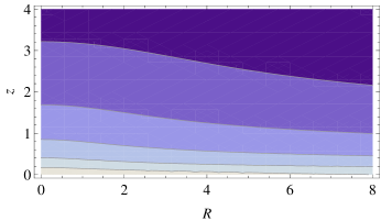
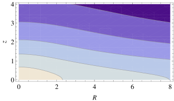
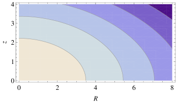
Figure 1: Logarithmic density contours in ($R,z$) plane for the missing model (11) with $b/a=0.1,1$ and 10. All the models are flattened, with $b/a\rightarrow 0$ being the razor-thin (Mestel) disc limit.

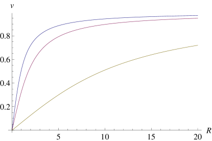
Figure 2: Rotation curves in units with $v_{0}=1$ in the equatorial plane for the missing model (11) with $b/a=0.1,1$ and 10. As $b/a\rightarrow 0$, the rotation curve attains its asymptotic value more quickly.

GENEALOGY

$${\displaystyle{GM\over r}}$$

Newtonian potential Isothermal models

Plummer (1911) model Cored Isothermal models

Hernquist (1990) model Evans & Williams (2014)

Kuzmin (1956) model Mestel (1963) model

Miyamoto Nagai (1975) model This paper

Table 1: The genealogy of models; the models in the right column are derived from the ones in the left by integration with respect to the model parameter $a$, together with the identification $v_{0}^{2}=GM/a$. The Plummer (1911) model sires the family of cored isothermal potentials (Wilkinson & Evans, 1999). In the limit $a\rightarrow 0$, the reduces to the Newtonian potential siring the singular isothermal sphere. The Hernquist (1990) model generates the cusped halo family recently discussed by Evans & Williams (2014). Likewise, the Kuzmin (1956) disc yields the family of cored Mestel discs (Evans & Collett 1993), which become Mestel’s (1963) model as $a\rightarrow 0$. Finally, the Miyamoto & Nagai (1975) disc sires the flat rotation curve models discussed in this paper.

2 Extremely Flat Halo Models

2.1 A Little History

Miyamoto & Nagai (1975) and Nagai & Miyamoto (1976) devised an ingenious way to build simple models of flattened galaxies. The models have become widely used. There are two reasons for this. First, the potential, and even more importantly, the force components are derived from simple, analytic functions. So they can speed N-body simulations with economy of effort. Second, the models may become arbitrarily flattened and so can represent the gamut of shapes of galaxies from spherical to disc-like.

Miyamoto & Nagai’s (1975) starting point was the desire to thicken up the infinitesimally thin Toomre (1963) discs. This family of discs has density

$$\rho_{\rm T}(R,z)=\Sigma(R)\delta(z)={\Sigma_{0}a^{2n+1}\over(R^{2}+a^{2})^{n+{\frac{1}{2}}}}\delta(z),\qquad n>0.$$ (1)

When $n$ is an integer greater than zero, Toomre (1963) showed that the corresponding potential is analytic. The simplest of the Toomre discs, corresponding to $n=1$, was previously discovered by Kuzmin (1956) and has the potential.

$$\psi_{\rm T}(R,z)={GM\over(R^{2}+(a+|z|)^{2})^{\frac{1}{2}}}.$$ (2)

The potentials of the higher Toomre discs can all be derived from the Kuzmin disc by differentiation with respect to the parameter $a^{2}$ (see e.g. Binney & Tremaine, 2008).

Miyamoto & Nagai (1975) hit upon the idea of making the replacement

$$|z|\rightarrow\sqrt{b^{2}+z^{2}}\doteq Z$$ (3)

in the potential of the Toomre discs. This indeed thickens them up and makes them versatile models of flattened galaxies. In particular, the Kuzmin disc (2), under the transformation (3), becomes exactly the simplest and most widely-used Miyamoto & Nagai (1975) model. In cylindrical polar coordinates ($R,\phi,z$), it has a gravitational potential

$$\psi_{1}(R,z)={GM\over(R^{2}+(a+Z)^{2})^{1/2}},\qquad\qquad Z^{2}=b^{2}+z^{2},$$ (4)

where $M$ is the mass of the galaxy, and $a$ and $b$ are two scalelengths. Using Poisson’s equation, the density corresponding to the potential (4)

$$\rho_{1}(R,z)={b^{2}M\over 4\pi}{aR^{2}+(a+3Z)(a+Z)^{2}\over Z^{3}(R^{2}+(a+Z)^{2})^{5/2}}.$$ (5)

Asymptotically, the density falls off like $\rho\sim R^{-3}$ (except if $a=0$) along the equatorial plane and like $\rho\sim z^{-5}$ along the pole. When $a=0$, the potential reduces to that of a spherical Plummer (1911) model. When $b=0$, the potential is that of a razor-thin Kuzmin (1956) disc. The potential (4) therefore provides an entire family of models which vary continuously between the Plummer sphere and the infinitesimally thin Kuzmin disc.

Just as the $n$th Toomre (1963) disc can be generated by differentiation $n$ times with respect to $a^{2}$, so Nagai & Miyamoto (1976) demonstrated that there is an entire family of thick disc models that can be generated from (5) by the same procedure. The family members satisfy the recurrence relations (Nagai & Miyamoto, 1976)

$$\psi_{n+1}(R,z) = \psi_{n}-{a\over 2n-1}{\partial\over\partial a}\psi_{n},$$ (6)

$$\rho_{n+1}(R,z) = \rho_{n}-{a\over 2n-1}{\partial\over\partial a}\rho_{n}.$$ (7)

They are known collectively as the Miyamoto & Nagai models (see e.g. Binney & Tremaine, 2008). The $n$th member of the family has density falling off like $R^{-2n-1}$ in the equatorial plane.

We shall now show that there is a model that has been missing all these years. It is the topmost model of the Miyamoto & Nagai family, corresponding to $n=0$, and it has a flat rotation curve.

2.2 The Missing Model

Evans & de Zeeuw (1992) discovered a simple potential-density pair for a disc with an asymptotically flat rotation curve

$$\Sigma(R)={\Sigma_{0}a\over\sqrt{a^{2}+R^{2}}},\qquad\psi(R,z)=-v_{0}^{2}\log\left[a+|z|+\sqrt{(a+|z|)^{2}+R^{2}}\right],$$ (8)

where $v_{0}^{2}=2\pi G\Sigma_{0}a$ (see also Evans & Collett, 1993). In the limit $a\rightarrow 0$ while maintaining $v_{0}$ fixed, the Mestel (1963) scale–free disc

$$\Sigma(R)={\Sigma_{0}a\over R},\qquad\psi(R)=-v_{0}^{2}\log(R),$$ (9)

is recovered. As Evans & de Zeeuw (1992) pointed out, the model (8) can be considered as a missing Toomre disc. It is really the $n=0$ member of the family (1). No doubt because it has the defect of infinite mass, it was not considered as an interesting model in the era before the discovery of flat rotation curves.

Proceeding analogously to Miyamoto & Nagai (1975), we thicken up the missing Toomre disc and arrive at the potential

$$\psi_{0}(R,z)=-v_{0}^{2}\log\left[a+Z+\sqrt{(a+Z)^{2}+R^{2}}\right],\qquad Z^{2}=b^{2}+z^{2}.$$ (10)

Application of Poisson’s equation gives the three dimensional density as

$$\rho_{0}(R,z)={v_{0}^{2}b^{2}\over 4\pi G}{R^{2}+(a+2Z)(a+Z)\over Z^{3}(R^{2}+(a+Z)^{2})^{\frac{3}{2}}}.$$ (11)

Here, $b>0$ without loss of generality. Then, the density is everywhere positive definite provided $a+b>0$. It is this model that we shall study in the remainder of the paper. It is the missing Miyamoto & Nagai model.

To substantiate our claim that this model should truly be considered part of the Miyamoto & Nagai (1975) family, we need only recall that each succeeding member of the sequence is generated by differentiation with respect to the scalelength $a$. So, if our model is indeed a missing relative, we expect it to satisfy the recurrence relations  (6) and  (7) with $n=0$. It can be easily verified that on setting $v_{0}^{2}=GM/a$ such is indeed the case.

Table 1 summarises the genealogy of some of the models discusses in this Section. The device of integration or differentiation with respect to the scalelength $a$ is simple, but surprisingly powerful. All the known flat rotation curve models can be derived from simple variants of the point mass potential (such as Plummer or Kuzmin) by this means.

Finally, we note that Zotos (2011) has introduced a related model described as “a combination of the logarithmic potential and a Miyamoto-Nagai model”. It has potential

$$\psi(R,z)=-{v_{0}^{2}\over 2}\log\left[(a+Z)^{2}+R^{2}\right],\qquad Z^{2}=b^{2}+z^{2}.$$ (12)

In the limit $b\rightarrow 0$, this does not correspond to a solution of Laplace’s equation everywhere except $z=0$, so it does not become an infinitesimally thin disc. Therefore, the model has properties that are rather different from the sequences studied by Miyamoto & Nagai (1975) and Nagai & Miyamoto (1976).

3 Model Properties

Here, we describe the properties of the potential-density pair give in eqns (10) and (11). Henceforth, to reduce notational clutter, we drop the subscript zero, which was introduced to establish that our models are the zeroth member of the Miyamoto & Nagai (1975) family.

3.1 Density

The density (11) falls off asymptotically like $\rho\sim R^{-1}$ in the equatorial plane, and like $\rho\sim z^{-4}$ along the pole. The models are always highly flattened. The limit $b\rightarrow 0$ gives an infinitesimally thin disc, which becomes the Mestel disc when additionally $a\rightarrow 0$.

More generally, Taylor expanding (11) about the origin tells us that the density there looks like

$$\rho(R,z)=\rho_{0}\Biggl{[}1-{R^{2}\over a_{1}^{2}}-{z^{2}\over a_{2}^{2}}-\cdots\Biggr{]},$$ (13)

with the axis ratio

$$\left({a_{2}\over a_{1}}\right)_{0}^{2}={b^{2}(a+4b)\over(a+b)(3a^{2}+9ab+8b^{2})}.$$ (14)

The model with $a=a_{\rm crit}=-\frac{1}{3}(19^{1\over 3}-4)=-.44387$ has spherical equidensity contours at the centre. If $a>a_{\rm crit}$, the models are oblate. If $-b<a<a_{\rm crit}$, the models are prolate at the centre. Irrespective of the behavior at the centre, the models all become extremely flattened and highly oblate, with an axis ratio $a_{2}/a_{1}\rightarrow 0$ at large radii. In other words, this family can exhibit a variety of behaviour near the centre, but is always disc-like at large radii.

Contours of constant density for some of the models are shown in Fig. 1. Note that they exhibit a range of behaviour including extreme flattenings. For modelling of galaxies, we remark that this represents the density contours of both the luminous and dark components, as the model already has a flat rotation curve. It is therefore straightforward to carve out a luminous exponential disc if we wish to separately identify and study the individual components.

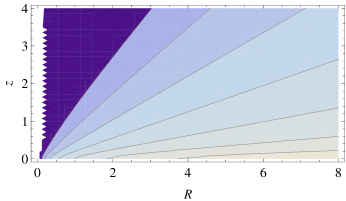
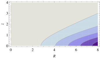
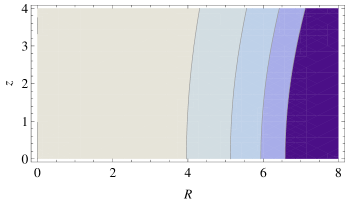
Figure 3: Contours of anisotropy parameter $\beta$ in ($R,z$) plane for the model (11) with $b/a=0.1,1$ and 10. With increasing flattening, the models become strongly tangentially anisotropic. In the uppermost panel, contours run from -0.1 to -1000, the anisotropy parameter increasing by a factor of 10 from one contour to the next. The model is dominate by extreme tangential anisotropy. In the middle panel, contours run from 0 to -10 in steps of -2, so the tangential anisotropy is significant but not overwhelming. In the lower panel, contours run from 0 to -0.08 in steps of -0,02, so the model is still nearly isotropic.

3.2 Kinematics

The force components are

$$F_{R} = -{Rv_{0}^{2}\over\sqrt{R^{2}+(a+Z)^{2}}(a+Z+\sqrt{R^{2}+(a+Z)^{2}})},$$

$$F_{z} = -{zv_{0}^{2}\over Z\sqrt{R^{2}+(a+Z)^{2}}}.$$ (15)

The rotation curve in the equatorial plane is

$$v_{\rm circ}^{2}(R)=v_{0}^{2}\left[1-{A\over\sqrt{R^{2}+A^{2}}}\right],\qquad A=a+b.$$ (16)

All the models have asymptotically flat rotation curves $v_{\rm circ}\rightarrow v_{0}$. Just as for the Miyamoto & Nagai models, the rotation curves are identical for all models with the same $A=a+b$. In particular, if $a+b=0$, the rotation curve is everywhere constant and equal to $v_{0}$. Some sample rotation curves are illustrated in Fig. 2.

By Jeans theorem (see e.g., Binney & Tremaine, 2008), the distribution function $F$ can only depend on the integrals of motion. For this axisymmetric potential, the two classical integrals are the binding energy and the angular momentum per unit mass. The velocity second moments for the two-integral $F(E,L_{z})$ can be found analytically, either by solving the Jeans equations or by using the Hunter (1977) formulae, which are

$$\rho\langle v_{R}^{2}\rangle = \rho\langle v_{z}^{2}\rangle=\int_{-\infty}^{\psi}\rho(\psi^{\prime},R^{2})d\psi^{\prime},$$ (17)

$$\rho\langle v_{\phi}^{2}\rangle = \int_{-\infty}^{\psi}{\partial\over\partial R}\bigl{(}R\rho(\psi^{\prime},R^{2})\bigr{)}d\psi^{\prime},$$ (18)

Here, the density has been written as an explicit function of $R$ and $\psi$, rather than $R$ and $z$. This can be done, as

$$Z(z)={\frac{1}{2}}\left(\exp(-\psi/v_{0}^{2})-R^{2}\exp(\psi/v_{0}^{2})\right)-a,$$ (19)

Substituting into (11) gives $\rho(\psi,R^{2})$. The integrations in Hunter’s formulae can be explicitly performed to give an analytic solution of the Jeans equations as

$$\langle v_{R}^{2}\rangle=\langle v_{z}^{2}\rangle={v_{0}^{2}\over 2}\,{Z\sqrt{R^{2}+(a+Z)^{2}}\over R^{2}+(a+Z)(a+2Z)}$$ (20)

$$\langle v_{\phi}^{2}\rangle={v_{0}^{2}\over 2}\,{2R^{2}+2(a+Z)(a+2Z)-(2a+3Z)\sqrt{R^{2}+(a+Z)^{2}}\over R^{2}+(a+Z)(a+2Z)}$$ (21)

The velocity second moment tensor is aligned in cylindrical polar coordinates so the cross-terms vanish, i.e., $\langle v_{R}v_{z}\rangle=0=\langle v_{R}v_{\phi}\rangle=\langle v_{z}v_{\phi}\rangle$. The models are isotropic on the pole $R=0$, but everywhere else, $\langle v_{\phi}^{2}\rangle>\langle v_{R}^{2}\rangle$. In the equatorial plane as $r\rightarrow\infty$, $\langle v_{R}^{2}\rangle\rightarrow 0$ whilst $\langle v_{\phi}^{2}\rangle\rightarrow v_{0}^{2}$. Contours of the second moment anisotropy parameter

$$\beta=1-{\langle v_{\phi}^{2}\rangle\over\langle v_{R}^{2}\rangle}$$ (22)

are shown in Fig. 3. In the equatorial plane, as $R\rightarrow\infty$, $\beta\rightarrow-2R/b$ and so the model becomes increasingly dominated by circular orbits.

So far, the models have no stellar rotation. The maximum streaming model is created by reversing all stars with $L_{z}<0$, so that all stars rotate in the same direction. The maximum mean streaming velocity at any point ($R,z$) is

$$\langle v_{\phi}\rangle={\sqrt{2}\over\pi\rho}\int_{-\infty}^{\psi}{d\psi^{\prime}\over\sqrt{\psi-\psi^{\prime}}}\int_{0}^{R}{dR^{\prime}\over\sqrt{R^{2}-R^{\prime 2}}}{\partial\over\partial R}R\rho(\psi^{\prime},R^{\prime 2})$$ (23)

This is easily evaluated numerically – Fig. 4 shows the maximum streaming velocity for the model with $b/a=1$.

To summarise, the second moments of the model are all analytic, whilst the maximum mean streaming velocity is a simple quadrature. This enables models to be built with a wide range of kinematic properties.

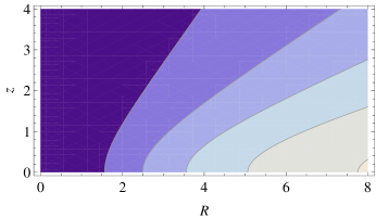
Figure 4: Contours of maximum mean streaming velocity in ($R,z$) plane for the model (11) with $b/a=1$. Contours run from 0.4 to 0.8 in units with $v_{0}=1$.

Figure 5: Plots of the even part of the distribution function for the model (11) with $b/a=1$. Upper panel: the DF in integral space ($E,L_{z}$). Lower panel: the velocity distribution ($v_{\phi},v_{\rm T}$) in the equatorial plane at $(R,z)=(2a,0)$. Here, $v_{\rm T}=\sqrt{v_{R}^{2}+v_{z}^{2}}$.

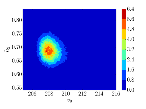
Figure 6: The model (11) is fitted to the rotation curve data of Sofue et al. (2009) and the vertical velocity dispersion data of populations of thick disc stars given in Smith et al. (2012) and Moni Bidin et al. (2012). The plots show likelihood contours in the plane of the recovered model parameters $v_{0}$, $a$ and $b$, together with the scale heights of the two populations $h_{1}$ and $h_{2}$. The colour scheme shows the normalized posterior probability density. The posterior values for the model parameters are $v_{0}=208.3^{+0.7}_{-1.2}$ kms^-1, $a=-2.53^{+0.20}_{-0.18}$ and $b=2.58^{+0.17}_{-0.20}$, whilst the scaleheights are $h_{1}=426^{+12}_{-14}$ pc and $h_{2}=689^{+31}_{-37}$ pc respectively.

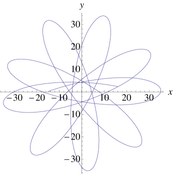
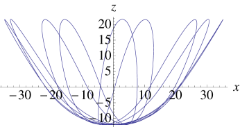
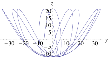
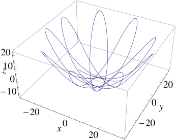
Figure 7: Plots showing the orbit of the Sgr for the best fit model parameters in the three principal planes. The orbit has a pericentric distance of 0.6 kpc, apocentre of 60.2 kpc and a maximum height above the disc of 30.8 kpc. The integration time is $\sim 5$ Gyr. The trajectory is recognized as a precessing banana orbit.

3.3 The Distribution Function

For some applications – such as studies of the stability of highly flattened galaxies  (Merritt & Sellwood, 1994) – it is useful to have the full distribution function (DF) of the model. For our application, we do not need the precise form of the DF, but we do need to be certain that the models are physical and correspond to an everywhere positive DF. This is not a matter of idle pettifoggery ! The well-known flattened logarithmic model fails to be physical once its equipotential axis ratio is less than $1/\sqrt{2}\approx 0.707$, and so cannot attain very extreme ellipticities (Evans, 1993; Binney & Tremaine, 2008). Without constructing the DF and checking it is positive, we cannot be sure that our potential-density pair really do correspond to viable halo models.

For our models, the density $\rho(\psi,R^{2})$ is

$$\rho(\psi,R^{2}) = {4b^{2}v_{0}^{2}\over\pi G}\Biggl{[}{\exp{4\psi}\over(1+R^{2}\exp(2\psi))(1-2a\exp(\psi)-R^{2}\exp(2\psi))^{3}}\Biggr{.}$$ (24)

$$+ \Biggl{.}{\exp{4\psi}\over(1+R^{2}\exp(2\psi))^{3}(1-2a\exp(\psi)-R^{2}\exp(2\psi))^{2}}\Biggr{]}$$

The even part of the two-integral DF is given by Hunter & Qian (1993) as the contour integral

$${F_{\rm even}}(E,L_{z}^{2})={1\over 4\pi^{2}i\sqrt{2}}{\partial^{2}\over\partial E^{2}}\int_{-\infty}^{E+}{d\psi\over(\psi-E)^{1/2}}\rho\Biggl{(}\psi,{L_{z}^{2}\over 2(\psi-E)}\Biggr{)}.$$ (25)

A cut is needed in the complex plane from $\psi=E$ to $\psi=-\infty$ to define the square root function. The contour is a loop that starts on the lower side of the real $\psi$ axis at $\psi=-\infty$. The circle encircles $\psi=E$ in the positive sense, crossing the real axis at $\psi={\psi_{\rm env}}(E)$ and ending at $\psi=-\infty$ on the upper side of the real axis. Here,

$${\psi_{\rm env}}(E)=\psi({R_{\rm c}}(E),0)$$ (26)

where ${R_{\rm c}}$ is the radius of the circular orbit in the equatorial plane with energy $E$. The circular orbits are defined parametrically by

$$E = -v_{0}^{2}\log(A+\sqrt{{R_{\rm c}}^{2}+A^{2}})-{L_{z}^{2}\over 2{R_{\rm c}}^{2}}$$

$$L_{z}^{2} = {{R_{\rm c}}^{4}v_{0}^{2}\over\sqrt{{R_{\rm c}}^{2}+A^{2}}(A+\sqrt{{R_{\rm c}}^{2}+A^{2}})}$$ (27)

So, $\psi_{\rm env}$ is the root of the equation

$$2({\psi_{\rm env}}-E)-v_{0}^{2}+{Av_{0}^{2}\over\exp(-{\psi_{\rm env}}/v_{0}^{2})-A}=0$$ (28)

As the density in eq. (24) is a rational function, there are no further branch cuts needed and so it is straightforward to devise a contour. For ease of numerical evaluation, it must not come too close to the cut along the real axis. For our calculations, we choose to parametrize the bottom half of the contour by

$$\psi=y+\psi_{\rm env}(E)+i\epsilon(\exp(y)-1),\qquad\qquad-\infty\leq y\leq 0,$$ (29)

where $\epsilon$ is small. We then obtain the distribution function by doubling the real part along it.

The DF is shown in Fig. 5 both in the space of integrals ($E,L_{z}$) and in velocities ($v_{\phi},v_{\rm T}$), where $v_{\rm T}=\sqrt{v_{R}^{2}+v_{z}^{2}}$). The flattening of the model at large radii is produced by the bias towards circular orbits, as indicated by the rise of the DF towards the edge of the domain in the upper panel. As this is an even DF, there are equal numbers of rotating and counter-rotating stars, and these show up as two peaks in the velocity distributions in the lower two panels corresponding to near-circular orbits. It is of course straightforward to produce discs of stars rotating in one direction, for example, by doubling the part of the DF corresponding to positive $v_{\phi}$ and nulling the part corresponding to negative $v_{\phi}$.

Evaluations on a numerical grid confirm that the even DF is everywhere positive. This guarantees that the underlying model is physical, even for very severely flattened configurations.

4 Application: The Flattening of the Galaxy

4.1 Data

Two independent constraints on the potential of the Galaxy are the rotation of the HI gas in the Galactic plane and the kinematics of stars perpendicular to the plane. These data have been examined many times before. Most previous investigations have used a model that is decomposed into disc and spherical halo with the aim of constraining the local dark matter density. Here, our focus is different. We will not make any distinction between baryonic and dark matter and seek to put constraints on the overall flattening of the potential and density of the Galaxy.

The study of the kinematics of vertical tracers of stars near the Sun goes back to the very origins of the dark matter problem (Oort, 1932). The underlying idea is to use a volume complete survey of stars with known distances and kinematics to constrain the gravitational potential either with distribution functions or with the Jeans equations (see e.g., Kuijken & Gilmore, 1989a, b; Holmberg & Flynn, 2004; Smith et al., 2012). Often, the potential is parametrised in a simple way, encoding prior beliefs as to the likely density of disc and halo. So, for example, Kuijken & Gilmore (1989b) use a simple potential mimicking the effects of disc and halo, together with a prior on the rotation curve.

By itself, the rotation curve of the Milky Way provides no constraint on the flattening of the density, as models that are spherical, spheroidal or disc-like can all possess flat rotation curves. From the perspective of the local dark matter density, this has been recently emphasized by Weber & de Boer (2010). They use a variety of spherical and spheroidal halo models coupled with baryonic thin and thick exponential discs to reproduce the rotation curve and find the local dark matter density is uncertain by at least a factor of 2. Here, we make no attempt at a decomposition into disc and halo components, but model the entire potential and density of the Galaxy by eqs (10) and (11). Our aim is to understand how flattened the density contours of the Galaxy could possibly be, given the constraints from the vertical kinematics of stars in the solar neighbourhood and the behaviour of the rotation curve from 4kpc to 20 kpc.

We use the data on the vertical kinematics from two sources. First, Smith et al. (2012) use samples of dwarf stars extracted from the Sloan Digital Sky Survey Stripe 82 catalogue (Bramich et al. 2008). They provide the vertical and radial velocity dispersions as a function of $z$ up to 2.5 kpc below the Galactic plane. Second, Moni Bidin et al. (2012) provide the variation of velocity dispersion with $z$ using the velocities of $\sim 400$ red giants towards the South Galactic Pole. These thick disc stars extend to heights of up to 4.5 kpc from the Galactic plane.

Complementing this, we also require that the models match the rotation curve of the Galaxy. For the inner Galaxy, this is determined by the terminal velocities of HI and CO gas , for the outer Galaxy from spectrophotometry of HII and CO regions  (e.g., Fich et al., 1989). The variety of methods does lead to some scatter, but Sofue et al. (2009) has recently compiled and re-analysed the data, calibrating it to Galactic constants of Solar position of 8 kpc and Local Standard of Rest of 200 kms^-1.

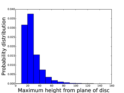
Figure 8: Histogram showing the maximum distance from the plane of the disc reached by $10^{4}$ Sgr orbits, integrated backwards with starting condition drawn from the current error circle on position and velocity. Only 4.3 % of the orbits reach a height greater than 50 kpc, and 2.25 % a height greater than 60 kpc.

4.2 Results

Given the model parameters $v_{0},a,b$, the rotation curve in the Galactic plane ($z=0$) is given by eqn (16). We can also calculate the vertical velocity dispersion for a tracer population as a function of $z$ at the radius $R=R_{\odot}$ via direct integration of the vertical Jeans equation, assuming the vertical density distribution of the tracers is known. We have two sources of data for the vertical velocity dispersion (Smith et al., 2012; Moni Bidin et al., 2012) and we assume these data are well represented by two distinct exponential density distributions with scale heights $h_{1}$ and $h_{2}$. This is a common assumption, supported by the original work identifying the Galactic thick disc  (Gilmore & Reid, 1983), as well as photometry of external thick discs in edge-on galaxies, which show exponentially declining profiles at large heights (Yoachim & Dalcanton, 2006). Nonetheless, hard evidence that the density law of thick disc populations in our Galaxy declines exponentially at these heights is actually rather elusive.

Together with the 3 model parameters, the two disc scale-heights provide a 5-dimensional parameter space. The calculated values of the rotation curve and vertical velocity dispersion can then be compared to our data, with the likelihood value for these parameters given by $\exp(-\chi^{2})$.

In order to explore this parameter space, we use the open source Monte Carlo Markov Chain code $emcee$ provided by Foreman-Mackey et al. (2013). Contour plots of the recovered potential and scale-height parameters are shown in Fig. 6. The posterior values for the model parameters, together with the $1\sigma$ bounds, are $v_{0}=208.3^{+0.7}_{-1.2}$ kms^-1, $a=-2.53^{+0.20}_{-0.18}$, $b=2.58^{+0.17}_{-0.20}$. The scaleheights of the thick disc stars using the data of Smith et al. (2012) and Moni Bidin et al. (2012) are $h_{1}=426^{+12}_{-14}$ pc and $h_{2}=689^{+31}_{-37}$ pc respectively. The flatness of the rotation curve provides the constraints on $v_{0}$ and $a+b$, whilst the vertical velocity data constrains the population scale heights and the individual values of $a$ and $b$. Flatter density distributions than this can recover the rotation curve, but then they underpredict the run of vertical velocity dispersion at large heights ($\sim 4$ kpc) from the Galactic plane. In our best fit model, the axis ratio of the equidensity contour that passes through the Solar position is $0.57$. Models with more extreme flattening than this are ruled out.

To confirm our result that extreme flattenings are not possible, we can use the Sagittarius (Sgr) tidal stream. In a spherical potential, the debris from the Sgr stream would be confined to a plane. In a nearly-spherical potential, the plane slowly precesses. When the gravitational field is highly flattened, then there are two problems. First, the potential may generate more precession than is actually observed. This idea was first proposed by Johnston et al. (2005), who measured a difference between the mean orbital poles of the leading and trailing debris of $10.4\pm 2.6^{\circ}$ as delineated by M giants from the Two Micron All-Sky Survey. The much richer and higher quality Sloan Digital Sky Survey data has recently been re-analysed by Belokurov et al. (2014), who found a more complex pattern of differential precession in the bright and faint Sgr streams. For our purposes here, we summarise Figure 13 of Belokurov et al. (2014) by the statement that the magnitude of the precession of the wraps of the leading and trailing debris is certainly less than $15^{\circ}$. Secondly, the present day kinetic energy of the Sgr dwarf is known to reasonable accuracy, as its proper motion has been measured (Dinescu et al., 2005). If the equipotentials are highly flattened, then the Sgr cannot rise high enough above the Galactic plane to provide the debris in the tails. We note that Sgr stream stars have been detected at heights of $\sim 60$ kpc above the Galactic plane by (see e.g., Majewski et al., 2003; Belokurov et al., 2014). This is a serious challenge if the halo flattening is substantial.

Using our best fit model parameters, we integrate the orbit of the Sagittarius dwarf Galaxy backwards from its present day position of $[x,y,z,v_{x},v_{y},v_{z}]=[-16.1,2.4,-6.1,232,-47,190]$ in units of kpc and kms^-1 (see e.g., Gibbons et al., 2014). The results of this integration are shown in Fig. 7, which show the Sgr moving on a precessing banana orbit. This is a typical orbit for starting positions within the observational errors. There are two immediate and related problems. First, the view of the orbit in the ($x,y$) plane makes it clear that the precession angle is too great. From one apocentre to the next, the orbital plane turns through $\sim 43^{\circ}$, which is too large to be consistent with the data. Second, the maximum height of the orbit above the Galactic plane is just $\sim 31$ kpc. In flattened potentials, the Sgr does not have enough kinetic energy to reach high enough above the Galactic plane to generate all the known debris. To emphasise this point, we show in Fig. 8 a histogram of the maximum heights above the disc for a range of potential parameters from our posterior distribution, drawing Sgr co-ordinates from within the current observational errors. We find that just 2.25 % of all the orbits reach a height of greater than $\sim 60$ kpc. With increasing accuracy of the proper motions, this result could probably be tightened further. Before then, improved modelling without the assumption that a stream is an orbit is really needed (e.g., Gibbons et al. 2014). We plan to return to this problem in a later publication.

Throughout, we have modelled the entire Galactic potential, making no distinction between the disc and halo components. It follows that our constraint that $q\gtrsim 0.57$ applies to the equidensity contours of the total matter distribution. However, the luminous thin and thick discs of the Galaxy are known to be highly flattened. For example, the scalelengths of the thin and thick discs are $2.8\pm 0.3$ kpc and $3.7\pm 0.5$ kpc respectively, whilst the scaleheights range between 350 pc to 1kpc  (Ojha, 2001). Rather than indulge in uncertain decompositions into disc and halo, we merely note that – if the overall flattening satisfies $q\gtrsim 0.57$ – then this must assuredly be true of the dark halo by itself. Indeed, the dark halo itself must be considerably rounder than our limiting value of E4 or $q=0.57$)!

5 Conclusions

We have introduced a new family of very highly flattened galaxy models. Although the density contours can be spherical, oblate or prolate in the central regions, the strongly disc-like nature of the models rapidly asserts itself at moderate to large radii. The circular velocity curve of all the models is asymptotically flat. They are the only flat rotation curve models known to us whose properties can represent three-dimensional thickened disks as well as haloes.

The family are related to a number of classical models already in the literature. In the infinitesimally thin limit, they become cored Mestel discs (Mestel, 1963; Evans & Collett, 1993). So, the family can be thought of as thickened, fully three-dimensional Mestel discs. They are also part of the Miyamoto & Nagai (1975,1976) sequence of flattened galaxy models, albeit missing from the original works which predated the discovery and widespread acceptance of flat rotation curves.

The kinematic properties of the model are largely analytic. In particular, the solutions of the Jeans equations in cylindrical polar coordinates are straightforward. The two integral distribution function $F(E,L_{z})$ has been derived as a quadrature. It is everywhere positive definite for arbitrarily severe flattenings. The highly flattened shape is supported by extreme values of the azimuthal velocity second moment $\langle v_{\phi}^{2}\rangle$, or in physical terms by tangential anisotropy or by rotation.

There has long been a lacuna of models with simple properties that are highly flattened. The logarithmic halo model, for example, ceases to be physical below a flattening in the equipotentials of $q=1/\sqrt{2}$ (Evans, 1993; Binney & Tremaine, 2008), thus preventing exploration of highly elongated shapes. So, our new models have a number of applications, for example in the study of the stability of highly flattened galaxies to bending modes (Merritt & Sellwood, 1994) and instabilities of thickened discs with counter-rotating stars (Sellwood & Merritt, 1994). They also provide natural models of dark haloes for theories in which the dark matter is cold atomic or molecular gas (Pfenniger et al., 1994; Pfenniger & Combes, 1994; Davies, 2012) or is very highly flattened, as in the decaying neutrino hypothesis (Sciama, 1993). They can be used to assess the claims of highly flattened haloes in some nearby galaxies, such as NGC 4244 (Olling, 1996), NCC 891 (Becquaert & Combes, 1997) and NGC 4650 (Combes & Arnaboldi, 1996). Another application is to the dark discs that can form in $\Lambda$CDM as a consequence of satellite accretion (Read et al., 2008).

We have used the models to study the overall shape of the Galaxy. Here, the vertical kinematics of stars in the solar neighbourhood together with the rotation curve constrain the shape of the density contours to be rounder than $q\approx 0.6$. If the shape the Galaxy is more highly flattened than this, it is not possible to reproduce the gently rising run of velocity dispersion with height for stars above or below the Galactic plane. Confirmation of this is provided by the Sgr dwarf galaxy. The present-day phase space coordinates of the Sgr are known. Given this kinetic energy, then if the halo is flatter than $q\approx 0.6$, the orbit cannot reach $\sim 60$ kpc above the Galactic plane where Sgr debris is detected. Highly flattened potentials also generate too much orbital plane precession to be consistent with the debris.

Given that our constraint is on the overall equidensity contours, and the luminous baryonic material is already known to be highly flattened, this means that the shape of the dark matter halo alone at least for our Galaxy must be considerably rounder than E4 (or $q=0.57$). This therefore rules out theories in which the dark matter is highly flattened – in particular the suggestion that cold neutral or molecular gas in the disc can generate the flat rotation curve.

Of course, many papers have studied the flattening of the halo of the Milky Way, using techniques such as the stellar kinematics of halo stars (Smith et al., 2009; Loebman et al., 2012), cold stellar streams (Koposov et al., 2010) and the Sagittarius stream (Helmi, 2004; Fellhauer et al., 2006). Given the discrepancies between results, there are clearly substantial degeneracies and establishing the precise flattening will require careful fitting to multiple datasets. Nonetheless, some regions of parameter space can be robustly excluded and some definite results obtained. The virtue of the approach in this paper is that we have shown that extremely flattened halo models (ellipticity greater than 0.43) are inconsistent with both the stellar kinematics and the Sagittarius stream.

References

- Abadi et al. (2010) Abadi M. G., Navarro J. F., Fardal M., Babul A., Steinmetz M., 2010, MNRAS, 407, 435
- Allgood et al. (2006) Allgood B., Flores R. A., Primack J. R., Kravtsov A. V., Wechsler R. H., Faltenbacher A., Bullock J. S., 2006, MNRAS, 367, 1781
- Becquaert & Combes (1997) Becquaert J.-F., Combes F., 1997, AA, 325, 41
- Belokurov et al. (2014) Belokurov V., Koposov S. E., Evans N. W., Peñarrubia J., Irwin M. J., Smith M. C., Lewis G. F., Gieles M., Wilkinson M. I., Gilmore G., Olszewski E. W., Niederste-Ostholt M., 2014, MNRAS, 437, 116
- Binney & Tremaine (2008) Binney J., Tremaine S., 2008, Galactic Dynamics: Second Edition. Princeton University Press
- Combes & Arnaboldi (1996) Combes F., Arnaboldi M., 1996, AA, 305, 763
- Davies (2012) Davies J., 2012, ArXiv e-prints
- Deason et al. (2011) Deason A. J., McCarthy I. G., Font A. S., Evans N. W., Frenk C. S., Belokurov V., Libeskind N. I., Crain R. A., Theuns T., 2011, MNRAS, 415, 2607
- Deg & Widrow (2013) Deg N., Widrow L., 2013, MNRAS, 428, 912
- Dinescu et al. (2005) Dinescu D. I., Girard T. M., van Altena W. F., Lopez C., 2005, ApJL, 618, L25
- Evans (1993) Evans N. W., 1993, MNRAS, 260, 191
- Evans & Collett (1993) Evans N. W., Collett J. L., 1993, MNRAS, 264, 353
- Evans & de Zeeuw (1992) Evans N. W., de Zeeuw P. T., 1992, MNRAS, 257, 152
- Evans & Williams (2014) Evans N. W., Williams A., 2014, MNRAS, in press
- Fellhauer et al. (2006) Fellhauer M., Belokurov V., Evans N. W., Wilkinson M. I., Zucker D. B., Gilmore G., Irwin M. J., Bramich D. M., Vidrih S., Wyse R. F. G., Beers T. C., Brinkmann J., 2006, ApJ, 651, 167
- Fich et al. (1989) Fich M., Blitz L., Stark A. A., 1989, ApJ, 342, 272
- Foreman-Mackey et al. (2013) Foreman-Mackey D., Hogg D. W., Lang D., Goodman J., 2013, PASP, 125, 306
- Gibbons et al. (2014) Gibbons S., Belokurov V., Evans N. W., 2014, ArXiv e-prints
- Gilmore & Reid (1983) Gilmore G., Reid N., 1983, MNRAS, 202, 1025
- Helmi (2004) Helmi A., 2004, ApJL, 610, L97
- Hernquist (1990) Hernquist L., 1990, ApJ, 356, 359
- Holmberg & Flynn (2004) Holmberg J., Flynn C., 2004, MNRAS, 352, 440
- Hunter (1977) Hunter C., 1977, AJ, 82, 271
- Hunter & Qian (1993) Hunter C., Qian E., 1993, MNRAS, 262, 401
- Johnston et al. (2005) Johnston K. V., Law D. R., Majewski S. R., 2005, ApJ, 619, 800
- Knee & Brunt (2001) Knee L. B. G., Brunt C. M., 2001, Nature, 412, 308
- Koposov et al. (2010) Koposov S. E., Rix H.-W., Hogg D. W., 2010, ApJ, 712, 260
- Kuijken & Gilmore (1989a) Kuijken K., Gilmore G., 1989a, MNRAS, 239, 605
- Kuijken & Gilmore (1989b) Kuijken K., Gilmore G., 1989b, MNRAS, 239, 571
- Kuzmin (1956) Kuzmin G., 1956, Astron. Zh, 33, 27
- Law & Majewski (2010) Law D. R., Majewski S. R., 2010, ApJ, 714, 229
- Loebman et al. (2012) Loebman S. R., Ivezić Ž., Quinn T. R., Governato F., Brooks A. M., Christensen C. R., Jurić M., 2012, ApJL, 758, L23
- Majewski et al. (2003) Majewski S. R., Skrutskie M. F., Weinberg M. D., Ostheimer J. C., 2003, ApJ, 599, 1082
- Merritt & Sellwood (1994) Merritt D., Sellwood J. A., 1994, ApJ, 425, 551
- Mestel (1963) Mestel L., 1963, MNRAS, 126, 553
- Miyamoto & Nagai (1975) Miyamoto M., Nagai R., 1975, PASJ, 27, 533
- Moni Bidin et al. (2012) Moni Bidin C., Carraro G., Méndez R. A., 2012, ApJ, 747, 101
- Nagai & Miyamoto (1976) Nagai R., Miyamoto M., 1976, PASJ, 28, 1
- Ojha (2001) Ojha D. K., 2001, MNRAS, 322, 426
- Olling (1996) Olling R. P., 1996, AJ, 112, 481
- Oort (1932) Oort J. H., 1932, BAIN, 6, 249
- Pfenniger & Combes (1994) Pfenniger D., Combes F., 1994, AA, 285, 94
- Pfenniger et al. (1994) Pfenniger D., Combes F., Martinet L., 1994, AA, 285, 79
- Plummer (1911) Plummer H. C., 1911, MNRAS, 71, 460
- Read et al. (2008) Read J. I., Lake G., Agertz O., Debattista V. P., 2008, MNRAS, 389, 1041
- Sciama (1993) Sciama D. W., 1993, Modern cosmology and the dark matter problem. Cambridge University Press
- Sciama (1999) Sciama D. W., 1999, in Harvey A., ed., On Einstein’s Path: essays in honor of Engelbert Schucking Decaying Neutrinos and the Flattering of the Galactic Halo. p. 443
- Sellwood & Merritt (1994) Sellwood J. A., Merritt D., 1994, ApJ, 425, 530
- Smith et al. (2009) Smith M. C., Evans N. W., An J. H., 2009, ApJ, 698, 1110
- Smith et al. (2012) Smith M. C., Whiteoak S. H., Evans N. W., 2012, ApJ, 746, 181
- Sofue et al. (2009) Sofue Y., Honma M., Omodaka T., 2009, PASJ, 61, 227
- Sofue & Rubin (2001) Sofue Y., Rubin V., 2001, ARAA, 39, 137
- Toomre (1963) Toomre A., 1963, ApJ, 138, 385
- Weber & de Boer (2010) Weber M., de Boer W., 2010, AA, 509, A25
- Wilkinson & Evans (1999) Wilkinson M. I., Evans N. W., 1999, MNRAS, 310, 645
- Yoachim & Dalcanton (2006) Yoachim P., Dalcanton J. J., 2006, AJ, 131, 226
- Zemp et al. (2012) Zemp M., Gnedin O. Y., Gnedin N. Y., Kravtsov A. V., 2012, ApJ, 748, 54
- Zotos (2011) Zotos E. E., 2011, New Ast, 16, 391